Figure 1.
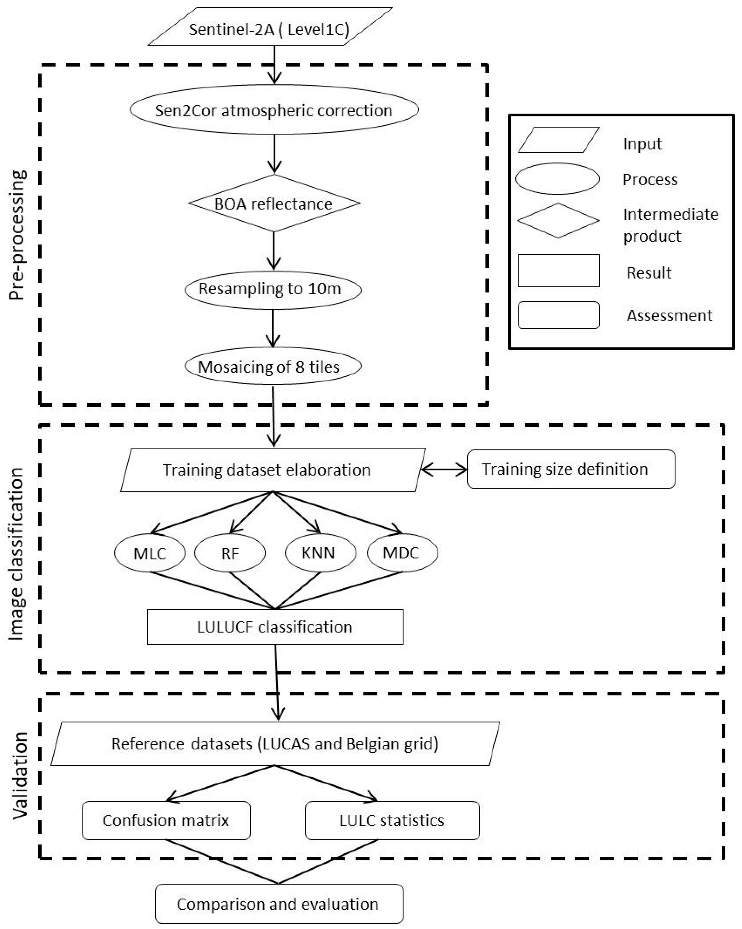
Workflow of the Land Use, Land Use Change, and Forestry (LULUCF) classifications with Sentinel-2 imagery.
Figure 1.
Workflow of the Land Use, Land Use Change, and Forestry (LULUCF) classifications with Sentinel-2 imagery.
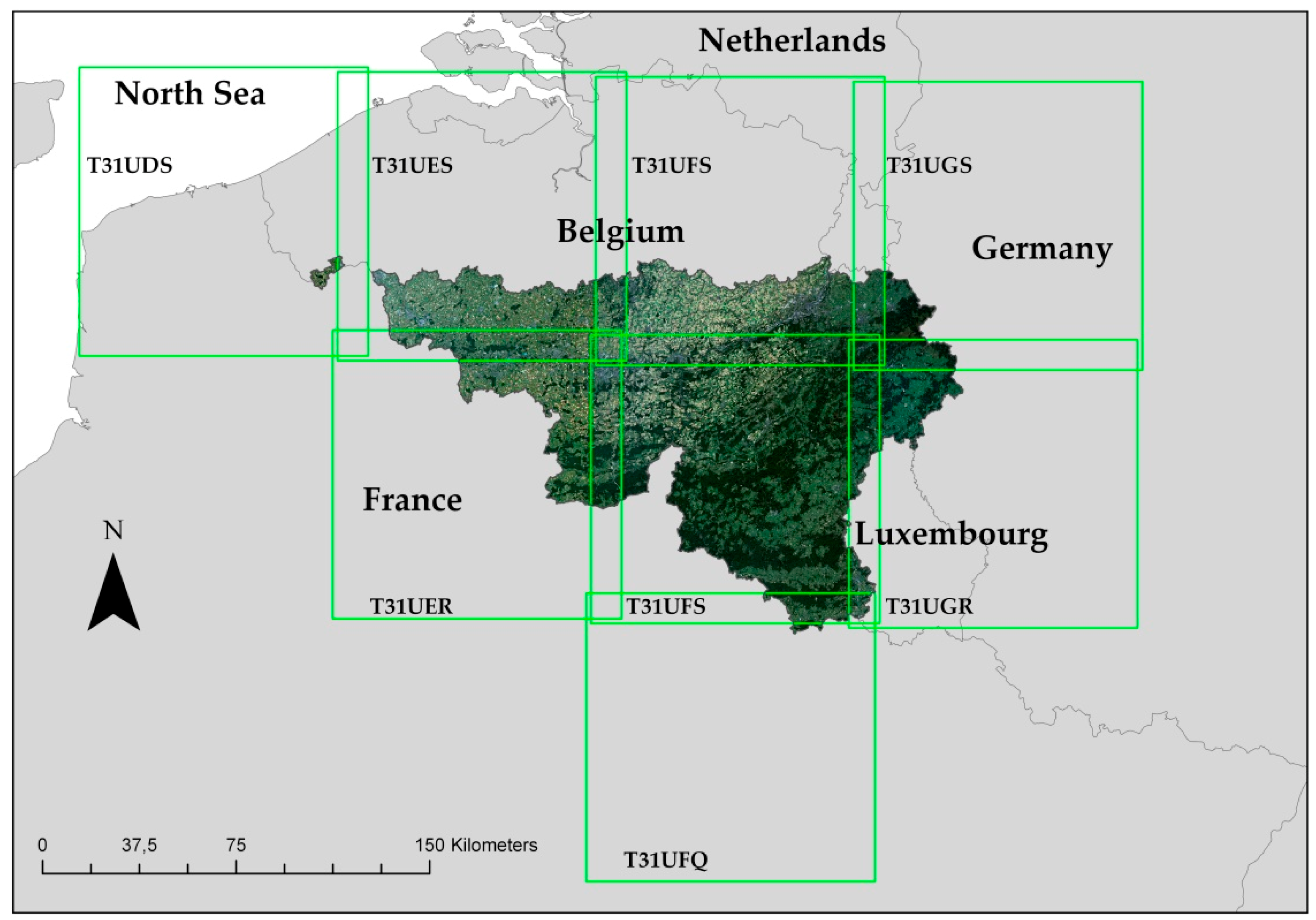
Figure 2.
Tiles arrangement allowing the realization of the three mosaics of Sentinel-2 in Wallonia, Belgium. Eight tiles (T31UDS, T31UES, T31UFS, T31UGS, T31UER, T31UFS, T31UGR, and T31UFQ) were used to produce three mosaics. The data spanned from December 2016 (winter mosaic), March to May 2016 (spring mosaic), and July to September 2016 (summer mosaic). The mosaics were cloud-free and characterized by a uniform leaf-on state of the trees.
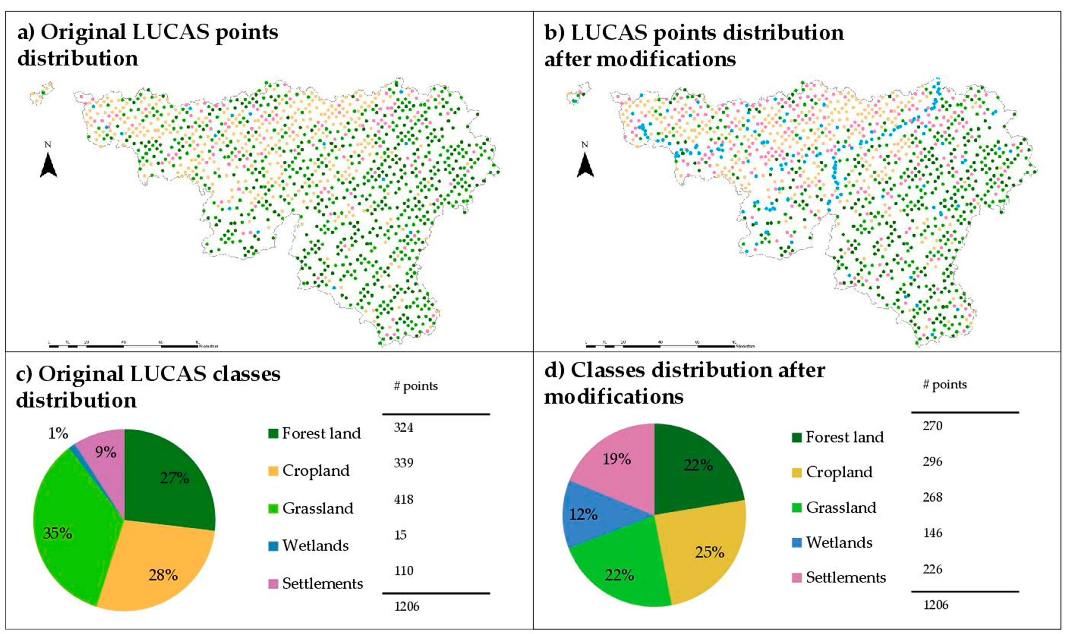
Figure 3.
Distribution of the training data in Wallonia, Belgium. (a) The original Land Use/Cover Area frame statistical Survey (LUCAS) points were composed of 1206 points distributed all around Wallonia (forest land = 324 points; cropland = 339 points; grassland = 418 points; wetlands = 15 points; settlements = 110 points). To avoid a class imbalance problem, the location of some points was modified. (b) After the modification, the distribution of the points was: forest land = 270 points; cropland = 296 points; grassland = 268 points; wetlands = 146 points; settlements = 226 points. (c,d) show a pie chart of the classes distribution for the original and modified LUCAS points.
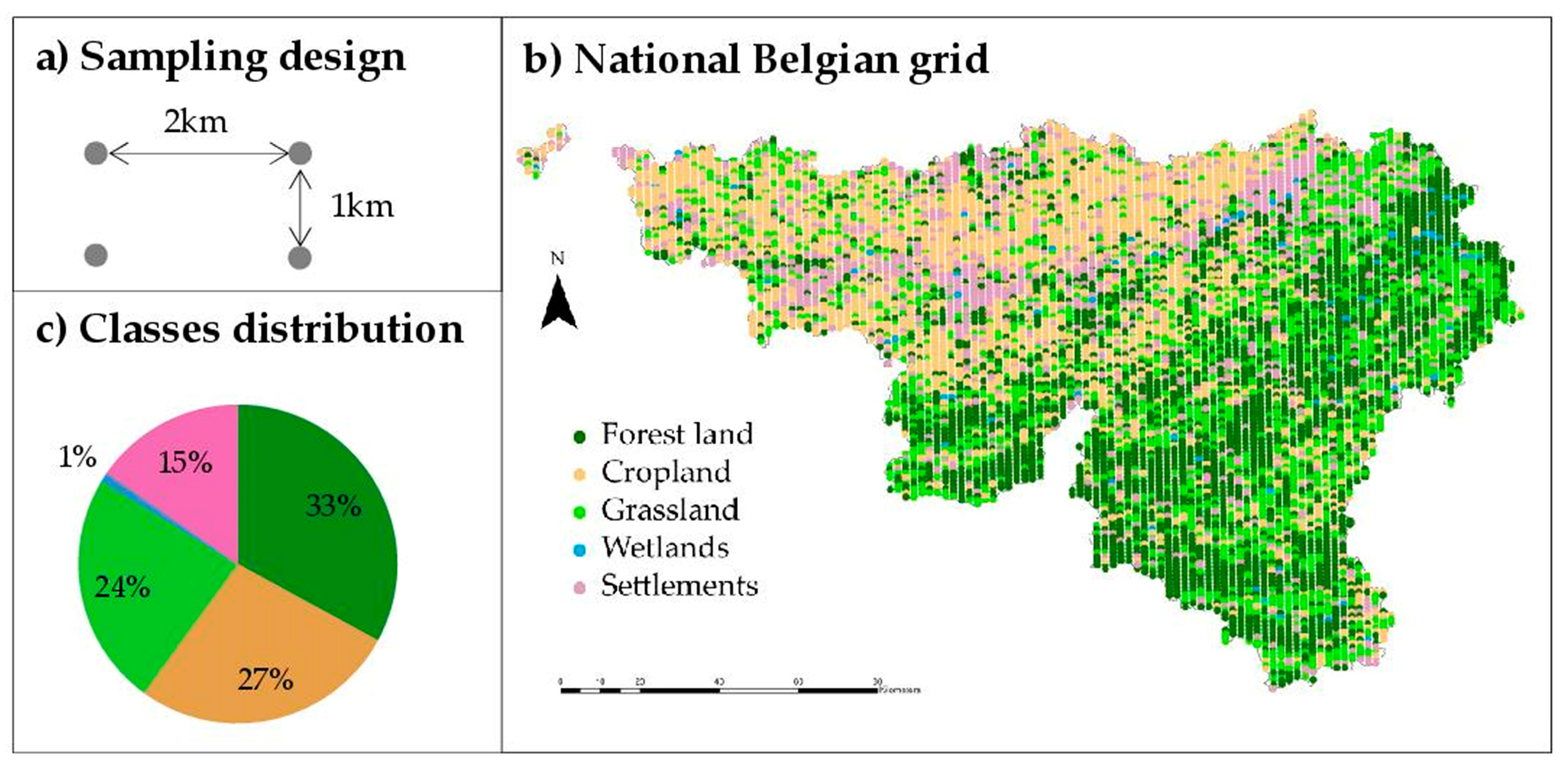
Figure 4.
Distribution of the national Belgian grid in Wallonia, Belgium. (a) Explanation of the sampling design; (b) Distribution of the points. It is composed of 8439 points distributed all around Wallonia (forest land = 2782 points; cropland = 2282 points; grassland = 2002 points; wetlands = 80 points; settlements = 1293 points); (c) Pie chart of the classes distribution.
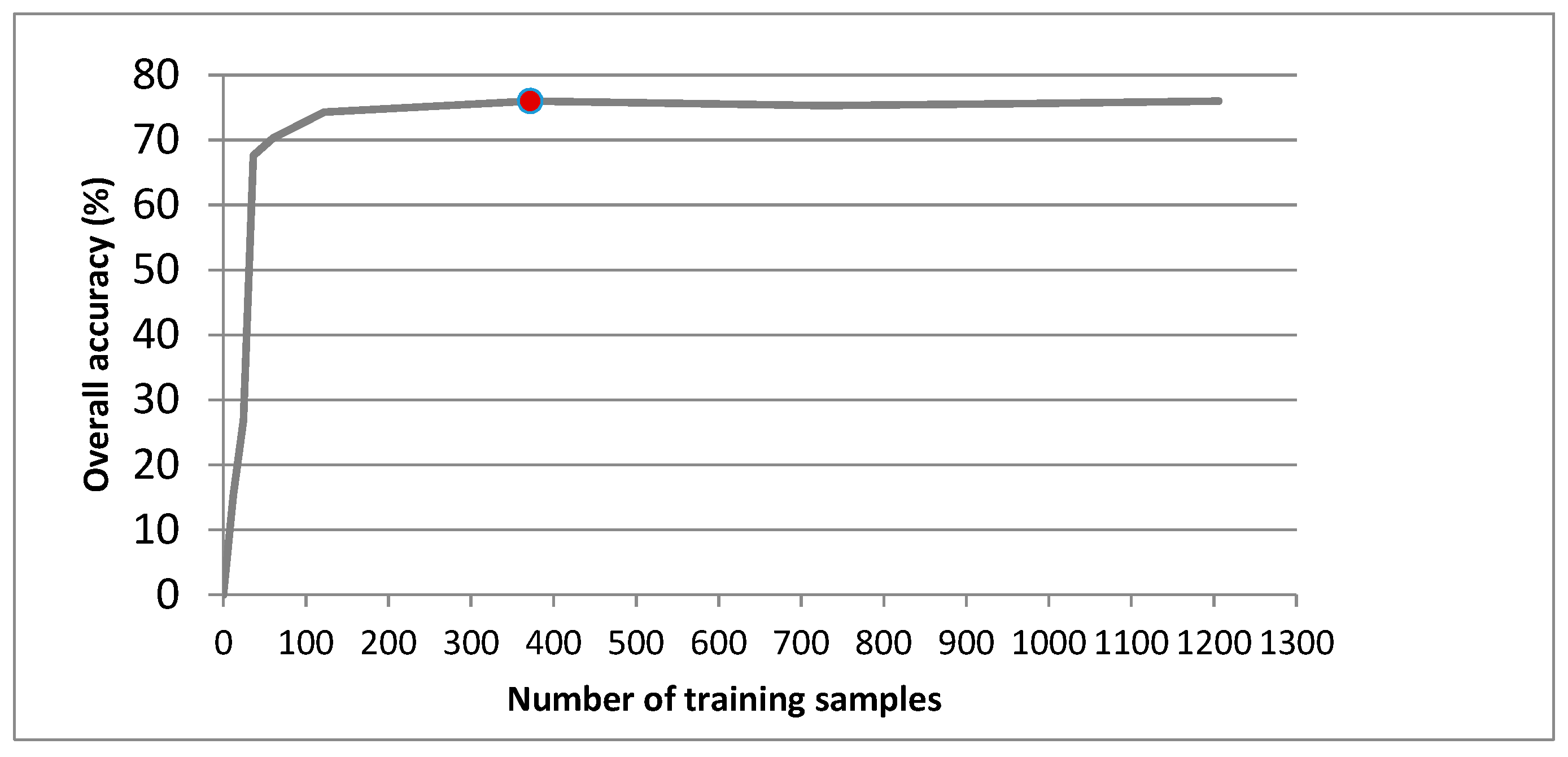
Figure 5.
The performance of the different sample sizes of the maximum likelihood classification with the Belgian grid as reference data. The graph shows that when the training size was large enough (more than 100 samples), the classification accuracy only slightly increased. At 372 samples (30% of the total training data), the overall accuracy (OA) reached a maximum. After that, it slightly decreased and finally increased slowly to reach the same OA.
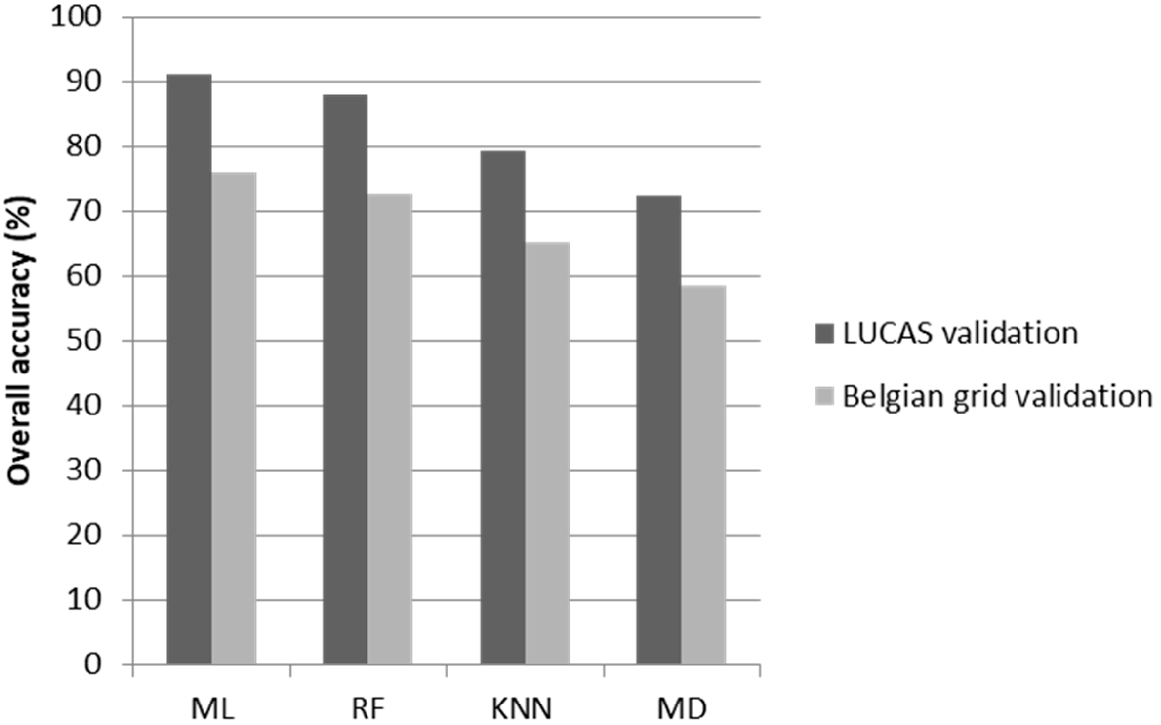
Figure 6.
Comparison of the OA of four classifiers: maximum likelihood (ML), random forest (RF), k-nearest neighbor (KNN), and minimum distance (MD). The graph shows that the performance of ML was the best regardless of the validation dataset used (OA = 91.1%, LUCAS validation; 76%, Belgian grid validation). The second-best classifier was RF (OA = 88%, 72.6%), followed by KNN (OA = 79.4%, 65.2%) and finally MD (OA = 72.4%, 58.4%).
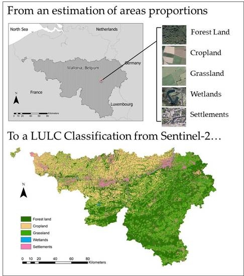
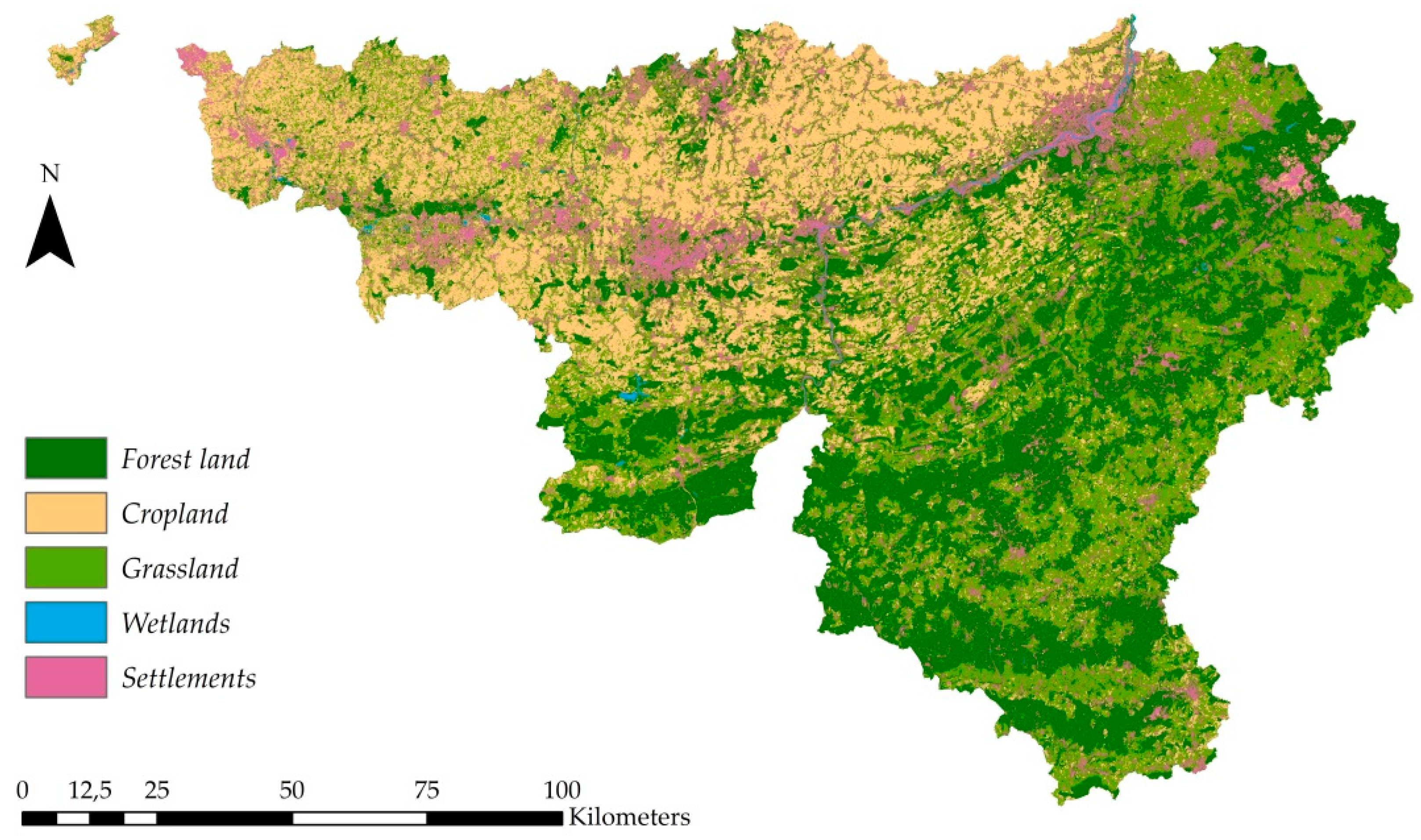
Figure 7.
Winter-spring-summer classification with four bands (B2, B3, B4, B8a) of Wallonia, Belgium. This classification was produced with Sentinel-2 data from the three-season mosaics (winter, spring, and summer 2016). The maximum likelihood classification algorithm was used with a training dataset of 372 samples (30% of the dataset). This classification reached an OA of 92.6%.
Table 1.
The dates of the images used to produce the three mosaics (winter, spring, and summer 2016).
Table 1.
The dates of the images used to produce the three mosaics (winter, spring, and summer 2016).
| | Winter | Spring | Summer |
|---|
| T31UDS | 27 December2016 | 16 March 2016 | 1 May 2016 | | 8 September 2016 |
| T31UES | 27 December 2016 | 12 March 2016 | 8 May 2016 | | 20 July 2016 |
| T31UFS | 4 December 2016 | 1 May 2016 | 8 May 2016 | | 25 September 2016 |
| T31UGS | 4 December 2016 | 12 March 2016 | 8 May 2016 | | 25 September 2016 |
| T31UER | 7 December 2016 | 12 March 2016 | 8 May 2016 | | 20 July 2016 |
| T31UFR | 4 December 2016 | 12 March 2016 | 1 May 2016 | 8 May 2016 | 25 September 2016 |
| T31UGR | 4 December 2016 | 8 May 2016 | 8 May 2016 | | 26 May 2016 |
| T31UFQ | 4 December 2016 | 8 May 2016 | 8 May 2016 | | 26 May 2016 |
Table 2.
Error tolerance of the four classifiers at a confidence level of 95% [
21,
22].
Table 2.
Error tolerance of the four classifiers at a confidence level of 95% [
21,
22].
| Classifiers | OA | Error Tolerance (±) |
|---|
| MLC | 0.911 | 0.019 |
| RF | 0.880 | 0.022 |
| KNN | 0.794 | 0.027 |
| MD | 0.724 | 0.030 |
Table 3.
The three-season confusion matrixes with four spectral bands (B2, B3, B4, and B8). (a) Winter classification; (b) spring classification; (c) summer classification. The reference data used here were the LUCAS validation dataset with 834 points. The summer classification yielded the best OA with 88.7%, followed by the spring classification (83.2%) and winter classification (73.9%).
| | | LUCAS Validation Dataset | | |
| Winter Classification (4 bands) | | F | C | G | W | S | Total | User’s Accuracy (%) |
| F | 152 | 7 | 7 | 8 | 5 | 179 | 84.9 |
| C | 5 | 139 | 37 | 0 | 22 | 203 | 68.4 |
| G | 12 | 20 | 146 | 3 | 11 | 192 | 76.0 |
| W | 0 | 3 | 0 | 96 | 2 | 101 | 95.0 |
| S | 18 | 32 | 12 | 14 | 83 | 159 | 52.2 |
| Total | 187 | 201 | 202 | 121 | 123 | 834 | |
| Producer’s Accuracy (%) | 81.2 | 69.1 | 72.2 | 79.3 | 67.4 | | |
| Overall Accuracy (%) | 73.86 | |
| | | LUCAS Validation Dataset | | |
| Spring Classification (4 bands) | | F | C | G | W | S | Total | User’s Accuracy (%) |
| F | 162 | 3 | 12 | 1 | 1 | 179 | 90.5 |
| C | 6 | 127 | 59 | 0 | 11 | 203 | 62.5 |
| G | 8 | 14 | 165 | 0 | 5 | 192 | 85.9 |
| W | 0 | 0 | 0 | 101 | 0 | 101 | 100.0 |
| S | 5 | 10 | 3 | 2 | 139 | 159 | 87.4 |
| Total | 181 | 154 | 239 | 104 | 156 | 834 | |
| Producer’s Accuracy (%) | 89.5 | 82.4 | 69.0 | 97.1 | 89.1 | | |
| Overall Accuracy (%) | 83.21 | |
| | | LUCAS Validation Dataset | | |
| Summer Classification (4 bands) | | F | C | G | W | S | Total | User’s Accuracy (%) |
| F | 171 | 1 | 4 | 1 | 2 | 179 | 95.5 |
| C | 4 | 157 | 39 | 0 | 3 | 203 | 77.3 |
| G | 0 | 18 | 170 | 0 | 4 | 192 | 88.5 |
| W | 0 | 0 | 0 | 100 | 1 | 101 | 99.0 |
| S | 0 | 6 | 9 | 2 | 142 | 159 | 89.3 |
| Total | 175 | 182 | 222 | 103 | 152 | 834 | |
| Producer’s Accuracy (%) | 97.7 | 86.2 | 76.5 | 97.0 | 93.4 | | |
| Overall Accuracy (%) | 88.7 | |
Table 4.
The three-season confusion matrixes with 10 spectral bands (B2, B3, B4, B5, B6, B7, B8, B8a, B11, and B12). (a) Winter classification; (b) spring classification; (c) summer classification. The reference data used here were the LUCAS validation dataset with 834 points. The summer classification yielded the best OA with 91.4%, followed by the spring classification (85.5%) and winter classification (80.0%).
| | | LUCAS Validation Dataset | | |
| Winter Classification (10 bands) | | F | C | G | W | S | Total | User’s Accuracy (%) |
| F | 160 | 1 | 7 | 3 | 8 | 179 | 89.4 |
| C | 2 | 152 | 28 | 0 | 21 | 203 | 74.9 |
| G | 9 | 20 | 146 | 1 | 16 | 192 | 76.0 |
| W | 2 | 0 | 3 | 90 | 6 | 101 | 89.1 |
| S | 7 | 20 | 12 | 1 | 119 | 159 | 74.8 |
| Total | 180 | 193 | 196 | 95 | 170 | 834 | |
| Producer’s Accuracy (%) | 88.9 | 78.8 | 74.5 | 94.7 | 70.0 | | |
| Overall Accuracy (%) | 80.0 | |
| | | LUCAS Validation Dataset | | |
| Spring Classification (10 bands) | | F | C | G | W | S | Total | User’s Accuracy (%) |
| F | 164 | 2 | 8 | 0 | 5 | 179 | 91.6 |
| C | 1 | 151 | 38 | 0 | 13 | 203 | 74.4 |
| G | 10 | 12 | 156 | 0 | 14 | 192 | 81.3 |
| W | 3 | 0 | 0 | 94 | 4 | 101 | 93.1 |
| S | 1 | 7 | 3 | 0 | 148 | 159 | 93.1 |
| Total | 179 | 172 | 205 | 94 | 184 | 834 | |
| Producer’s Accuracy (%) | 91.6 | 87.8 | 76.1 | 100.0 | 80.4 | | |
| Overall Accuracy (%) | 85.5 | |
| | | LUCAS Validation Dataset | | |
| Summer Classification (10 bands) | | F | C | G | W | S | Total | User’s Accuracy (%) |
| F | 174 | 0 | 1 | 0 | 4 | 179 | 97.2 |
| C | 1 | 182 | 12 | 0 | 8 | 203 | 89.7 |
| G | 0 | 21 | 161 | 0 | 10 | 192 | 83.9 |
| W | 2 | 0 | 0 | 96 | 3 | 101 | 95.0 |
| S | 0 | 6 | 4 | 0 | 149 | 159 | 93.7 |
| Total | 177 | 209 | 178 | 96 | 174 | 834 | |
| Producer’s Accuracy (%) | 98.3 | 87.1 | 90.4 | 100.0 | 85.6 | | |
| Overall Accuracy (%) | 91.4 | |
Table 5.
The confusion matrixes for the multidate classification with 4 (B2, B3, B4, and B8) and 10 spectral bands (B2, B3, B4, B5, B6, B7, B8, B8a, B11, and B12). (a) Winter-spring-summer classification with 4 bands; (b) spring-summer classification with 4 bands; (c) winter-spring-summer classification with 10 bands; (d) spring-summer classification with 10 bands. The reference data used here were the LUCAS validation dataset with 834 points. The winter-spring-summer classification with 4 bands yielded the best OA with 92.6%. It was followed by the spring-summer classification with 4 bands (91.5%) and the spring-summer classification with 10 bands (90.2%). The winter-spring-summer classification with 10 bands yielded the worst OA (86.8%).
| | | LUCAS Validation Dataset | | |
| Winter-Spring-Summer (4 bands) | | F | C | G | W | S | Total | User’s Accuracy (%) |
| F | 172 | 4 | 0 | 1 | 2 | 179 | 96.1 |
| C | 1 | 184 | 17 | 0 | 1 | 203 | 90.6 |
| G | 0 | 17 | 173 | 0 | 2 | 192 | 90.1 |
| W | 0 | 0 | 0 | 97 | 4 | 101 | 96.0 |
| S | 0 | 8 | 4 | 1 | 146 | 159 | 91.8 |
| Total | 173 | 213 | 194 | 99 | 155 | 834 | |
| Producer’s Accuracy (%) | 99.4 | 86.4 | 89.2 | 98.0 | 94.2 | | |
| Overall Accuracy (%) | 92.6 | |
| | | LUCAS Validation Dataset | | |
| Spring-Summer (4 bands) | | F | C | G | W | S | Total | User’s Accuracy (%) |
| F | 174 | 0 | 1 | 1 | 3 | 179 | 97.2 |
| C | 1 | 175 | 23 | 0 | 4 | 203 | 86.2 |
| G | 0 | 21 | 168 | 0 | 3 | 192 | 87.5 |
| W | 0 | 0 | 0 | 98 | 3 | 101 | 97.0 |
| S | 0 | 8 | 2 | 1 | 148 | 159 | 93.1 |
| Total | 175 | 204 | 194 | 100 | 161 | 834 | |
| Producer’s Accuracy (%) | 99.4 | 85.8 | 86.6 | 98.0 | 91.9 | | |
| Overall Accuracy (%) | 91.5 | |
| | | LUCAS Validation Dataset | | |
| Winter-Spring-Summer (10 bands) | | F | C | G | W | S | Total | User’s Accuracy (%) |
| F | 162 | 4 | 2 | 0 | 11 | 179 | 90.5 |
| C | 1 | 182 | 12 | 0 | 8 | 203 | 89.7 |
| G | 1 | 26 | 156 | 0 | 9 | 192 | 81.3 |
| W | 13 | 1 | 0 | 77 | 10 | 101 | 76.2 |
| S | 0 | 11 | 1 | 0 | 147 | 159 | 92.5 |
| Total | 177 | 224 | 171 | 77 | 185 | 834 | |
| Producer’s Accuracy (%) | 91.5 | 81.3 | 91.2 | 100.0 | 79.5 | | |
| Overall Accuracy (%) | 86.8 | |
| | | LUCAS Validation Dataset | | |
| Spring-Summer (10 bands) | | F | C | G | W | S | Total | User’s Accuracy (%) |
| F | 169 | 1 | 1 | 0 | 8 | 179 | 94.4 |
| C | 1 | 188 | 10 | 0 | 4 | 203 | 92.6 |
| G | 0 | 23 | 156 | 0 | 13 | 192 | 81.3 |
| W | 2 | 0 | 0 | 88 | 11 | 101 | 87.1 |
| S | 0 | 6 | 2 | 0 | 151 | 159 | 95.0 |
| Total | 172 | 218 | 169 | 88 | 187 | 834 | |
| Producer’s Accuracy (%) | 98.3 | 86.2 | 92.3 | 100.0 | 80.7 | | |
| Overall Accuracy (%) | 90.2 | |
Table 6.
Comparison of land areas in kha from the three best classification products (winter-spring-summer with 10 bands, spring-summer with 4 bands, and summer with 10 bands) to the Greenhouse Gas (GHG) Inventory Report and the Corine Land Cover 2012. (a) The winter-spring-summer classification with 4 bands (best OA reached, 92.6%); (b) the spring-summer classification with 4 bands (second-best OA, 91.5%); (c) the summer classification with 10 bands (third-best OA, 91.4%). All the land areas were within the same range except the wetlands, which varied from 2.86 kha (winter-spring-summer with 10 bands) to 16.00 kha (GHG Inventory Report of 2016).
| | Winter-Spring-Summer (4 bands) Classification | GHG Inventory Report | CLC12 |
| Classes | kha | kha | kha |
| Forest Land | 570.91 | 556.40 | 516.74 |
| Cropland | 428.78 | 456.40 | 588.98 |
| Grassland | 464.33 | 400.40 | 321.41 |
| Wetlands | 6.32 | 16.00 | 10.10 |
| Settlements | 225.83 | 258.60 | 253.22 |
| Total | 1696.17 | 1687.80 | 1690.44 |
| | Spring-Summer (4 bands) Classification | GHG Inventory Report | CLC12 |
| Classes | kha | Kha | Kha |
| Forest Land | 570.99 | 556.40 | 516.74 |
| Cropland | 424.85 | 456.40 | 588.98 |
| Grassland | 473.91 | 400.40 | 321.41 |
| Wetlands | 7.42 | 16.00 | 10.10 |
| Settlements | 219.14 | 258.60 | 253.22 |
| Total | 1696.32 | 1687.80 | 1690.44 |
| | Summer (10 bands) Classification | GHG Inventory Report | CLC12 |
| Classes | Kha | Kha | Kha |
| Forest Land | 575.90 | 556.40 | 516.74 |
| Cropland | 451.45 | 456.40 | 588.98 |
| Grassland | 397.08 | 400.40 | 321.41 |
| Wetlands | 6.60 | 16.00 | 10,10 |
| Settlements | 265.29 | 258.60 | 253.22 |
| Total | 1696.32 | 1687.80 | 1690.44 |


