Abstract
Urban ecosystem services (ES) contribute to the compensation of negative effects caused by cities by means of, for example, reducing air pollution and providing cooling effects during the summer time. In this study, an approach is described that combines the regional biotope and land use data set, hemeroby and the accessibility of open space in order to assess the provision of urban ES. Hemeroby expresses the degree of naturalness of land use types and, therefore, provides a differentiated assessment of urban ES. Assessment of the local capacity to provide urban ES was conducted with a spatially explicit modeling approach in the city of Halle (Saale) in Germany. The following urban ES were assessed: (a) global climate regulation, (b) local climate regulation, (c) air pollution control, (d) water cycle regulation, (e) food production, (f) nature experience and (g) leisure activities. We identified areas with high and low capacity of ES in the urban context. For instance, the central parts of Halle had very low or no capacity to provide ES due to highly compact building styles and soil sealing. In contrast, peri-urban areas had particularly high capacities. The potential provision of regulating services was spatially limited due to the location of land use types that provide these services.
1. Introduction
Urbanization is globally one of the key development processes of the 21st century [1]. Currently, about 55% of the world’s population lives in urban areas [2], which highlights the trend that living in urban contexts will be the predominant form of human life in the future. A highly relevant consequence is an increase in conflicts concerning open and particularly green space, which provides the highest degree and a broad range of urban ecosystem services (ES) [3]. The ES concept represents a theoretical and anthropocentric basis for the social, ecological and economic valuation of nature, addressing the direct and indirect benefits that ecosystems provide to society spanning from biogeophysical structures and landscape patterns, to functions, services and economically assessable impacts on societies [4,5,6,7]. Different evaluation frameworks, such as those suggested by Diaz et al. (2015) [8] in the context of the Intergovernmental Science-Policy Platform on Biodiversity and Ecosystem Services (IPBES) describe how drivers and cause-effect relationships should be reflected. However, the cascade model suggested by Haines-Young and Potschin (2010) [6], adopted by “The Economics of Ecosystems and Biodiversity” (TEEB 2010) [7] and implemented in the context of the “Common International Classification of Ecosystem Services” [9] best illustrates how to interpret and connect the interactions between humans and nature to ensure the sustainable conservation of biodiversity and provision of essential ES.
Urban ES can be considered as a subcategory of ES that incorporate the particular character of urban landscapes, which are much more dominated by artificial structures, but also areas dedicated to restoration and nature conservation to provide ES close to where these are demanded [10]. Environmental problems like heat stress, poor air quality and noise can cause health problems and ES contribute to reduce these negative effects by, for example, the absorption of sound waves by vegetation barriers [11] or air filtration by trees [12]. More frequent extreme events such as droughts, floods or storms increase the need to improve ES to buffer or compensate negative effects [13].
Even though there is often a strong anthropogenic disturbance, biodiversity in cities can be high due to niches, complex land use mosaics, and small-scale structures [14]. In addition, urban cultural ES, such as nature experiences, depend on biodiversity [15]. A major challenge of nature conservation is therefore to preserve the biological diversity of the different urban land use types [16].
In view of ongoing urbanization and urban density, it is a central task to identify innovative approaches and tools to assess urban ES. Ziter (2016) [17] identified in a literature analysis that 97 of 133 (approx. 73%) urban ES assessments were related to regulating ES; mainly regarding carbon sequestration and local climate. However, the capacity of urban ecosystems to provide services to society has not been well researched, as assessment data sources such as CORINE (Coordination of Information on the Environment) land cover do not allow for differentiation of the structures and functions of urban niches and biotopes [18]. Consequently, less than 10% of all ES publications have dealt thus far with urban ES, although their number has been increasing recently [3]. The spatial distribution of urban ES is also of importance because green spaces are often unequally distributed. Often, population groups with low socio-economic status are disadvantaged by limited access to public green spaces of high quality and they are, therefore, affected by negative environmental effects [19]. Environmental justice and the development of green space to keep and develop good living conditions in cities will be a key challenge in future urban development.
The aim of this study was to showcase how to improve the mapping of urban ES using a study area in the city of Halle (located in the Federal State Saxony–Anhalt), Germany, as an example. In our study, we explored the opportunities to base the assessment on a data set that provides more detailed information on the ecosystem character or land uses, called “biotope and land use mapping” compared to the single use of land cover data sets, e.g., CORINE land cover data. Furthermore, we explored the opportunities of using the hemeroby concept that is based on the degree of human disturbance [20,21]. We suggest an adjustment of the hemeroby concept to better express the status of the mapped ecosystems in terms of degradation and disturbance, but also with regard to better restoration or creation of biotopes in an urban context [22]. The degree of ecosystem transformation in urban areas can be measured by the proportion of sealed and built-up land [23]. The sealing describes the sum of paved areas, asphalt and building construction, while built-up land includes all forms of houses and buildings [24]. The proportion of vegetation cover indicates the degree of naturalness of the area [23]. Finally, we included information on ownership of the urban areas by using the proxies of visibility and accessibility (private–public space) to address the aspect of recreational services due to the fact that the provision of cultural ES is dependent on accessibility [4].
2. Materials and Methods
2.1. Study Area
Halle (Saale) (51°29′49.129″ N 11°58′7.69″ E) is one of the largest cities of the state Saxony–Anhalt with 238,321 inhabitants and a total area of 13,502 hectares (Figure 1). Within an average diameter of 15 to 17 km, the city is characterized by a compact urban structure. As a former highly industrialized area in the period of the German Democratic Republic, the city has been successful in improving the quality of the built-up and natural environment today and has thus achieved a higher quality of living for its inhabitants [25]. Green corridors close to the city have important ecological and recreational functions and serve as a regional planning target [26]. The Saale river (especially the Saale–Elster meadow and Saale–Elster floodplain), as a green belt connecting Halle with Leipzig, historic parks and the forest heathland “Dölauer Heide” contribute to improving the green infrastructure of the city.
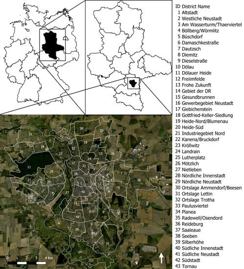
Figure 1.
Map of the city of Halle with district names (in the geographical information system software QGIS, version 2.18; Google Maps 2018; German Federal Agency for Cartography and Geodesy—BKG 2018 [27]). Halle is located in the Federal State Saxony–Anhalt (top right) of Germany (top left). The Saale–Elster meadow and Saale–Elster floodplain are mainly located in the districts Saaleaue, Böllberg, Kröllwitz, Trotha and Planena.
2.2. Spatial Assessment Tools
For mapping and assessing the ES of the city of Halle, we used the web-based modeling platform GISCAME (GIS = geographic information system, CA = cellular automaton, ME = multi criteria evaluation) that was developed to support planning processes by simulating and assessing alternative land use scenarios [28]. Furthermore, GISCAME can be used to include information about environmental and landscape properties, such as climatic or topographical data, in the impact assessment. GISCAME consists of a combination of cellular automata with GIS functions and a multi-criteria assessment. The multi-criteria assessment cumulates the particular contribution of single land uses up to regional capacities to provide ES based on indicators and mathematical normalization [29]. The normalized values range from zero (no ES provision) to 100 (highest ES provision) in relation to other ES for the region. As output, maps with land cover types and the related capacities for ES provision are created. Furthermore, the relationship between the differently assessed ES are reflected in a spider chart, and trade-offs between the different ES can be assessed in different land use scenarios. See Fürst et al. (2010) [28] and GISCAME (2018) [30] for more information on GISCAME.
For coding the areas, the field calculator in the attribute table of an open access geographical information system, QGIS (version 2.18), was used. After the coding, the attribute table contains different numerical codes per spatial unit, which explains the hemeroby, land use type and accessibility of the spatial unit. Finally, codes have been assigned to different colors and presented as a map. This map was exported to GISCAME. In this study, GISCAME was used for the ES assessment and to present the results in capacity maps. Additionally, the spider diagram in GISCAME was chosen to present the relationship between the ES.
2.3. Data Base and Re-Classification—Combination of the Regional Biotope and Land Use Data Set, Hemeroby and Accessibility
Different assessment methods, formulas and data types were necessary to adapt the hemeroby concept to the urban context in order to streamline the different ES provision levels and prepare data for GISCAME and QGIS (Figure 2). Seven regulating, cultural and provisioning ES were considered in the ES assessment (see Section 2.4 for more details). At first, the hemeroby concept was translated into the urban context by using the degree of sealed area and the degree of tree cover (“urban hemeroby” in Figure 2). The regional biotope and land use data set (BTNT) was used as the spatial basis for the study area. With regard to cultural ES, accessibility was also taken into account. In order to normalize all ES in GISCAME and use the values for capacity maps in QGIS in a later step, formulas in combination with information from Burkhard et al. (2014) [31] and Walz and Stein (2014) [32] were used. Regarding provisioning ES, a five-point Likert scale was chosen.
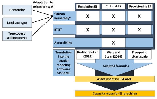
Figure 2.
Overview of the methodological framework. A ticked box means that the respective approach was used to assess the ecosystem service (ES). BTNT = Regional biotope and land use data set. GISCAME: GIS = geographic information system, CA = cellular automaton, ME = multi criteria evaluation.
All areas were classified with the field calculator in the attribute table in QGIS by use of an integrative code with three digits:
- First digit: the hemeroby of the area (Section 2.3.1)
- Second digit: the biotope or land use type of the area (Section 2.3.2)
- Third digit: the accessibility of urban nature to the public (Section 2.3.3).
Hemeroby is an approach to describe the closeness to nature and the cultural influence of vegetation. It was first developed by the Finnish biologist Jalas (1955) [20] and transferred to entire ecosystems by Sukopp (1972) [21]. The four-degree scale from Jalas (1955) [20], which describes the gradient from natural to artificial areas, is extended by three degrees in Blume and Sukopp (1976) [33]. Our coding resulted in a total of 64 different classes for the subsequent assessment of urban ES provision capacities.
2.3.1. Classification of Land Use Classes into Hemeroby Degrees (1st Digit)
Based on the concepts presented by Jalas (1955) and Blume and Sukopp (1976) [20,33] (Table 1), we adjusted the hemeroby concept to better address the ecological contributions of urban areas for all types of use in the built-up area (green and open spaces, residential and mixed areas, industrial and commercial areas, allotments, allotment gardens, traffic areas, sports, leisure and camping facilities and other areas of the built-up area). Therefore, the hemeroby degrees from “β-euhemerob—moderate-strong human impact” to “metahemerob—excessively strong human impact” were sub-classified in our approach (see Table 1). These urban land use types have been classified according to the indicators “degree of sealing” and “degree of tree cover.” As a result, green areas with the same sealing and tree cover ratio as residential areas are also assigned to the same hemeroby degree and, thus, the hemeroby assessment can only be compared for the respective biotope or land use type.

Table 1.
Hemeroby degrees according to Jalas (1955) and Blume and Sukopp (1976) [20,33] and adapted degrees in the urban context for our analysis. The urban degree names follow Schlüter (1999) [34].
Soil sealing degree and tree/wood cover were taken from the biotope and land use data set [35], where for each built-up area, four different sealing types and four different tree cover types have been mapped by the Environmental Protection Agency of Saxony–Anhalt (Figure 3). For instance, areas with a low degree of sealed area (<25%) and a high degree of tree cover (>50%) were assigned to hemeroby degree 3 (Table 2). Completely sealed areas, such as roads and other built-up areas, were assigned to hemeroby degree 10 (artificial), as the entire biocoenosis in this area is destroyed. Forest heathlands, such as the Dölauer Heide, were grouped in degree 1 (conditionally natural) and groups of trees, hedges and bushes were assigned to degree 2 (close to nature). Extensively used meadows were assigned to degree 3 (conditionally close to nature). Naturally occurring dry grasslands were assigned to hemeroby degree 1.
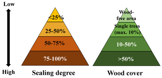
Figure 3.
Steps of the sealing degree and wood cover according to the regional biotope and land use data set for built-up areas [35].
Table 2.
Hemeroby degrees in the context of a built-up area (the urban degree names follow Schlüter 1999; LAU 1992 [34,35]).
2.3.2. Land Use/Land Cover Data Sets—Biotope and Land Use Mapping Data (2nd Digit)
We adopted the regional biotope and land use data set (BTNT) of the Environmental Protection Agency of Saxony–Anhalt for assessing urban ES with a closer consideration of biotopes, niches and habitats in the context of the city of Halle. The available BTNT was mapped by using color-infrared aerial photographs of the State of Saxony–Anhalt on a scale of 1:10,000 as basis. The BTNT originates from 2009. Its replication was planned for 2016, but was not yet available for this study. The BTNT layer holds seven different main mapping units ([35]; Table 3).
Table 3.
The seven main mapping units of the regional biotope and land use data set [35].
The main mapping units were divided into 42 subunits. The subunits describe dominating species, structural features (e.g., scrub encroachment) and site characteristics (e.g., hydrological properties). Since built-up areas are the focus of this study, this mapping unit was further specified [35]:
- (7a)
- Built-up area 1: green and open areas of the built-up area
- (7b)
- Built-up area 2: residential and mixed-use areas
- (7c)
- Built-up area 3: industrial and commercial areas
- (7d)
- Built-up area 4: allotment gardens
- (7e)
- Built-up area 5: traffic areas
- (7f)
- Built-up area 6: sports and leisure facilities/camping
- (7g)
- Remaining built-up areas (not further classified)
Water as a mapping unit was excluded in further analysis because this study focused on terrestrial ecosystems.
2.3.3. Division into Private or Public Accessible Urban Area (3rd Digit)
The biotope and land use types with recreational services and public access in our study were parks, cemeteries, grassland, orchards, other urban green spaces, forests, groups of trees and water bodies [36]. However, there are huge differences in the spatial differentiation of their quality across cities: although private gardens and public green spaces provide similar ES, they cannot be considered equally in their value for recreation due to restricted access. The area of private urban green spaces can amount to as much as 45% of a city’s total green space [37] so that half of a city is not usable for public recreation. Socially disfavored urban districts tend to be either less well equipped with urban green recreation spaces or, even if they hold recreationally valuable green urban spaces, these are not easy to reach due to long walking distances [38]. We included the accessibility of urban nature into its value for recreation according to Grunewald et al. (2017) [36]. They presented a list of green space with recreational functions and accessibility for the public in Germany. In addition, in order to determine the general accessibility of green spaces in residential areas, inherent information from BTNT on the housing types was used. Furthermore, we examined the housing types in orthophotos and confirmed accessibility by the different housing types on site.
BTNT residential areas that were mapped as “modern perimeter development” and “high-rise buildings” were classified as “public”, since the green spaces for those settlement types are mainly accessible for public (we could not include information on land use intensity). For example, the Neustadt of Halle is characterized by “high-rise buildings” and has a large area of public free space [39]. The urban nature of the remaining settlement types, like “row houses” and “old perimeter development” in the city center is, at least in our case study, mainly not open to the public and was thus classified as “private”. Exemplary orthophotos of building types and accessibility of green spaces can be viewed in Appendix A.
2.4. Selection of Urban Ecosystem Services
In this study, seven different ES and their provisions in the city of Halle (Saale) were mapped and assessed. Their selection was based on literature (e.g., [37,40,41]; see Table 4) emphasizing that these ES play an outstanding role in our particular urban context for human health, physical and mental well-being. Four regulating ES (global climate regulation, local climate regulation, air pollution control and water cycle regulation) and two ES (“rest/nature experience” and “social interaction/leisure”) were selected. Furthermore, due to the increasing scientific discussion about agriculture and gardening in urban areas, the ES “food supply” was included. The terminology follows TEEB (2010) [7].
Table 4.
The selected ecosystem services (ES) and its relevance for human health and physical and mental well-being in the urban context. More information on the specific ES can be found in Appendix B.
2.5. Assessment Approach of Urban Ecosystem Services
In the following sections (Section 2.5.1, Section 2.5.2 and Section 2.5.3), the assessment method and related formula for each ES class is explained.
2.5.1. Regulating Ecosystem Services
For the assessment of regulating ES, the soil sealing and tree/woody space coverage based on the hemeroby classification (see Section 2.3.1) and the land use types from BTNT (see Section 2.3.2) were primarily used because public accessibility does not play an essential role for their provision. Highly natural ecosystems, such as forests, provide the highest level of regulating ES [53], and with increasing cultural influence on the ecosystem, capacities to provide regulating ES are decreasing [31]. Table 5 summarizes how the urban hemeroby degrees are converted into normalized hemeroby index values for the assessment in GISCAME. The normalized scale stretches from 0 (lowest/no provision) to 100 (highest provision).
Table 5.
Urban hemeroby degrees converted to urban normalized hemeroby index values for the ecosystem services assessment. Value 100 = highest ecosystem service capacity; 0 = lowest/no ecosystem service capacity.
In the following, the hemeroby index values presented in Table 5 were used as an initial value which reflects the tendency to the provision of regulating ES. However, the same hemeroby degrees would be assigned to different land use types that are not comparable with regard to ES provision. In order to bring hemeroby into an ES context, the “Burkhard Matrix” [31] was used. This matrix represents a qualitative assessment of the capacity of ES provided by different land use types. The assessment scale ranges from 0 (no relevant capacity) to 5 (very high relevant capacity). Evaluations of ES capacities refer to a central European normal landscape [31].
The following Formula (1) was used for calculating the regulating ecosystem services:
HI − ((5 − BM):10) × HI = VR
HI = Index value urban hemeroby (see Table 5)
BM = Value of ES capacity in the Burkhard Matrix (see Table 6)
Table 6.
The biotope and land use data set classified according to the “Burkhard Matrix” (BM) and its devaluation (D) in our context. Burkhard et al. (2014) [31] classified all biotope and land use types of a central European landscape using the following range: 5 = very high capacity to provide a specific ecosystem service; 0 = no capacity to provide a specific ecosystem service. Water (mapping unit 4) was excluded.
VR = Value for regulating ES
Each biotope or land use type that was evaluated with the highest capacity in the Burkhard Matrix [31] remains as the normalized hemeroby index value presented in Table 5. Biotope and land use type with lower capacity in Burkhard et al. (2014) [31] were devalued stepwise by 10% per lower digit, which finally reflected the index value for each regulatory service after the devaluation. Table 6 presents all combinations with the devaluation ((5 − BM):10) based on the Burkhard Matrix and the normalized hemeroby index.
For example, green urban areas are assessed with the value 2 in the Burkhard Matrix for “global climate regulation”, while residential and mixed-used areas are assessed with 0. Therefore, we devalued the urban hemeroby index value by 30% for green urban areas and for residential and mixed-used areas by 50%. The remaining values then resulted in the index value for the regulating ES “global climate regulation”. In the following is an example for a green urban area and for a residential area with an urban hemeroby index value of 4. In Section 3.2, the results of all ES and index values are presented.
- Examples:
- HI of hemeroby degree 4 = 70
- BM for green urban areas = 2
- BM for residential and mixed-used areas = 0
- Green urban area: 70 − ((5 − 2):10) × 70 = 49
- Residential and mixed-used area: 70 − ((5 − 0):10) × 70 = 35
2.5.2. Cultural Services
Regarding cultural ES, we focused on recreational services since urban open spaces are mainly used for recreation activities and the need for places to rest, and compared to rural areas, are very high [31,54]. In contrast to the assessment of regulating ES, non-natural parks can also have a high potential to provide recreational services, as they are characterized by open vegetation structures and offer a lot of space and structures for social interaction and leisure activities. Therefore, it makes sense to assess two different forms of recreation: (a) a recreation service which describes the potential for rest and nature experiences and (b) a recreation service which describes the potential for social interaction and leisure activities.
The assessment of the “rest and nature experience” was based on the urban hemeroby index (Table 7), referring to the hemeroby rating suggested by Walz and Stein (2014) [32], to provide a value depending on the biotope and land use type. Since degrees 1 and 2 of the Walz and Stein (2014) [32] assessment occur only very rarely in our urban context, degree 3 reflects the most natural area.
Table 7.
Index values for the assessment of “rest and nature experiences.” Water (mapping unit 4) was excluded because the analysis focuses on terrestrial ecosystems. Agriculture (mapping unit 6) was regarded as not accessible for the public. The devaluation of the hemeroby index value was based on the difference to hemeroby degree 3 (most natural areas) according to Walz and Stein (2014) [32].
The following Formula (2) was used for calculating the ecosystem service “rest and nature experience”:
HI − (DH:10) × HI = HB
HI = Index value urban hemeroby (see Table 3)
DH = Difference to hemeroby degree 3 according to Walz and Stein (2014) [32]
HB = Hemeroby value of the area depending on the biotope or land use type
- Examples:
- HI of hemeroby 4 = 70
- DH for green urban areas = 1
- DH for residential and mixed-used areas = 4
- Green urban area: 70 − (1:10) × 70 = 63
- Residential and mixed-used area: 70 − (4:10) × 70 = 38
All biotope and land use types that have been evaluated at degree 1–3 keep the full hemeroby index value. All other biotope and land use types are devalued by 1 per degree (see Table 7). In addition to hemeroby, the accessibility of the biotope and land use types is involved in the assessment of recreational ES. Thus, all areas that are not open to the public are rated with the index value 0 (no provision of the cultural ES). Since agricultural areas were rated as “private”, they are not considered to provide recreational services. Haase et al. (2012) [55] also mentioned that agricultural areas are not visited for recreation.
For the assessment of the ES “social interaction and leisure activities,” an index value on a scale of 0 to 100 was used (Table 8). The assessment and the index values were based on a walking survey though Halle (Saale) and the examination of orthophotos. Areas with hemeroby degree 5 (conditionally unnatural) received the highest value (100), as these areas provide a well-balanced mixture between natural and artificial landscapes and they are, therefore, suitable for recreational sports and other leisure activities (Table 8). Furthermore, those areas provide a lot of space for social interaction, but because of their low sealed area, they still have a high relationship to urban nature. Open spaces and green areas of hemeroby degree 5 and 6 often contain playgrounds, sports facilities, benches and seating areas [56] and are, therefore, most valuable for social interaction and leisure activities. This was also the result found by Garcia-Llorente et al. (2012) [57], where respondents rated ecosystems with moderate cultural influence better for the provision of cultural services than natural ecosystems. Therefore, the hemeroby degrees 1–4 are devalued by 10 index points per degree so that hemeroby degree 1 has an index value of 60. In contrast to nature experiences, near-natural forests are less suitable for most leisure activities and offer fewer opportunities for social interaction. Another reason for the devaluation is the lack of playgrounds, playground equipment, sports facilities or other equipment and structures used for leisure and sports activities. Furthermore, many near-natural areas of the city of Halle have been designated as protected areas. Therefore, they are less suitable for many social and leisure activities, which also justify a devaluation. For example, music is not allowed to be played in the Dölauer Heide nature reserve [58] and any sporting, tourist or other event is prohibited in the Forstwerder nature reserve, located in the Halle district Trotha [59]. Hemeroby degrees 6–10 are also devalued by 10 index points per degree since the suitability for leisure and sports decreases with increasing housing area.
Table 8.
Index values for the assessment of “social interaction and leisure activities” for the assessment in GISCAME. All private areas were valuated with “no provision of this ecosystem service”. Value 100 = highest ecosystem service capacity; 0 = lowest/no ecosystem service capacity.
2.5.3. Food Supply
The assessment of food supply is more challenging with BTNT and hemeroby degrees. Allotment gardens are characterized by diverse, not purely agricultural usage [60]. In 2004, the Federal Supreme Court of Germany ruled that at least one third of all allotment gardens must be used for the cultivation of fruit and vegetables [61]. However, the exact percentage of cultivated area per garden is very different, which also makes it difficult to make an accurate assessment. The BTNT does not provide information on the current usage of the allotment gardens. Another problem was that areas used for urban gardening do not have their own land use classification and therefore cannot be separated from green areas or other open spaces. Consequently, for the evaluation of the ES “food supply”, we mapped only capacity degrees in food supply using a five-point Likert scale from very low or no provision to very high provision, which was then subsequently translated to the scale 0 (no provision) to 100 (highest provision) in 25 value point steps (Table 9). For example, the potential for food from conventional agricultural area is “very high” and the potential of urban settlements such as the old town of Halle and industrial areas is “very low” (or no provision). All extensively used orchards and areas used for urban gardening have “high” potential. Hemeroby degrees 1–3 have a moderate capacity to provide food because they have a higher potential for the provision of edible wild plants than rather unnatural areas. Areas with “low” potential are characterized by increased sealing and a lower tree cover but still able to provide partially edible wild plants such as blackberries.
Table 9.
Five-point Likert scale for the ecosystem service “food supply”. Value 100 = highest ecosystem service capacity; 0 = lowest/no ecosystem service capacity.
3. Results
The following sections present the areas allocated to the three-digit classes (Section 3.1) and the results from the integrated ES assessment and mapping approach for Halle (Section 3.2). Here, based on the matrix (Section 3.2.1), we show a spider diagram that reflects the average index value for each assessed ES in Halle. In addition, the ES capacity maps from the index values are presented (Section 3.2.2).
3.1. Spatial Statistics—Areas Allocated to BTNT, Hemeroby and Accessibility
The areas allocated to the different BTNT, hemeroby degrees and accessibility in Halle are presented in Table 10. The proportion of forest in Halle is 10.42%, where 8.77% was allocated to the hemeroby degree 1. Herbaceous vegetation is found on 16.27% of Halle’s urban area. Of this classification, 0.19% was allocated to hemeroby degree 1, as this is natural dry grassland. About 2.43% is natural grassland, which is located particularly in the Saale floodplain south of the Silberhöhe district and has been assigned to hemeroby degree 3.
Table 10.
Hemeroby of the regional biotope and land use data types (BTNT) in percentage of the total area of Halle.
About 21.29% of Halle’s urban area is agricultural land or land used for commercial horticulture. Due to the focus on built-up areas in this work, both land uses were combined into the “agriculture” group and assigned to hemeroby degree 5. Green and open spaces in the built-up area account for 3.04% of the total area from Halle. It can be seen that around two-thirds of the green and open spaces are characterized by a high degree of wood cover and low sealing degree. Only one-third of the area has low cover or is heavily sealed. With regard to the total percentage value of green and open spaces, it should be noted that parts of green spaces in the BTNT are classified as groups of trees or herbaceous vegetation and have therefore not been added. This explains the relatively small percentage of green and open spaces, but underlines the accuracy of the data set. Industrial and commercial areas account for 9.3% of the municipal area in Halle. This fact shows that even commercial and industrial areas can contribute to ES provision to a small share.
3.2. Results of the Ecosystem Service Assessment
3.2.1. Index Values of Ecosystem Services
In the following, the results from the differentiation between hemeroby degrees and ES capacity by different biotope and land use types are shown (Table 11, Table 12 and Table 13). The index values have been used for the ES assessment in GISCAME. For example, the highest capacity to provide global climate regulation, local climate regulation, air pollution control, water cycle regulation and nature experience is provided by forest and woody plants with hemeroby degree 1 (conditionally natural) and 2 (close to nature). For water cycle regulation, none of the land use types can provide the maximum value of 100 due to a medium to low ES provision potential for the assessed land use types according to Burkhard et al. (2014) [31]. For food supply, the highest index values are provided for agriculture as a conditionally unnatural area (hemeroby degree 5), but also allotment gardens as conditionally close to nature (hemeroby degree 3), semi-natural (hemeroby degree 4) and conditionally unnatural (hemeroby degree 5) have a high capacity to provide food. For recreational services, agricultural area has no capacity since it was considered as private area in the analysis.
Table 11.
Index values for regulating ecosystem services (ES) global climate regulation, local climate regulation, air pollution control, water cycle regulation for the most common biotope or land use type and each hemeroby degree. Value 100 = highest ecosystem service capacity; 0 = lowest/no ecosystem service capacity.
Table 12.
Index values for “nature experience” and “social interaction and leisure faculties” for the most common biotope or land use type and each hemeroby degree. Value 100 = highest ecosystem service capacity; 0 = lowest/no ecosystem service capacity.
Table 13.
Index values for food supply for the most common biotope or land use type and each hemeroby degree. Value 100 = highest ecosystem service capacity; 0 = lowest/no ecosystem service capacity.
Based on the matrix, a spider diagram was compiled in GISCAME which shows the average index value for each assessed ES in Halle (Figure 4). Since 100 is the maximum index value for ES provision, all ES capacities are less than half of the possible maximum capacity. The values are relatively balanced. Marginally lower index values are given for nature experience because natural areas are relatively rare within the city boundaries of Halle. Relatively higher values are provided for global and local climate regulation. The index values are also high for food supply because the peripheral areas of Halle are often used for agriculture.
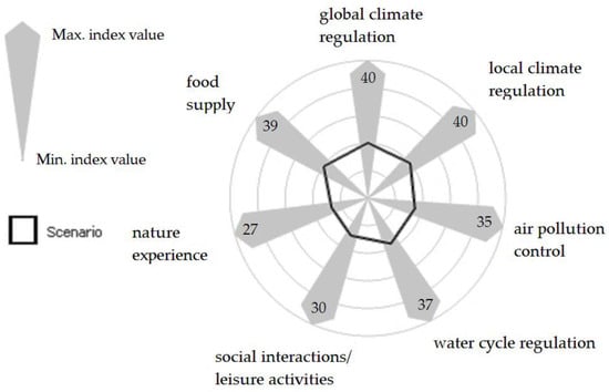
Figure 4.
Spider diagram in GISCAME with average index values for Halle.
3.2.2. Capacity Maps for Regulating Ecosystem Services
The capacity maps for the regulating ES show particularly large deficits for regulating ES in the inner city of Halle, as well as in the eastern district of Freiimfelde (Figure 5). Furthermore, the southern and northern inner city parts have very little potential for the provision of regulating ES. All other urban districts have slightly higher potentials for the provision of regulating ES. The Dölauer Heide in the northwest, the Saale floodplain in the center of the city, and the forest areas in the northeast are rated with high index values.
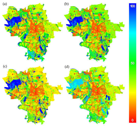
Figure 5.
Capacity maps for the regulatory ecosystem services: (a) global climate regulation, (b) local climate regulation, (c) air pollution control, and (d) water cycle regulation. Value 100 (blue) = highest ecosystem service capacity; 0 (red) = lowest/no ecosystem service capacity.
Capacities for regulating ES provided by natural grassland in particular are assessed very differently in the Burkhard Matrix, depending on the ES considered, so that the Saale–Elster meadow in the south of Halle makes a major contribution to global climate regulation, but has only a low potential for improving air quality. Only slight differences exist between local (Figure 5a) and global climate regulation (Figure 5b). The northern and western parts of Halle are dominated by arable land and therefore have little potential for the provision of regulating ES.
3.2.3. Capacity Maps for the Cultural Ecosystem Services
Two different capacity maps were created for the cultural ES “recreation,” which evaluate the definitions of recreation in the city as described in Section 2.4. Deficits in the provision of recreational facilities are particularly noticeable in the center and eastern parts of the city. Only small and non-networked public recreational areas are accessible for many residents in the immediate vicinity.
The capacity map for recreational performance with a focus on nature experience (Figure 6a) shows that there are no areas for nature experiences with an index value above 50 in the core area of the city. However, the recreational areas close to the city center usually achieve a high index value for the recreational performance “social interaction and leisure activities” (Figure 6b). In general, there is often a certain trade-off between the two recreational services.
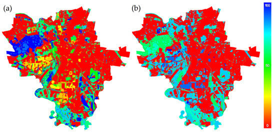
Figure 6.
Capacity map for the recreation service “nature experience” (a) and “social interaction and leisure activities” (b). Value 100 (blue) = highest ecosystem service capacity; 0 (red) = lowest/no ecosystem service capacity.
The forest areas on the banks of the Saale, parts of the Saale–Elster meadow in the south, forest areas in Radewell–Osendorf and the Dölauer Heide are large-scale nature experience areas in the city of Halle and have been evaluated with an index value of over 50. In the northern part of the city of Halle, there are small-scale areas with high index values of nature experience. In addition, in Neustadt in the west of Halle, as well as in the southern part of the city, there are many public green areas and open spaces. This is due to the types of buildings (row development, high-rise buildings) in these districts, which make it possible to use or cross the green spaces of these residential areas (see Section 2.3.3).
3.2.4. Capacity Map for the Provisioning Ecosystem Service “Food Supply”
The capacity map for food supply (Figure 7) shows the highest potential in the peripheral areas of Halle. These are, in particular, arable cropland and commercial horticultures, which are classified as urban agriculture and have an index value of 100. Only a low potential for food supply can be recognized in the southern suburbs of Halle, since protected landscape areas of the Saale–Elster meadow and extensive grassland predominates. Higher potential for the provision of food can be seen in the southern, northern and western parts of the city districts. This is due to the high proportion of allotments, which were valued with the index value 75. An increase in the index value for food supply can also be seen with increasing distance to the city center.
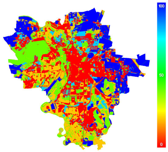
Figure 7.
Capacity map for food supply. Value 100 (blue) = highest ecosystem service capacity; 0 (red) = lowest/no ecosystem service capacity.
4. Discussion
4.1. Ecosystem Services Capacity in Halle
The inner city of Halle has a low capacity for regulatory ES and no capacity for providing cultural ES and food, which could be related to the lack of accessible green open spaces for cultural ES and the absence of agricultural areas for food provision. The finding that the index value of food provision increased with increasing distance to the city center is also supported by Kroll et al. (2012) [62]. They conducted an ES analysis in the Leipzig–Halle region. They presented supply and demand ratios of food, water and energy for 1990, 2000 and 2007 on a rural–urban gradient. They could also identify that the most fertile soils located around Halle were converted to urban areas during this period. Urban growth and increasing biofuel crop cultivation had negative effects on food provision but did not outweigh the net provision of food due to increased productivity per hectare at the same time. Similarly, Bauer et al. (2013) [26] identified in a scenario assessment of ES that food and energy provision would increase even if arable land remained stable in the area. Haase et al. (2012) [55] could identify trade-offs between climate regulation and food provision in the Leipzig-Halle region, among others.
Trees in the inner city are mainly allocated to the courtyards of the quarters and, therefore, are not accessible by the general public (no cultural ES), and tree avenues are rare in Halle. In the peripheral areas of the inner city, provision levels of all ES are higher but scattered. In the southern part of Halle, allotment gardens and the cemetery provide regulating ES. High provisional levels of ES are given for the Dölauer Heide in the north-west of Halle. This forest area is an important ES provider. Lupp et al. (2016) [63] did a ranking with visitors of two urban forests in the Munich Metropolitan region where it was stated that air purification would be the most important ES. The results provided in Baró et al. (2014) [64] for urban forests in Barcelona showed that climate regulation provided by urban forests can contribute substantially to meet the climate policy targets of a city.
In our study, high capacities of multiple ES were also provided by the Saale–Elster floodplain and Saale–Elster meadow. Floodplain areas are also important for flood control [65], but this ES was not assessed in this study. Together with Dölauer Heide, these areas are already protected landscapes. Future planning must ensure the quality of these important ES-providing areas. Furthermore, new ES potentials could emerge in future. Mid-term trends until 2025 show that the population of Halle is stagnating or even decreasing again. A rather poor employment development is predicted [66]. The urban development concept is focusing on dismantling real estates in the fringes of Halle. In addition, Halle would like to strengthen its image as a “green city” [25].
From the perspective of spatial distribution of ES regarding environmental justice, the districts where its inhabitants are more often affected by socio-economic problems (e.g., unemployment, relative poverty), such as Halle–Neustadt and Silberhöhe [25], showed low ES provision levels, but these levels were comparable to other districts without socio-economic problems. In addition, Breuste (2004) [54] could not identify significant differences in the usage (frequency, location) of open spaces in Halle by residents from two districts with different socio-economic backgrounds. However, ES provision is not evenly distributed across the city. ES deficits exist especially for the inner city of Halle where the density of buildings and sealed areas are high. In this case, the greening of cities, e.g., greening roofs [67], green walls/facades [68] and pots and planters could contribute to increase ES capacities of urban centers and compact districts.
4.2. Assessment Approach and Database
The hemeroby concept applied in this work, with the indicators “sealing degree” and “tree cover degree,” enables a stringent classification of BTNT areas and can therefore be used quickly and cost-effectively to inform on the naturalness of urban areas. This approach allows the integration of the detailed information of different vegetation types and quality of urban land use types in the assessment of ES. In order to obtain more precise results, information on the species of trees and shrubs and on the land use of the areas in the built-up areas would be necessary, but these are not included in the BTNT. In addition, the use of the municipal tree cadaster is also suitable, as physiological information and vitality data from city trees can be included in the evaluation. However, it is problematic that only trees owned by the city are included in the database and therefore it is not possible to survey all city trees of Halle. However, by focusing on public space, the integration would lead to a much more precise result. Furthermore, the integration of point and line data from the BTNT would also refine the results, since some tree rows or other succinct vegetation elements are contained as lines or points in the data set. The area classification, which describes the land use and hemeroby, as well as the accessibility of the BTNT areas of Halle, can be used as a functional approach for mapping urban ES and can be used to derive information on the provision of urban ES in various quarters and districts of Halle.
The ES “recreation” was separated into “social interaction and leisure activities” and “experience of nature” in order to acknowledge differences in the provision of cultural ES. The presented approach is suitable for a differentiated examination of recreational services, since the composition of areas with recreational functions influences the type of recreational services. For studies dealing with the collection of urban recreation functions on the basis of distance and buffer analyses [36], the present approach could help to achieve more precise results and to enable the collection of individual aspects of recovery. If, for example, there are only very remote open spaces with recreational functions in the surrounding area, this approach could be used to identify a lack of space for nature experiences in the neighborhood.
Weaknesses in the accuracy of results could not be avoided due to partially generalized approaches and assumptions. For example, the hemeroby classification was relatively broad and contains uncertainties in the determination of ES provision levels. Similarly, the Burkhard Matrix used for devaluation only indicates approximate capacities for the provision of ES for individual biotopes and land use types of a central European standard landscape. In order to achieve more precise results after the devaluation, the evaluation of ES capacities could be carried out in an expert workshop or with other land use information (e.g., [29,69]). For example, capacities for regulating ES could be differentiated more precisely according to the type of land use. In addition, urban land use classes could be used instead of CORINE land cover classes for valuation purposes, so that, for example, allotment gardens are treated as a separate type of use.
The assessment of the accessibility of urban nature was also relatively broad, but it can be seen that housing areas also have some freely accessible green spaces and open spaces, which partly include leisure facilities or playgrounds. This circumstance shows that some housing areas can have recreational functions. The assessment of food supply was relatively imprecise in this work, because hemeroby evaluations and urban land use types carry little significance in the assessment of this ES. The assessment of land use types such as allotments remains a challenge, as harvest volumes and cultivation vary widely.
The set of the regional biotope and land use data was based on 2009 data, which could have caused uncertainty in the results as well. In 2010, the population of Halle was slightly increased after a long period of population decrease [70]. Consequently, vacant houses could be used again, and the housing stock remained constant (2012–2017). Even though there might have been minor structural dynamics, we assume that no significant changes in ES provision levels took place within that period.
In general, participatory workshops, expert consultation or quantitative surveys would have improved the quality of the results (e.g., [71,72]). In particular, questions of environmental justice need to be answered by participatory approaches [73,74]. In addition, the index values for “social interaction and leisure activities” could be ascertained through citizen participation processes, as these represent the most subjective topics. In addition, the assessment of the recreational ES “experience of nature” seems to be more suitable in studies of hemeroby, as it was used in other studies as an indicator for determining the recreational performance [75].
4.3. Impact for Urban Planning and Decision Making
The approach presented in this paper is suitable for comparing the environmental quality and ES capacities of cities, as the BTNT is available for the whole of Saxony–Anhalt. Similar data sets are also available in other federal states on the basis of color-infrared photos, which follow a standardized mapping key, but often use other scales and indicators to map the nature of urban areas. For the comparison of index values, the evaluation possibilities in GISCAME are suitable, in which, among other things, the average index values for certain ES of the investigated regions are displayed and can be compared to other local conditions [76]. For example, if the methodology under study were to be applied to Magdeburg, the provision of ES could be compared against the average index value of the two cities. The GISCAME evaluation function also makes it possible to compare districts or parts of municipal areas and to make useful planning recommendations on a neighborhood scale.
In addition, it could be possible to assess time-related aspects and dynamics which change the provision of ES by means of detecting changes and also visualizing these changes in the spider diagram in GISCAME. Furthermore, trade-offs between ES in different scenarios could be assessed. In a change detection process, differences in Halle’s urban ecosystems and urban ES can be identified by comparing two sets of data from different years [77]. Examples of ES change analyses are shown by Haase et al. (2012) [55] and Kroll et al. (2012) [62] for the study area. Kroll et al. (2012) [62] showed that changes in land use intensity had a more relevant impact on ES supply than changes in land cover for the Leipzig–Halle region. This emphasizes the need for a more differentiated assessment of land use intensities, as our study suggests. The survey of changes in individual ES is also particularly important, as it makes it possible to clarify the effects of interventions, planning and other policy measures [53].
5. Conclusions
Saving and expanding urban open spaces and urban nature is an important social task in times of increasing urbanization. The presented approach can help cities and municipalities to make them more sustainable and environmentally friendly by taking into account ES assessments in planning decisions. In addition to the consideration of the economic costs and benefits of planning measures, arguments for the preservation and expansion of urban nature and urban ecosystems can also be better represented.
On the basis of hemeroby and ES assessment, interested city dwellers could be better informed about different types and services of urban nature and express more precisely through these findings the requirements and needs for public green spaces and open spaces. This can help urban planners to operate citizen-oriented and successful open space planning.
For the city of Halle, which has set itself the goal of further strengthening its green image and expanding green spaces, application of the ES concept and the present approach is also suitable for locating deficits in the provision of ES. Although the proportion of green spaces and recreational areas in the city is high, there are quarters and districts with ES deficits. In particular, the inner city of Halle has a low capacity for regulatory ES and almost no capacity for providing food, nature experiences and leisure activities. Equal provision of green spaces and recreational facilities throughout the city should be the goal of environmentally sound urban planning to ensure quality of life, health and good social relations throughout the city.
Key lessons:
- The assessment approach contributes to the localization and a refined estimation of urban ES provision levels.
- The consideration of hemeroby represents a more differentiated ES assessment adapted to the context of urban areas.
- A sub-classification of ES (in our case, the cultural ES “recreation”) should be taken into account since they might also differ in ES provision.
Author Contributions
This work originated at the Department of Sustainable Landscape Development at Martin-Luther University Halle-Wittenberg. J.A. and C.F. conceived and designed the study. J.A. collected and analyzed the data and performed the literature review. J.A. and J.K. developed and wrote the paper. C.F. reviewed the paper.
Funding
We acknowledge the financial support by the Martin-Luther University Halle-Wittenberg within the funding program for Open Access Publishing by the German Research Foundation (DFG).
Acknowledgments
We would like to thank Paul Ronning for his professional English proofreading of the paper. In addition, we thank Lydia Gorn for her support in formatting the references.
Conflicts of Interest
The authors declare no conflict of interest.
Appendix A. Examples of Building Types and Accessibility of Green Space

Figure A1.
Example of high-rise buildings in Halle Neustadt with public green spaces (Google Maps 2018).
Figure A1.
Example of high-rise buildings in Halle Neustadt with public green spaces (Google Maps 2018).


Figure A2.
Example of old perimeter development/old buildings with private green space (Google Maps 2018).
Figure A2.
Example of old perimeter development/old buildings with private green space (Google Maps 2018).


Figure A3.
Example of modern perimeter development with public green spaces (Google Maps 2018).
Figure A3.
Example of modern perimeter development with public green spaces (Google Maps 2018).

Appendix B. Detailed Description of Selected Ecosystem Services
Appendix B.1. Global Climate Regulation
Urban areas are among the main emitters of greenhouse gas emissions and therefore have a high impact on global climate change [78]. This is particularly due to the high population density in cities and the use of fossil fuels. The fact that urban ecosystems also contribute to global climate regulation in the form of carbon sequestration [42] is important. Carbon from the CO2 in the air is incorporated into plant biomass via photosynthesis, bound in soils and vegetation and released again by decomposition. Generally, more CO2 is stored than released, so that a contribution to climate protection is made. However, due to the high emissions of greenhouse gases in cities, only a small part of the emissions from urban ecosystems can be compensated [43]. This is illustrated in a study in Lübeck in which residential, commercial and traffic areas released 296.7 tons of CO2 equivalent per year, while adjacent forest and forest-like areas could only bind 8.5 tons of CO2 equivalent per hectare per year [79]. Carbon is mainly stored by trees and other long-lived vegetation elements. The total amount of storage depends on the age and size of the urban trees [80]. Furthermore, peatlands, peat bogs and natural grasslands store large amounts of carbon and have high capacities for the global climate regulation ecosystem service [31].
Appendix B.2. Local Climate Regulation
The high proportion of sealed areas and dense cultivation change the urban climate, the weather conditions and the heat balance compared to the rural areas. By draining rainwater via sewer systems, less water is stored in the soil, and evaporation is up to 50% lower than in non-built-up areas [81]. Likewise, plant evaporation (transpiration) is reduced by the low proportion of vegetation and the high rates of sedimentation [82]. As a result, only a small portion of the solar radiant energy is used for evapotranspiration, and is instead stored in roofs, walls, and sealed areas. At night, the radiation energy is released back to the ground-level air and prevents cooling of the built-up and sealed surfaces so that “urban heat islands” arise. In addition, anthropogenic processes like combustion and energy conversion in industry and traffic contributes to heat generation in urban areas [37]. In serene weather conditions, heat islands develop in cities which can result in nighttime temperature differences of up to 10 degrees Celsius compared to the rural areas in the region. This effect is further intensified by heat waves in the summer, as well as climate change, so that urban heat stress is already leading to increased mortality [82].
Urban vegetation regulates the urban climate by intercepting solar radiation (shading), by the process of evapotranspiration and by changing the air movement and heat exchange. Shading and evapotranspiration contribute the most to a cooling effect [41]. The cooling effect of urban nature is one to four degrees Celsius and depends on the surface and vegetation type [44]. Urban green spaces can lower the higher temperatures in surrounding areas if the building structure and topographical conditions permit air flow [45].
Appendix B.3. Air Pollution Control
Cities have low levels of aeration in relation to rural areas. As a result, gaseous as well as particulate pollutants caused by industry, transport, waste treatment and heating reduce the air quality. The result is a negative impact on the health of inhabitants [46]. In particular, the frequency of cardiovascular and respiratory diseases is increased by the poor air quality [83].
Urban vegetation filters contaminant particles, such as nitrogen dioxide (NO2), through deposition, sedimentation, diffusion, turbulence or leaching [37]. In addition, oxygenation from urban vegetation is an important factor in improving air quality [46].
Appendix B.4. Water Cycle Regulation
Due to the high proportion of sealed surfaces and canalization, natural drainage in cities is hampered. The higher the degree of soil sealing, the higher the direct runoff of rain water. As a result, increased peak flows in cities leads to more frequent and severe local floods [84]. Furthermore, high sealing reduces the effective leach rate and decreases real evapotranspiration, which further enhances the effects of flooding [85].
Urban nature diminishes the effects described above by intercepting precipitation, storing water or infiltrating water into soil. In particular, trees and shrubs catch precipitation and release it into the atmosphere via evaporation, while grassland absorbs water by infiltration [47].
Appendix B.5. Nature Experience and Social Interactions/Leisure Activities
According to Grunewald and Bastian (2013) [53], the ecosystem service “opportunities for recreation and (eco-) tourism” is defined by the “possibility of practicing sports, leisure and recreational activities in nature and landscape.” The recreation services in urban areas are of particular importance [86], as the need for places to rest, compared to rural areas, are very high [31]. Recent research indicates that the physical and mental health of city dwellers is increased by staying in green spaces [37]. Furthermore, the quality of life of the neighborhood is increased by green spaces and the attractiveness of cities improves with good provision of green areas [37]. Recreational performance is a cultural ecosystem service that is closely linked to aesthetics, so that scenic beauty enhances the recreational potential of the area [50]. Most parks, public gardens and similar intensively designed and maintained places are at the center of the general interest, because they offer individual opportunities for leisure, sport and social activities. In addition, they have high aesthetic value [40].
However, very natural green areas, which offer space for nature experiences, play an important role in the urban context and are therefore described and evaluated individually in this work.
According to Bögeholz (1999) [87], the natural experience is differentiated into four different types:
- Aesthetic nature experience: sensual experience of beauty and uniqueness of nature
- Exploring nature experience: examining animals and plants
- Instrumental nature experience: maintaining and use of animals and plants
- Social nature experience: building a relationship with animals, plants and natural places
Spaces for experiencing nature and tranquility are rare in cities and receive little attention, but in times of an urbanized and digitized society, they are of elementary importance. Of particular concern is the fact that awareness of nature continues to decline among young people [88].
Children and young people are helped by nature experiences in the development and training of motor, mental and social skills [49]. Nature experiences close to residential areas offer a suitable opportunity for this and must be protected or expanded, because only if children have the opportunity to experience nature, they can build a relationship to nature [87]. Nature experience spaces are not only of major importance for young people and children. Regular contact with nature promotes health and enhances human well-being [48].
Nature experience spaces are largely undeveloped living spaces left to their natural development, in contrast to intensively maintained and designed parks and gardens. In addition, designed parks can also be equipped with diverse natural components such as old trees, flowing and still waters, and near-natural meadows which contribute to the natural experience of the inhabitants [40]. In surveys by Riechers et al. in 2015 [89], it became apparent that the experience of nature is one of the most important criteria of respondents for the design of open and green spaces.
In contrast to the assessment of regulatory ecosystem services, even non-natural parks can have a high potential to provide recreation services, as they are characterized by open vegetation structures and offer a lot of space, equipment and structures for social interaction and leisure activities. Therefore, it makes sense to assess two different forms of recreation individually: on the one hand, a recreation service which describes the potential for rest and nature experiences and on the other hand, a recreation service which describes the potential for social interaction and leisure activities.
To assess the recreation services, the hemeroby classification, biotope and land use type classification as well as the public accessibility of the area are included. In this way, all areas that are not publicly accessible are evaluated with the index value 0.
Appendix B.6. Food Supply
Food production in urban areas has been increasingly pursued in research and by the public for several years. The generic term “urban agriculture” is usually subdivided into two different areas. On the one hand is “urban agriculture,” which is market-oriented, specialized and characterized by professionalism [51]. On the other hand, “urban gardening” represents a civic and subsistence-oriented agriculture [90].
Gardening in urban areas is an important part of urban life, as it not only provides food, but also space for other cultural ecosystem services such as recreation, social relations and environmental education [91]. Examples of urban gardening are urban gardening projects, such as the Prinzessinnengarten in Berlin, but also allotment gardens, which play an above-average role in the city of Halle (Saale) compared to other major German cities. In addition to urban agriculture, other biotopes of urban nature provide food, such as blackberries, mushrooms, wild herbs or fruit.
References
- Birch, E.; Wachter, S. World urbanization: The critical issue of the twenty-first century. In Global Urbanization; University of Pennsylvania Press: Philadelphia, PA, USA, 2011; pp. 3–23. [Google Scholar]
- United Nations. World Urbanisation Prospects: The 2018 Revision. Key Facts. Economic and Social Affairs; United Nations: New York, NY, USA, 2018. [Google Scholar]
- Gómez-Baggethun, E.; Barton, D.N. Classifying and valuing ecosystem services for urban planning. Ecol. Econ. 2013, 86, 235–245. [Google Scholar] [CrossRef]
- De Groot, R.S.; Wilson, M.A.; Boumans, R.M.J. A typology for the classification, description and valuation of ecosystem functions, goods and services. Ecol. Econ. 2002, 41, 393–408. [Google Scholar] [CrossRef]
- Daily, G.C.; Polasky, S.; Goldstein, J.; Kareiva, P.M.; Mooney, H.A.; Pejchar, L.; Ricketts, T.H.; Salzman, J.; Shallenberger, R. Ecosystem services in decision making: Time to deliver. Front. Ecol. Environ. 2009, 7, 21–28. [Google Scholar] [CrossRef]
- Haines-Young, R.; Potschin, M. The links between biodiversity, ecosystem services and human well-being. In Ecosystem Ecology: A New Synthesis; Raffaelli, D., Frid, C., Eds.; Cambridge University Press: Cambridge, UK, 2010; pp. 110–139. [Google Scholar]
- TEEB. The Economics of Ecosystems and Biodiversity: Mainstreaming the Economics of Nature: A Synthesis of the Approach, Conclusions and Recommendations of TEEB; TEEB: Geneva, Switzerland, 2010. [Google Scholar]
- Díaz, S.; Demissew, S.; Carabias, J.; Joly, C.; Lonsdale, M.; Ash, N.; Larigauderie, A.; Adhikari, J.R.; Arico, S.; Báldi, A.; et al. The IPBES Conceptual Framework—Connecting nature and people. Curr. Opin. Environ. Sustain. 2015, 14, 1–16. [Google Scholar] [CrossRef]
- Haines-Young, R.; Potschin, M. Proposal for a Common International Classification of Ecosystem Goods and Services (CICES) for Integrated Environmental and Economic Accounting; European Environment Agency: Copenhagen, Denmark, 2010; Volume 30. [Google Scholar]
- Stadtökosysteme. Funktion, Management und Entwicklung, 1st ed.; Breuste, J., Pauleit, S., Haase, D., Sauerwein, M., Eds.; Springer Spektrum: Berlin/Heidelberg, Germany, 2016. [Google Scholar]
- Ishii, M. Measurement of road traffic noise reduced by the employment of low physical barriers and potted vegetation. Inter-Noise Noise-Con Congr. Conf. Proc. 1994, 29–31, 595–598. [Google Scholar]
- Nowak, D.J.; Hirabayashi, S.; Bodine, A.; Greenfield, E. Tree and forest effects on air quality and human health in the United States. Environ. Pollut. 2014, 193, 119–129. [Google Scholar] [CrossRef] [PubMed]
- Andersson, E.; Barthel, S.; Borgström, S.; Colding, J.; Elmqvist, T.; Folke, C.; Gren, Å. Reconnecting cities to the biosphere: Stewardship of green infrastructure and urban ecosystem services. Ambio 2014, 43, 445–453. [Google Scholar] [CrossRef] [PubMed]
- Hope, D.; Gries, C.; Zhu, W.; Fagan, W.F.; Redman, C.L.; Grimm, N.B.; Nelson, A.; Martin, C.; Kinzig, A. Socio-economics drive urban plant diversity. Proc. Natl. Acad. Sci. USA 2003, 100, 8788–8792. [Google Scholar] [CrossRef] [PubMed]
- Graves, R.A.; Pearson, S.M.; Turner, M.G. Landscape dynamics of floral resources affect the supply of a biodiversity-dependent cultural ecosystem service. Landsc. Ecol. 2017, 32, 415–428. [Google Scholar] [CrossRef]
- Aronson, M.F.J.; Lepczyk, C.A.; Evans, K.L.; Goddard, M.A.; Lerman, S.B.; MacIvor, J.S.; Nilon, C.H.; Vargo, T. Biodiversity in the city: Key challenges for urban green space management. Front. Ecol. Environ. 2017, 15, 189–196. [Google Scholar] [CrossRef]
- Ziter, C. The biodiversity-ecosystem service relationship in urban areas: A quantitative review. Oikos 2016, 125, 761–768. [Google Scholar] [CrossRef]
- Bastian, O.; Haase, D.; Grunewald, K. Ecosystem properties, potentials and services—The EPPS conceptual framework and an urban application example. Ecol. Indic. 2012, 21, 7–16. [Google Scholar] [CrossRef]
- Wolch, J.R.; Byrne, J.; Newell, J.P. Urban green space, public health, and environmental justice: The challenge of making cities ‘just green enough’. Landsc. Urban Plan. 2014, 125, 234–244. [Google Scholar] [CrossRef]
- Jalas, J. Hemerobe and hemerochore Pflanzenarten: Ein terminologischer Reformversuch. Acta Soc. Pro Fauna Flora Fenn. 1955, 72, 1–15. [Google Scholar]
- Sukopp, H. Wandel von Flora und Vegetation in Mitteleuropa unter dem Einfluß des Menschen. Berichte Landwirtsch. 1972, 50, 112–139. [Google Scholar]
- Schumacher, U.; Lehmann, I.; Behnisch, M. Modellansatz zur geotopographischen Analyse von Wohngebieten und urbaner grüner Infrastruktur. AGIT J. Angew. Geoinform. 2016, 2, 540–545. [Google Scholar] [CrossRef]
- Beichler, S.A.; Bastian, O.; Haase, D.; Heiland, S.; Kabisch, N.; Müller, F. Does the Ecosystem Service Concept Reach its Limits in Urban Environments? Landsc. Online 2017, 51. [Google Scholar] [CrossRef]
- Pauleit, S.; Duhme, F. Assessing the environmental performance of land cover types for urban planning. Landsc. Urban Plann. 2000, 52, 1–20. [Google Scholar] [CrossRef]
- Stadt Halle (Saale). ISEK Halle Saale 2025; Stadt Halle: Halle, Germany, 2016. [Google Scholar]
- Bauer, A.; Röhl, D.; Haase, D.; Schwarz, N. Leipzig-Halle: Ecosystem Services in a Stagnating Urban Region in Eastern Germany. In Peri-Urban Futures: Scenarios and Models for Land Use Change in Europe; Nilsson, K., Ed.; Springer: Berlin/Heidelberg, Germany, 2013; pp. 209–239. [Google Scholar]
- Bundesamt für Kartographie und Geodäsie. ©GeoBasis-DE/BKG; BKG: Frankfurt, Germany, 2018.
- Fürst, C.; Volk, M.; Pietzsch, K.; Makeschin, F. Pimp your landscape: A tool for qualitative evaluation of the effects of regional planning measures on ecosystem services. Environ. Manag. 2010, 46, 953–968. [Google Scholar] [CrossRef] [PubMed]
- Koschke, L.; Fürst, C.; Frank, S.; Makeschin, F. A multi-criteria approach for an integrated land-cover-based assessment of ecosystem services provision to support landscape planning. Ecol. Indic. 2012, 21, 54–66. [Google Scholar] [CrossRef]
- Giscame. 2018. Available online: https://www.giscame.com/giscame/english_home.html (accessed on 6 July 2018).
- Burkhard, B.; Kandziora, M.; Hou, Y.; Müller, F. Ecosystem Service Potentials, Flows and Demands-Concepts for Spatial Localisation, Indication and Quantification. Landsc. Online 2014, 34, 1–32. [Google Scholar] [CrossRef]
- Walz, U.; Stein, C. Indicators of hemeroby for the monitoring of landscapes in Germany. J. Nat. Conserv. 2014, 22, 279–289. [Google Scholar] [CrossRef]
- Blume, H.-P.; Sukopp, H. Ökologische Bedeutung anthropogener Bodenveränderungen. Schriftenreihe Vegetationskunde 1976, 10, 75–89. [Google Scholar]
- Schlüter, H. Natürlichkeitsgrad der Vegetation. In Analyse und Ökologische Bewertung der Landschaft, 2nd ed.; Bastian, O., Schreiber, K.-F., Eds.; Spektrum Akademischer Verlag: Heidelberg/Berlin, Germany, 1999. [Google Scholar]
- Landesamt für Umweltschutz Sachsen-Anhalt. Katalog der Biotoptypen und Nutzungstypen für die CIR-luftbildgestützte Biotoptypenkartierung im Land Sachsen-Anhalt. In Berichte des Landesamtes für Umweltschutz Sachsen-Anhalt; Landesamtes für Umweltschutz Sachsen-Anhalt: Halle (Saale), Germany, 1992. [Google Scholar]
- Grunewald, K.; Richter, B.; Meinel, G.; Herold, H.; Syrbe, R.-U. Proposal of indicators regarding the provision and accessibility of green spaces for assessing the ecosystem service “recreation in the city” in Germany. Int. J. Biodivers. Sci. Ecosyst. Serv. Manag. 2017, 13, 26–39. [Google Scholar] [CrossRef]
- Haase, D. Was leisten Stadtökosysteme für die Menschen in der Stadt? In Stadtökosysteme: Funktion, Management und Entwicklung, 1st ed.; Breuste, J., Pauleit, S., Haase, D., Sauerwein, M., Eds.; Springer Spektrum: Berlin/Heidelberg, Germany, 2016; pp. 129–163. [Google Scholar]
- Bundesministerium für Umwelt. Naturschutz, Bau und Reaktorsicherheit. In Grün in der Stadt—Für Eine Lebenswerte; Zukunft: Berlin, Germany, 2015. [Google Scholar]
- Haase, A.; Eichhorn, S. Öffentliche und Private Räume—Gebaute und Gelebte Räume; Jahrbuch der Stadterneuerung: Berlin, Germany, 2004; pp. 359–376. [Google Scholar]
- Knapp, S.; Keil, A.; Keil, P.; Reidl, K.; Rink, D.; Schemel, H.J. Naturerleben, Naturerfahrung und Umweltbildung in der Stadt. In Naturkapital Deutschland TEEB (2016): Ökosystemleistungen in der Stadt. Gesundheit Schützen und Lebensqualität Erhöhen; TU Berlin, Helmholtz-Zentrum für Umweltforschung UFZ Berlin: Leipzig, Germany, 2016; pp. 146–169. [Google Scholar]
- Skelhorn, C.; Lindley, S.; Levermore, G. The impact of vegetation types on air and surface temperatures in a temperate city: A fine scale assessment in Manchester, UK. Landsc. Urban Plan. 2014, 121, 129–140. [Google Scholar] [CrossRef]
- Strohbach, M.W.; Haase, D. Above-ground carbon storage by urban trees in Leipzig, Germany: Analysis of patterns in a European city. Landsc. Urban Plan. 2012, 104, 95–104. [Google Scholar] [CrossRef]
- Pataki, D.E.; Alig, R.J.; Fung, A.S.; Golubiewski, N.E.; Kennedy, C.A.; McPherson, E.G.; Nowak, D.J.; Pouyat, R.V.; Romero Lankao, P. Urban ecosystems and the North American carbon cycle. Glob. Chang. Biol. 2006, 12, 2092–2102. [Google Scholar] [CrossRef]
- Xie, M.; Wang, Y.; Chang, Q.; Fu, M.; Ye, M. Assessment of landscape patterns affecting land surface temperature in different biophysical gradients in Shenzhen, China. Urban Ecosyst. 2013, 16, 871–886. [Google Scholar] [CrossRef]
- Gill, S.E.; Handley, J.F.; Ennos, A.R.; Pauleit, S. Adapting Cities for Climate Change: The Role of the Green Infrastructure. Built Environ. 2007, 33, 115–133. [Google Scholar] [CrossRef]
- Säumel, I.; Draheim, T.; Endlicher, W.; Langner, M. Stadtnatur fördert saubere Luft. In Naturkapital Deutschland TEEB (2016): Ökosystemleistungen in der Stadt. Gesundheit Schützen und Lebensqualität Erhöhen; TU Berlin, Helmholtz-Zentrum für Umweltforschung UFZ Berlin: Leipzig, Germany, 2016. [Google Scholar]
- Armson, D.; Stringer, P.; Ennos, A.R. The effect of street trees and amenity grass on urban surface water runoff in Manchester, UK. Urban For. Urban Green. 2013, 12, 282–286. [Google Scholar] [CrossRef]
- Maller, C.; Townsend, M.; Pryor, A.; Brown, P.; St Leger, L. Healthy nature healthy people: ‘contact with nature’ as an upstream health promotion intervention for populations. Health Promot. Int. 2006, 21, 45–54. [Google Scholar] [CrossRef] [PubMed]
- Kellert, S.R. Experiencing nature: Affective, cognitive, and evaluative development in children. In Children and Nature: Psychological, Sociocultural, and Evolutionary Investigations; MIT Press: Cambridge, MA, USA, 2002. [Google Scholar]
- Derkzen, M.; van Teeffelen, A.J.A.; Verburg, P.H.; Diamond, S. Quantifying urban ecosystem services based on high-resolution data of urban green space: An assessment for Rotterdam, The Netherlands. J. Appl. Ecol. 2015, 52, 1020–1032. [Google Scholar] [CrossRef]
- Born, R.; Pölling, B. Urbane Landwirtschaft in der Metropole Ruhr. B&B Agrar 2014, 2, 9–12. [Google Scholar]
- Galluzzi, G.; Eyzaguirre, P.; Negri, V. Home gardens: Neglected hotspots of agro-biodiversity and cultural diversity. Biodivers. Conserv. 2010, 19, 3635–3654. [Google Scholar] [CrossRef]
- Grunewald, K.; Bastian, O. Ökosystemdienstleistungen. Konzept, Methoden und Fallbeispiele; Springer Spektrum: Heidelberg, Germany, 2013. [Google Scholar]
- Breuste, J.H. Decision making, planning and design for the conservation of indigenous vegetation within urban development. Landsc. Urban Plan. 2004, 68, 439–452. [Google Scholar] [CrossRef]
- Haase, D.; Schwarz, N.; Strohbach, M.; Kroll, F.; Seppelt, R. Synergies, trade-offs, and losses of ecosystem services in urban regions: An integrated multiscale framework applied to the Leipzig-Halle Region, Germany. Ecol. Soc. 2012, 17, 22. [Google Scholar] [CrossRef]
- Stein, C.; Walz, U. Hemerobie als Indikator für das Flächenmonitoring. Methodenentwicklung Beispiel von Sachsen/Hemeroby as Indicator for the Monitoring of Land Use—Development of methods using the example of Saxony. Naturschutz Landschaftsplanung 2012, 44, 261–266. [Google Scholar]
- García-Llorente, M.; Martín-López, B.; Iniesta-Arandia, I.; López-Santiago, C.A.; Aguilera, P.A.; Montes, C. The role of multi-functionality in social preferences toward semi-arid rural landscapes: An ecosystem service approach. Environ. Sci. Policy 2012, 19–20, 136–146. [Google Scholar] [CrossRef]
- Stadt Halle (Saale). Erlass Einer Satzung zum Schutze des Stadtwaldes “Dölauer Heide”. 1954. Available online: http://www.halle.de/Publications/4520/sr925.pdf (accessed on 6 February 2018).
- Stadt Halle (Saale). Verordnung zur Festsetzung des Naturschutzgebietes “Forstwerder”. 1998. Available online: http://www.halle.de/Publications/3264/nsg_forstwerder.pdf (accessed on 6 February 2018).
- Breuste, J.H.; Artmann, M. Allotment Gardens Contribute to Urban Ecosystem Service: Case Study Salzburg, Austria. J. Urban Plan. Dev. 2015, 141, A5014005. [Google Scholar] [CrossRef]
- Stadt Halle (Saale). Kleingartenkonzeption Halle (Saale); Stadt Halle: Halle, Germany, 2012. [Google Scholar]
- Kroll, F.; Müller, F.; Haase, D.; Fohrer, N. Rural–urban gradient analysis of ecosystem services supply and demand dynamics. Land Use Policy 2012, 29, 521–535. [Google Scholar] [CrossRef]
- Lupp, G.; Förster, B.; Kantelberg, V.; Markmann, T.; Naumann, J.; Honert, C.; Koch, M.; Pauleit, S. Assessing the Recreation Value of Urban Woodland Using the Ecosystem Service Approach in Two Forests in the Munich Metropolitan Region. Sustainability 2016, 8, 1156. [Google Scholar] [CrossRef]
- Baró, F.; Palomo, I.; Zulian, G.; Vizcaino, P.; Haase, D.; Gómez-Baggethun, E. Mapping ecosystem service capacity, flow and demand for landscape and urban planning: A case study in the Barcelona metropolitan region. Land Use Policy 2016, 57, 405–417. [Google Scholar] [CrossRef]
- Jha, A.K.; Bloch, R.; Lamond, J. Cities and Flooding: A Guide to Integrated Urban Flood Risk Management for the 21st Century; The World Bank: Washington, DC, USA, 2012. [Google Scholar]
- Fritzsche, B.; Fuchs, M.; Orth, A.K. Strukturbericht Sachsen-Anhalt; ECONSTOR: IAB-Regional, IAB Sachsen-Anhalt-Thüringen, No. 03/2016; Institut für Arbeitsmarkt- und Berufsforschung (IAB): Nürnberg, Germany, 2016. [Google Scholar]
- Santamouris, M. Cooling the cities—A review of reflective and green roof mitigation technologies to fight heat island and improve comfort in urban environments. Sol. Energy 2014, 103, 682–703. [Google Scholar] [CrossRef]
- Köhler, M. Green facades—A view back and some visions. Urban Ecosyst. 2008, 11, 423–436. [Google Scholar] [CrossRef]
- Frank, S.; Fürst, C.; Koschke, L.; Witt, A.; Makeschin, F. Assessment of landscape aesthetics—Validation of a landscape metrics-based assessment by visual estimation of the scenic beauty. Ecol. Indic. 2013, 32, 222–231. [Google Scholar] [CrossRef]
- Stadt Halle (Saale). Wohnungspolitisches Konzept 2018; Stadt Halle: Halle, Germany, 2018. [Google Scholar]
- Fagerholm, N.; Käyhkö, N.; Ndumbaro, F.; Khamis, M. Community stakeholders’ knowledge in landscape assessments—Mapping indicators for landscape services. Ecol. Indic. 2012, 18, 421–433. [Google Scholar] [CrossRef]
- Kabisch, N. Ecosystem service implementation and governance challenges in urban green space planning—The case of Berlin, Germany. Land Use Policy 2015, 42, 557–567. [Google Scholar] [CrossRef]
- Ahern, J.; Cilliers, S.; Niemelä, J. The concept of ecosystem services in adaptive urban planning and design: A framework for supporting innovation. Landsc. Urban Plan. 2014, 125, 254–259. [Google Scholar] [CrossRef]
- Shi, L.; Chu, E.; Anguelovski, I.; Aylett, A.; Debats, J.; Goh, K.; Schenk, T.; Seto, K.C.; Dodman, D.; Roberts, D.; et al. Roadmap towards justice in urban climate adaptation research. Nat. Clim. Chang. 2016, 6, 131–137. [Google Scholar] [CrossRef]
- Früh-Müller, A.; Hotes, S.; Breuer, L.; Wolters, V.; Koellner, T. Regional Patterns of Ecosystem Services in Cultural Landscapes. Land 2016, 5, 17. [Google Scholar] [CrossRef]
- Frank, S.; Fürst, C.; Witt, A.; Koschke, L.; Makeschin, F. Making use of the ecosystem services concept in regional planning—trade-offs from reducing water erosion. Landsc. Ecol. 2014, 29, 1377–1391. [Google Scholar] [CrossRef]
- Kandziora, M.; Dörnhöfer, K.; Oppelt, N.; Müller, F. Detecting Land Use And Land Cover Changes in Northern German Agricultural Landscapes to Assess Ecosystem Service Dynamics. Landsc. Online 2014, 35, 1–24. [Google Scholar] [CrossRef]
- Revi, A.; Satterthwaite, D.; Aragón-Durand, F.; Corfee-Morlot, J.; Kiunsi, R.B.R.; Pelling, M.; Roberts, D.; Solecki, W. Urban areas. In Climate Change 2014: Impacts, Adaptation, and Vulnerability. Contribution of Working Group II to the Fifth Assessment Report of the Intergovern Mental Panel on Climate Change; Field, C.B., Barros, V.R., Dokken, D.J., Mach, K.J., Mastrandrea, M.D., Bilir, T.E., Chatterjee, M., Ebi, K.L., Estrada, Y.O., Genova, R.C., Eds.; Cambridge University Press: Cambridge, NY, USA, 2014; pp. 535–561. [Google Scholar]
- Hansestadt Lübeck. Thematischer Landschaftsplan. Klimawandel in Lübeck. Vorsorge- und Anpassungsmaßnahmen für die Landnutzungen; Schriftenreihe Deutschen Rates Landespflege: Meckenheim, Germany, 2013; p. 32. [Google Scholar]
- Strohbach, M.V. Stadtnatur fördert Klimaschutz. In Naturkapital Deutschland TEEB (2016): Ökosystemleistungen in der Stadt. Gesundheit Schützen und Lebensqualität Erhöhen; TU Berlin, Helmholtz-Zentrum für Umweltforschung UFZ Berlin: Leipzig, Germany, 2016. [Google Scholar]
- Kuttler, W. Klimatologie, 2nd ed.; UTB Schöningh: Paderborn, Germany, 2013. [Google Scholar]
- Endlicher, W.; Scherer, D.; Büter, B.; Kuttler, W.; Mathey, J.; Schneider, C. Stadtnatur fördert gutes Stadtklima. In Naturkapital Deutschland TEEB (2016): Ökosystemleistungen in der Stadt. Gesundheit Schützen und Lebensqualität Erhöhen; TU Berlin, Helmholtz-Zentrum für Umweltforschung UFZ Berlin: Leipzig, Germany, 2016. [Google Scholar]
- Leiva, G.M.A.; Santibañez, D.A.; Ibarra, E.S.; Matus, C.P.; Seguel, R. A five-year study of particulate matter (PM2.5) and cerebrovascular diseases. Environ. Pollut. 2013, 181, 1–6. [Google Scholar] [CrossRef] [PubMed]
- Sommer, T.; Karpf, C.; Ettrich, N.; Haase, D.; Weichel, T.; Peetz, J.-V.; Steckel, B.; Eulitz, K.; Ullrich, K. Coupled modelling of subsurface water flux for an integrated flood risk management. Nat. Hazards Earth Syst. Sci. 2009, 9, 1277–1290. [Google Scholar] [CrossRef]
- Haase, D. Effects of urbanisation on the water balance—A long-term trajectory. Environ. Impact Assess. Rev. 2009, 29, 211–219. [Google Scholar] [CrossRef]
- Breuste, J.; Haase, D.; Elmqvist, T. Urban landscapes and ecosystem services. In Ecosystem Services in Agricultural and Urban Landscapes; John Wiley & Sons: Hoboken, NJ, USA, 2013; pp. 83–104. [Google Scholar]
- Bögeholz, S. Qualitäten Primärer Naturerfahrung und Ihr Zusammenhang mit Umweltwissen und Umwelthandeln; Springer: Berlin, Germany, 1999. [Google Scholar]
- Naturbewusstsein 2013. Bevölkerungsumfrage zu Natur und biologischer Vielfalt; Bundesministerium für Umwelt, Naturschutz und Reaktorsicherheit, Bundesministerium für Naturschutz, Eds.; BMUB; BfN: Berlin/Bonn, Germany, 2014.
- Riechers, M.; Barkmann, J.; Tscharntke, T. Bewertung Kultureller Ökosystemleistungen von Berliner Stadtgrün Entlang Eines Urbanen-Periurbanen Gradienten; Diskussionspapiere No. 1507; PUBLISSO: Göttingen, Germany, 2015. [Google Scholar]
- Lohrberg, F.; Timpe, A. Urbane Agrikultur–Neue Formen der Primärproduktion in der Stadt. Planerin 2011, 5, 35–37. [Google Scholar]
- Brenck, M.; Hansjürgens, B.; Haase, D.; Hartje, V.; Kabisch, N.; Ring, I.; Born, W. Ansätze zur Erfassung und Bewertung städtischer Ökosystemleistungen. In Naturkapital Deutschland TEEB (2016): Ökosystemleistungen in der Stadt. Gesundheit Schützen und Lebensqualität Erhöhen; TU Berlin, Helmholtz-Zentrum für Umweltforschung UFZ Berlin: Leipzig, Germany, 2016. [Google Scholar]


© 2018 by the authors. Licensee MDPI, Basel, Switzerland. This article is an open access article distributed under the terms and conditions of the Creative Commons Attribution (CC BY) license (http://creativecommons.org/licenses/by/4.0/).