Coupling Characteristics of Ecological Cost, Ecological Value, and Network Ecological Efficiency Across Production–Living–Ecological Space Land-Use Transition Pathways in a Peri-Urban Transition Zone: A Case Study of Wenjiang District, Chengdu, China

Abstract

Peri-urban transition zones experience intense conflicts among production, living, and ecological functions, yet the ecological effects of specific land-use transition pathways remain insufficiently quantified. Most studies of production–living–ecological space (PLES) use land-use transition matrices to quantify aggregate transitions among land-use classes, which limits the identification of coupling relationships and differences among specific pathways across ecological cost (EC), ecological value (EV), and network ecological efficiency (NEE). Using Wenjiang District, Chengdu, as a case study, this study integrates complex network analysis, a coupling coordination model, and CA–Markov scenario simulation to develop a pathway coupling framework. The framework quantifies the coupling of EC, EV, and NEE among eight PLES functional land-use classes from 2000 to 2025, and compares their potential ecological effects under three scenarios from 2030 to 2050. The conversion of agricultural production land to urban living land (APL→ULL) was the dominant pathway, with a net transition area of 28.26 km². The eco-environmental quality index declined from 0.228 to 0.200, a cumulative decrease of 12.3%, and the ecological contribution rate remained negative in every period. Coupling coordination varied markedly among pathways. APL→ULL showed severe imbalance ($D$ = 0.191), APL→CPL showed moderate relative coordination ($D$ = 0.741), and APL→FEL and related restoration pathways showed good relative coordination ($D$ = 0.870 to 0.968). Here, $D$ represents the relative coordination of direction-aligned and normalized indicators within the pathway sample rather than absolute ecological performance. Backcasting yielded a Kappa coefficient of 0.82. The future scenarios indicated that ecological protection could slow but not fully reverse the projected degradation trend. Based on ecological effects, relative coordination, and scenario responses, the major pathways were classified as priority-control, priority-incentive, or conditional-management pathways. By using individual land-use transition pathways as a common unit of analysis, the framework links network structure identification, joint assessment of EC, EV, and NEE, comparison of scenario responses, and management classification. It thereby extends PLES eco-environmental assessment from aggregate area change or single indicators to pathway-level diagnosis and decision support.

1. Introduction

Land-use and land-cover change (LUCC) has become a major driver of regional eco-environmental change under continuing industrialization and urbanization. Its effects include changes in ecosystem service provision, landscape patterns, and eco-environmental quality, and they vary with development stage, land-use structure, and ecological governance [1,2,3,4,5]. As ecological civilization initiatives and territorial spatial planning advance, analyses based only on land classes or area changes are no longer sufficient to address the need to coordinate economic development, spatial expansion, and ecological protection [6]. The production–living–ecological space (PLES) framework classifies land into production, living, and ecological spaces according to its dominant function, providing a functional perspective for examining changes in human–land relationships and their eco-environmental effects [7,8]. Peri-urban transition zones of megacities lie at the interface between built-up areas and surrounding rural areas. They experience simultaneous pressures from construction expansion, agricultural land contraction, and ecological protection, and transitions among spatial functions occur more frequently [9,10,11,12]. Clarifying the ecological effects of individual land-use transition pathways can improve understanding of changes in eco-environmental quality and support pathway-specific spatial management in these areas. However, previous studies have not fully explained how these pathways differ in ecological cost, ecological value, and efficiency in peri-urban transition zones.

Research on the eco-environmental effects of LUCC has gradually developed from aggregate assessment and identification of transition processes to analysis of relationships among multiple indicators and simulation of future scenarios. The eco-environmental quality index (EQI) and the ecological contribution rate (ECR) are mainly used to describe regional aggregate effects associated with changes in the land-use structure [13,14,15,16]. Land-use transition matrices record the direction and magnitude of conversions among land classes. Complex network analysis builds on this information by representing land classes as nodes and conversions as directed edges, allowing the topology, critical nodes, and major pathways of the transition network to be examined [17,18,19,20]. For the quantification of ecological effects, ecological cost (EC) and ecological value (EV) describe the ecological resistance and changes in ecosystem service value associated with land-use transitions, respectively [21,22,23]. Ecological efficiency has different meanings across research fields. In traditional ecology, ecological efficiency generally refers to the proportion of energy or production transferred between adjacent trophic levels [24]. In human-managed systems, eco-efficiency commonly measures value creation relative to resource use or environmental impacts [25]. In complex network research, network efficiency evaluates the ability of a network to transmit information or effects along paths between nodes [26]. Xu et al. [27] further incorporated ecological cost and ecological value into a land-use transition network and proposed network ecological efficiency (NEE) to assess the relative ability of a land ecological network to attain greater ecological value at lower ecological cost. This indicator differs from energy transfer efficiency between trophic levels in both its analytical object and definition, and serves as a functional metric for land-use transition networks. Coupling coordination models further assess the relative coordination among multiple indicators [28,29]. For future land-use change, CA–Markov models combine projections of land-use quantities with neighborhood-based spatial allocation and can compare potential land-use patterns under different development constraints [30,31,32,33]. Together, these approaches provide complementary information on aggregate effects, transition structure, relationships among indicators, and future scenarios, which supports an integrated analysis.

Despite these advances, four related limitations remain. First, many studies infer ecological effects mainly from changes in land area or aggregate ecological quality and, therefore, cannot distinguish pathways with different origins, destinations, and conversion magnitudes [13,14,15,16]. Second, EC, EV, efficiency assessment, complex network analysis, and coupling coordination analysis are generally applied separately. Few studies place transition pathways, ecological effects, and coordination among indicators within the same unit of analysis [27,34]. Third, PLES research covers urban agglomerations, watersheds, provinces, cities, and counties, but pathway differences under the combined pressures of urban expansion, metropolitan agriculture, and ecological protection in peri-urban transition zones of megacities have received less attention [6,9,10,11,12,15,35,36,37]. Fourth, some land-use scenario studies focus on projected land quantities while providing insufficient detail about adjustments to scenario parameters, spatial allocation, and model validation [30,32,33,38,39,40,41]. These gaps point to a central scientific question. How are EC, EV, and NEE interrelated and coupled across land-use transition pathways in peri-urban transition zones, and how are differences in this coupling associated with changes in regional eco-environmental quality?

To address this central question, this study develops an integrated framework centered on individual land-use transition pathways. The framework combines land-use transition matrices and complex network analysis to identify major pathways and their network structure. It then evaluates the ecological effects and relative coordination of individual pathways in terms of EC, EV, and NEE. A CA–Markov model with backcasting validation is used to compare potential changes in 2030 and 2050 under natural development, urban expansion, and ecological protection scenarios. This study makes three specific contributions. First, it uses individual land-use transition pathways, rather than aggregate area changes in land classes, as the unit of analysis. Complex network analysis identifies the major pathways, and EC, EV, and NEE are evaluated for each pathway to distinguish ecological differences among transition directions. Second, it links the historical coupling coordination assessment of pathway-level EC, EV, and NEE with comparisons of ecological effects under three differentiated CA–Markov scenarios. This design examines the responses of the identified pathways in the 2030 and 2050 scenarios. Third, the framework is applied to a peri-urban transition zone of a megacity. The major pathways are classified as priority-control, priority-incentive, or conditional-management pathways according to their ecological effects, relative coordination, and scenario responses. This classification provides a basis for pathway-specific management in Wenjiang District. Complex network analysis, NEE, coupling coordination analysis, and land-use scenario simulation all have established methodological foundations and applications [17,18,19,20,27,28,29,30,31,32,33,34]. The present study uses individual land-use transition pathways as a common unit of analysis and links the identification of network structure, the joint assessment of EC, EV, and NEE, comparison of scenario responses, and management classification as successive stages of one analytical process.

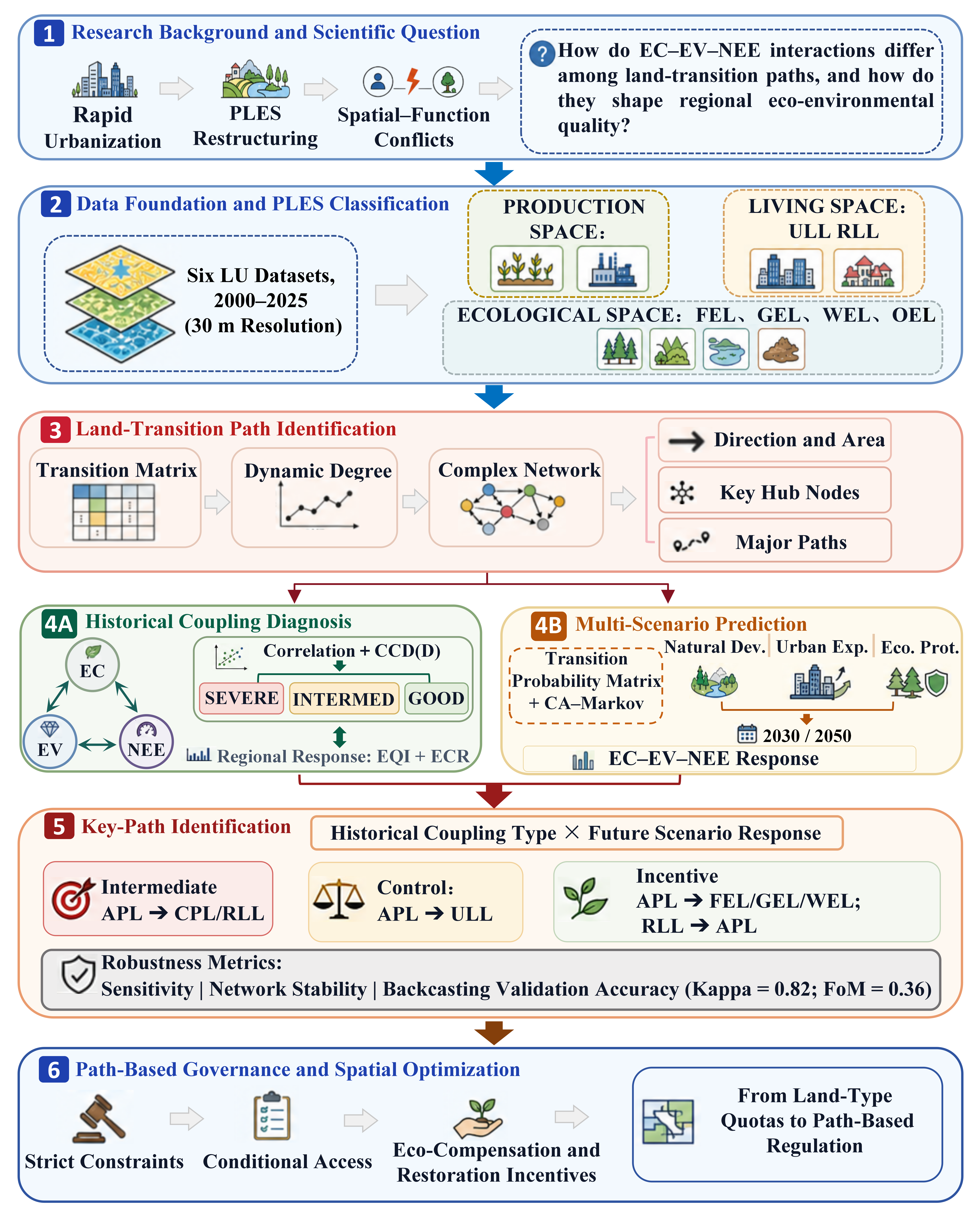
Wenjiang District is located in the central Chengdu Plain and forms an important peri-urban transition area west of Chengdu’s central city. It is also situated within the broader implementation context of Chengdu’s Park City initiative and the green transformation of metropolitan agriculture [42,43]. The district has flat terrain, and metropolitan agriculture, ecological protection, industrial development, and residential functions coexist. In recent years, agricultural production space has contracted, urban living space has expanded, and the limited ecological space has faced increasing local fragmentation. These frequent functional transitions make Wenjiang a suitable case for examining land-use transition pathways and their eco-environmental effects in a peri-urban transition zone of a megacity. The historical analysis covers the period from 2000 to 2025, and the scenario simulations cover the period from 2030 to 2050. To address the central scientific question stated above, this study examines three specific questions. First, what spatiotemporal patterns and network structures characterize PLES transitions in Wenjiang District? Second, how can EC, EV, and NEE be quantified for individual transition pathways, and what trade-offs, synergies, or imbalances occur among them? Third, how do eco-environmental effects vary among the three future scenarios, and which pathways should be prioritized for control, incentivized, or subject to conditional management? Figure 1 presents the analytical framework.

2. Materials and Methods

2.1. Study Area and Data

2.1.1. Study Area

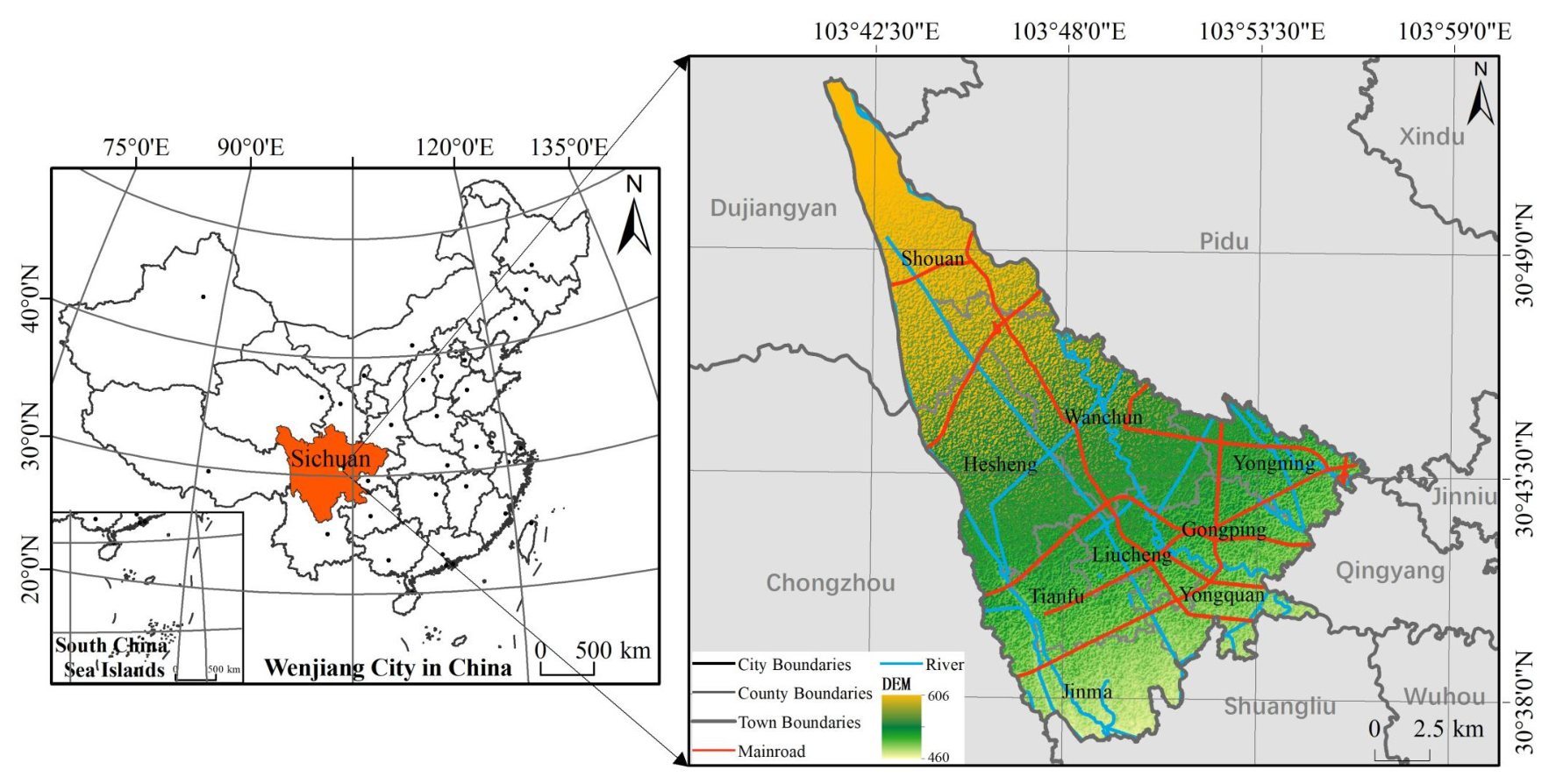
Wenjiang District is located in the central Chengdu Plain between 103°41′ E and 103°55′ E and between 30°36′ N and 30°52′ N. Its elevation ranges from approximately 408.3 to 642.4 m, and its total area is approximately 277 km² (Figure 2). The district has flat terrain, a well-developed water system, and a mild, humid climate. It comprises six subdistricts, namely Liucheng, Tianfu, Jinma, Yongquan, Gongping, and Yongning, and three towns, namely Shou’an, Hesheng, and Wanchun. Wenjiang accommodates the westward expansion of Chengdu’s central urban area while supporting urban agriculture, ecological protection, and residential development. In recent years, agricultural production space has continued to contract, urban living space has expanded, and pressure from ecological-space fragmentation has increased. These frequent PLES transitions make Wenjiang a suitable case for examining land-use transition pathways and their ecological effects in the peri-urban transition zone of a megacity.

2.1.2. Data Sources and Processing

This study used three types of data comprising land-use, base geographic, and socioeconomic data. Land-use maps for 2000, 2005, 2010, 2015, 2020, and 2025 were obtained from the China Multi-Period Land Use Remote Sensing Monitoring Dataset (CNLUCC), published by the Resource and Environment Science and Data Center of the Chinese Academy of Sciences (https://www.resdc.cn/), at a spatial resolution of 30 m × 30 m. The dataset has an overall accuracy greater than 90% and a Kappa coefficient greater than 0.85 at the first classification level, while its accuracy at the second classification level is approximately 85% to 90%. It therefore meets the requirements for identifying the principal functional land-use classes and analyzing spatiotemporal land-use change and ecological effects in Wenjiang District. Base geographic data, including the administrative boundary, were obtained from the National Geomatics Center of China (https://www.ngcc.cn/) and used to define the study extent and support spatial analysis. Socioeconomic data were obtained from the Statistical Bulletin on the National Economic and Social Development of Wenjiang District, Chengdu, and used to describe the regional context of urbanization and land-use change.

Data processing and analysis were performed using ArcGIS10.8, QGIS 3.44.14 (QGIS Development Team), and Python. ArcGIS and QGIS were used primarily for spatial clipping, reclassification, area calculation, and map preparation. Python 3.10 was used for weight sensitivity analysis, network metric calculation, coupling coordination analysis, Markov matrix operations, CA spatial allocation, and statistical visualization. Numerical and array operations used NumPy 1.26.4, neighborhood calculations used SciPy 1.13.1, and raster input and output used Rasterio 1.3.10. Network analysis used NetworkX 3.3, while tabular data were managed with pandas 2.2.2 and openpyxl 3.1.5. The transition probability matrices, sensitivity analyses, coupling analyses, and model validation results are provided in Supplementary Tables S1–S7 and Supplementary Figures S1–S4. The spatial allocation inputs and CA configuration used in the CA–Markov simulations are summarized in Supplementary Table S7.

2.2. Methods

2.2.1. Classification of PLES Functional Land-Use Classes and Eco-Environmental Quality Weights

Functional land-use classes were defined according to the dominant production, living, and ecological functions of land. The classification draws on previous studies of PLES multifunctionality, functional identification, and eco-environmental effects [7,8,13,15]. On this basis, in light of the land-use characteristics of Wenjiang District, we classified land into three primary categories comprising production, living, and ecological spaces, and eight secondary categories comprising APL, CPL, ULL, RLL, FEL, GEL, WEL, and OEL.

Table 1. Classification system and eco-environmental quality weights for PLES functional land use.

Classification by Dominant Land-Use Function		Corresponding CNLUCC Land-Use Type	Eco-Environmental Quality Weight
First-Level PLES Category	Functional Land-Use Class
Production space	Agricultural production land	Paddy fields and dry cropland	0.25
	Construction production land	Other construction land	0.05
Ecological space	Forest ecological land	Forestland, shrubland, sparse woodland, and other woodland	0.85
	Grassland ecological land	High-, medium-, and low-coverage grassland	0.65
	Water ecological land	Rivers and canals, lakes, reservoirs and ponds, glaciers and permanent snow, tidal flats, and floodplains	0.35
	Other ecological land	Sandy land, marshland, bare land, bare rock, and other unused land	0.15
Living space	Urban living land	Urban land	0.08
	Rural living land	Rural settlements	0.12

presents the correspondence between these categories and the original land-use classes. The first level consists of production, living, and ecological spaces. The second level comprises eight classes: agricultural production land (APL), construction production land (CPL), urban living land (ULL), rural living land (RLL), forest ecological land (FEL), grassland ecological land (GEL), water ecological land (WEL), and other ecological land (OEL).

The eco-environmental quality weights for the eight functional land-use classes were developed with reference to recent PLES assessments of eco-environmental quality [13,14,16]. Experts in land use, ecological assessment, and territorial spatial planning constructed the AHP pairwise comparison matrix, using the 1 to 9 scale proposed by Saaty [44]. The final weights are reported in Table 1, and the judgment matrix and consistency test are provided in Supplementary Table S1. To assess the sensitivity of the main findings to changes in the eco-environmental quality weights, two perturbation levels of ±10% and ±20% were used. The ±10% perturbation represents local variation around each baseline weight, whereas the ±20% perturbation tests whether the temporal trend in the EQI remains stable under a broader departure from the baseline. One functional land-use weight was varied at a time, while all other weights were held constant, and the EQI was recalculated for each year. Each weight was then assumed to follow a triangular distribution with the baseline value as the mode, and 80% and 120% of the baseline value as the lower and upper bounds. This distribution concentrates the samples near the baseline while allowing bounded variation in both directions. A total of 1000 Monte Carlo samples were generated, and the 2.5th and 97.5th percentiles were used to estimate the 95% interval of the EQI. This analysis tests the robustness of the temporal trend and relative ranking to changes in the weights. The results are reported in Supplementary Table S2 and Supplementary Figure S1.

2.2.2. Analysis of Transitions Among PLES Functional Land-Use Classes

The land-use transition matrix is a fundamental tool for analyzing the spatiotemporal evolution of PLES. It quantitatively records the direction and magnitude of transitions among land-use classes during the study period. Based on the transition matrix, this study characterizes land-use transitions from two dimensions: the rate of change and the network structure.

The land-use dynamic degree describes the rate and structural characteristics of land-use change over a given period. It includes the individual and comprehensive land-use dynamic degrees. The individual land-use dynamic degree represents the mean annual rate of change in a specific land-use class during the study period and is calculated as follows:

$$K={\displaystyle \frac{U_b-U_a}{U_a}}\times {\displaystyle \frac{1}{T}}\times 100\%$$

(1)

where $K$ is the dynamic degree of a specific land-use class during the study period; $U_b$ and $U_a$ are the areas of that land-use class at the end and beginning of the study period, respectively; and $T$ is the duration of the study period. The comprehensive land-use dynamic degree represents the overall intensity of regional land-use change based on transitions among all land-use classes and is calculated as follows:

$$LC=\left[{\displaystyle \frac{{\displaystyle {\sum }_{i=1}^n}{∆LU}_{i-j}}{2{\displaystyle {\sum }_{i=1}^n}{LU}_i}}\right]\times {\displaystyle \frac{1}{T}}\times 100\%$$

(2)

where $LC$ is the comprehensive land-use dynamic degree; ${LU}_i$ is the area of land-use class $i$ at the beginning of the study period; ${∆LU}_{i-j}$ is the absolute area of land-use class $i$ converted to land-use classes other than $i$ during the study period; and $T$ is the duration of the study period.

Building on the transition matrix, this study applies complex network theory [17,18] to construct a weighted directed network in which land-use classes are represented as nodes, transitions are represented as directed edges, and transition areas are used as edge weights. The network characterizes the topology of land-use transition pathways and identifies critical nodes and major transition pathways using the number of nodes, number of edges, network density, average clustering coefficient, average path length, and degree centrality. Because the network structure may evolve over time, separate networks are constructed for 2000–2010 and 2010–2025. Differences in their topological characteristics are compared to assess the temporal stability of the network structure. The network diagrams and topological metrics for the two periods are provided in Supplementary Figure S2 and Supplementary Table S5, respectively.

2.2.3. Quantitative Assessment of Eco-Environmental Effects

The EQI characterizes the eco-environmental quality of an evaluation unit by combining the area share and eco-environmental quality weight of each functional land-use class [13,14,15,16]. It is calculated as follows:

$${EQI}_k={\displaystyle \sum _{i=1}^n}{\displaystyle \frac{S_{ki}}{S_k}}\times T_i$$

(3)

where ${EQI}_k$ is the EQI of evaluation unit $k$; $S_{ki}$ is the area in evaluation unit $k$ of functional land-use class $i$; $S_k$ is the total land area of evaluation unit $k$; $T_i$ is the eco-environmental quality weight of functional land-use class $i$ as presented in Table 1; and $n$ is the number of PLES functional land-use classes. The calculated $EQIₖ$ values were classified into five levels using the Natural Breaks (Jenks) method, namely low, relatively low, moderate, relatively high, and high. To ensure comparability across years, the natural breakpoints obtained for 2000 were used as fixed thresholds for all subsequent years.

The ECR quantifies the contribution of functional land-use transitions to regional eco-environmental quality. Positive values indicate improvement, whereas negative values indicate degradation [13,14,15,16]. It is calculated as follows:

$$\mathit{ECR}={\displaystyle \frac{\left({EQI}_j-{EQI}_i\right)\times LA}{TA}}$$

(4)

where the ECR is the ecological contribution rate of a functional land-use transition; $EQIᵢ$ and $EQIⱼ$ are the eco-environmental quality indices assigned to the corresponding land-use classes before and after the transition, respectively; $LA$ is the transition area; and $TA$ is the total area of functional land use. An ECR greater than zero indicates an improvement in eco-environmental quality, whereas an ECR less than zero indicates degradation.

In addition to the EQI and ECR, this study evaluates the ecological effects of functional land-use transitions across three dimensions, namely EC, EV, and NEE. The land-use classes are represented as network nodes, and directed transitions between classes are represented as edges. For a directed transition edge l from functional land-use class $i$ to class $j$, the changes in ecological cost and ecological value associated with the pathway are calculated using Equations (5) and (6), respectively,

$$∆E{C}_l=({EC}_j-{EC}_i)S_l$$

(5)

$${∆EV}_l=\left(e_j-e_i\right)S_l$$

(6)

where $i$ and $j$ denote the source and destination functional land-use classes, respectively; $l$ denotes a directed transition edge from $i$ to $j$, which is treated as a specific land-use transition pathway; ${EC}_i$ and ${EC}_j$ are the ecological cost coefficients of the source and destination classes, respectively; $e_i$ and $e_j$ are the ecosystem service value equivalent coefficients per unit area for the source and destination classes, respectively; and $S_l$ is the gross transition area of pathway $l$, measured in km². ${\Delta EC}_l$ is the change in ecological cost associated with pathway $l$. A positive value indicates an increase in ecological cost after the transition, whereas a negative value indicates a decrease. ${\Delta EV}_l$ is the change in ecological value associated with pathway $l$. A positive value indicates a gain in ecological value, whereas a negative value indicates a loss [45,46]. For concise presentation, ${\Delta EC}_l$ and ${\Delta EV}_l$ are referred to as EC and EV, respectively, in subsequent pathway analyses, figures, and tables. The ecological cost coefficients and ecosystem service value equivalent coefficients of the functional land-use classes are listed in

Table 2. The ecological cost coefficients and ecosystem service value-equivalent coefficients for the functional land-use classes.

Functional Land-Use Class	Ecological Cost Coefficient	Ecosystem Service Value-Equivalent Coefficient
Agricultural production land	100	7.9
Construction production land	1000	0
Forest ecological land	5	28.12
Grassland ecological land	22	11.67
Water ecological land	5	45.35
Urban living land	1000	0
Rural living land	600	0

Note: OEL is excluded from the calculations because its area is zero throughout the study period.

.

Network ecological efficiency (NEE) in this study is defined for the land-use transition network and characterizes pathway performance in terms of ecological value change relative to ecological cost change, together with its aggregation at the network level [27]. Reference [27] introduced NEE for land-use transition networks. Because this study compares specific transition pathways whose transition areas differ substantially, we operationalized this network concept at the pathway scale. Differences in EC and EV coefficients between the source and destination classes are weighted by gross transition area, and the contribution of transition pathway $l$ to network ecological efficiency is defined as follows:

$${NEE}_l={\displaystyle \frac{{\Delta EV}_l}{\left(\left|{\Delta EC}_l\right|+1\right)}}$$

(7a)

where ${NEE}_l$ is the signed contribution of pathway $l$, expressed as the ecological value change relative to the magnitude of ecological cost change. The $+1$ term in the denominator prevents division by zero when ${\Delta EC}_l = 0$. Because the denominator is always positive, the sign of ${NEE}_l$ is determined by ${\Delta EV}_l$. A positive value indicates an ecological value gain, whereas a negative value indicates an ecological value loss. Its absolute value represents the magnitude of ecological value change relative to ecological cost change within the weighting system used in this study. ${NEE}_l$ for a single pathway is a pathway-level contribution to network ecological efficiency and does not represent the overall efficiency of the entire network.

At the network level, the contributions of individual pathways are aggregated along minimum ecological cost paths to obtain an overall network indicator.

$${NEE}_{net}={\displaystyle \frac{1}{N\left(N-1\right)}}\times \sum _{\begin{array}{c}i,j\in N\\ i\ne j\end{array}}\sum _{l\in L_{ij}^{min}}{NEE}_l$$

(7b)

where $\mathcal{N}$ is the set of network nodes and $N = \left|\mathcal{N}\right|$ is the number of nodes. $L_{ij}^{min}$ is the set of directed edges on the minimum ecological cost path from node $i$ to node $j$, where the path minimizes the sum of $\left|{\Delta EC}_l\right|$ across its edges. ${NEE}_{net}$ is the overall network ecological efficiency obtained by aggregating pathway contributions. Equation (7a) defines the individual pathway contribution used in the inner summation of Equation (7b), while Equation (7b) aggregates these contributions over the minimum ecological cost paths for all ordered node pairs. ${NEE}_l$ and ${NEE}_{net}$, therefore, represent two levels of the same computational framework. ${NEE}_l$ is not a separate efficiency indicator independent of the network definition and should not be interpreted as the overall efficiency of the entire network. Because specific transition pathways are the principal units of analysis in this study, unsubscripted NEE in subsequent pathway results, figures, tables, correlation analysis, and coupling coordination analysis refers to ${NEE}_l$. ${NEE}_{net}$ is used only for the network-level indicator. NEE is a relative index constructed from weighted coefficients for comparisons within the same evaluation system. It is not interpreted as an energy conversion efficiency with physical units.

2.2.4. Coupling Coordination Analysis of Ecological Cost, Value, and Efficiency

The joint analysis of EC, EV, and NEE compares the relative states of land-use transition pathways across the cost, value, and efficiency dimensions [28,29]. NEE is the pathway-level contribution, ${NEE}_l$, calculated using Equation (7a). Spearman rank correlations are first used to evaluate the pairwise relationships among EC, EV, and NEE across the 31 direct transition pathways. The coupling coordination degree model is then used to characterize the relative positions and balance of the three indicators after their directions have been aligned. Because ${NEE}_l$ is derived from EC and EV; the correlation coefficients and coupling coordination degree describe statistical associations and joint distributional patterns. They are not used to identify causal coupling among three independent systems.

EC, EV, and NEE differ in scale and direction. Each indicator is, therefore, range-normalized using the sample minimum and maximum across the 31 direct transition pathways and mapped to the interval from 0.01 to 1.00. EC is treated as a negative indicator, whereas EV and NEE are treated as positive indicators. The normalized values are calculated as follows:

$${EC}_l^{\prime }=0.01+0.99\times {\displaystyle \frac{{EC}_{max}-{EC}_l}{{EC}_{max}-{EC}_{min}}}$$

(8)

$${EV}_l^{\prime }=0.01+0.99\times {\displaystyle \frac{{EV}_l-{EV}_{min}}{{EV}_{max}-{EV}_{min}}}$$

(9)

$${NEE}_l^{\prime }=0.01+0.99\times {\displaystyle \frac{{NEE}_l-{NEE}_{min}}{{NEE}_{max}-{NEE}_{min}}}$$

(10)

where ${EC}_l$, ${EV}_l$, and ${NEE}_l$ are the raw EC, EV, and NEE values for pathway $l$. ${EC}_{min}$, ${EV}_{min}$, and ${NEE}_{min}$ are the respective sample minima across the 31 pathways, while ${EC}_{max}$, ${EV}_{max}$, and ${NEE}_{max}$ are the respective sample maxima. ${EC}_l^{\prime }$, ${EV}_l^{\prime }$, and ${NEE}_l^{\prime }$ are the direction-aligned normalized values. The lower bound of 0.01 and the scaling factor of 0.99 map each indicator to the interval from 0.01 to 1.00. This prevents the product in Equation (8) from becoming zero when an indicator reaches its sample minimum. The transformation preserves the within-sample rank order of each indicator, but the normalized values and the resulting $C$ and $D$ depend on the range of pathways included in this study.

The coupling degree C and coupling coordination degree $D$ are calculated as follows:

$$C={\displaystyle \frac{3\times \sqrt[3]{{EC}_l^{\prime }\times {EV}_l^{\prime }\times {NEE}_l^{\prime }}}{{EC}_l^{\prime }+{EV}_l^{\prime }+{NEE}_l^{\prime }}}$$

(11)

$$D=\sqrt{C\times T}$$

(12)

The comprehensive development index $T$ is calculated as $T = \alpha {EC}_l^{\prime } + \beta {EV}_l^{\prime } + \gamma {NEE}_l^{\prime }$. EC, EV, and NEE represent the cost, value, and efficiency dimensions of land-use transitions, respectively, and provide complementary information. The available evidence does not justify assigning greater importance to any one dimension. Equal weights are, therefore, applied after direction alignment and normalization, with $\alpha =\beta =\gamma =1/3$, as a neutral specification without an additional preference structure. This setting is used only to calculate $T$ and $D$ and does not change the raw EC, EV, or NEE value of any pathway. $C$ measures the relative balance among the three normalized values and approaches 1 as the values become more similar. $T$ represents their weighted mean level. $D$ combines $C$ and $T$ to compare the relative coordination of pathways within the same normalized evaluation set. A higher $D$ does not necessarily indicate a greater absolute ecological gain and does not, by itself, demonstrate a causal interaction among EC, EV, and NEE [28].

Five relative coordination levels are defined from $D$. Severe imbalance corresponds to $0\le D<0.2$, mild imbalance to $0.2\le D<0.4$, basic coordination to $0.4\le D<0.6$, moderate relative coordination to $0.6\le D<0.8$, and good relative coordination to $0.8\le D\le 1.0$ [47]. These labels support relative comparisons within the same evaluation set. Their interpretation must also consider the raw EC, EV, and NEE values. The Spearman correlation coefficients, $C$, $D$, and relative coordination levels of all pathways are reported in Supplementary Table S4. The D values of the major pathways are provided in Supplementary Figure S3 and Supplementary Table S4.

2.2.5. Multi-Scenario Simulation of PLES Functional Land-Use Change

This study defines natural development, urban expansion, and ecological protection scenarios to compare the potential ecological effects of land-use change under different development assumptions. The natural development scenario retains the baseline probability matrix calculated from historical land-use transitions between 2000 and 2025, and represents a continuation of the historical transition structure. The urban expansion scenario represents stronger pressure from urban expansion. The magnitude and intensity of the major urbanization-related transitions during the historical period, together with the planned increase in construction land in the Chengdu Territorial Spatial Master Plan for 2021 to 2035, were used to define the adjustments. Before row normalization, the baseline probabilities of APL→ULL, APL→CPL, and RLL→ULL were multiplied by 1.25, 1.20, and 1.15, respectively. The direction of adjustment under the ecological protection scenario was based on the plan’s requirements for cropland protection, ecological-space conservation, and the urban development boundary. Before row normalization, the baseline probabilities of APL→ULL and APL→CPL were multiplied by 0.65 and 0.70, while those of APL→FEL and APL→GEL were multiplied by 1.60 and 1.30, respectively. Transitions out of FEL, GEL, and WEL were further restricted. The removed probability mass was assigned to retention in the original class, increasing the retention probabilities of these three ecological classes to 0.9386, 0.7727, and 0.9547, respectively. Transition relationships not targeted for adjustment retained their baseline relative proportions.

After the scenario-specific adjustments, each row of the transition matrix was normalized so that the probabilities across all destination classes summed to one. Historical land-use change and planning requirements were used to identify the pathways and directions of constraint. The multipliers define comparable conditional scenarios. They do not imply a direct numerical conversion between planning targets and transition probabilities and are not deterministic forecasts of future land-use patterns. The final row-normalized probability matrices are reported in Supplementary Table S3.

The prediction of land-use structure under the three scenarios is driven by the Markov chain model [31], while their spatial distributions are simulated using the CA–Markov framework [32,33]. The Markov chain model calculates the baseline transition probability matrix from the land-use transition matrices for the periods between 2000 and 2025. The transition probability $P_{ij}$ is calculated as follows:

$$P_{ij}={\displaystyle \frac{T_{ij}}{{\sum }_{j=1}^n{T}_{ij}}}\left(0\le P_{ij}\le 1, {\displaystyle \sum _{j=1}^n}{P}_{ij}=1\right)$$

(13)

where $T_{ij}$ represents the area converted from functional land-use class $i$ in the initial period to functional land-use class $j$ in the final period. The $P_{ij}$ satisfies $0\le P_{ij}\le 1$ and $\sum P_{ij}=1$. If $S_t$ denotes the state vector of functional land-use areas at time $t$, the land-use structures for the next period and multiple subsequent periods are projected as follows:

$$S_{t+1}=S_{t}P$$

(14)

$$S_{t+k}=S_t{P}^k$$

(15)

where $P$ is the transition probability matrix, and $k$ is the number of five-year projection steps. Future simulations used the 2025 PLES functional land-use grid at 30 m resolution as the initial state. The 2030 and 2050 projections correspond to one and five steps, respectively. At each step, the Markov model calculates the target quantity of each functional land-use class as $S_{t+1}=S_t{P}^{\left(s\right)}$, where $P^{\left(s\right)}$ is the row-normalized transition probability matrix for scenario $s$. The matrix remained constant over the projection period of that scenario.

No external topographic, transport, or socioeconomic suitability variables were used, and no weights were assigned to external variables. Spatial allocation depends only on the scenario-specific transition probability and the neighborhood of the destination class. For a candidate cell $x$ in class $i$ at time $t$, the neighborhood proportion of destination class $j$ is calculated as follows.

$${\Omega }_j\left(x,t\right)={\displaystyle \frac{{\sum }_{y\in N_{5\times 5}\left(x\right),y\ne x}I\left[z\left(y,t\right)=j\right]}{n_x}}$$

(16)

The corresponding spatial allocation score is calculated as follows:

$$A_{ij}^{\left(s\right)}\left(x,t\right)=p_{ij}^{\left(s\right)}\times {\Omega }_j\left(x,t\right)$$

(17)

where $N_{5\times 5}\left(x\right)$ is the 5 × 5 Moore neighborhood of cell $x$, $z\left(y,t\right)$ is the functional land-use class of neighboring cell $y$ at time $t$, and $I\left[\cdot \right]$ is an indicator function. The term $n_x$ is the number of valid neighboring cells after excluding the center cell and NoData cells outside Wenjiang District. For an interior cell, $n_x$ = 24. The term ${\Omega }_j\left(x,t\right)$ is the proportion of valid neighboring cells assigned to destination class $j$, $p_{ij}^{\left(s\right)}$ is the probability of transition from class $i$ to class $j$ under scenario $s$, and $A_{ij}^{\left(s\right)}\left(x,t\right)$ is the resulting spatial allocation score.

At each five-year step, only transitions with $p_{ij}^{\left(s\right)}>0$ were treated as candidates. The spatial allocation scores were first calculated from the current land-use state, after which candidate cells were allocated in descending order of their scores. A cell could be allocated only once during a time step. Allocation to a destination class stopped when the target number of cells specified by the Markov model had been reached, and all cell states were then updated synchronously. Tied scores were resolved using the fixed row and column order of the input grid. No stochastic perturbation or random seed was used. All three scenarios used the same initial map, neighborhood configuration, time step, and spatial allocation procedure. Only the row-normalized transition probability matrix differed among scenarios, which maintained comparability [30,31,32,33]. The complete configuration is reported in Supplementary Table S7.

Model reliability was evaluated through backcasting. The backcasting simulations used the same 30 m grid, 5 × 5 Moore neighborhood, five-year time step, and synchronous spatial allocation rule as the future scenarios. A five-year baseline transition probability matrix was calculated from the 2000, 2005, and 2010 land-use data. The 2010 PLES functional land-use map was then used as the initial state, and the model was run for one, two, and three steps to simulate the patterns observed in 2015, 2020, and 2025, respectively. The simulated maps were compared with the observed maps for the corresponding years, and the Kappa coefficient and Figure of Merit (FoM) were calculated [48,49]. Kappa measures overall agreement between a simulated map and its observed counterpart. FoM is the proportion of correctly simulated changed cells relative to the union of observed and simulated change. Supplementary Table S6 also reports the overall area R² and the user’s and producer’s accuracies for each functional land-use class, allowing model performance to be assessed in terms of both quantity and spatial allocation.

3. Results

3.1. Spatiotemporal Evolution and Network Structure of PLES Functional Land Use

3.1.1. Structure and Spatial Changes in PLES Functional Land Use

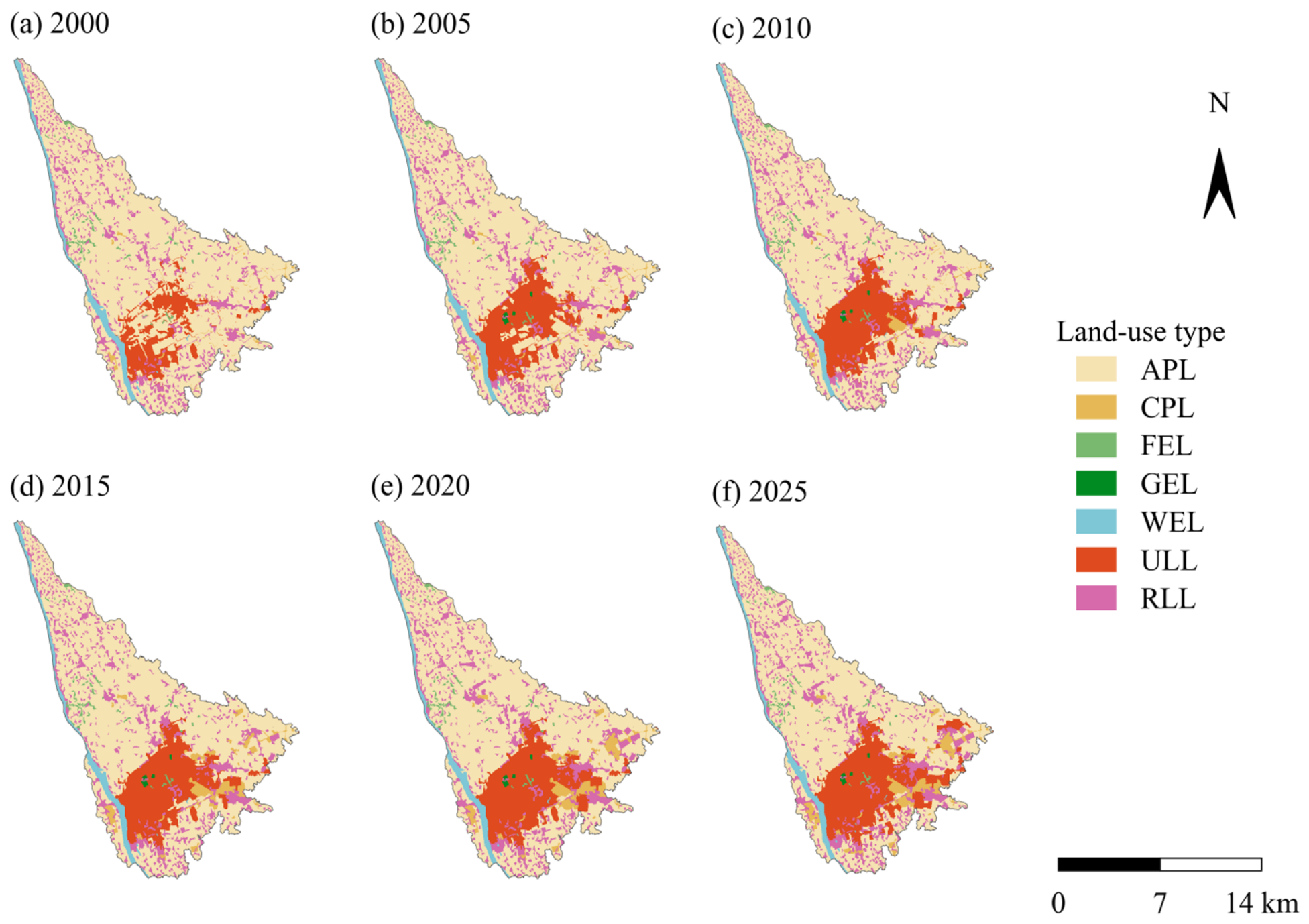
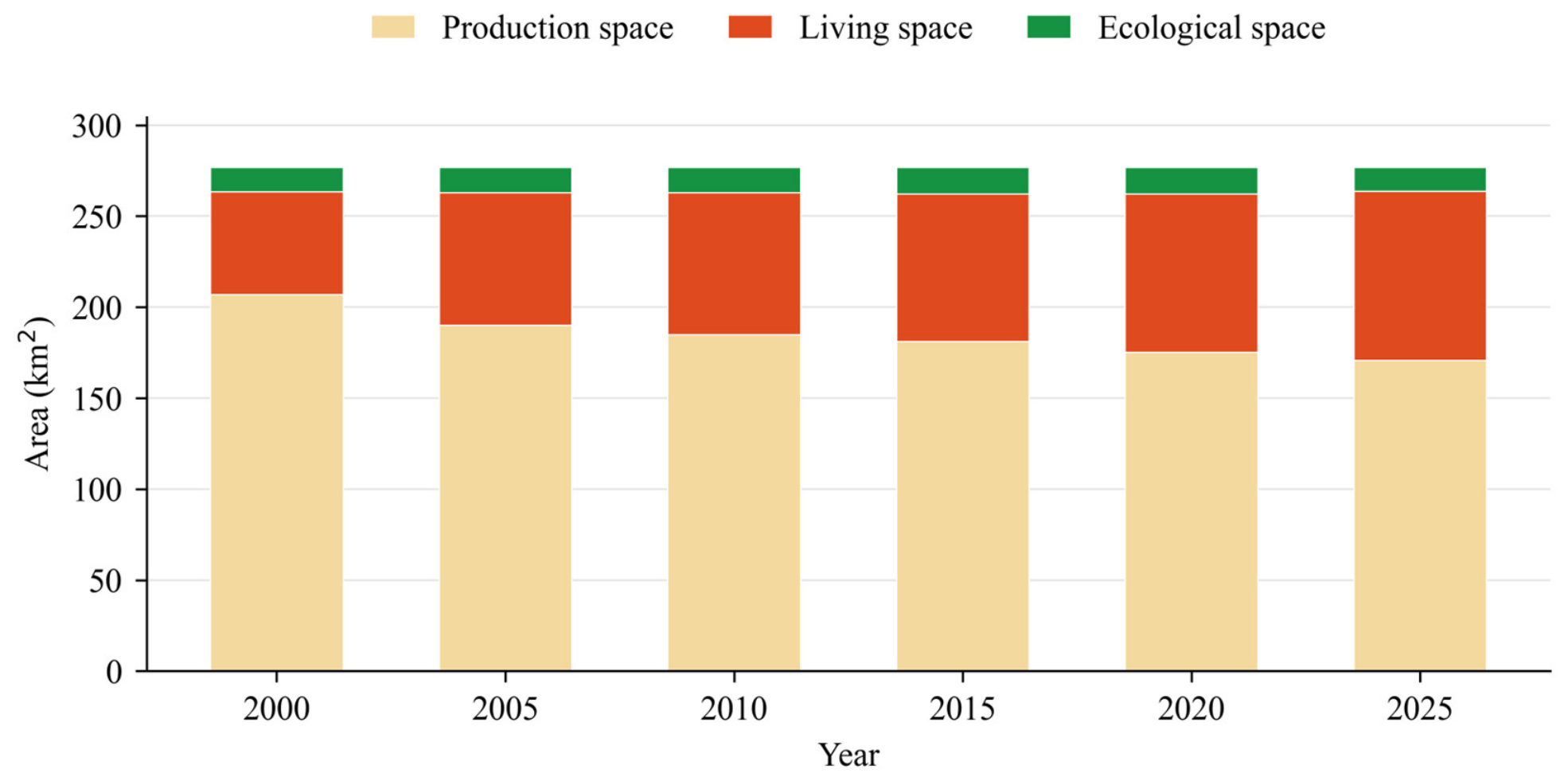
Between 2000 and 2025, PLES restructuring in Wenjiang District was characterized primarily by the continued conversion of agricultural production space into living space. Production space remained dominant throughout the study period, although its share continuously declined. Living space steadily expanded, whereas ecological space accounted for a relatively small proportion and changes only slightly. Spatially, APL remained the dominant functional land-use class and wass concentrated in the western and northern towns of Shou’an, Hesheng, and Wanchun (Figure 3). These areas support much of the urban agriculture serving western Chengdu. ULL was concentrated mainly in the southeastern subdistricts of Liucheng, Tianfu, Jinma, Yongquan, Gongping, and Yongning. RLL was dispersed within APL, while CPL occured mainly in the southeast. FEL was distributed primarily along the northwestern boundary and in the central–western part of the district, where it forms fragmented and scattered patches. GEL and WEL occurred sporadically along rivers and channels. Given the flat terrain of Wenjiang, production and living spaces together accounted for most of the district, while OEL was negligible.

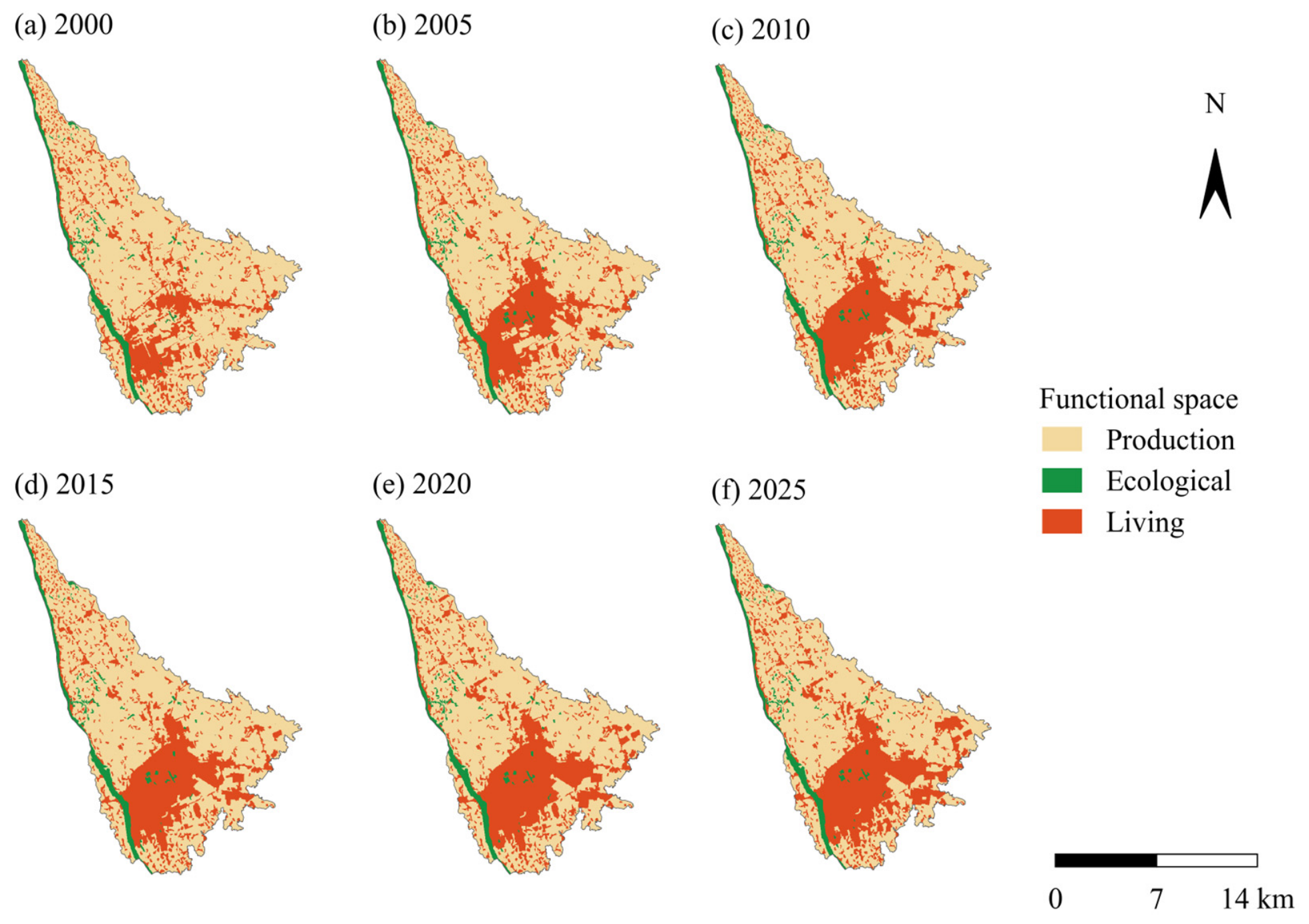
At the level of the three major PLES categories, living space continuously expanded outward from the central and southeastern parts of the district between 2000 and 2025 (Figure 4). The areas of both ULL and RLL increased, while production space contracted accordingly. The overall pattern of ecological space remained relatively stable. However, FEL initially increased slightly and then gradually decreased, accompanied by the further fragmentation of some local patches.

Changes in area composition further confirm these trends (Figure 5). The proportion of production space declined continuously, whereas that of living space increased steadily, showing a clear inverse pattern. Ecological space remain limited and exhibited only minor fluctuations. This pattern is consistent with the continued conversion of agricultural production space to living space, while the small ecological-space base showed no marked structural expansion during the study period.

3.1.2. Dynamic Degree of PLES Functional Land-Use Change

Land-use dynamic degrees in Wenjiang District exhibit pronounced temporal fluctuations, with 2000–2005 and 2010–2015 representing two periods of particularly active change. The mean comprehensive land-use dynamic degree (LC) across the five monitoring intervals is 0.506%. The LC values are 0.631% for 2000–2005, 0.238% for 2005–2010, 0.907% for 2010–2015, 0.283% for 2015–2020, and 0.473% for 2020–2025. LC reached its highest value during 2010–2015, followed by 2000–2005, and both values are substantially higher than those of the other intervals (

Table 3. Dynamic degrees of PLES functional land-use classes in Wenjiang District, 2000–2025.

Period	Individual Dynamic Degree, K (%)								Comprehensive Dynamic Degree, LC (%)
	APL	CPL	FEL	GEL	WEL	OEL	ULL	RLL
2000–2005	−1.706	6.262	0.586	325.806	0.003	–	11.684	1.452	0.631
2005–2010	−0.702	9.563	0.000	0.000	0.000	–	2.544	0.236	0.238
2010–2015	−0.986	24.641	−0.056	0.000	1.157	–	0.574	1.024	0.907
2015–2020	−0.905	3.682	0.000	0.000	−0.093	–	1.372	1.646	0.283
2020–2025	−0.640	1.422	0.348	0.336	−2.332	–	2.175	0.321	0.473

). In terms of fluctuations in individual land-use categories, ULL and CPL exhibit the most dramatic fluctuations. The rapid expansion of ULL is concentrated in 2000–2005, when its single land-use dynamic degree reached 11.684%. This period coincides with accelerated urbanization in Wenjiang, as Chengdu advanced its southward urban development strategy and redistributed functions from its central urban area, after which the expansion gradually stabilized. The sharp increase in CPL is concentrated in 2010–2015, when its single land-use dynamic degree reached 24.641%. This period coincides with the industrial expansion associated with the decentralization of functions from central Chengdu and the concentration of healthcare industries and higher education resources in Wenjiang. Changes in ULL and CPL jointly contribute to the peaks in the comprehensive land-use dynamic degree during these two periods.

3.1.3. Network Structure of PLES Functional Land-Use Transitions

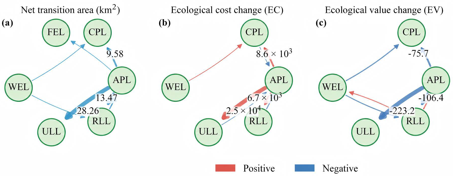
The land-use transition network in Wenjiang District is dominated by the APL→ULL pathway, with APL and ULL forming the principal hub nodes. The network exhibits distinct stages of evolution between 2000–2010 and 2010–2025. Across the entire 2000–2025 period, the net transition area along the APL→ULL pathway reached 28.26 km², substantially exceeding that of all other pathways (Figure 6a). It therefore represents the dominant direction of land-use transition during the study period. APL→CPL is the second-largest pathway, indicating that residential and industrial development jointly drive the conversion of agricultural production space. RLL→APL, which is associated with rural land consolidation and reclamation, represents the principal reverse pathway. The asymmetry among these pathways demonstrates that land-use transitions in Wenjiang are characterized mainly by the one-way conversion of agricultural production space, with limited reverse conversion.

To assess the temporal stability of the network structure, separate land-use transition networks were constructed for 2000–2010 and 2010–2025 (Supplementary Figure S2 and Supplementary Table S5). The 2000–2010 network contains six nodes and five edges, has a network density of 0.167, and identifies APL as its hub node. The 2010–2025 network contains seven nodes and 31 edges, has a network density of 0.738, and identifies ULL and RLL as its hub nodes. This shift from APL to ULL and RLL indicates that the center of the network moves from APL toward living land, although APL and ULL remain critical nodes in the major transition pathways. The greater number of pathways during the later period also indicates increasing diversification. The network evolves from a relatively concentrated pattern dominated by transitions between agricultural production and living spaces to a more complex structure in which multiple pathways coexist.

3.2. Eco-Environmental Effects and Coupling Characteristics of PLES Functional Land-Use Change

3.2.1. Spatiotemporal Evolution of Eco-Environmental Quality

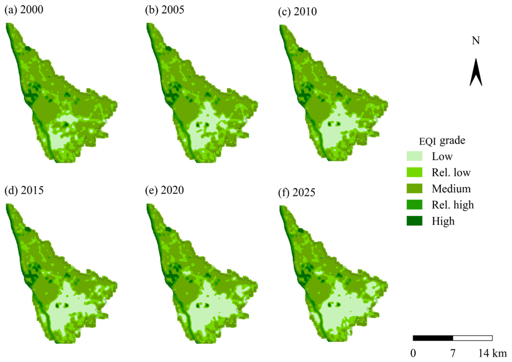
From 2000 to 2025, the EQI of Wenjiang District declined continuously from 0.228 to 0.200, a cumulative decrease of approximately 12.3%. Spatially, the EQI consistently followed a northwest-to-southeast gradient, with higher values in the northwest and lower values in the southeast. Areas with a moderate and relatively high EQI were concentrated mainly in Shou’an, Hesheng, and Wanchun, where APL was the dominant functional land-use class (Figure 7). Low-EQI areas occurred mainly in Tianfu and Liucheng, where ULL and CPL predominated. As living and construction spaces expanded, areas with a moderate and relatively high EQI contracted, while low-EQI areas expanded.

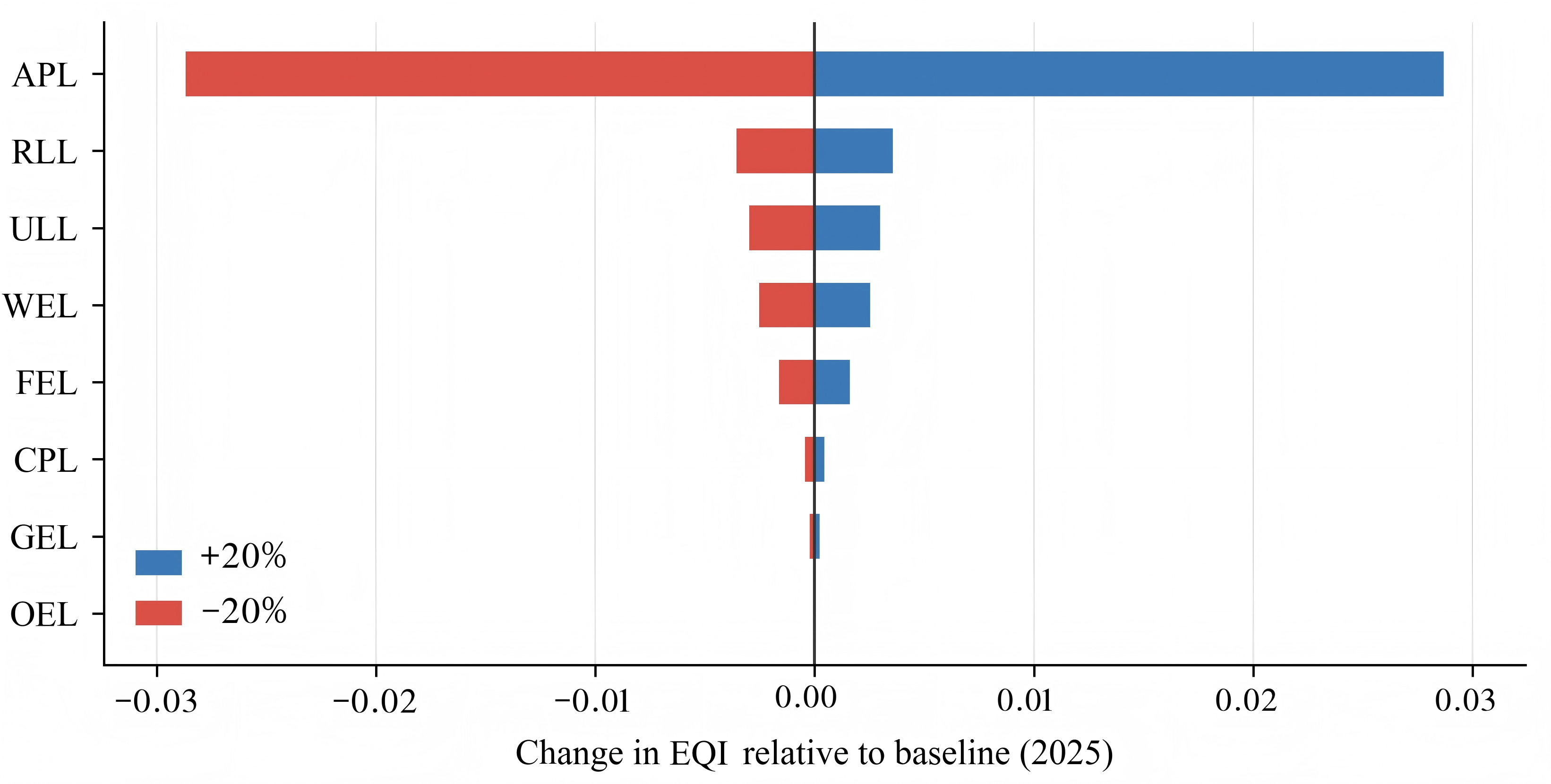
The EQI decreases in the five successive periods were 4.088%, 1.889%, 2.420%, 2.183%, and 2.133%, respectively. The largest decrease occurred from 2000 to 2005, coinciding with concentrated transitions from APL to ULL, RLL, and CPL. The EQI continued to decline from 2005 to 2025, although the decreases were generally smaller than those observed from 2000 to 2005, except for a few individual periods. The weight sensitivity analysis showed that the EQI declined from 2000 to 2025 under all 32 settings obtained by applying one-at-a-time perturbations of ±10% and ±20% to the weights of the eight functional land-use classes. The cumulative decline ranged from 10.1% to 13.5%, consistent in direction with the baseline decline of 12.3%. In the Monte Carlo simulation, the interquartile ranges and baseline estimates also shifted downward over time, although the 95% simulation intervals for adjacent years overlapped (Figure 8, Supplementary Figure S1 and Supplementary Table S2).

3.2.2. Ecological Contribution Rates and Major Degradation Pathways

Continued transitions from APL and ecological land to non-ecological land were the main pathways associated with the negative total ECR in every period. The total ECR values for the five periods from 2000 to 2025 were −0.01060, −0.00413, −0.00520, −0.00457, and −0.00436, respectively, consistent with the overall decline in the EQI (

Table 4. Functional land-use transitions and their ecological contribution rates in Wenjiang District, 2000–2025.

Study Period	Transition Pathway	Converted Area (km2)	ECR	Effect
2000–2005	APL→FEL	0.0738	0.00016	Improvement
	Subtotal	0.0738	0.00016	Improvement
	APL→CPL	0.6876	−0.00050	Degradation
	APL→GEL	0.4545	−0.00066	Degradation
	APL→ULL	13.8654	−0.00852	Degradation
	APL→RLL	2.3805	−0.00112	Degradation
	Subtotal	17.3880	−0.01079	Degradation
	Total	17.4618	−0.0106	Degradation
2005–2010	APL→CPL	1.3788	−0.00100	Degradation
	APL→ULL	4.7817	−0.00294	Degradation
	APL→RLL	0.4149	−0.00019	Degradation
	Total	6.5754	−0.00413	Degradation
2010–2015	APL→FEL	0.4707	0.00102	Improvement
	APL→WEL	0.4428	0.00016	Improvement
	CPL→APL	0.3474	0.00025	Improvement
	CPL→ULL	0.1071	0.00001	Improvement
	CPL→RLL	0.1998	0.00005	Improvement
	ULL→APL	0.5031	0.00031	Improvement
	ULL→FEL	0.0639	0.00018	Improvement
	ULL→GEL	0.0513	0.00011	Improvement
	ULL→WEL	0.1251	0.00012	Improvement
	ULL→RLL	0.5013	0.00007	Improvement
	RLL→APL	5.2839	0.00248	Improvement
	RLL→FEL	0.0189	0.00005	Improvement
	RLL→GEL	0.0072	0.00001	Improvement
	RLL→WEL	0.4023	0.00033	Improvement
	Subtotal	8.5248	0.00516	Improvement
	APL→CPL	5.6421	−0.00408	Degradation
	APL→ULL	1.8099	−0.00111	Degradation
	APL→RLL	7.3908	−0.00347	Degradation
	FEL→APL	0.4410	−0.00096	Degradation
	FEL→WEL	0.0144	−0.00003	Degradation
	FEL→ULL	0.0639	−0.00018	Degradation
	FEL→RLL	0.0414	−0.00011	Degradation
	GEL→ULL	0.0495	−0.00010	Degradation
	GEL→RLL	0.0090	−0.00002	Degradation
	WEL→APL	0.2736	−0.00005	Degradation
	WEL→ULL	0.0261	−0.00003	Degradation
	WEL→RLL	0.0621	−0.00005	Degradation
	ULL→CPL	0.0990	−0.00002	Degradation
	RLL→CPL	0.1656	−0.00006	Degradation
	RLL→ULL	0.5040	−0.00007	Degradation
	Subtotal	16.5924	−0.0103	Degradation
	Total	25.1172	−0.00520	Degradation
2015–2020	APL→CPL	1.7514	−0.00127	Degradation
	APL→ULL	2.9898	−0.00184	Degradation
	APL→RLL	3.0258	−0.00142	Degradation
	WEL→RLL	0.0531	−0.00004	Degradation
	Total	7.8201	−0.00457	Degradation
2020–2025	APL→FEL	0.045	0.00010	Improvement
	APL→GEL	0.0081	0.00001	Improvement
	Subtotal	0.0531	0.00011	Improvement
	APL→CPL	0.124	−0.00009	Degradation
	APL→ULL	4.8121	−0.00296	Degradation
	APL→RLL	0.257	−0.00012	Degradation
	WEL→CPL	0.677	−0.00073	Degradation
	WEL→ULL	0.254	−0.00025	Degradation
	WEL→RLL	0.393	−0.00033	Degradation
	Subtotal	6.5171	−0.00447	Degradation
	Total	6.5702	−0.00436	Degradation

). The absolute total ECR was greatest from 2000 to 2005. During this period, 17.3880 km² of APL was converted to other land-use classes, including 13.8654 km² converted to ULL, indicating a close association between rapid urban expansion and the decline in eco-environmental quality. From 2010 to 2015, the summed ECR of improvement pathways reached its highest value of 0.00516, mainly because small areas were converted to forest, grassland, and water ecological land. The total ECR for this period nevertheless remained negative, indicating that the positive contributions of improvement pathways were insufficient to offset the effects of degradation pathways.

3.2.3. Ecological Cost, Ecological Value, and Network Ecological Efficiency of PLES Functional Land-Use Transitions

EC, EV, and NEE differed markedly among land-use transition pathways. APL→ULL produced the largest increase in EC at 25433.01, followed by APL→CPL at 8625.51, and APL→RLL at 6734.50 (Figure 6b and Supplementary Table S4). By contrast, the EC values for RLL→APL, APL→FEL, and APL→GEL were −2641.95, −56.00, and −36.08, respectively, indicating that these pathways were associated with reductions in ecological cost.

EV generally changed in the opposite direction to EC (Figure 6c and Supplementary Table S4). APL→ULL produced the greatest EV loss at −223.25, followed by APL→RLL at −106.41, and APL→CPL at −75.71. EV increased by 11.92, 16.58, and 41.74 along APL→FEL, APL→WEL, and RLL→APL, respectively, making these the principal value-enhancing pathways during the study period.

NEE, calculated as $NEE\mathrm{ₗ}$ using Equation (7a), also varied markedly among pathways. APL→ULL and APL→CPL both had an NEE of −0.00878. These negative values indicate ecological value losses along both pathways. By contrast, NEE was 0.20911 for APL→FEL and 0.38506 for APL→WEL. These positive values indicate ecological value gains and positive pathway-level contributions to network ecological efficiency.

3.2.4. Coupling Coordination of Ecological Cost, Value, and Efficiency in PLES Functional Land-Use Transitions

The coupling coordination degree of EC, EV, and NEE varied markedly among land-use transition pathways, with NEE calculated as ${NEE}_l$, using Equation (7a). Spearman correlation analysis showed a negative association between EC and EV $\left(\rho =-0.89\right)$ and a positive association between EV and NEE $\left(\rho =0.87\right)$ (Supplementary Table S4). Within the pathway sample, higher EC is generally associated with greater EV loss, whereas pathways with larger EV gains generally have higher NEE.

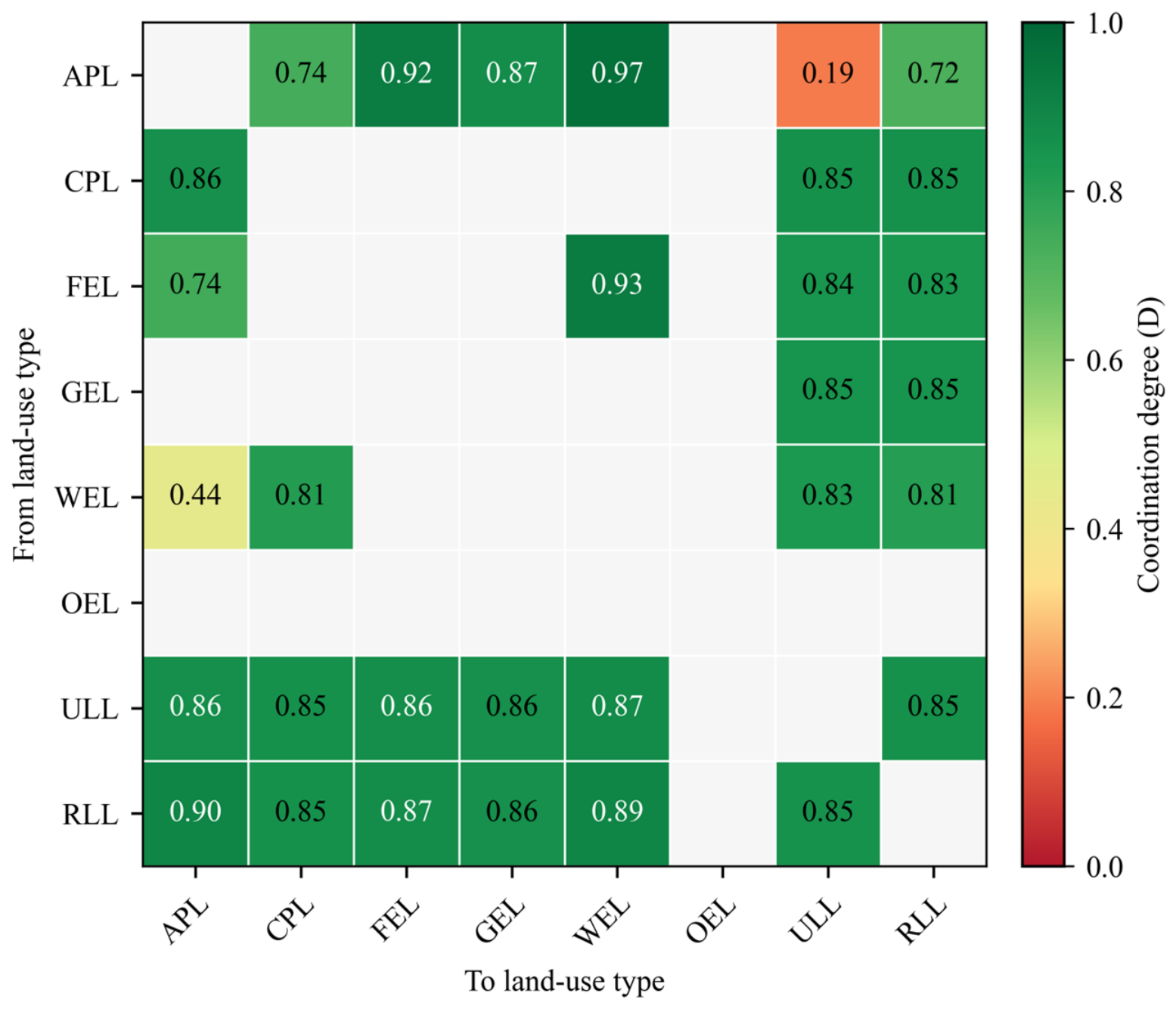
Figure 9 and Supplementary Table S4 show that APL→ULL had the lowest $D$ ($D$ = 0.191) and is classified as severely imbalanced. Its raw EC, EV, and NEE values were 25433.01, −223.25, and −0.00878, respectively. APL→CPL and APL→RLL had $D$ values of 0.741 and 0.724 and showed moderate relative coordination. For APL→CPL, the direction-aligned normalized values were $EC\prime$ = 0.6027, $EV\prime$ = 0.5612, and $NEE\prime$ = 0.4901. Their similarity produced $C$ = 0.996. Their mean level was $T$ = 0.551, which results in $D$ = 0.741. This level indicates that the three relative scores are comparatively balanced among the 31 pathways. However, the raw EC, EV, and NEE values remained as 8625.51, −75.71, and −0.00878, so the ecological effects of this pathway remain unfavorable. The $D$ values for APL→FEL, RLL→APL, APL→GEL, and APL→WEL were 0.924, 0.897, 0.870, and 0.968, respectively, indicating good relative coordination. These pathways also reduced ecological cost and increased ecological value. The results show that $D$ compares the relative balance of the normalized indicators, whereas the direction of ecological effects must be assessed from the raw EC, EV, and NEE values.

3.3. Multi-Scenario Simulation and Identification of Critical PLES Functional Land-Use Transition Pathways

3.3.1. Projected PLES Functional Land-Use Structure Under Three Scenarios

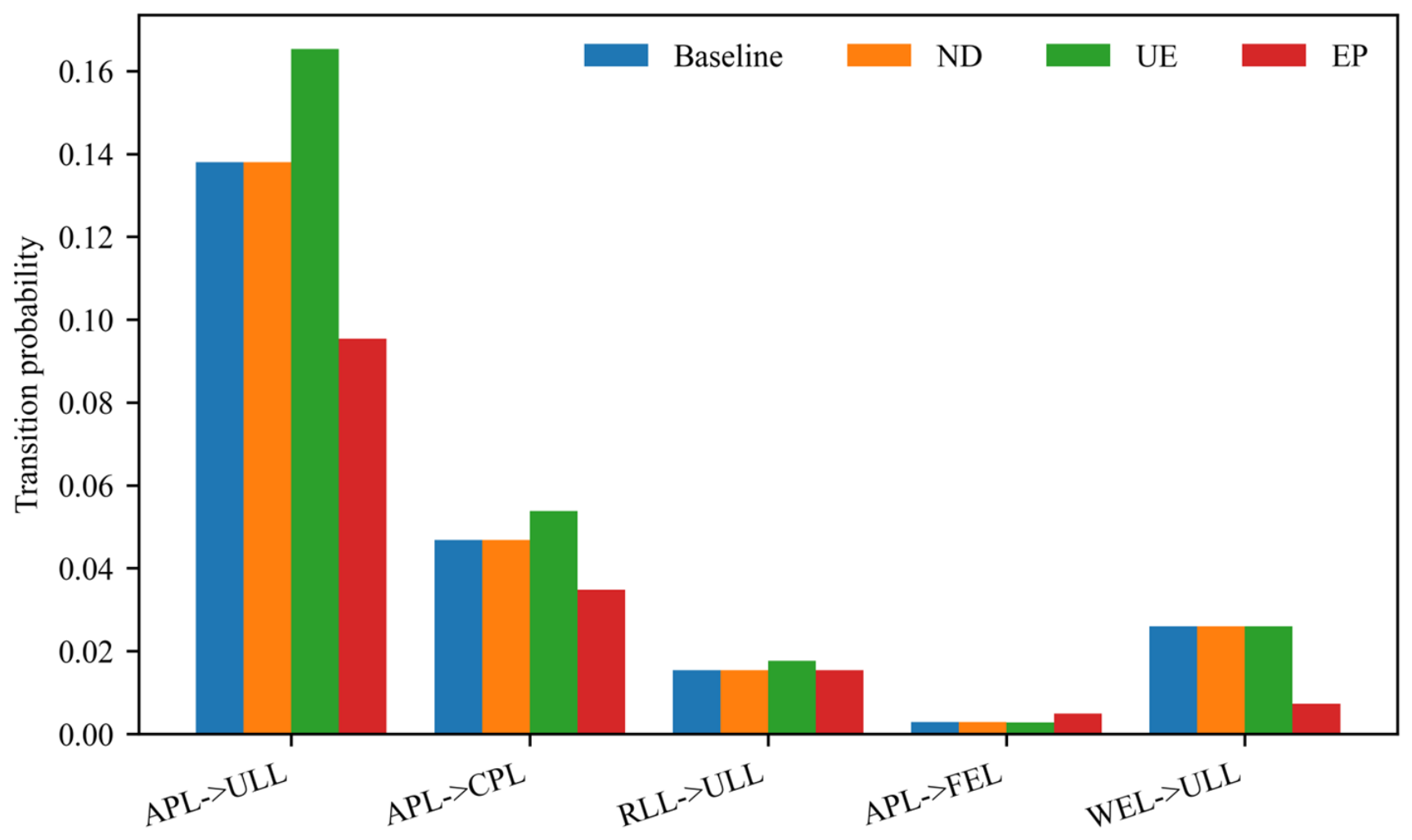
The projected land-use structure of Wenjiang District follows distinct trajectories under the three scenarios between 2030 and 2050. The urban expansion scenario intensifies the conversion of agricultural production space, the ecological protection scenario restricts transitions from ecological land, and the natural development scenario continues the historical trend. In the transition-probability adjustments shown in Figure 10, the natural development scenario retains the average historical probabilities for 2000–2025 without changing individual pathways. The urban expansion scenario used the rapid urbanization period of 2010–2015 as its reference, increasing the probabilities of APL→ULL, APL→CPL, and RLL→ULL, and decreasing those of ecological restoration pathways, such as APL→FEL and APL→GEL. The ecological protection scenario sets the transition probabilities from FEL, GEL, and WEL near zero, reduces the probabilities of APL→ULL and APL→CPL to their historical minima, and moderately increases those of APL→FEL, APL→GEL, and RLL→APL.

Figure 9. A heat map of the EC–EV–NEE coupling coordination degree ($D$) for major land-use transition pathways. NEE denotes the pathway-level contribution ${NEE}_l$, calculated using Equation (7a). $D$ represents the relative coordination of the direction-aligned and normalized EC, EV, and NEE values within the pathway sample, rather than absolute ecological performance.

Figure 9. A heat map of the EC–EV–NEE coupling coordination degree ($D$) for major land-use transition pathways. NEE denotes the pathway-level contribution ${NEE}_l$, calculated using Equation (7a). $D$ represents the relative coordination of the direction-aligned and normalized EC, EV, and NEE values within the pathway sample, rather than absolute ecological performance.

Figure 10. The transition-probability adjustments for the major land-use pathways under the baseline matrix and the natural development, urban expansion, and ecological protection scenarios.

Figure 10. The transition-probability adjustments for the major land-use pathways under the baseline matrix and the natural development, urban expansion, and ecological protection scenarios.

The CA–Markov projections show clear spatial differences among the three scenarios in 2030 and 2050 (Supplementary Figure S4). Under the urban expansion scenario, ULL and CPL continue to spread outward from the central and southeastern parts of the district, while APL contracts further. Under the ecological protection scenario, transitions from ecological land are effectively restricted, and local transitions from APL to ecological land become evident. Under the natural development scenario, the land-use pattern continues the trajectory observed between 2000 and 2025, with the magnitude of change remaining between those of the urban expansion and ecological protection scenarios. The CA–Markov backcasting results are reported in Supplementary Table S6. A five-year baseline transition probability matrix was calculated from the land-use data for 2000, 2005, and 2010. Using the 2010 PLES functional land-use map as the initial state, the model was run for one, two, and three steps to simulate the patterns observed in 2015, 2020, and 2025, respectively. The simulations yielded a Kappa coefficient of 0.82, an FoM of 0.36, and an overall area R² of 0.94. User’s accuracy ranged from 0.76 to 0.91 across the eight functional land-use classes, while producer’s accuracy ranged from 0.72 to 0.89. These metrics indicate that the model reproduced the overall historical pattern and captured part of the observed change. The subsequent scenario outputs are, therefore, used to compare relative differences under specified historical trends and scenario constraints rather than interpreted as deterministic forecasts.

3.3.2. Scenario-Specific Eco-Environmental Effects of PLES Functional Land-Use Change

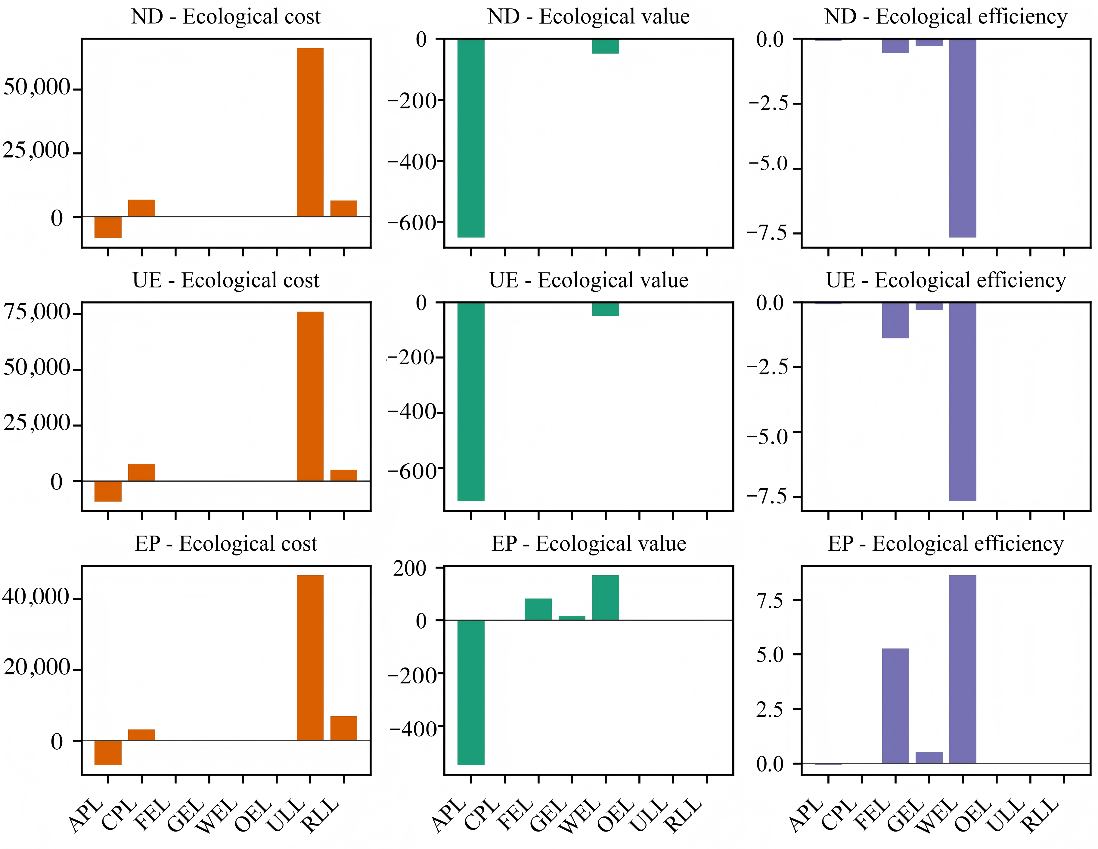
From 2030 to 2050, EC, EV, and NEE follow distinct trajectories under the three scenarios. The urban expansion scenario intensified ecological degradation, the ecological protection scenario slowed but did not fully reverse the degradation trend, and the natural development scenario produced intermediate outcomes.

APL had the highest EC, particularly under the urban expansion scenario (Figure 11). Its projected EC approached 8500 weighted ecological cost units in 2030 and remained approximately 6500 in 2050, substantially exceeding the corresponding values under the natural development and ecological protection scenarios. The EC associated with ULL was also relatively high and declined only slowly. Under the ecological protection scenario, the EC values associated with APL and ULL were substantially lower, indicating that ecological constraints reduced disturbance from land development.

EV changes remained negative under all three scenarios (Figure 11). Under the urban expansion scenario, APL experienced the greatest EV loss, while CPL and ULL also showed persistent negative changes. Under the ecological protection scenario, changes were smaller across the functional land-use classes, and FEL, GEL, and WEL remained relatively stable. Aggregate EV nevertheless remained negative, indicating that ecological pressure in Wenjiang District would persist even under ecological protection. This scenario could slow degradation but was insufficient to fully restore the ecosystem.

NEE was generally highest under the ecological protection scenario, followed by the natural development scenario, and lowest under the urban expansion scenario (Figure 11). NEE for APL continued to decline under urban expansion, whereas FEL reached its highest NEE under ecological protection. Sensitivity to the scenarios also varied among functional land-use classes. APL showed the greatest variation, followed by ULL. FEL, GEL, and WEL varied less, although their potential gains from ecological recovery remained limited. The projected areas of the principal functional land-use classes under the three scenarios are shown in Supplementary Figure S4.

3.3.3. Identification of Critical PLES Functional Land-Use Regulation Pathways

The major land-use transition pathways in Wenjiang District are classified into priority control, priority incentive, and conditional management categories by jointly considering the raw EC, EV, and NEE values, the relative coordination represented by $D$, and the responses under the three scenarios (

Table 5. Classification of major land-use transition pathways and corresponding management strategies.

Pathway Category	Representative Pathways	$\mathit{D}$ Value	Change in EC	Change in EV	NEE	Scenario Response	Management Strategy
Priority control	APL→ULL	0.191 (severe imbalance)	25433.01 (highest)	−223.25 (greatest loss)	−0.00878 (low)	Amplified under urban expansion	Restrict expansion
Priority incentive	APL→FEL, APL→GEL, APL→WEL, RLL→APL	0.870–0.968 (good coordination)	−2642 to −36 (negative; cost relief)	1.74–41.74 (gain)	0.047–0.385 (high)	Enhanced under ecological protection	Promote transitions
Conditional management	APL→CPL, APL→RLL	0.724 to 0.741 (moderate relative coordination)	6734.50 to 8625.51 (increase)	−106.41 to −75.71 (loss)	−0.01580 to −0.00878 (negative)	Relatively limited differences among scenarios	Conditional approval, intensity control, and post-implementation assessment

Note: $D$ denotes the coupling coordination degree. EC and EV denote the changes in ecological cost and ecological value associated with a pathway, respectively. NEE denotes the pathway-level contribution to network ecological efficiency, ${NEE}_l$, calculated using Equation (7a). $D$ represents the relative coordination of the three direction-aligned and normalized indicators within the pathway sample rather than absolute ecological performance. Pathway categories are determined jointly from the raw EC, EV, and NEE values, $D$, and the scenario responses. The data are obtained from Supplementary Table S4.

). APL is the functional land-use class most sensitive to scenario changes and is, therefore, the principal focus of critical pathway management. $D$ is not used as the sole basis for the management classification.

APL→ULL was identified as the priority-control pathway. It had the lowest $D$ value, at 0.191, and is classified as severely imbalanced. It also had the highest EC (25,433.01) and the greatest EV loss (−223.25). Both effects intensify under the urban expansion scenario. APL→ULL was the only pathway within an imbalance category during the study period, and its net transition area reached 28.26 km², substantially exceeding that of all other pathways. It therefore represents the principal pathway through which agricultural production space is converted to urban land in Wenjiang.

The priority-incentive pathways comprise APL→FEL, APL→GEL, APL→WEL, and RLL→APL. Their $D$ values ranged from 0.870 to 0.968, placing them within the good-coordination category. Their EV gains ranged from 1.74 to 41.74, and their transition probabilities increased under the ecological protection scenario. These pathways also attained the highest NEE values and, therefore, represent priority directions for ecological restoration and land consolidation. RLL→APL corresponds to rural land consolidation and reclamation, while APL→FEL, APL→GEL, and APL→WEL represent the restoration of ecological land from APL.

The conditional management pathways comprise APL→CPL and APL→RLL. Their $D$ values were 0.741 and 0.724, respectively, indicating moderate relative coordination. However, both pathways had positive raw EC values and negative EV and NEE values, showing that their ecological effects remain unfavorable. Their transition magnitudes and adverse effects were generally smaller than those of APL→ULL, and their changes were relatively limited across the three scenarios. They are, therefore, not placed in the same priority control category as APL→ULL. Conditional approval, constraints on development intensity, and post-implementation ecological performance assessment are recommended for these pathways.

4. Discussion

4.1. Main Findings and Interpretation

The core scientific question addressed in this study is how EC, EV, and ecological efficiency exhibit coupling characteristics across different land-use transition pathways in peri-urban transition areas, and how these coupling relationships influence the direction of regional ecological environmental quality evolution. Based on empirical analysis of Wenjiang District during 2000–2025 and scenario simulations for 2030–2050, the results indicate that the decline in ecological environmental quality in peri-urban transition areas is not determined solely by changes in the area of individual land-use types. Instead, it is driven by the imbalanced coupling of a limited number of critical transition pathways, while most pathways have already achieved moderate or good coordination.

The severe imbalance of APL→ULL ($D$ = 0.191) results from the extreme combination of resistance, value, and transition area. The ULL has the highest ecological resistance coefficient of 1000. Combined with the largest transition area from APL to ULL (28.26 km²), this pathway produces an EC of 25,433.01. Meanwhile, the ULL has an EV equivalent of 0, and the conversion of APL produces an EV loss of −223.25. Because ecological value declines along APL→ULL, its NEE, calculated as ${NEE}_l$ using Equation (7a), is −0.00878, indicating an ecological value loss along this pathway. Among these factors, the amplification effect of the transition area (28.26 km²) is most prominent, which is approximately three times that of APL→CPL (9.58 km²), resulting in an EC that is also about three times higher than that of APL→CPL (25,433.01 vs. 8625.51). This finding indicates that the imbalance of APL→ULL is not caused by a single factor, but rather results from the combined amplification effects of high resistance, low EV, and large transition area. The value of $D$ = 0.741 because APL→CPL is not inconsistent with its unfavorable raw ecological effects. Its raw EC, EV, and NEE values are 8625.51, −75.71, and −0.00878, respectively, indicating an increase in ecological cost, a loss of ecological value, and a negative pathway contribution. After direction alignment and normalization to the interval from 0.01 to 1.00, EC′, EV′, and NEE′ are 0.6027, 0.5612, and 0.4901, respectively. The similarity among these relative scores produces $C$ = 0.996. Their mean level is $T$ = 0.551, which results in $D$ = 0.741. By comparison, $EC\prime$ and $EV\prime$ for APL→ULL are both close to 0.01, whereas $NEE\prime$ is approximately 0.490. The greater disparity among these scores reduces $C$ and $D$ to 0.215 and 0.191, respectively. Moderate relative coordination for APL→CPL, therefore, describes the arithmetic balance of the direction-aligned indicators within the pathway sample. It does not indicate a low absolute ecological cost, a positive ecological value, or a sustainable ecological outcome. The pathway remains subject to conditional management because its raw ecological effects are unfavorable. The good coordination of APL→FEL, APL→GEL, and APL→WEL ($D$ = 0.870–0.968) benefits from the low resistance coefficients (5–22) and high EV equivalents (11.67–45.35) of forest land, grassland, and water ecological land. The flower and nursery industry in Wenjiang District also helps maintain the ecological functions of FEL to some extent and provides a buffer against the pressure of urban expansion [38]. The good coordination of RLL→APL ($D$ = 0.897) corresponds to a pattern characterized by negative costs and positive value gains associated with rural spatial improvement and land reclamation.

At the stage level, the single land-use dynamic degree of ULL reached 11.684% from 2000 to 2005, while that of CPL reached 24.641% from 2010 to 2015. Both periods also had relatively high comprehensive land-use dynamic degrees, and the ECR was lowest from 2010 to 2015. A study conducted at the Chengdu metropolitan scale likewise documented continued cropland occupation by urban expansion and identified Wenjiang as one of the more strongly affected districts [42]. However, this study did not test the causal effects of specific spatial policies, industrial agglomeration, or the concentration of educational resources. These stage-specific changes are, therefore, interpreted as temporal associations consistent with urban expansion and functional concentration, rather than as effects caused by a particular policy or industry. The scenario simulations show that EV still exhibits a negative change under the ecological protection scenario, suggesting that this scenario can mitigate but cannot completely reverse the existing degradation trend. This occurs because the ecological spatial base in Wenjiang District is relatively limited, and the transition area of restoration-oriented pathways such as APL→FEL (0.59 km²) is much smaller than that of APL→ULL (28.26 km²). Consequently, the accumulated pressure from historical urbanization generates a strong inertia that cannot be fully eliminated under scenario constraints.

4.2. Methodological Contribution and the Boundaries of Originality in the Pathway Coupling Framework

Previous studies have provided a direct methodological basis for each component of the framework. Research on the eco-environmental effects of PLES commonly combines transition matrices with the EQI, ECR, or ESV to examine changes in land-use structure and aggregate ecological responses [13,14,15,16]. Complex network methods have been used to identify the topology and critical nodes of land-use transitions [17,18,19,20]. Xu et al. [27] incorporated EC and EV into NEE for land-use transition networks to assess network functional vulnerability. Building on this network concept, the present study defines the ratio associated with each directed transition edge as the pathway-level contribution ${\mathrm{N}\mathrm{E}\mathrm{E}}_{\mathrm{l}}$ and uses ${\mathrm{N}\mathrm{E}\mathrm{E}}_{\mathrm{n}\mathrm{e}\mathrm{t}}$ for the overall network indicator obtained by aggregating pathway contributions. Coupling coordination models have been used to compare relative coordination in multi-indicator systems [28,29]. CA–Markov and other model chains have been applied to land-use scenario simulation and PLES conflict prediction [30,31,32,33,34]. This study retains the basic concepts and application boundaries of the component methods while applying the pathway-scale operationalization and notation of NEE described above. Its additional contribution remains the use of a common analytical unit and the linkage of successive analytical stages. ${\mathrm{N}\mathrm{E}\mathrm{E}}_{\mathrm{l}}$ is not presented as a newly proposed general efficiency indicator.

First, this study uses each specific $i$→$j$ land-use transition pathway as a common unit of analysis. The transition matrix records pathway direction and magnitude, while the complex network identifies the pathways’ network position. EC, EV, and NEE, with NEE calculated as ${\mathrm{N}\mathrm{E}\mathrm{E}}_{\mathrm{l}}$ using Equation (7a), describe pathway-level changes in cost, changes in value, and efficiency contributions, respectively. $D$ compares the relative coordination of these three dimensions within the same evaluation set. This structure establishes a direct correspondence among pathway magnitude, network position, and ecological performance. For example, both APL→ULL and APL→CPL lead to classes with high ecological resistance, but the two pathways differ in EC, EV, NEE, and $D$ because their transition magnitudes and indicator profiles differ. Aggregate indices such as the EQI and ECR, or any single ecological indicator, cannot independently provide this pathway-level correspondence. Here, $D$ represents only relative coordination. It is not a measure of absolute ecological benefit and does not demonstrate causal synergy among the indicators [28].

Second, the same set of pathway identifiers links historical diagnosis with future scenario comparisons. The historical analysis uses network structure together with EC, EV, NEE, and $D$ to identify the major pathways. The three scenarios then adjust the transition probabilities of APL→ULL, APL→CPL, RLL→ULL, and ecological restoration pathways to compare the responses of these pathways under different development constraints. Compared with integrated model chains that primarily output land-use patterns or spatial conflict intensity [34], this study retains individual transition pathways as the connecting units for historical analysis, scenario design, and management classification. The Methods Section also report the scenario multipliers and the procedure used to normalize each row. Backcasting yields a Kappa value of 0.82, an FoM of 0.36, and an overall area R² of 0.94. These details document the scenario construction process and the model’s ability to reproduce the aggregate pattern and part of the observed change. They are not presented as an independent claim of originality.

Third, the pathway diagnosis is translated into a management classification. The classification considers the ecological performance represented by EC, EV, and NEE, the relative coordination represented by $D$, and the responses under different scenarios. It is not determined by any single indicator or by $D$ alone. This process produces priority-control, priority-incentive, and conditional-management pathways. Unlike uniform measures based on the total areas of land-use classes or aggregate eco-environmental quality, these categories correspond to specific transition directions such as APL→ULL, APL→FEL, and APL→CPL. The methodological contribution, therefore, lies in extending the analytical scale and linking the analytical stages. Apart from the pathway-scale operationalization and notation of NEE, the basic concepts and application boundaries of the component indicators and models remain unchanged.

4.3. The Representativeness of the Findings for Peri-Urban Transition Zones

To assess the range of settings to which the Wenjiang findings may apply, this study compares Wenjiang with PLES studies of Suzhou City, Shizhu County in Chongqing, and Datong County in Qinghai Province (

Table 6. Structured comparison of PLES transitions and ecological responses across contrasting regional contexts.

Region	Regional Context	Study Period	Verified PLES Transition Pattern	Ecological Response Reported in the Original Study	Joint Pathway-Level Analysis of EC, EV, and NEE
Wenjiang District	Peri-urban plain district adjacent to a megacity	2000 to 2025	APL→ULL was dominant. APL→CPL and RLL→APL were also major pathways.	EQI decreased from 0.228 to 0.200. APL→ULL had the highest EC and the greatest EV loss.	Quantified in this study
Suzhou City [50]	Rapidly urbanizing city	1980 to 2018	Production land decreased, ecological land increased slightly, and living land increased rapidly.	EQI decreased from 0.4312 to 0.4139.	Not reported in the cited study
Shizhu County, Chongqing [51]	Mountainous county in the Three Gorges Reservoir Area	1990 to 2020, with a scenario for 2035	Production space decreased slightly, ecological space increased slightly, and living space increased markedly.	Ecological space accounted for more than 65%. The ecological protection scenario maintained the ecological space pattern and increased its area.	Not reported in the cited study
Datong County, Qinghai Province [52]	Ecologically fragile plateau county	2010 to 2018	Living-production land became more concentrated and occupied parts of ecological-production land and production-ecological land.	The cited study did not report a directly comparable EQI.	Not reported in the cited study

Note. The values and trends in this table are taken from the classification systems and assessment methods used in the respective studies. Differences in the functional space classification, indicator construction and weighting, spatial scale, study period, and ecological response variables preclude direct comparison of the magnitude or rate of ecological change. Therefore, these results are only used for comparing transition directions and analytical dimensions, rather than for ranking the ecological change magnitude and rate across different regions. “Not reported” refers only to the corresponding study cited in this table.

). The three comparison cases cover a rapidly urbanizing city, a mountainous county in the Three Gorges Reservoir Area, and an ecologically fragile plateau county. The comparison focuses on transition directions and analytical dimensions. It does not rank the magnitude of index changes reported under different evaluation systems.

Wenjiang and Suzhou both experienced a contraction of production space, an expansion of living or construction space, and an overall decline in eco-environmental quality. The EQI decreased from 0.228 to 0.200 in Wenjiang and from 0.4312 to 0.4139 in Suzhou [50]. These values describe temporal change within each evaluation system and are not directly comparable because the studies differ in functional space classification, ecological quality weights, spatial scale, and study period. In Shizhu County, production space decreased slightly, ecological space increased slightly, and living space increased markedly from 1990 to 2020. Under the ecological protection scenario, the ecological space pattern was maintained, and its area increased [51]. In Datong County, Qinghai Province, living-production land became more concentrated from 2010 to 2018 and occupied parts of ecological-production land and production-ecological land [52]. These differences show that PLES transitions depend on regional context. The magnitude and mechanism of an ecological response observed in one case cannot be directly extrapolated to another.

The main contribution of the Wenjiang analysis lies not in demonstrating that Wenjiang has the largest decline in eco-environmental quality, but in the decomposition of aggregate spatial change into specific transition pathways, followed by a joint assessment of EC, EV, and NEE for each pathway within a consistent evaluation system. The comparison studies in Table 6 did not report a joint pathway-level analysis of these three indicators. The Wenjiang findings could inform pathway-based management in peri-urban plain areas adjacent to megacities that face similar urban expansion pressures and have comparable spatial structures. They should not be interpreted as a universal pattern for all peri-urban transition zones.

4.4. The Reliability and Uncertainty of the Findings

This study assessed the reliability of the main findings through weight sensitivity analysis, temporal comparison of network structure, and CA–Markov backcasting validation. These assessments address evaluation parameters, historical transition structure, and spatial projection, respectively, but they do not remove the associated uncertainties. The sources of uncertainty in the expert-derived weights and future scenario projections, therefore, need to be considered separately, together with the limits of the conclusions supported by each assessment.

The weights assigned to the eight functional land-use classes in the EQI were obtained from the AHP judgment matrix. The consistency ratio was 0.046, indicating that the matrix met the internal consistency requirement [44]. However, a consistency test cannot remove subjectivity arising from the composition of the expert group, interpretation of the pairwise comparison scale, or regional experience. The EQI declined from 2000 to 2025 under all 32 one-at-a-time perturbation settings of ±10% and ±20%. The cumulative decline ranged from 10.1% to 13.5%, compared with the baseline decline of 12.3%. In the Monte Carlo results, the interquartile ranges and baseline estimates shifted downward over time, but the 95% simulation intervals for adjacent years overlapped. Figure 8 shows that the APL weight had the largest effect on the EQI in 2025. These results show that the long-term downward trend was robust to the specified weight perturbations. They do not show that the absolute EQI values or the declines between adjacent years are independent of the selected weights, nor do the simulation intervals alone establish statistically significant differences between adjacent years.

The comparison between the two historical periods provides another line of evidence. The network for 2000 to 2010 contained six nodes and five edges, had a density of 0.167, and identified APL as the hub node. The network for 2010 to 2025 contained seven nodes and 31 edges, had a density of 0.738, and identified ULL and RLL as the hub nodes. Transitions between APL and living space remained important in both periods, supporting the persistence of the main transition direction. At the same time, changes in the number of edges, network density, and hub nodes show that the network shifted from concentration in a few pathways to the coexistence of multiple pathways. The historical structure should, therefore, not be regarded as fully stationary.

Backcasting validation of the CA–Markov model yielded a Kappa coefficient of 0.82, indicating high overall agreement between the simulated and observed maps. Because Kappa can combine quantity disagreement with spatial allocation disagreement, model performance was not classified using Kappa alone. Kappa was considered together with an FoM of 0.36, an overall area R² of 0.94, and the user’s and producer’s accuracies for each land-use class [48,49]. These metrics indicate that the model reproduces the overall historical pattern and captures part of the observed transitions. Backcasting nevertheless evaluates reproduction of historical data; it does not provide probability intervals for the 2030 and 2050 scenario outputs. Future scenarios remain sensitive to the baseline transition probabilities and scenario multipliers, the CA–Markov structure and spatial allocation rules, errors in the 30 m input data, and external changes in policy and infrastructure [41,53]. These uncertainties are more likely to accumulate over a longer projection horizon, so the 2050 results require more cautious interpretation than the 2030 results. EC, EV, and NEE are calculated from the simulated land-use transitions and, therefore, inherit uncertainty from the scenario patterns and coefficient assumptions. The scenario outputs are interpreted as plausible states under the specified historical trends, neighborhood rules, and development constraints. Their management implications rely mainly on relative differences and directions of change across scenarios, rather than on exact point predictions.

4.5. Policy Implications

The pathway coupling analysis in this study (

Table 7. Differentiated policy instrument matrix based on coupling types.

Pathway Type	Representative Pathways	$\mathit{D}$ Range	Spatial Regulation	Economic Incentives	Performance Evaluation	Technical Guidance
Priority-control type	APL→ULL	0.191 (severe imbalance)	Strict constraints	Strict ecological compensation requirements	Pre-project assessment	Prioritize redevelopment of existing land
Priority-incentive type	APL→FEL, APL→GEL, APL→WEL, RLL→APL	0.870–0.968 (good coordination)	Maintain spatial continuity	Ecological compensation and land consolidation incentives	Benefit tracking	Ecological restoration oriented
Conditional management type	APL→CPL, APL→RLL	0.724 to 0.741 (moderate relative coordination)	Conditional approval and intensity control	Differentiated compensation	Post-implementation assessment	Low-impact development

Note: D represents the relative coordination of the direction-aligned and normalized EC, EV, and NEE values within the pathway sample. The policy categories are determined jointly from the raw EC, EV, and NEE values, D, and the scenario responses. D is not used as the sole classification criterion.

) shows that the coupling coordination degree of EC, EV, and NEE among different land-use transition pathways exhibits a hierarchical differentiation from severe imbalance to good coordination. This finding indicates that ecological regulation in peri-urban transition areas needs to shift from overall land-use quantity control to pathway-based classification management. This finding complements existing PLES studies by addressing the insufficient quantitative analysis of coupling relationships at the transition pathway level [17,18,53]. The APL→ULL pathway represents a severely imbalanced pathway ($D$ = 0.191). The combined pattern of high EC (25,433.01), high value loss (−223.25), and low NEE (−0.00878) indicates that this pathway is the primary driver of ecological degradation in Wenjiang District. Combined with the simulation results showing a further increase in EC under the urban expansion scenario, this pathway is identified as a priority target for management measures, including construction land increment control, permanent basic farmland protection, and project access assessment. The APL→FEL, APL→GEL, APL→WEL, and RLL→APL pathways represent well-coordinated pathways ($D$ = 0.870–0.968). Their matching relationship between negative EC and positive EV gains indicates that these pathways should be prioritized for ecological restoration and land improvement. Specifically, RLL→APL corresponds to rural spatial improvement, whereas APL→FEL/GEL/WEL represents the restoration of APL to ecological land. These pathways can be promoted through incentive mechanisms, such as ecological compensation, land improvement, and green infrastructure development [5,39,54]. APL→CPL and APL→RLL are classified as conditional management pathways. Their D values range from 0.724 to 0.741, indicating moderate relative coordination. However, their EC values are 8625.51 and 6734.50, their EV values are −75.71 and −106.41, and both pathways have negative NEE values. This relative coordination level should, therefore, not be interpreted as evidence of minor ecological effects or favorable ecological performance. Compared with APL→ULL, these two pathways generally have smaller transition magnitudes and adverse effects, together with relatively limited scenario responses. Conditional approval, development intensity control, and post-implementation assessment are therefore more appropriate than the measures applied to priority control pathways. Management decisions should be based on the combined evidence from raw ecological effects, relative coordination, and scenario responses rather than on $D$ alone.

4.6. Limitations and Future Research

This study has four limitations. First, the 30 m CNLUCC data are suitable for land-use pattern analysis at district and county scales, but mixed pixels may occur along narrow rivers and canals, road edges, and highly fragmented patches. Changes in ecological land at fine spatial scales may, therefore, be underestimated. Second, the EQI is calculated from the eco-environmental quality weights assigned to the functional land-use classes rather than from direct observations of biophysical variables, such as NDVI, NPP, or biodiversity. The AHP consistency test and weight sensitivity analysis indicate that the long-term downward direction is relatively stable, but they cannot remove the influence of expert judgment and weight specification on the absolute EQI values. Third, CA–Markov assumes some persistence in historical transition probabilities and neighborhood relationships. Scenario multipliers, spatial allocation rules, input data errors, policy adjustments, major infrastructure development, and changes in industrial layout may cause future patterns to depart from the scenario outputs [41,55]. These uncertainties may accumulate as the projection horizon increases. The results for 2030 and 2050, therefore, represent plausible states under specified assumptions and constraints rather than deterministic predictions. Fourth, $D$ is a relative indicator calculated after direction alignment and normalization using the minimum and maximum values of the 31 pathways examined in this study. It is, therefore, sensitive to the sample range and extreme values and should not be used to assess absolute ecological performance outside this pathway set or to support uncalibrated cross-regional comparisons. In addition, ${NEE}_l$ is derived from EC and EV, so the three indicators are not fully independent. $D$ is consequently used as a descriptive joint diagnostic within the pathway sample rather than as evidence of causal coupling among EC, EV, and NEE. The value of $D$ = 0.741 for APL→CPL reflects the relative balance of its three normalized scores and does not offset the increase in raw ecological cost or the loss of ecological value. Future research could use independent ecological observations to examine the stability of the pathway classification and evaluate the sensitivity of $D$ and its categories to alternative normalization ranges and weighting schemes.

Future research can proceed in four directions. First, measured or remotely sensed indicators, such as NDVI, NPP, habitat quality, and ecosystem services, can be used to validate the EQI independently and strengthen the biophysical basis of the eco-environmental quality assessment. Second, independent expert groups, alternative weights, or combined subjective and objective weighting schemes can be used to report the dispersion of the EQI results across weight specifications. Scenario ensembles containing multiple transition probability settings, scenario multipliers, and alternative models can also be constructed to quantify the uncertainty ranges of the 2030 and 2050 outputs [41,55]. Third, the pathway coupling framework can be applied to other peri-urban districts of Chengdu, including Pidu, Shuangliu, and Longquanyi, and extended to the Chengdu Plain Urban Agglomeration and the Chengdu–Chongqing Economic Circle to test its robustness and transferability across spatial scales and peri-urban transition zones. Fourth, further research can examine how transition magnitude, indicator synchrony, spatial neighborhood effects, and related factors influence coupling coordination among land-use transitions with the same resistance coefficient, including the coordination observed for APL→CPL.

5. Conclusions

This study develops a pathway-coupling analytical framework that integrates complex network theory, a coupling coordination degree model, and CA–Markov scenario simulation. The framework examines how the ecological cost–value–efficiency coupling characteristics of different land-use transition pathways influence the direction of eco-environmental quality change in a peri-urban transition zone.

The decline in eco-environmental quality in Wenjiang is associated with the concentration of unfavorable ecological effects along a small number of critical transition pathways rather than with the simple accumulation of area changes among land-use classes. From 2000 to 2025, the reconfiguration of PLES is dominated by APL→ULL, with a transition area of 28.26 km². The land-use transition network expands from 5 to 31 edges, and network density increases from 0.167 to 0.738, indicating a shift from concentrated transitions toward the coexistence of multiple pathways. The EQI decreases continuously from 0.228 to 0.200, representing a cumulative decline of approximately 12.3%. The ECR remains negative in every period, with the strongest degradation occurring during 2000–2005, when the ECR reaches −0.01060, and 17.388 km² of APL is converted. $D$ varies from severe imbalance to good relative coordination across the pathways. APL→ULL has the lowest $D$ at 0.191. APL→CPL shows moderate relative coordination with $D$ = 0.741, while APL→FEL and related pathways show good relative coordination with $D$ values ranging from 0.870 to 0.968. Most pathways achieve moderate or good coordination. The three scenario simulations show that ecological protection can slow but cannot completely reverse the decline in EV, and APL is the land-use class most sensitive to changes across scenarios. Based jointly on the raw ecological effects, relative coordination, and scenario responses, the major transition pathways are classified into priority control, priority incentive, and conditional management categories. APL is the principal land-use class for identifying and managing critical transition pathways.

These findings indicate that ecological governance in peri-urban transition zones should move from aggregate control of land-use classes toward differentiated pathway management. Strict constraints, ecological compensation and incentives, and conditional approval should be applied to priority control, priority incentive, and conditional management pathways, respectively. This study remains subject to limitations arising from the 30 m data resolution, the expert-derived EQI weights, and the CA–Markov assumption that historical transition relationships persist. The results for 2030 and 2050 should be interpreted as plausible states under specified transition probabilities, neighborhood rules, and scenario constraints. The management recommendations rely mainly on relative differences and directions of change across scenarios rather than on exact point predictions. Future research could incorporate biophysical indicators, such as NDVI and NPP, compare results under alternative weighting schemes and multimodel scenario ensembles, and test the framework across spatial scales in other peri-urban districts of Chengdu, including Pidu and Shuangliu, and in the Chengdu–Chongqing Economic Circle.

References

1. Lambin, E.F.; Meyfroidt, P. Global land use change, economic globalization, and the looming land scarcity. Proc. Natl. Acad. Sci. USA 2011, 108, 3465–3472. [Google Scholar] [CrossRef] [Scilit]
2. Turner, B.L., II; Lambin, E.F.; Reenberg, A. The emergence of land change science for global environmental change and sustainability. Proc. Natl. Acad. Sci. USA 2007, 104, 20666–20671. [Google Scholar] [CrossRef] [Scilit]
3. Newbold, T.; Hudson, L.N.; Hill, S.L.L.; Contu, S.; Lysenko, I.; Senior, R.A.; Börger, L.; Bennett, D.J.; Choimes, A.; Collen, B.; et al. Global effects of land use on local terrestrial biodiversity. Nature 2015, 520, 45–50. [Google Scholar] [CrossRef] [Scilit]
4. Qin, C.Y.; Pang, Z.H.; Li, K.; Liu, Z.Y.; Yan, D.M.; Xiang, K.N.; He, J.P.; Zhou, J.; Ye, Y.Y.; Zeng, K.; et al. Coupled effects of land-use/cover change and climate change on ecosystem services from a cross-scale perspective: Research progress and future directions. Ecol. Front. 2026; in press. [CrossRef] [Scilit]
5. Foley, J.A.; DeFries, R.; Asner, G.P.; Barford, C.; Bonan, G.; Carpenter, S.R.; Chapin, F.S.; Coe, M.T.; Daily, G.C.; Gibbs, H.K.; et al. Global consequences of land use. Science 2005, 309, 570–574. [Google Scholar] [CrossRef] [Scilit]
6. Cui, X.; Xu, N.; Chen, W.; Wang, G.; Liang, J.; Pan, S.; Duan, B. Spatio-temporal variation and influencing factors of the coupling coordination degree of production-living-ecological space in China. Int. J. Environ. Res. Public Health 2022, 19, 10370. [Google Scholar] [CrossRef] [Scilit]
7. Zhou, D.; Xu, J.; Lin, Z. Conflict or coordination? Assessing land use multi-functionalization using production-living-ecology analysis. Sci. Total Environ. 2017, 577, 136–147. [Google Scholar] [CrossRef] [Scilit]
8. Bu, Z.; Fu, J.; Jiang, D.; Lin, G. Production-living-ecological spatial function identification and pattern analysis based on multi-source geographic data and machine learning. Land 2023, 12, 2029. [Google Scholar] [CrossRef] [Scilit]
9. Spyra, M.; La Rosa, D.; Zasada, I.; Sylla, M.; Shkaruba, A. Governance of ecosystem services trade-offs in peri-urban landscapes. Land Use Policy 2020, 95, 104617. [Google Scholar] [CrossRef] [Scilit]
10. Salem, M.; Ravetz, J.; Sareen, S.; Dong, T.; Haque, M.; Bayoumi, W.; Tsurusaki, N.; Xu, G. Managing the urban-rural transition: A review of approaches and policies for peri-urban land use. J. Urban Manag. 2025, 14, 1115–1129. [Google Scholar] [CrossRef] [Scilit]
11. Ma, W.; Yang, H.; Jiang, G.; Zhou, T.; Zhao, Q. Exploring trade-offs between residential and industrial functions in rural areas and their ecological impacts across transitioning agricultural systems: Evidence from the metropolitan suburbs of China. J. Environ. Manag. 2024, 358, 120907. [Google Scholar] [CrossRef] [Scilit]
12. Li, Y.; Tang, Y.; Ives, C.D. Policy-driven scenarios for sustainable peri-urban land use: Production-living-ecological space in Yubei District, Chongqing. Land 2025, 14, 1074. [Google Scholar] [CrossRef] [Scilit]
13. Ren, L.; Wang, X.; Jiang, W.; Ren, M.; Yin, L.; Zhang, X.; Zhang, B. Exploring impact and driving forces of land use transformation on ecological environment in urban agglomeration from the perspective of production-living-ecological spatial synergy. Sustainability 2025, 17, 8235. [Google Scholar] [CrossRef] [Scilit]
14. Yi, M.; Yan, Q.; Li, K.; Ma, X.; Li, G.; Wu, Z.; Pan, Q.; Chen, X. The ecological environmental effects and topographic gradient analysis of transformation in the production-living-ecological spaces in the northern slope of the Tianshan Mountains. Land 2024, 13, 1170. [Google Scholar] [CrossRef] [Scilit]
15. Yang, Y.Y.; Bao, W.K.; Li, Y.H.; Wang, Y.S.; Chen, Z.F. Land use transition and its eco-environmental effects in the Beijing-Tianjin-Hebei urban agglomeration: A production-living-ecological perspective. Land 2020, 9, 285. [Google Scholar] [CrossRef] [Scilit]
16. Liu, Q.; Zhao, S.L.; Li, Y.F. The hidden costs of land use transformation: Ecological degradation in arid and semi-arid areas. J. Arid Environ. 2025, 230, 105433. [Google Scholar] [CrossRef] [Scilit]
17. Zhang, M.; Wang, J.; Feng, Y. Temporal and spatial change of land use in a large-scale opencast coal mine area: A complex network approach. Land Use Policy 2019, 86, 375–386. [Google Scholar] [CrossRef] [Scilit]
18. Wang, Y.; Li, X.; Li, J.; Huang, Z.; Xiao, R. Impact of rapid urbanization on vulnerability of land system from complex networks view: A methodological approach. Complexity 2018, 2018, 8561675. [Google Scholar] [CrossRef] [Scilit]
19. Wang, Z.; Li, T.; Yang, S.; Zhong, D. Spatio-temporal dynamic and structural characteristics of land use/cover change based on a complex network: A case study of the middle reaches of Yangtze River urban agglomeration. Sustainability 2022, 14, 6941. [Google Scholar] [CrossRef] [Scilit]
20. Zhang, Q.; Yan, M.; Zhang, L.; Shao, W.; Chen, Y.; Dong, Y. Three decades of oasis transition and its driving factors in Turpan-Hami Basin in Xinjiang, China: A complex network approach. Remote Sens. 2024, 16, 465. [Google Scholar] [CrossRef] [Scilit]
21. Li, F.; Ye, Y.; Song, B.; Wang, R. Evaluation of urban suitable ecological land based on the minimum cumulative resistance model: A case study from Changzhou, China. Ecol. Model. 2015, 318, 194–203. [Google Scholar] [CrossRef] [Scilit]
22. Costanza, R.; de Groot, R.; Sutton, P.; van der Ploeg, S.; Anderson, S.J.; Kubiszewski, I.; Farber, S.; Turner, R.K. Changes in the global value of ecosystem services. Glob. Environ. Change 2014, 26, 152–158. [Google Scholar] [CrossRef] [Scilit]
23. Xie, G.D.; Zhang, C.X.; Zhang, L.M.; Chen, W.H.; Li, S.M. Improvement of the evaluation method for ecosystem service value based on per unit area. J. Nat. Resour. 2015, 30, 1243–1254. [Google Scholar] [CrossRef]
24. Lindeman, R.L. The trophic-dynamic aspect of ecology. Ecology 1942, 23, 399–417. [Google Scholar] [CrossRef] [Scilit]
25. Huppes, G.; Ishikawa, M. A framework for quantified eco-efficiency analysis. J. Ind. Ecol. 2005, 9, 25–41. [Google Scholar] [CrossRef] [Scilit]
26. Latora, V.; Marchiori, M. Efficient behavior of small-world networks. Phys. Rev. Lett. 2001, 87, 198701. [Google Scholar] [CrossRef] [Scilit]
27. Xu, S.; Liu, G.; Mou, B. Vulnerability analysis of land ecosystem considering ecological cost and value: A complex network approach. Ecol. Indic. 2023, 147, 109941. [Google Scholar] [CrossRef] [Scilit]
28. Wang, S.J.; Kong, W.; Ren, L.; Zhi, D.D.; Dai, B.T. Research on misuses and modification of coupling coordination degree model in China. J. Nat. Resour. 2021, 36, 793–810. [Google Scholar] [CrossRef] [Scilit]
29. Zhang, F.; Xie, A.; Jiang, C.; Chen, J.; An, Y.; Yang, P.; Ma, D. Coupling coordination analysis and spatio-temporal heterogeneity between urban land green use efficiency and ecosystem services in Yangtze River Economic Belt, China. Humanit. Soc. Sci. Commun. 2024, 11, 1328. [Google Scholar] [CrossRef] [Scilit]
30. Luan, C.; Liu, R.; Li, Y.; Zhang, Q. Comparison of various models for multi-scenario simulation of land use/land cover to predict ecosystem service value: A case study of Harbin-Changchun Urban Agglomeration, China. J. Clean. Prod. 2024, 478, 144012. [Google Scholar] [CrossRef] [Scilit]
31. Burnham, B.O. Markov intertemporal land use simulation model. J. Agric. Appl. Econ. 1973, 5, 253–258. [Google Scholar] [CrossRef] [Scilit]
32. Subedi, P.; Subedi, K.; Thapa, B. Application of a hybrid cellular automaton-Markov model in land-use change prediction: A case study of Saddle Creek drainage basin, Florida. Appl. Ecol. Environ. Sci. 2013, 1, 126–132. [Google Scholar] [CrossRef] [Scilit]
33. Kumar, S.; Radhakrishnan, N.; Mathew, S. Land use change modelling using a Markov model and remote sensing. Geomat. Nat. Hazards Risk 2014, 5, 145–156. [Google Scholar] [CrossRef] [Scilit]
34. Xiong, S.; Yang, F.; Zhang, J.; Tang, Y. An integrated model chain for diagnosing and predicting conflicts between production-living-ecological space in lake network regions: A case of the Dongting Lake region, China. Ecol. Indic. 2024, 166, 112237. [Google Scholar] [CrossRef] [Scilit]
35. Xiong, B.; Deng, L.; Luo, G.; Pan, W.; Lao, X.; Zhu, Z.; Yin, H. Spatiotemporal evolution and driving mechanisms of the transformation of production-living-ecological land in peri-urban areas under the construction of the Guangdong-Hong Kong-Macao greater bay area: A case study of Huiyang district, China. Front. Environ. Sci. 2026, 13, 1697838. [Google Scholar] [CrossRef] [Scilit]
36. Zuo, M.; Liu, G.; Jing, C.; Zhang, R.; Wang, X.; Mao, W.; Shen, L.; Dai, K.; Wu, X. Spatiotemporal patterns and driving factors of cropland abandonment in metropolitan suburbs: A case study of Chengdu directly administered zone, Tianfu New Area, Sichuan Province, China. Land 2025, 14, 1311. [Google Scholar] [CrossRef] [Scilit]
37. Lu, Y.; He, T.; Yue, W.; Li, M.; Shan, Z.; Zhang, M. Does cropland threaten urban land use efficiency in the peri-urban area? Evidence from metropolitan areas in China. Appl. Geogr. 2023, 161, 103124. [Google Scholar] [CrossRef] [Scilit]
38. Li, W.J.; Kang, J.W.; Wang, Y. Identifying the contribution and spatial effects of land use conversion on ecosystem health in Chongqing: A multi-scenario simulation perspective. Ecol. Indic. 2024, 165, 112232. [Google Scholar] [CrossRef] [Scilit]
39. Wang, S.T.; Ge, Y.C. Ecological quality response to multi-scenario land-use changes in the Heihe River Basin. Sustainability 2022, 14, 2716. [Google Scholar] [CrossRef] [Scilit]
40. Pereira, P.; Inácio, M.; Pinto, L.; Kalinauskas, M.; Bogdzevic, K.; Zhao, W. Mapping ecosystem services in urban and peri-urban areas: A systematic review. Geogr. Sustain. 2024, 5, 491–509. [Google Scholar] [CrossRef] [Scilit]
41. Yang, Y.; Lu, Z.; Yang, M.; Yan, Y.; Wei, Y. Impact of land use changes on uncertainty in ecosystem services under different future scenarios: A case study of Zhang-Cheng area, China. J. Clean. Prod. 2024, 434, 139881. [Google Scholar] [CrossRef] [Scilit]
42. Meng, B.; Wang, X.; Zhang, Z.; Huang, P. Spatio-temporal pattern and driving force evolution of cultivated land occupied by urban expansion in the Chengdu Metropolitan Area. Land 2022, 11, 1458. [Google Scholar] [CrossRef] [Scilit]
43. Dai, X.; Li, Y.; Qi, Y.; Chen, Y.; Yan, D.; Xia, K.; He, S.; He, Y. Coupling agricultural green development and Park City development: An empirical analysis from Chengdu, China. Agriculture 2025, 15, 248. [Google Scholar] [CrossRef] [Scilit]
44. Saaty, T.L. Decision making with the analytic hierarchy process. Int. J. Serv. Sci. 2008, 1, 83–98. [Google Scholar] [CrossRef] [Scilit]
45. Li, P.; Gao, J.; Chen, J. Quantitative assessment of ecological stress of construction lands by quantity and location: Case study in Southern Jiangsu, Eastern China. Environ. Dev. Sustain. 2020, 22, 1559–1578. [Google Scholar] [CrossRef] [Scilit]
46. Adriaensen, F.; Chardon, J.P.; De Blust, G.; Swinnen, E.; Villalba, S.; Gulinck, H.; Matthysen, E. The application of least-cost modelling as a functional landscape model. Landsc. Urban Plan. 2003, 64, 233–247. [Google Scholar] [CrossRef] [Scilit]
47. Rina, S.; Bole, Y.; Tong, Z.; Zhi, F.; Xu, J.; Ma, B.; Liu, X.; Zhang, J. Ecological zoning study on the coupling of land use intensity and landscape ecological risk in Western Jilin: A production-living-ecological space perspective. Sustainability 2024, 16, 10992. [Google Scholar] [CrossRef] [Scilit]
48. Varga, O.G.; Pontius, R.G., Jr.; Singh, S.K.; Szabó, S. Intensity analysis and the Figure of Merit’s components for assessment of a Cellular Automata-Markov simulation model. Ecol. Indic. 2019, 101, 933–942. [Google Scholar] [CrossRef] [Scilit]
49. Pontius, R.G., Jr.; Millones, M. Death to Kappa: Birth of quantity disagreement and allocation disagreement for accuracy assessment. Int. J. Remote Sens. 2011, 32, 4407–4429. [Google Scholar] [CrossRef] [Scilit]
50. Ben, X.C.; Yu, C. Ecological effects of land use transformation and its driving force based on production-living-ecological space: A case study of Suzhou City. J. Environ. Eng. Technol. 2022, 12, 1428–1436. [Google Scholar] [CrossRef]
51. Chen, H.J.; Yang, Q.Y.; Peng, L.X.; Su, K.C.; Zhang, H.Z.; Liu, X.Y. Spatiotemporal evolution characteristics and scenario simulation of production-living-ecological space at county level in Three Gorges reservoir are-as. Trans. Chin. Soc. Agric. Eng. 2022, 38, 285–294. [Google Scholar] [CrossRef]
52. Cheng, X.D.; Qu, L.P.; Wang, X. Characteristics of land use transition of production-living-ecological spaces in ecologically fragile areas: A case study of Datong County, Qinghai Province. South-Cent. Agric. Sci. Technol. 2025, 46, 114–122. [Google Scholar]
53. Huang, A.; Wang, Y.; Xiang, Y.; Xu, Y.; Tian, L.; Zhou, G.; Zhuang, Y.; Zhu, L. A comprehensive framework for assessing spatial conflicts risk: A case study of production-living-ecological spaces based on social-ecological system framework. Habitat Int. 2024, 154, 103218. [Google Scholar] [CrossRef] [Scilit]
54. Liang, Y.; Chai, D.; Zhou, X.; Ning, Y. Potential conflict diagnosis, simulation optimization and coordination of production-living-ecological space in gully areas of the Loess Plateau, China. Environ. Dev. 2024, 52, 101099. [Google Scholar] [CrossRef] [Scilit]
55. Li, Y.; Wu, H.; Blaschke, T.; Pradhan, B.; Mohamed Shariff, A.R.B.; Avtar, R.; Lin, A.; Shao, W. Integrating future land use uncertainty and spatial scales into ecosystem service degradation risk assessment for urban ecological management. Appl. Geogr. 2026, 186, 103860. [Google Scholar] [CrossRef] [Scilit]
Figure 1. The analytical framework integrating the PLES land-use transition network, EC–EV–NEE coupling assessment, and CA–Markov scenario simulations. PLES, production–living–ecological space; LU, land use; APL, agricultural production land; CPL, construction production land; ULL, urban living land; RLL, rural living land; FEL, forest ecological land; GEL, grassland ecological land; WEL, water ecological land; OEL, other ecological land; EC, ecological cost; EV, ecological value; NEE, network ecological efficiency; CCD, coupling coordination degree; D , coupling coordination degree index; EQI, eco-environmental quality index; ECR, ecological contribution rate; CA, cellular automata; and FoM, Figure of Merit. In the pathway coupling analysis, NEE denotes the pathway-level contribution, N E E l .
Land 15 01744 g001
Figure 2. Location and elevation of Wenjiang District, Chengdu, Sichuan Province, China.
Land 15 01744 g002
Figure 3. The spatiotemporal distribution of the eight PLES functional land-use classes in Wenjiang District, 2000–2025.
Land 15 01744 g003
Figure 4. Spatiotemporal patterns of production, living, and ecological spaces in Wenjiang District, 2000–2025.
Land 15 01744 g004
Figure 5. Changes in the area composition of production, living, and ecological spaces in Wenjiang District, 2000–2025.
Land 15 01744 g005
Figure 6. The land-use transition network and associated ecological effects in Wenjiang District from 2000 to 2025. The panels show (a) the net transition area, (b) the change in ecological cost, and (c) the change in ecological value.
Land 15 01744 g006
Figure 7. Spatial distribution of eco-environmental quality index (EQI) levels in Wenjiang District, 2000–2025.
Land 15 01744 g007
Figure 8. A tornado plot showing the sensitivity of the 2025 eco-environmental quality index (EQI) to ±20% perturbations in land-use weights.
Land 15 01744 g008
Figure 11. Projected changes in EC, EV, and NEE under three land-use scenarios, 2030–2050.
Land 15 01744 g011