Near-Complete Service Breadth, Uneven Local Travel: Mapping Provision–Travel Alignment Across Three Eastern Chinese Cities

Abstract

Supply-side assessments show what services are available nearby, but not how far residents travel from home. We examine alignment between neighborhood service breadth and realized local travel across Shenzhen, Nanjing and Xuzhou using 93.5 million home-based weekday trips and point-of-interest (POI) data for 11,047 residential grids. Service breadth counts how many of the eight service categories are represented within 1 km; local travel is the percentage of home-based weekday trips no farther than 2 km. Because trips are not linked to POIs, this outcome measures travel proximity rather than verified service use. A high-breadth/low-local-travel screening group, identified using within-city percentile ranks, accounts for 19.3% of grids. Its mean breadth is close to that of aligned-high grids, but its short-trip share is about 19 percentage points lower. After adjustment for observed covariates and district fixed effects, each additional category is associated with a 0.30-percentage-point higher short-trip share, about 90% below the raw gradient. Among the city-specific trip-weighted estimates, only Nanjing’s is statistically distinguishable from zero. A joint test does not resolve whether the city slopes differ, and the pooled estimate should not be interpreted as a common association across all three cities. Count-sensitive scores also show positive pooled associations, but collinearity prevents separating the contributions of breadth and POI intensity. The framework identifies where independently measured provision and local travel diverge without establishing causality or service use. It provides a spatial diagnostic for further local investigation across the three eastern Chinese city contexts.

1. Introduction

Proximity-oriented planning has placed access to everyday services on the sustainable urban development agenda. The 15-min city proposes that daily needs should be reachable from home by a short walk or bicycle ride [1]. In practice, implementation is often assessed with maps of potential access [2,3,4]. Such maps reveal spatial deficits and inequalities, but represent modeled opportunities rather than residents’ observed travel from home. Accordingly, neighborhood service provision and realized local travel are treated as related but distinct dimensions in this study.

Measurement has advanced for both dimensions, although the corresponding research has developed along partly separate tracks. Recent reviews synthesize the 15-min city concept and the assumptions underlying supply-side measurement [4,5]. Supply-side accessibility studies map local opportunities using threshold, network and composite measures [2,3,6,7]. In parallel, mobility studies examine realized travel [8,9,10,11]. This body of evidence shows how proximity can be measured and documents variation in the association between proximity and observed travel. Because studies differ in outcomes, spatial units, city domains, and analytical procedures, evidence on the relationship between neighborhood service provision and realized local travel remains difficult to compare across contexts.

1.1. Supply-Side Accessibility: Concepts, Methods, Findings, and Measurement Boundaries

The supply-side strand combines longstanding proximity-based planning ideas with the broader accessibility tradition [1,5,12]. Foundational studies conceptualized accessibility as the potential for interaction between origins and opportunities and developed operational indicators for transport and social planning [13,14,15,16]. Later syntheses distinguish infrastructure-, location-, person- and utility-based perspectives [17]. Operational 15-min assessments generally use location-based measures [4,17]. Within this family, cumulative-opportunity measures count destinations inside a threshold, gravity measures discount them by travel cost, and floating-catchment methods represent supply–demand competition within overlapping service areas [18,19,20]. These distinctions matter because impedance and competition can change the estimated distribution of access. Threshold measures are readily interpreted against planning standards, while network and composite approaches incorporate route structure and multiple service dimensions [2,3,4]. The service-breadth measure used here adapts the cumulative-opportunity approach by counting categories with at least one POI.

Methods and development. Recent work extends simple facility counts through multi-category coverage and composite indices incorporating service type, scale, pedestrian conditions and group-specific needs [3,6]. These extensions distinguish category coverage from the number and characteristics of facilities within each category. Pedestrian networks and heterogeneous walking speeds make catchments more context-sensitive, while opening hours and seasonal conditions add temporal variation [3,7]. Population weighting and equity analysis shift attention toward the distribution of access among residents and social groups [2,21]. Together, these extensions move assessment beyond simple straight-line proximity but also introduce additional data and behavioral assumptions. Reviews consequently call for explicit reporting of travel mode, threshold, service taxonomy, spatial unit and data assumptions [4]. Local adaptation remains necessary because urban contexts differ [5], and service taxonomies and thresholds are context-dependent [4]. Broad categories can imply false substitutability, while fixed normative and behavior-derived thresholds can yield different spatial patterns [4,22].

Empirical findings. Despite different indicators, studies repeatedly find stronger potential access in many central areas, weaker access toward lower-density peripheries and fine-grained deficits within otherwise well-served cities [3,6]. Cross-city work shows that citywide averages can conceal small-area deficits and change with the boundary and summary statistic selected [2]. Equity-oriented and group-specific analyses further show that access is distributed unevenly among population groups and neighborhood socioeconomic profiles [6,21]. Estimates also vary with facility supply, population distribution, urban form, opening schedules, season and walking ability [7,23]. These findings point to recurring spatial gradients alongside city-specific and group-specific inequalities.

Measurement scope. Supply-side maps characterize the presence and distribution of opportunities as measures of potential access [16]. Their measurement boundary reflects both design choices and data limitations. Fixed thresholds encode assumptions about acceptable travel [22], while category coverage and POI counts do not capture facility capacity and are only imperfect proxies for quality, affordability and attractiveness [18]. Broad categories may combine services that are not substitutable [4], and road-data completeness can affect network-based estimates [24]. Opening schedules and walking assumptions add temporal and person-specific variation, while population weighting and spatial support shape aggregation and interpretation [2,7,17,25]. These boundaries define what supply-side indicators can establish and why evidence on realized travel remains complementary.

1.2. From Neighborhood Provision to Realized Travel

The built-environment–travel literature examines whether nearby opportunities are reflected in observed behavior. Density, diversity and destination accessibility are generally associated with less driving and shorter trips, but estimated associations are often modest and context dependent [26,27,28,29]. Proximity is most directly relevant to short and non-work travel, whereas workplaces and specialized destinations may remain distant [30,31,32]. Travel frequency, distance and mode choice are distinct behavioral dimensions, and estimates depend on how these outcomes and their mediating pathways are specified [33,34]. The short-trip composition examined here describes one feature of the distance distribution; total travel volume and activity range are separate outcomes. Associations can also be nonlinear and geographically heterogeneous [35,36]. Cross-sectional estimates also remain vulnerable to residential self-selection and residual confounding [37,38], while aggregate patterns can conceal distributive differences [39,40].

Recent studies link 15-min provision more directly to realized mobility, although their measures and spatial designs differ. In Barcelona, neighborhood accessibility and mobility flows are related in geographically varying ways [8]. Across US urban areas, measured amenity access explains substantial cross-sectional variation in 15-min consumption-trip shares, although the median resident makes only 14% of these trips within a 15-min walk [9]. A study in Tangshan finds nonlinear and facility-specific associations with walking and cycling [11]. In central Nanjing, Qi et al. [10] find no statistically significant association between total POIs within 2 km and non-commuting travel distance or cumulative frequency. The municipality-wide Nanjing estimate reported below differs from this central-city result. Section 4.2 compares the catchment, outcome, spatial domain, temporal coverage and model specification, but leaves the source of the contrast empirically unresolved. These studies show that provision–travel relationships vary in magnitude and form, creating a need for more comparable behavioral evidence across urban contexts.

1.3. Multi-Source Spatial Data for Behavioral Monitoring

Large-scale digital mobility traces, including operator records and app-based GPS data, provide one basis for estimating realized travel consistently across broad urban areas. Prior studies have used these data to characterize recurrent movements and mobility scales [41,42,43,44]. Operator data also support the derivation of trips and activity anchors and the estimation of dynamic population patterns [45,46,47]. When linked with property, census, or other social-context data, mobility traces can be related to aggregate socioeconomic conditions [48,49]. Compared with actively recruited travel surveys, including GPS-assisted surveys, operator data can provide larger passive panels, although such panels are not automatically population-representative [50]. Combined with POIs and other contextual spatial data, mobility traces allow provision and travel to be compared on a common spatial support [8,10].

Integrating these sources nevertheless requires explicit attention to source-specific uncertainty. Event-driven signaling data vary in temporal resolution and subscriber coverage [50,51]. POI-based measures depend on category definitions and source selection [4]. Network estimates depend on road-data completeness [24]. Spatial aggregation also changes the context represented by each unit [25]. Provenance, coordinate handling, catchment definition, spatial unit and privacy rules shape what can be inferred from a cross-city comparison.

1.4. Research Questions and Contributions

These gaps motivate three questions. First, where do service breadth and local travel align or diverge? Second, after adjustment for observed neighborhood characteristics, is greater breadth associated with a higher share of home-based weekday trips of 2 km or less? Third, how does this relationship vary across the selected cities and analytical choices?

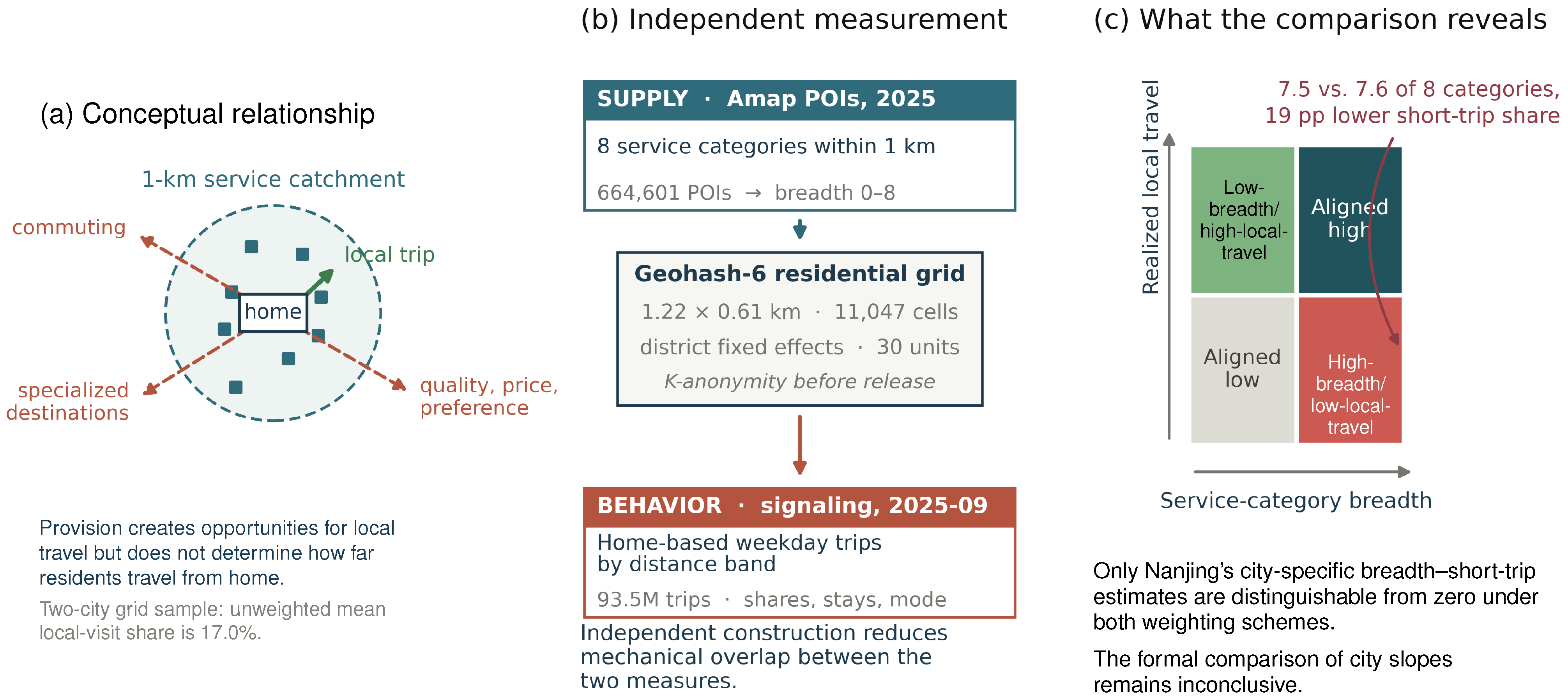
Building on studies that link accessibility with observed mobility [8,9,10,11], the harmonized three-city design combines cross-context comparison with a grid-level alignment typology and adjusted estimation. The typology preserves the spatial pattern of alignment and divergence. Adjusted and city-specific models examine whether the association persists after accounting for observed neighborhood differences and whether it varies across the three cases. Sensitivity analyses assess how strongly the diagnosis depends on alternative supply measures, catchments, spatial domains, weighting and inference procedures. Together, these analyses provide a comparative diagnostic for identifying areas that warrant closer local investigation. Figure 1 summarizes the analytical logic.

2. Materials and Methods

2.1. Comparative Urban Contexts

The feasible city set was constrained by access to comparable, privacy-protected grid-level signaling aggregates from the same operator and processing platform. Within this feasible set, Shenzhen, Nanjing, and Xuzhou were selected purposively to retain measurement comparability while capturing variation in urban scale, density and internal spatial structure. The comparison includes a dense megacity with extensive service coverage (Shenzhen), a large metropolis with pronounced core–periphery variation (Nanjing), and a lower-density prefecture-level city organized around a compact core, county seats and an extensive periphery (Xuzhou). Their mean service-breadth scores are 7.35, 5.84, and 4.86 out of eight categories, respectively (

Table 1. Study contexts and grid-level descriptive statistics. Continuous variables are reported as means, with SDs in parentheses.

	Shenzhen	Nanjing	Xuzhou
Spatial coverage
Residential analysis grids	2022	3872	5153
Travel behavior (home-based weekday trips)
Share of trips ≤2 km	0.370 (0.125)	0.205 (0.144)	0.145 (0.128)
Share of trips ≤1 km	0.240 (0.098)	0.123 (0.112)	0.067 (0.090)
Share of trips >5 km	0.321 (0.130)	0.581 (0.182)	0.574 (0.154)
Mean trip distance (km)	8.61 (2.88)	13.23 (5.15)	10.58 (3.47)
Trips per user per day	0.555 (0.134)	0.620 (0.144)	0.543 (0.145)
Neighborhood service breadth (1-km catchment)
Service breadth (0–8)	7.35 (1.51)	5.84 (2.30)	4.86 (2.65)
POI count within 1 km	846 (946)	197 (405)	102 (245)
Distance to nearest bus stop (m)	301 (268)	405 (348)	979 (1018)
Share of grids with a metro station within 800 m	0.433	0.197	0.045
Sociodemographics and urban form
Estimated residents	8307 (9630)	2242 (3682)	1417 (2606)
Mean resident age	36.5 (2.6)	41.5 (6.1)	45.8 (5.5)
Average revenue per user (ARPU; CNY/month)	48.7 (6.6)	41.7 (8.9)	33.4 (7.2)
Local-registration share	0.772 (0.081)	0.805 (0.146)	0.887 (0.098)
Jobs–housing balance score (0, 1]	0.414 (0.217)	0.444 (0.228)	0.398 (0.221)
Distance to primary center (km)	23.0 (10.8)	29.3 (20.1)	56.6 (32.1)

Note: Trip and subscriber-derived measures refer to September 2025; Amap POIs and public-transport data are from 2025. Trip measures are derived from home-based weekday trips in the mobile-phone signaling data. Supply is measured within 1 km of grid centroids.

). Because the cases were selected purposively and all lie in eastern China, they are illustrative rather than a probability sample of Chinese cities. Transfer to other regional and urban contexts requires local validation (Section 4.7).

2.2. Data Integration and Spatial Units

The design combines four source families. They comprise operator-derived mobility and sociodemographic aggregates for September 2025, 2025 Amap POIs and public transport, urban-form covariates, and an OpenStreetMap pedestrian network. We apply the same definitions, thresholds and processing steps in every city. POI coordinates are converted from GCJ-02 to WGS-84, and external attributes are linked only to privacy-protected Geohash-level aggregates released by the operator.

2.3. Mobile Phone Signaling Data and Travel Outcomes

Travel outcomes come from anonymized China Unicom signaling records processed on the operator’s Data-as-a-Service (DaaS) platform for September 2025. Stays, trips, home grids, and work grids are inferred from tower transitions and monthly temporal regularities. Only Geohash-6 aggregates (≈1.22 km × 0.61 km), constructed from Geohash-7 primitives, leave the platform. A home-based weekday trip begins in the user’s inferred home grid on a weekday. Trips are summarized by origin grid in 19 distance bands. After the filters in Section 2.6, the data contain 93.5 million trips across 11,047 residential grids (Table 1). The primary outcome is the share of trips with travel distances of 2 km or less. Secondary outcomes are the corresponding shares at 1- and 3-km thresholds, the share of trips with travel distances greater than 5 km, mean trip distance and trips per active user per day.

Although provision is measured within 1 km, the primary travel outcome uses a 2-km band to reduce sensitivity to the signaling data’s detection floor. The platform does not reliably capture movements of approximately 300 m or less, which can disproportionately affect sub-kilometer shares; the apparent degree of truncation also varies across cities (Section 4.3). The broader band reduces the relative influence of such movements while preserving a local-distance interpretation. At the same time, the two thresholds are not coterminous: trips between 1 and 2 km may extend beyond the provision catchment. Accordingly, the model relates origin-neighborhood breadth to the tendency for travel to remain local rather than attributing individual trips to the indexed POIs. Results using 1- and 3-km outcomes assess the sensitivity of the association to this scale choice (Section 3.3).

Supplementary aggregates are available only for Xuzhou and Shenzhen (7175 grids, including 7165 with complete covariates). They include a 1.1-km local-visit share (the home-grid mean of residents’ shares of away-from-home stays within 1.1 km), mode-classified distance-band counts, age- and ARPU-grouped distance bands, population-expansion-weighted outcomes, and a separately generated all-origin trip aggregation. The local-visit measure is conceptually related to the local-use outcome of Abbiasov et al. [9], but differs in coverage. Their measure includes selected consumption trips inside a pedestrian-network isochrone, whereas ours covers all detected away-from-home stays within a fixed radial distance without identifying the destination type. For mode-specific outcomes, metro trips are identified directly, whereas walking, cycling/e-bike, bus, and car trips are inferred from speed–duration–distance rules after excluding movements below 300 m and records with anomalous speeds. Although rule-based mode inference is common in signaling-data studies [51], our classifier was not validated against an external ground-truth sample. To assess sensitivity to the unresolved cycle/e-bike category, Section 3.4 presents three alternative codings. For demographic comparisons, the exports retain age (19–34, 35–59, 60+) or ARPU (low, middle, high) by home grid. Because supplementary aggregates are unavailable for Nanjing, where the trip-weighted breadth estimate is largest, these analyses extend outcome measurement only to Shenzhen and Xuzhou (Section 3.4).

2.4. POI-Based Neighborhood Service Configuration

The supply measure uses 664,601 Amap POIs (2025), harmonized through a crosswalk guided by the facility domains listed in the Chinese national life-circle standard [52]. The resulting eight analytical categories are study-specific. They are (1) education, (2) health care, (3) grocery retail, (4) dining, (5) sports and recreation, (6) culture and training, (7) parks and scenic areas, and (8) daily life and financial services. In a related study of Shanghai, Weng et al. [6] used six broad service groups. Our eight study-specific categories do not correspond one-to-one with the six conceptual functions in the original 15-min city formulation [1]. The two schemes overlap in their coverage of daily living, care, education, recreation and essential supplies. For consistent POI coding, the crosswalk distinguishes grocery retail from other everyday commercial and financial services and combines parks with scenic sites.

For grid i, $n_{ik}$ is the number of POIs in category k and $I_{ik}=1$ when $n_{ik}>0$ within 1 km of the centroid. The 1-km radius is a policy-informed operational scale, not a literal conversion of 15 min. Short-course gait speeds reported for adults and older adults are arithmetically equivalent to approximately 0.85–1.3 km over 15 min if sustained [53], while the Chinese national standard specifies an 800–1000 m walking-distance range for the 15-min level [52]. Neither reference indicates how far residents actually walk outdoors. Realized walking distance varies by trip purpose and population group [32], while route and network representation affect mapped access [3,7]. We, therefore, repeat the analysis at 800 and 1200 m and with a pedestrian-network catchment. The focal breadth score is

$$C_i={\displaystyle \sum _{k=1}^8}{I}_{ik}.$$

(1)

Thus $C_i\in \{0,\dots ,8\}$ is a binary category-coverage adaptation of a cumulative-opportunity measure and represents service-category breadth [17,18,19]. Throughout the text, provision is the umbrella concept. Breadth is the focal metric, while intensity and diversity are distinct supply dimensions. In the binary score, one facility and one hundred facilities in the same category contribute equally.

We assess this quantity limitation using a nested family of supply measures. For the common-cap score $C_i^{\left(m\right)}={\sum }_{k}min(n_{ik},m)/m$, we evaluated every integer cap from $m=1$ through $m=10$ and report $m\in \{1,2,3,5,10\}$ as representative anchors. The sequence is deliberately denser at the low end ($m=1,2,3$), where the score first departs from binary presence, and then widens ($m=5,10$) to cover moderate and larger within-category counts while retaining an upper cap; $m=1$ reproduces breadth. The five reported anchors were specified before the models were rerun. The category-balanced score $C_i^{\left(\log 95\right)}={\sum }_{k}min\{\log (1+n_{ik})/\log (1+q_{k,95}),1\}$ instead scales each category by the 95th percentile of its positive counts before equal-weight aggregation. Both study-designed transformations are informed by general composite-indicator guidance on skewness, extreme values and normalization [54]. They retain within-category quantity variation below their caps while limiting the influence of high-count categories and extreme cells. For comparison, log total POIs and POI-mix entropy enter separate models to represent intensity and diversity. Supplementary Tables S1–S11 and Figure S1 present the detailed robustness, interaction, diagnostic and predictive results referenced below.

A narrower hierarchy check uses two consistently coded fine-category tags, indicating whether a grid lies within 1 km of either a Grade III-A hospital or a scenic site with a national, provincial, or World Heritage designation. Models examine how the estimated coefficient on $C^{\left(\log 95\right)}$ changes after joint adjustment for both tags (Table S10). Because these tags cover only two domains, they provide a limited hierarchy check rather than a common measure of facility capacity, grade, or experienced quality. Breadth likewise records broad-domain coverage without distinguishing non-substitutable subservices [4]. A consistent floating-catchment measure would require harmonized capacity and competing-demand data across all eight categories, which are unavailable here. For the network sensitivity analysis, grid centroids and POIs are snapped to an OpenStreetMap pedestrian graph that excludes motorways and trunk roads, and availability is calculated from multi-source shortest paths, including the snapping legs.

2.5. Planning Context and Covariates

The covariates include estimated residential population, mean age, the grid-level mean of subscriber ARPU (average revenue per user), local-registration share, bus-stop distance and an 800-m metro-station indicator. ARPU is retained as an operator-derived billing indicator and is not treated as a validated measure of household income. We also include a symmetric jobs–housing balance index, operationalized here as $min(J/H,H/J)\in (0,1]$. This transformation draws on the classic jobs–housing balance concept [55]. Distance to the primary center (Xinjiekou, Futian Civic Center or Pengcheng Square) completes the covariate set.

2.6. Sample Construction

Within each administrative city, we retain cells with at least 100 home-based weekday trips and at least 20 users whose inferred home is in the cell during the month. These thresholds exclude cells with little detected residential activity and reduce instability from sparse counts. Table 1 presents the resulting city-specific sample and descriptive statistics.

2.7. Empirical Strategy

2.7.1. Mapping Provision–Travel Alignment

We rank breadth and short-trip share within each city, assigning average ranks to ties. We classify percentile ranks of at least 0.5 as high and ranks below 0.5 as low. Within-city ranking prevents cross-city level differences from determining the classification. The resulting four descriptive categories are aligned high, aligned low, high-breadth/low-local-travel and low-breadth/high-local-travel. We refer to the two off-diagonal categories by these descriptive labels throughout. They are screening diagnostics for local investigation; the labels do not identify the source of the divergence.

To assess dependence on the supply construct, we repeat the classification with common-cap scores, the category-balanced count score and log total POIs, as well as under tercile cut points and network-based service breadth (Table S4). We summarize pooled and city-specific agreement using Cohen’s $\kappa$ and class-specific Jaccard overlap. To test whether parks and scenic sites dominate the counted POI profiles, we compare low-breadth/high-local-travel grids with aligned-low grids on the same low-breadth side of the city cut. POI-composition measures include presence, count, composition share and majority status. Tables S9 and S11 present results from clustered park/scenic composition comparisons, alternative supply-score and cut-rule checks, park-subtype models and wider-catchment analyses. These analyses examine the POI-composition measures available in the data. Destination links, facility area, quality and visitor volume would be required to test attraction to a particular popular site.

Provision–travel divergence is measured with a continuous rank-divergence index, defined as breadth percentile rank minus short-trip percentile rank. For each city, we calculate global Moran’s I and local Moran statistics [56]. Our implementation uses row-standardized $k=8$ nearest-neighbor weights and 999 permutations. Local-cluster shares are reported both at pointwise $p<0.05$ and after within-city Benjamini–Hochberg false-discovery-rate control. We separately compute global Moran’s I for preferred-model residuals at $k=4,8,12$ to diagnose remaining spatial dependence.

2.7.2. Baseline Specification

Our baseline is a linear model of the short-trip share (expressed as a percentage) on the service-breadth score:

$$Y_{iz}=\beta {\mathrm{Breadth}}_{iz}+{\mathbf{X}}_{iz}^{\prime }\gamma +{\mu }_z+{\epsilon }_{iz},$$

(2)

where i indexes grid cells and z indexes districts (county-level units). $\mathbf{X}$ contains the covariates in Section 2.5, and ${\mu }_z$ denotes district fixed effects. The coefficient $\beta$ is estimated from within-district variation. Standard errors are clustered by district.

Because the pooled sample contains only 30 districts (Shenzhen 9, Nanjing 11, Xuzhou 10), with still fewer clusters in city-specific models, focal significance statements use null-imposed wild cluster bootstrap-tp-values with CR1 studentization and Rademacher weights [57]. Pooled and joint tests use 9999 seeded draws, while the headline single-city M5/M6 tests enumerate all $2^G$ sign patterns. Spatial dependence is examined separately by calculating spatial heteroskedasticity-and-autocorrelation-consistent (spatial-HAC) standard errors for the preferred model after within-district demeaning, using a Bartlett kernel with prespecified 5- and 10-km cutoffs.

On a fixed 11,027-cell sample, the specification ladder moves from the raw gradient to the full fixed-effects model. Trip weighting contrasts the average grid with the average represented trip, whereas separate models examine intensity and diversity as alternative supply dimensions. Breadth and log POI count are strongly correlated ($r=0.89$). Given the remaining potential for residential sorting and endogenous facility location [37,38], $\beta$ is interpreted as an adjusted association.

2.7.3. Auxiliary Nonlinear and Cross-City Prediction Check

We use gradient boosting to explore whether the fitted relationship varies systematically across breadth levels. An XGBoost regressor [58] predicts the short-trip share from service breadth, the covariates, and city indicators using 600 trees, a maximum depth of 6, a learning rate of 0.05, and row- and column-subsampling rates of 0.8. Shuffled five-fold cross-validation gives $R^2=0.68$ within the pooled sample. The primary leave-one-city-out specification omits city indicators and evaluates predictive performance in each held-out city (Section 3.2.3). Shapley additive explanations (SHAP) values [59] summarize the model-attributed contribution of service breadth in Supplementary Figure S1.

2.7.4. Heterogeneity and Robustness

We re-estimate Equation (2) by city, in place- and trip-weighted forms, and across terciles of neighborhood ARPU and mean age. Robustness checks then vary the outcome, supply definition, sample and weighting scheme. The outcome checks use the 1- and 3-km shares, mean distance and the >5 km share. Supply checks include 800- and 1200-m radii, network-based breadth, the full common-cap diagnostic path $C^{\left(m\right)}$ for $m=2,\dots ,10$, with $m=2,3,5,10$ retained as reporting anchors, the category-balanced $C^{\left(\log 95\right)}$, and standardized breadth, intensity and diversity. Sample checks impose either a 500-trip floor or a 30-km central-city restriction, while weighting checks include the effective sample size and upper-capped trip weights. For weights $w_i$, the Kish effective sample size is ${\left({\sum }_i{w}_i\right)}^2/{\sum }_i{w}_i^2$. Supply dimensions enter separate models, with the joint breadth–intensity model serving as a collinearity diagnostic.

Within the pooled Xuzhou–Shenzhen subsample, additional analyses examine the local-visit share and mode-specific short-trip shares, with robustness checks using a separate all-origin re-extraction and population-expansion weights. Demographic heterogeneity is assessed in two ways. One design estimates group-specific, trip-weighted district-fixed-effects gradients. The other uses breadth-by-group interactions with home-grid fixed effects to test whether within-grid group gaps vary with breadth. The interaction design absorbs grid-level main effects but leaves group-specific confounding unresolved. Both designs use district-clustered standard errors and are also estimated by city (Section 3.4). Inference follows the clustered, spatial-HAC and wild-bootstrap procedures above. Each table states its exact p-value convention. Tables S1 and S2 in the Supplementary Materials present the full city-specific robustness and interaction estimates.

3. Results

3.1. Where Provision and Local Travel Diverge

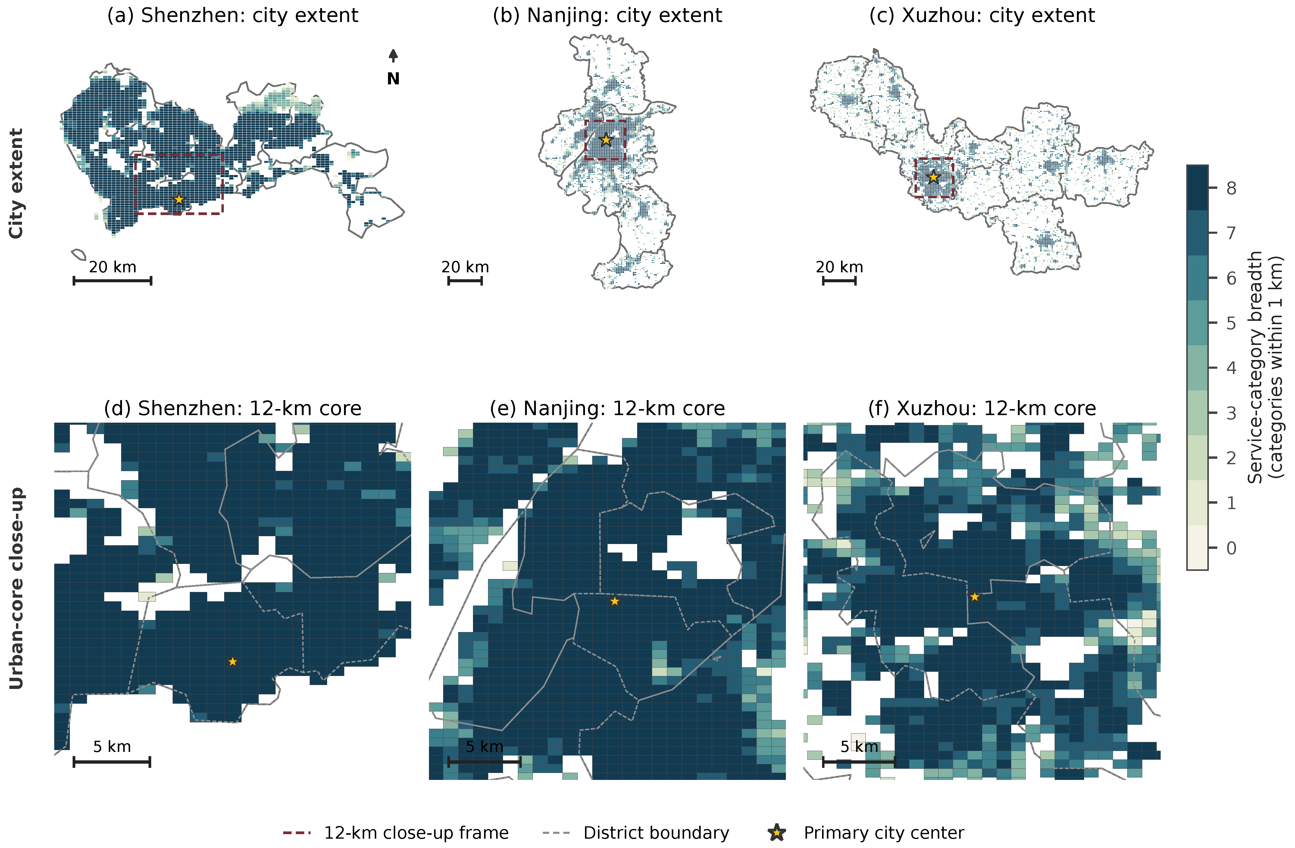
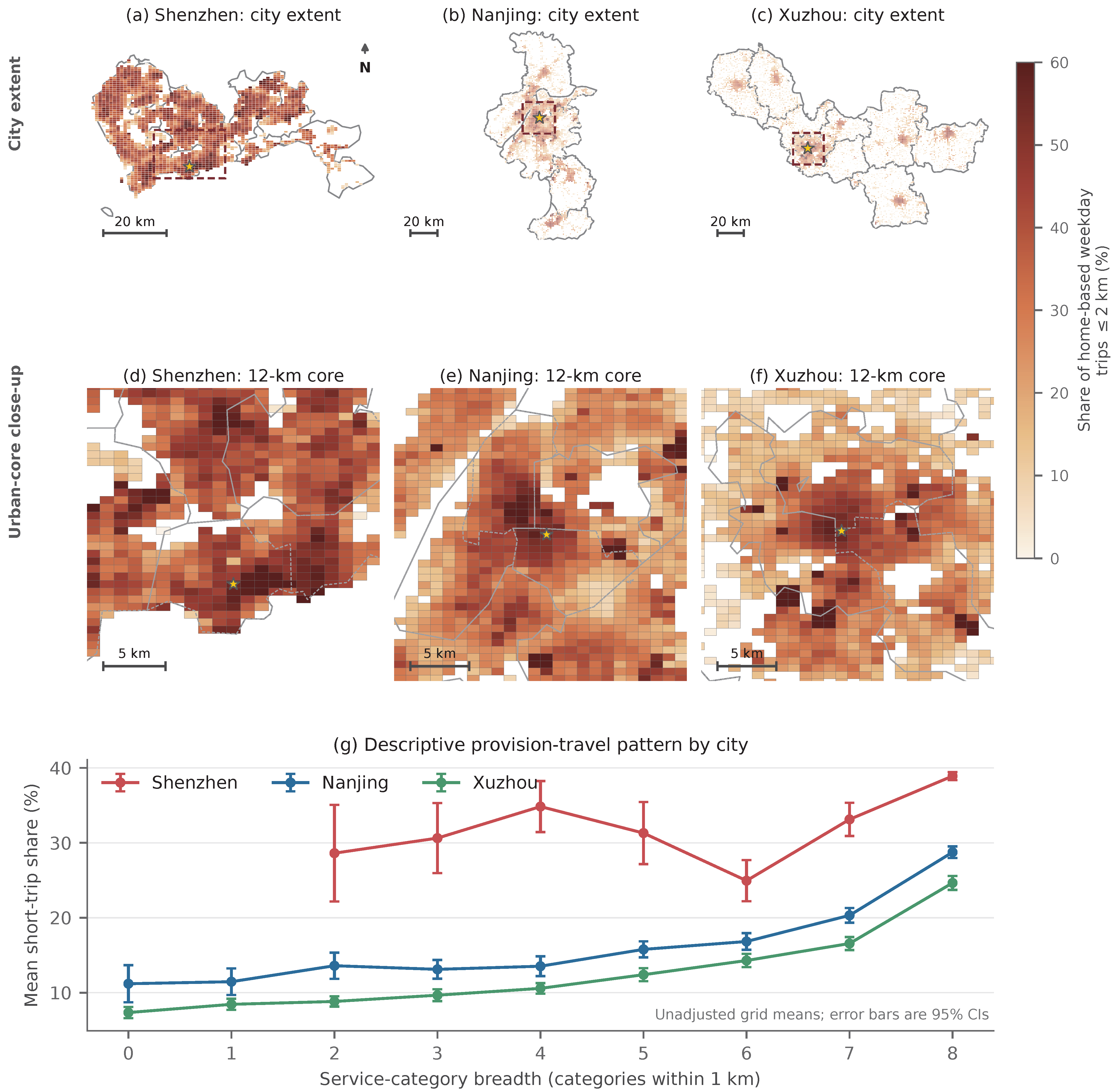
Service-category breadth follows a center–periphery gradient in all three cities, but at markedly different levels (Figure 2). Near-complete service-category coverage characterizes most of Shenzhen’s urbanized area. Nanjing combines a high-breadth core with a lower-breadth periphery, while Xuzhou concentrates high breadth in its historic core and county seats. Short-trip shares overlap with this pattern only partly (Figure 3). Binned short-trip means are generally higher at greater breadth, but the relationship is non-monotonic in some cities and differs at the upper end.

The High-Breadth/Low-Local-Travel Category

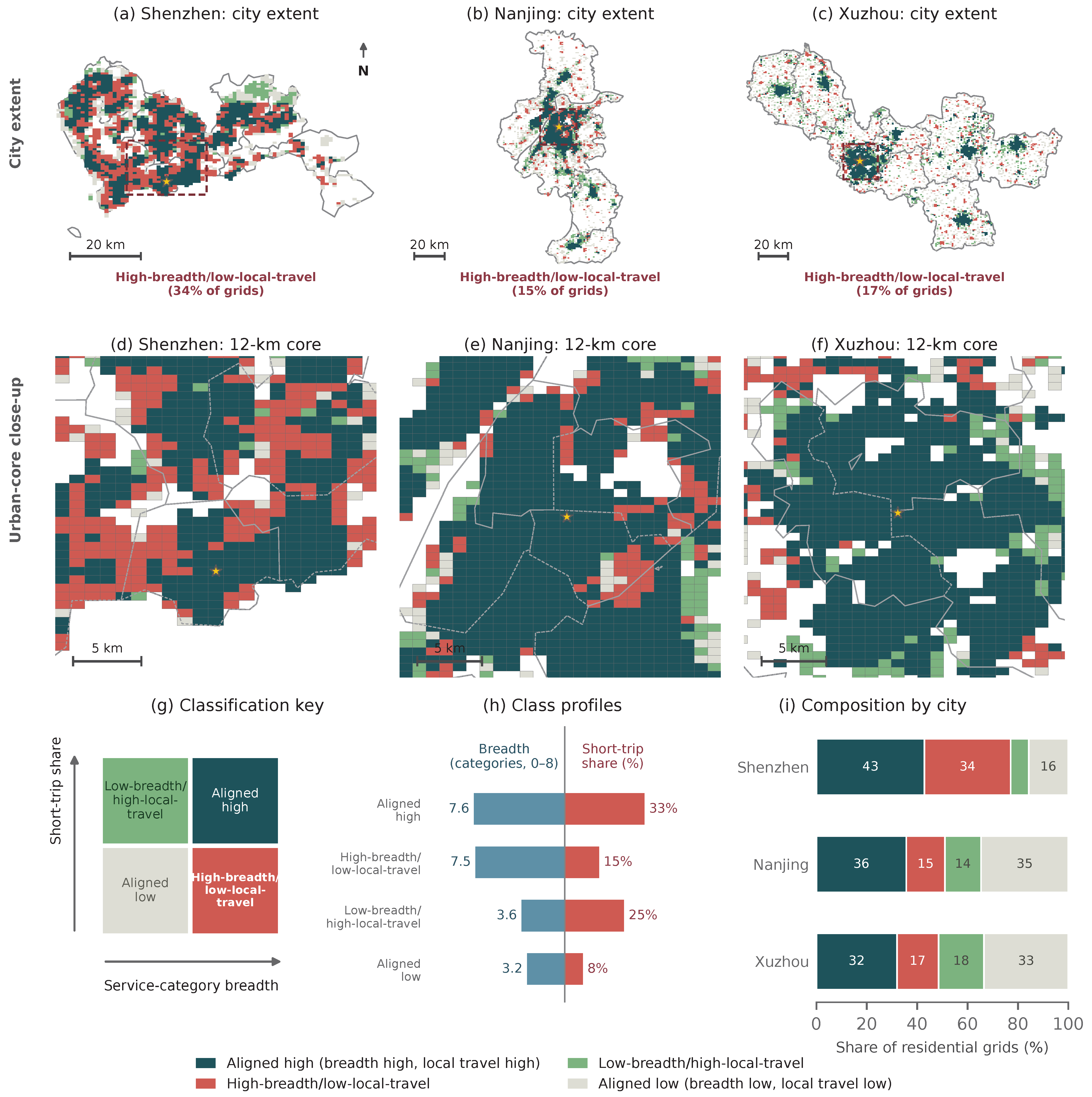
Figure 4 divides grids by their within-city breadth and short-trip percentile ranks. The classification divides the sample into aligned categories (66.0%), low-breadth/high-local-travel grids (14.8%), and high-breadth/low-local-travel grids (19.3%). Although high-breadth/low-local-travel grids average 7.49 out of eight categories, close to 7.63 in aligned-high grids, their short-trip shares differ by about 19 percentage points (14.6% versus 33.5%). Low-breadth/high-local-travel grids, by comparison, average 3.65 categories and a 25.0% short-trip share.

Among grids on the low-breadth side of the city cut, park/scenic POIs occur in 20.36% of low-breadth/high-local-travel grids and 20.03% of aligned-low grids (difference 0.33 points, 95% district-cluster bootstrap CI $-3.01$ to 3.79). They account for a majority of all counted POIs in only 0.61% and 1.60% of grids. This composition result persists across alternative supply scores and stricter cut rules (Table S9). The wider-catchment checks qualify this pattern. At 2 km, low-breadth/high-local-travel grids have higher park/scenic presence (64.26% versus 54.89%), although 35.74% still contain none. The conditional estimates are imprecise under district wild-cluster inference, and the zero-park comparisons at this wider catchment are exploratory (Table S11). At 1 km, the count profiles do not suggest simple park/scenic dominance, but attraction to an individual large or popular site remains plausible. The high local-travel shares of these grids, therefore, call for local functional assessment alongside the breadth score.

The high-breadth/low-local-travel category contains 2136 grids and accounts for 19.6% of recorded home-based weekday trips. Its incidence is highest where breadth is most saturated. It covers 34.2% of Shenzhen grids, compared with 16.5% in Xuzhou and 15.3% in Nanjing (panel (i)). Panels (a)–(f) show coherent spatial organization of the divergence. In Shenzhen, the high-breadth/low-local-travel grids form contiguous bands through the western and central districts. In Nanjing and Xuzhou they concentrate at the edge of the high-breadth core and around outlying centers. Global Moran’s I on the continuous rank-divergence index indicates spatial clustering in each city (Shenzhen 0.453, Nanjing 0.475, Xuzhou 0.390, $p=0.001$ under 999 permutations). At the unadjusted pointwise 5% threshold, local Moran statistics assign 15.68–16.52% of grids per city to high–high clusters and 12.52–14.49% to low–low clusters. Within-city Benjamini–Hochberg control reduces these ranges to 9.15–10.36% and 6.27–9.04%, respectively (Table S3). Spatial concentration remains after false-discovery-rate correction.

Membership near the 0.5 percentile-rank cut is sensitive to small rank differences and the groups also differ in composition. High-breadth/low-local-travel grids are farther from the center than aligned-high grids (39.3 km versus 31.0 km) and contain fewer residents. Section 3.2 adjusts for these observed differences.

3.2. The Adjusted Association and Its Contextual Variation

3.2.1. Specification Ladder

Adjustment sharply attenuates the provision–travel association (

Table 2. Provision–travel estimates across model specifications (outcome: share of home-based weekday trips ≤2 km; coefficients in percentage points).

	M1	M2	M3	M4	M5	M6
Service breadth (0–8)	3.098 ***	2.234 ***	0.567 ***	0.353 ***	0.301 ***	0.960 ***
	(0.275)	(0.209)	(0.137)	(0.113)	(0.111)	(0.299)
Log population			4.193 ***	4.184 ***	4.051 ***	4.651 ***
			(0.218)	(0.253)	(0.251)	(0.495)
Mean resident age			−0.709 ***	−0.661 ***	−0.698 ***	−0.906 ***
			(0.050)	(0.047)	(0.063)	(0.147)
Log ARPU			−2.836 **	−4.432 ***	−4.264 ***	−7.107 **
			(1.289)	(1.304)	(1.347)	(3.528)
Local-registration share			−1.632	0.652	−0.660	−35.803 ***
			(3.809)	(3.888)	(4.133)	(3.928)
Log distance to bus stop				−0.091	−0.005	−0.271
				(0.184)	(0.179)	(0.334)
Metro within 800 m				2.265 **	1.456 *	−0.426
				(0.894)	(0.778)	(0.564)
Jobs–housing balance score				7.509 ***	6.934 ***	8.714 ***
				(0.781)	(0.664)	(1.645)
Log distance to the primary center				−0.558	−2.890 **	−2.236
				(0.890)	(1.323)	(2.901)
City fixed effects		✓	✓	✓
District fixed effects					✓	✓
Trip-weighted						✓
N	11,027	11,027	11,027	11,027	11,027	11,027
$R^2$	0.249	0.385	0.557	0.572	0.601	0.589

Note: OLS/WLS estimates for the fixed 11,027-cell sample. District-clustered SEs are in parentheses. M5 is place-based and M6 is trip-weighted. Blanks denote excluded terms. Stars indicate significance based on cluster-robust normal p-values. Wild cluster bootstrap p-values for service breadth are in Table 3. * $p<0.1$, ** $p<0.05$, *** $p<0.01$.

). The raw gradient is 3.10 percentage points (pp) of short-trip share per additional category. It falls to 2.23 pp with city indicators, 0.57 pp with sociodemographic composition, 0.35 pp with transit and urban form, and 0.30 pp with district fixed effects. After adjustment for population composition, urban form, location and district intercepts, the fully adjusted M5 coefficient is about 90% smaller than the raw gradient. Trip weighting yields a larger estimate of 0.96 pp and changes the estimand from the average grid to the average represented trip. Across the observed 0–8 range, the two coefficients imply descriptive differences of 2.4 and 7.7 pp, equivalent to about 12% and 20% of their respective outcome means. These magnitudes summarize fitted cross-sectional contrasts; estimating responses to a facility intervention would require longitudinal evidence. Under the wild-cluster-bootstrap inference used for the focal tests, the M5 and M6 coefficients remain statistically distinguishable from zero ($p_b=0.018$ and $p_b=0.004$;

Table 3. City-specific estimates with small-cluster inference.

	Sample	$\hat{\mathit{\beta }}$	SE	p (Normal)	p (Bootstrap)	Clusters
Panel A: place-based (M5)
	Pooled	0.301	(0.111)	0.007	0.018	30
	Shenzhen	0.610	(0.482)	0.206	0.219	9
	Nanjing	0.578	(0.140)	<0.001	0.012	11
	Xuzhou	0.042	(0.126)	0.737	0.740	10
	Shenzhen–Xuzhou	0.169	(0.126)	0.178	0.197	19
Panel B: trip-weighted (M6)
	Pooled	0.960	(0.299)	0.001	0.004	30
	Shenzhen	0.020	(0.431)	0.962	0.961	9
	Nanjing	1.669	(0.351)	<0.001	0.012	11
	Xuzhou	0.250	(0.410)	0.542	0.553	10

Note: Each row estimates Equation (2) with district fixed effects, full covariates, and district-clustered SEs. p (normal) uses the cluster-robust normal approximation. p (bootstrap) uses a null-imposed wild cluster bootstrap-t [57] with full refitting and CR1 studentization. Pooled and two-city rows use 9999 seeded Rademacher draws. Single-city rows enumerate all $2^G$ sign patterns.

).

The covariate estimates show that grids with larger estimated populations and lower mean resident age have higher adjusted short-trip shares, while mean ARPU is negatively associated with the outcome. The study-specific jobs–housing balance score is positively associated with the short-trip share (+6.9 pp across its full scale), a direction compatible with the broader balance argument in Cervero [55]. Two covariates change substantially between M5 and M6. The local-registration coefficient moves from −0.66 to −35.80, while metro proximity shifts from +1.46 to −0.43. Because trip weights span three orders of magnitude, a small number of high-volume grids receive substantial aggregate weight. M6, therefore, targets the average represented trip, while M5 targets the average grid; their covariate coefficients refer to different weighted populations. Weight concentration is substantial, as shown by a Kish effective sample size of 1885, equivalent to 17.1% of the nominal cell count, and by the highest-volume 1% of cells carrying 15.2% of total weight. Capping weights at the 99th and 95th percentiles raises the effective sample size to 2150 and 2861 while leaving the corresponding coefficients close to the estimate obtained with uncapped weights (0.94 and 0.89 pp versus 0.96 pp). Weight capping retains the trip-weighted design but shifts the estimand slightly by limiting the influence of the largest cells.

3.2.2. City Point Estimates and Estimation Conditions Differ

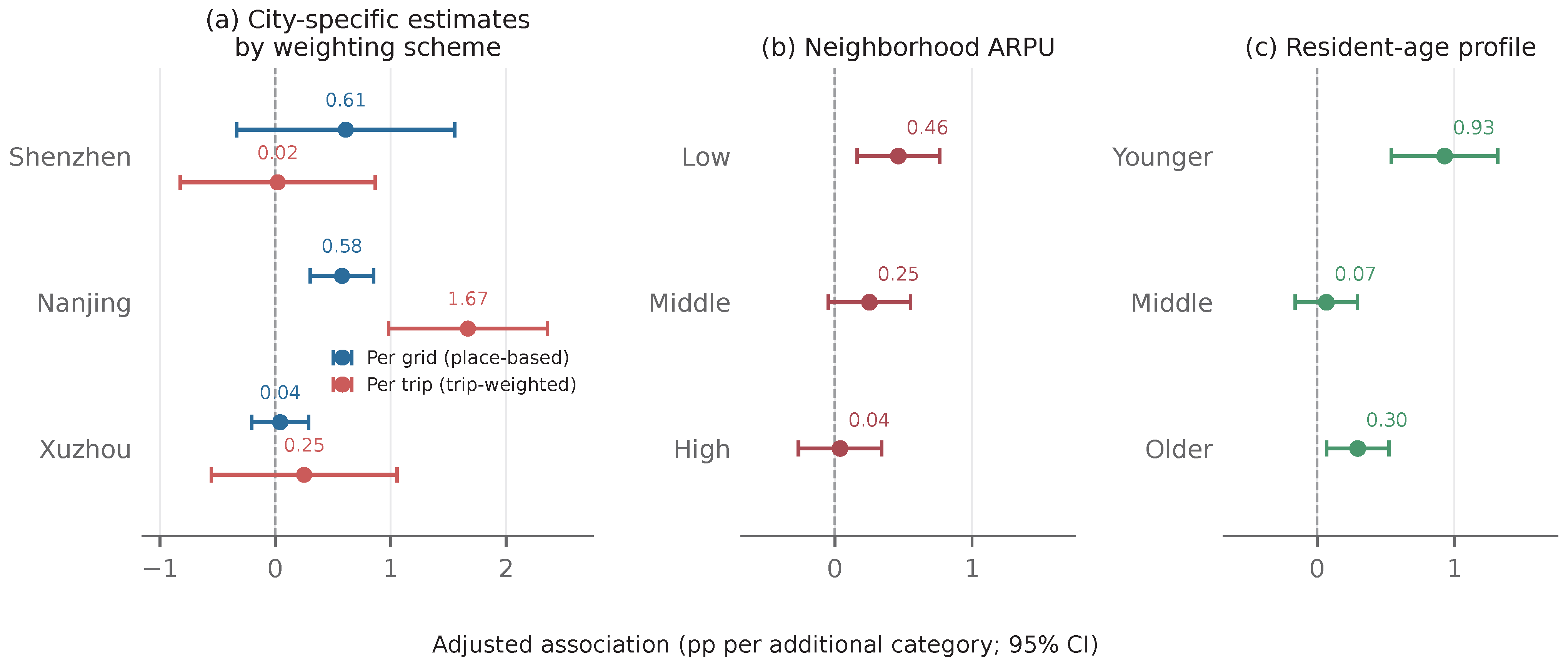
The city-specific point estimates differ (Table 3). In the place-based model, the estimates are 0.58 pp in Nanjing, 0.61 pp in Shenzhen and 0.04 pp in Xuzhou. Trip weighting changes them to 1.67, 0.02 and 0.25 pp, respectively. Although Shenzhen accounts for 60.2% of recorded trips, the pooled 0.96 pp coefficient comes from the combined weighted data and is not an average of the three city estimates. Under city-specific wild-cluster inference, the Nanjing estimate is distinguishable from zero, whereas the Shenzhen and Xuzhou estimates are not. Even so, the joint tests leave differences among the city slopes unresolved ($p_b=0.163$ for M6 and $p_b=0.849$ for M5), as shown in Table S7. Small-cluster bootstrap inference materially changes the reported p-values. Nanjing’s place-based normal-reference p-value is $3.7\times {10}^{-5}$, compared with 0.012 under the wild-cluster procedure. The same two-city sample used for the supplementary outcomes also yields an imprecise place-based service-breadth estimate (Table 3). Because that sample excludes Nanjing, its imprecision is consistent with the city decomposition.

The near-zero estimates reflect different patterns in the underlying data. In Shenzhen, 77.1% of grids already contain all eight categories, leaving limited within-district breadth variation, whereas in Xuzhou breadth varies widely but is strongly coupled with settlement structure. Section 4.3 examines these distinct estimation constraints. The positive local-visit association observed in the same Xuzhou grids also shows that the result depends on which aspect of local travel is measured (Section 3.4).

3.2.3. Auxiliary Nonlinear Pattern and Cross-City Prediction

The SHAP profile rises most sharply between seven and eight categories (Supplementary Figure S1), with a median fitted-attribution swing of about 4.5 pp. Because breadth and POI intensity correlate at $r=0.89$, the profile describes model attribution in service-rich contexts with all eight categories; the marginal contribution of the final category remains unidentified. Predictive performance does not transfer equally well across cities. Leave-one-city-out evaluation yields held-out $R^2$ values of 0.39 for Nanjing, 0.27 for Xuzhou and $-0.25$ for Shenzhen (Table S8). The negative Shenzhen value shows that the fitted model predicts the held-out city worse than a mean-outcome benchmark and underscores the need for city-specific assessment of the predictive profile.

3.2.4. Neighborhood Context

Figure 5 and

Table 4. Service-breadth associations and interaction tests by neighborhood context.

Dimension	Group	$\widehat{\mathit{\beta }}$ (Separate)	SE	Interaction vs. Reference
Neighborhood ARPU	Low tercile	0.463 ***	(0.154)	reference
(within city)	Middle tercile	0.252 *	(0.153)	−0.141 (0.166)
	High tercile	0.038	(0.155)	−0.218 (0.205)
Resident age profile	Younger tercile	0.929 ***	(0.198)	reference
(within city)	Middle tercile	0.067	(0.116)	−0.512 *** (0.177)
	Older tercile	0.296 **	(0.116)	−0.836 *** (0.213)

Note: Columns 3–4 are separate estimates of Equation (2) on each subsample ($N=3668$–3682). Column 5 presents estimates from pooled breadth × group interaction models with common covariate slopes (N = 11,027). All models include district fixed effects and full covariates. SEs are clustered by district (30 clusters). Stars use cluster-robust normal p-values. * $p<0.1$, ** $p<0.05$, *** $p<0.01$.

show how the adjusted cross-sectional association varies across neighborhood contexts within cities. Panel (a) of Figure 5 repeats the city decomposition of Table 3 for reference. Point estimates decline across within-city ARPU terciles, from 0.46 pp in the bottom tercile to 0.25 pp in the middle and 0.04 pp at the top. The pooled interactions are negative but imprecise, leaving the apparent gradient uncertain. These are ecological comparisons across neighborhood contexts. Section Demographic Differences Within Neighborhoods analysis examines ARPU-group differences within the same grids.

For the resident-age-profile terciles, the point estimate is largest in the younger-profile tercile (0.93 pp), followed by the older-profile tercile (0.30 pp), and is close to zero in the middle tercile. Relative to the younger-profile tercile, both pooled interactions are negative and statistically distinguishable from zero in the normal-reference comparison based on 30 district clusters. The two-city grouped analysis below offers a more direct comparison across age groups.

3.3. Measurement Robustness and Domain Dependence

Table 5. Service-breadth associations across alternative urban samples.

Domain	Place-Based		Trip-Weighted		Sample Information
	$\hat{\mathit{\beta }}$	${\mathit{p}}_{\mathit{b}}$	$\hat{\mathit{\beta }}$	${\mathit{p}}_{\mathit{b}}$	Grids	Trips	Clusters
Full municipal sample	0.301	0.018	0.960	0.004	100%	100%	30
Distance to the primary center
Within 20 km	0.859	0.003	1.353	0.034	31%	64%	21
Within 25 km	0.836	0.006	1.660	0.023	40%	74%	22
Within 30 km	0.598	0.053	1.409	0.017	48%	81%	24
Within 35 km	0.402	0.127	1.139	0.017	56%	90%	25
Within 50 km	0.321	0.111	0.697	0.110	67%	95%	28
Residential density
≥500 residents per km2	0.387	0.080	1.103	0.012	66%	98%	30
≥1000 residents per km2	0.571	0.062	1.128	0.044	47%	96%	30
≥1500 residents per km2	1.034	0.022	1.153	0.115	39%	94%	30
≥2000 residents per km2	1.256	0.043	1.003	0.212	34%	93%	30

Note: Each row re-estimates Equation (2) on the stated sample with district fixed effects and full covariates. $p_b$ is obtained from a null-imposed, full-refit wild cluster bootstrap with CR1 studentization and 9999 seeded draws. Density equals estimated residents divided by Geohash-6 cell area. Both sample rules are defined independently of the outcome. Distance cuts may remove whole districts, whereas density cuts retain all clusters.

and

Table 6. Robustness checks and alternative supply measures (coefficients in percentage points unless stated otherwise).

	Specification	$\hat{\mathit{\beta }}$	SE	N
Panel A: outcome, catchment, sample, and weighting checks
R1	Outcome: share of trips ≤1 km	0.197 **	(0.088)	11,027
R2	Outcome: share of trips ≤3 km	0.138	(0.165)	11,027
R3	Outcome: share of trips >5 km	0.181	(0.192)	11,027
R4	Supply radius: 800 m	0.170	(0.106)	11,027
R5	Supply radius: 1200 m	0.389 ***	(0.114)	11,027
R6	Cells with ≥500 trips	0.531 ***	(0.161)	7879
R7	Within 30 km of the primary center	0.598 **	(0.260)	5281
R8	Trip-weighted WLS	0.960 ***	(0.299)	11,027
R8a	Trip weights upper-capped at the 99th percentile	0.940 ***	(0.296)	11,027
R8b	Trip weights upper-capped at the 95th percentile	0.894 ***	(0.300)	11,027
R9	Outcome: mean trip distance (km)	0.098 **	(0.039)	11,027
Panel A′: count-sensitive scores (place-based and trip-weighted)
B1	Common-cap $C^{\left(3\right)}$ ($min(n_k,3)/3$)	0.369 **/1.158 ***	(0.130)/(0.266)	11,027
B2	Common-cap $C^{\left(5\right)}$ ($min(n_k,5)/5$)	0.422 **/1.268 ***	(0.139)/(0.251)	11,027
Panel B: separate standardized supply-dimension models
S1	Service breadth (per SD)	0.759 **	(0.281)	11,027
S2	Log POI count (per SD)	1.647 ***	(0.493)	11,027
S3	POI-mix entropy (per SD)	0.549 **	(0.239)	11,027
Panel C: joint supply model (collinearity diagnostic)
D1	Service breadth, conditional on log POI count	−0.300 *	(0.163)	11,027
D2	Log POI count, conditional on service breadth	1.169 ***	(0.352)	11,027
Panel D: spatial inference and network accessibility
C1	Spatial-HAC SE, 5 km cutoff	0.301 ***	(0.098)	11,027
C2	Spatial-HAC SE, 10 km cutoff	0.301 ***	(0.115)	11,027
N1	Network-based breadth	0.011	(0.097)	11,027
N2	Network-based breadth, trip-weighted	0.293 **	(0.114)	11,027

Note: All models include district fixed effects and full covariates. SEs are district-clustered (30 clusters) unless stated. Unless otherwise noted below, stars use normal-reference p-values based on the reported SEs in Panels A, C, and D and $t_{G-1}$ values in Panel B. Wild cluster bootstrap p-values are 0.131 (R4), 0.006 (R5), 0.053 (R7), and 0.018 (baseline). Table S1 presents the complete set. R8a–R8b upper-cap the trip weights at the stated percentiles (Kish effective sample sizes 2150 and 2861, compared with 1885 for raw weights). B1–B2 replace the binary score with count-sensitive common-cap scores. The full-refit wild-bootstrap p-values for the place-based and trip-weighted versions are 0.016/$<0.001$ and 0.011/$<0.001$, respectively, and their stars follow those values. Representative common-cap anchors, the category-balanced score, and classification stability are in Table S7. S1–S3 are separate standardized-predictor models (S1 rescales the baseline). D1–D2 are from one joint model. C1–C2 use within-district spatial-HAC SEs (Bartlett kernel). N1–N2 use 1-km OpenStreetMap pedestrian-network breadth. * $p<0.1$, ** $p<0.05$, *** $p<0.01$.

summarize sensitivity checks across the urban sample, outcome definition, supply measure, catchment, weighting and inference procedure. The adjusted coefficient remains positive in the highlighted outcome, sample and weighting checks, although its magnitude and precision vary. Catchment size changes the estimate. The coefficient is 0.17 pp at 800 m ($p_b=0.131$), 0.30 pp at 1000 m ($p_b=0.018$) and 0.39 pp at 1200 m ($p_b=0.006$). The increase across radii shows that the estimate is sensitive to the operational catchment within distances commonly used for 15-min walking access. The focal coefficient remains statistically distinguishable from zero with spatial-HAC standard errors at both the 5- and 10-km cutoffs. Residual Moran’s I ranges from 0.280 to 0.578 across cities and neighbor definitions. All permutation tests yield $p=0.001$ (Table S3), indicating that substantial spatial structure remains in the cross-section.

Although radial and pedestrian-network breadth correlate at $r=0.71$, the network-based coefficient is 0.01 pp in the place-based model and 0.29 pp with trip weighting. This contrast may reflect route structure as well as pedestrian-graph completeness. OSM road-network completeness varies substantially across regions [24]. Because local graph completeness is unverified, the consistently implemented radial measure remains focal and the network estimate serves as a sensitivity check.

Alternative travel outcomes clarify the scope of the main coefficient. Coefficients for the ≤3 km and >5 km shares are small and imprecise, whereas mean trip distance rises by 0.10 km per category. These coefficients need not move in opposite directions because the short-trip share and the mean characterize different features of the distance distribution. Human mobility often combines frequent short movements with less frequent longer ones across nested spatial scales [41,42]. The aggregate outcomes do not distinguish among trip generation, substitution, and chaining; separating these processes would require trip-purpose and activity-chain data.

Across the separate single-measure models, alternative supply definitions change the magnitude without reversing the direction of the pooled association. In separate standardized models, one-SD increases in breadth, log POI count and POI-mix entropy are associated with 0.76, 1.65 and 0.55 pp higher short-trip shares, respectively (S1–S3). The estimate is largest for intensity. Because these models are estimated separately on cross-sectional data, the coefficients compare construct-specific associations. Evaluating returns to alternative investments would require a joint longitudinal design.

Across all integer common caps, the positive place-based coefficient rises smoothly from 0.76 pp per score SD at $m=1$ to 1.43 pp at $m=10$. The category-balanced count score yields 2.40 pp. For the seven protocol-specified reported measures (the five cap anchors, the category-balanced score, and log total POIs), all BH-adjusted q-values are below 0.02. As the scores place more weight on within-category quantity, the pooled magnitude increases. Because the score family blends breadth and quantity, their separate contributions remain unidentified. Nanjing retains the largest and most precisely estimated place-based association. Formal interaction tests leave differences in the city slopes unresolved for the alternative measures (Table S7).

The hierarchy tags provide a narrower sensitivity check. The regression sample contains 388 grids near a POI tagged as a Grade III-A hospital and 165 near a rated scenic site. Joint adjustment for both tags reduces the $C^{\left(\log 95\right)}$ coefficient by only 5.7%, from 2.398 to 2.260 pp per SD. The hospital tag is positively associated with short-trip share after controlling for health-POI count, whereas the coefficient on the scenic tag is not statistically distinguishable from zero. Table S10 summarizes the multiplicity adjustment, trip-weighted models, spatial inference and record-clustering checks. Together, the two hierarchy tags provide a narrow source-taxonomy check; comparable capacity or experienced-quality measures are unavailable across all categories.

The pooled typology is relatively stable across supply constructs, with an important exception in Shenzhen. Replacing breadth with $C^{\left(3\right)}$ and $C^{\left(5\right)}$ gives four-class agreement of 91.2% and 88.7%, Cohen’s $\kappa =0.878$ and 0.844, and high-breadth/low-local-travel Jaccard overlap of 0.765 and 0.706. In Shenzhen, replacing the highly tied breadth rank with $C^{\left(5\right)}$ lowers agreement to 73.2%, $\kappa$ to 0.637 and high-breadth/low-local-travel overlap to 0.539. Figure 4 is a breadth-based screening diagnostic. Table S7 presents count-sensitive alternatives to that map.

Breadth and log POI intensity correlate at $r=0.89$. In their joint model, intensity remains positive while the breadth coefficient turns negative (D1–D2). Given this collinearity, the joint coefficients are unstable and do not separate the breadth and intensity margins.

Place-Based Association Estimates Increase in Denser, More Central Samples

Chinese administrative cities include extensive rural territory. In this sample, 52% of grids lie more than 30 km from the primary center, and Xuzhou’s county-level units extend beyond 100 km. We re-estimate the model in progressively more urban samples to assess domain sensitivity. The place-based coefficient rises from 0.30 pp in the full municipal sample to 0.60 pp within 30 km and 0.86 pp within 20 km. Across density thresholds, it increases from 0.39 pp at 500 residents per km² to 1.26 pp at 2000. The trip-weighted estimates do not increase monotonically across the same thresholds.

Table 5 reports the full gradient across the tested thresholds. Distance restrictions remove whole districts. At 30 km, the cluster count falls from 30 to 24. Density restrictions retain all 30 clusters and preserve 96% of trips at the 1000-resident threshold. Despite these different effects on sample size and cluster retention, both definitions yield the same directional domain pattern in the place-based model. The full municipal coefficient combines settings in which a neighborhood-scale service metric has different practical relevance.

3.4. Complementary Evidence: Local Travel, Travel Mode, and Demographic Differences

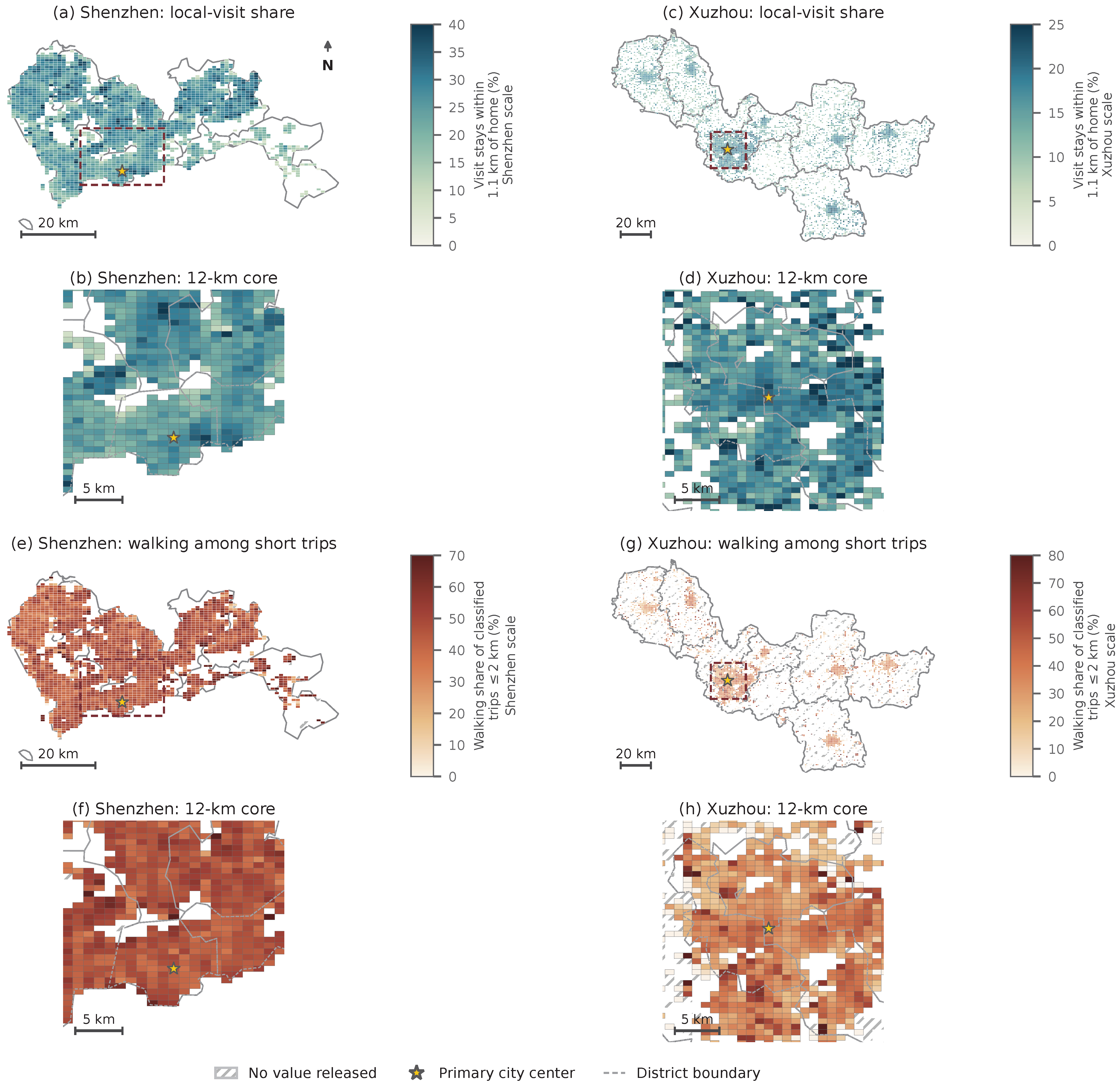
Supplementary exports from Shenzhen and Xuzhou extend the analysis by recording whether activities occur near home and how short trips are distributed across modes (

Table 7. Adjusted service-breadth associations for supplementary outcomes and pipeline checks in Shenzhen and Xuzhou.

	Outcome or Specification	$\hat{\mathit{\beta }}$	SE	N	${\mathit{R}}^2$
Panel A: local-visit share
U1	City fixed effects	0.193 ***	(0.064)	7165	0.486
U2	District fixed effects	0.158 ***	(0.061)	7165	0.515
U3	District FE, user-weighted	0.118	(0.154)	7165	0.543
Panel B: mode composition (district fixed effects)
W1	Walking share among trips ≤2 km	0.638 ***	(0.207)	5249	0.287
W1a	Walking share, with unresolved cycle/e-bike cases removed from the denominator	0.755 ***	(0.216)	5224	0.317
W1b	Walking share, with unresolved cycle/e-bike cases reassigned to walking	0.779 ***	(0.171)	5249	0.281
W1c	Walking-plus-pedal-cycling share among trips ≤2 km	0.072	(0.240)	5249	0.155
W2	Active share of ≤2 km trips	0.200	(0.154)	5249	0.094
W3	Car share of ≤2 km trips	−0.211	(0.134)	5249	0.101
W4	Active share of all trips	−0.121	(0.163)	7165	0.593
Panel C: primary-outcome and pipeline checks
B0	Original outcome, two-city subsample	0.169	(0.126)	7165	0.648
P1	Re-extracted outcome, all trips	0.188	(0.148)	7165	0.707
P2	Expansion-weighted outcome	0.220	(0.153)	7165	0.705

Note: All models include full covariates and district-clustered SEs. Panel B classifies modes from speed–duration–distance signatures (with metro trips flagged directly). Strata with <5 users are suppressed. P2 uses the operator’s population-expansion weights. Stars indicate significance based on cluster-robust normal-reference p-values. *** $p<0.01$.

). Because corresponding supplementary data are unavailable for Nanjing, these outcomes support a two-city extension rather than a three-city comparison. In the same sample, the primary breadth coefficient is 0.17 pp ($p_b=0.197$). Across the two-city grid sample, the unweighted mean local-visit share is 17.0%. The grid mean is 24.6% in Shenzhen and 14.0% in Xuzhou. The corresponding medians are 12.5% and 4.0%. Although the outcome definitions differ, this low and skewed pattern is directionally consistent with US evidence that most selected consumption trips occur beyond a 15-min walk [9]. The maps show high local-visit and walking shares across Shenzhen’s contiguous built-up area and around Xuzhou’s county seats and town centers (Figure 6).

The local-visit share records the proximity of detected away-from-home stays to home without linking those stays to the eight mapped categories. Its correlation with the short-trip share is $r=0.65$, indicating that the measures are related but distinct. Under city fixed effects, breadth is associated with a 0.19 pp higher local-visit share, compared with 0.16 pp within districts. The user-weighted estimate is smaller and imprecise at 0.12 pp. At the city level, the estimates are 0.38 pp in Shenzhen and 0.21 pp in Xuzhou, with much greater precision in Xuzhou. The positive Xuzhou local-visit estimate, alongside its near-zero short-trip coefficient, shows that the two outcomes capture different aspects of local mobility.

Mode results further narrow the interpretation. Across 5250 grids, the unweighted mean shares of classified short trips are 33.6% for walking, 83.7% under the broad active-mode definition, and 11.6% for car travel. E-bike and unresolved cycle/e-bike trips account for 25.4 percentage points, or about 30% of the reported active share (Table S5). All mode estimates are conditional on trips retained by the analysis pipeline’s rule-based classifier. Within districts, each additional category is associated with a 0.64 pp higher walking share of short trips. By contrast, the estimates for active share among short trips (+0.20 pp), car share ($-0.21$ pp) and active share across all trips ($-0.12$ pp) are imprecise. Reassigning all unresolved cycle/e-bike trips to walking or removing them from the denominator yields similar walking estimates of 0.78 and 0.76 pp (W1a–W1b), whereas the coefficient for a stricter walking-plus-pedal-cycling outcome is near zero and imprecisely estimated (0.07 pp; SE = 0.24; W1c). The W1–W3 estimates concern mode composition within short trips, whereas W4 examines the active share across all trips. The more precise result concerns walking composition within classified short trips; the broader active- and car-share estimates are imprecise.

Two pipeline checks evaluate whether relative grid-level outcome patterns remain similar under alternative aggregation schemes. An all-origin re-extraction contains 3.27 times as many trips in Shenzhen and 2.39 times as many in Xuzhou as the home-based extract. Although its outcome levels differ, correlations with the main short-trip share are 0.95 pooled, 0.95 in Xuzhou and 0.86 in Shenzhen. Its adjusted coefficient is 0.19 pp and is close to the primary estimate for the same sample. Population-expansion weighting likewise gives $r=0.95$ and a coefficient of 0.22 pp. These checks show similar relative grid-level patterns across aggregations, while operator coverage continues to constrain absolute levels and population representation.

Demographic Differences Within Neighborhoods

The grouped exports extend the analysis within neighborhoods. Each home grid contributes distance-band counts for up to nine age × ARPU cells, yielding group-by-grid aggregates rather than individual observations.

Table 8. Group-specific and within-grid demographic heterogeneity in provision–travel associations in Shenzhen and Xuzhou.

	Group or Interaction	$\hat{\mathit{\beta }}$	SE	N	${\mathit{R}}^2$
Panel A: group-specific associations
Age	19–34	1.135 **	(0.547)	6262	0.474
	35–59	0.539	(0.363)	7139	0.546
	≥60	0.909 **	(0.442)	5907	0.642
ARPU group	Low	1.042 **	(0.423)	7147	0.572
(ARPU band)	Middle	0.881 **	(0.433)	6866	0.499
	High	0.695	(0.504)	5339	0.427
Panel B: within-grid interactions
Age (ref. 19–34)	× 35–59	0.476 ***	(0.178)	19,329
	×≥60	1.532 ***	(0.256)	19,329
ARPU group (ref. low)	× middle	0.065	(0.070)	19,370
	× high	−0.109	(0.106)	19,370
Panel C: within-grid interactions by city
Shenzhen, age	× 35–59	0.632 **	(0.247)	5721
(ref. 19–34)	×≥60	1.901 ***	(0.627)	5721
Xuzhou, age	× 35–59	−0.351 ***	(0.076)	13,608
(ref. 19–34)	×≥60	0.595 ***	(0.179)	13,608
Shenzhen, ARPU group	× middle	−0.124	(0.102)	6052
(ref. low)	× high	−0.274	(0.182)	6052
Xuzhou, ARPU group	× middle	0.028	(0.032)	13,318
(ref. low)	× high	−0.350 ***	(0.102)	13,318

Note: The dependent variable is each group’s percentage of weekday home-origin trips in the 0–2 km band, calculated by grid. Panel A estimates Equation (2) by group with full covariates, district fixed effects, and trip weights. Panels B–C estimate breadth × group interactions with home-grid fixed effects using trip-weighted within-grid demeaning. Grid-level terms are absorbed. Cells with <5 users or <10 trips and users with missing attributes are excluded (missing attributes account for 21% of Shenzhen and 31% of Xuzhou trips). N counts grid-by-group cells. SEs are clustered by district (19 pooled, 9–10 by city). Stars use cluster-robust normal p-values. ** $p<0.05$, *** $p<0.01$.

presents estimates from both between-grid group-specific models and within-grid interaction models. Age shows the clearest differential pattern. The trip-weighted short-trip share is 52.0% for residents aged 60 or older, 50.0% for ages 19–34 and 48.8% for ages 35–59. In the model with home-grid fixed effects, the breadth gradient for residents aged 60 or older is 1.53 pp per category steeper than that for residents aged 19–34. This differential is positive in both cities (1.90 pp in Shenzhen and 0.60 pp in Xuzhou), whereas the contrast for ages 35–59 changes sign. Because Panel A compares neighborhoods while Panel B compares groups living in the same neighborhood, the age interpretation rests on the within-grid estimates. Grid fixed effects absorb shared spatial context, while group-specific confounding may still affect the contrasts.

ARPU-group results are less consistent. Between-grid gradients decline across ARPU bands, but the confidence intervals for both pooled within-grid interaction estimates include zero. The high-versus-low differential is negative in each city but more uncertain in Shenzhen. The mixed pattern leaves a common ARPU gradient unresolved. Assessing distributional responses to a facility upgrade would require longitudinal group-specific data.

4. Discussion

The grid comparison adds a behavioral diagnostic to conventional provision mapping. The spatial concentration of high-breadth/low-local-travel neighborhoods shows that near-complete category coverage can coexist with a local-travel percentile rank below 0.5 and indicates where follow-up is warranted. Once neighborhood composition and geography are considered, the remaining association is modest and varies with the supply metric and analytical context. These patterns make local calibration central to interpretation.

4.1. From Proximity-Oriented Provision to Realized Local Travel

The marked attenuation after adjustment indicates that the raw gradient is highly sensitive to population composition, urban form and location. A supply map remains valuable for measuring potential access; behavioral performance requires a separate outcome. Possible differences in facility quantity, capacity, quality and location offer competing explanations for the observed divergence and motivate field investigation.

The alternative distance outcome helps delimit what local travel captures. In the pooled three-city model, breadth is associated with a 0.10-km increase in mean trip distance per category, even as the short-trip share rises. The two results can coexist when mobility is organized at multiple spatial scales [41,42]. They describe the grid-level distribution of trips rather than changes in individual activity ranges.

4.2. Comparison with Prior Evidence from Nanjing

The central-city null reported by Qi et al. [10] comes from a substantially different design. Their study covers 549 small TAZs across 37.9 km² of central Nanjing and uses a two-day subset from one week of signaling records. Supply is the total count of seven essential-service POI types within 2 km, and the outcomes are non-commuting travel distance and cumulative frequency. Our analysis, by comparison, uses one month of weekday data for the full municipality, measures the 1-km presence of eight service categories, and models the share of home-based trips of 2 km or less with covariates and district fixed effects. The contrast may, therefore, reflect differences in spatial scope, observation period, supply definition, catchment, outcome or adjustment. Our sensitivity checks cover only part of this design space, leaving the source of the difference open.

4.3. Interpreting the Shenzhen and Xuzhou Estimates

Neither Shenzhen nor Xuzhou yields a city coefficient distinguishable from zero, but the underlying data conditions differ. In Xuzhou, the place-based short-trip coefficient is 0.04 across the same 5144 grids, compared with 0.21 for the local-visit outcome. The unadjusted short-trip share rises from 7.4% at zero categories to 24.7% at eight. Xuzhou’s near-zero adjusted short-trip result is specific to the selected outcome and adjustment set. Table S6 summarizes fuller diagnostics for the city-level null results, including variation available for estimation, the 1-to-2-km trip-share ratio and the alternative local-visit outcome. Adding population and distance to the center reduces Xuzhou’s coefficient from 0.76 to 0.04, compared with corresponding estimates of 0.58 in Nanjing and 0.61 in Shenzhen. Xuzhou also has the largest share of breadth variation explained by covariates and district effects (48%, versus 44% in Nanjing and 31% in Shenzhen), and its mean grid population rises from 413 residents at zero categories to 3970 at eight. This close coupling between breadth and settlement density reduces the residual variation available for estimating the adjusted association.

Shenzhen presents a different limitation. Although the controls explain a smaller share of breadth variation, widespread ceiling saturation means that its coefficient is estimated mainly from the minority of grids missing at least one category. Xuzhou’s coefficient is strongly attenuated after adjustment for settlement structure, whereas Shenzhen’s estimate is limited by breadth saturation. For Xuzhou, the trip-weighted estimate is further qualified by apparent truncation and leverage. Its ratio of ≤1 km to ≤2 km trips is 0.46, compared with 0.60 in Nanjing and 0.65 in Shenzhen, a pattern consistent with greater apparent truncation of sub-kilometer movement. The urban-district/county split yields coefficients of $+0.65$ and $-0.71$, but each subsample contains only five district clusters. Once the largest 5% of county grids by trip volume are removed, the county estimate moves to $+0.04$. This shift shows that the negative county coefficient is highly leverage-sensitive and too unstable for substantive interpretation (

Table 9. Sample-split and leverage diagnostics for the trip-weighted Xuzhou estimate.

Sample	$\hat{\mathit{\beta }}$	${\mathit{p}}_{\mathbf{normal}}$	Grids	Districts
Xuzhou, all districts	0.250	0.542	5144	10
Five urban districts	+0.649	0.110	1709	5
Five county-level units	−0.711	0.010	3435	5
County-level units excluding the top 5% of grids by trip volume	+0.035	0.831	3263	5

Note: Each row estimates Equation (2) with district fixed effects, full covariates, trip weights and district-clustered SEs. The split samples contain only five district clusters. The normal-reference p-values are descriptive post hoc diagnostics and are not used for confirmatory inference. Excluding the highest-volume county grids changes the county estimate from $-0.711$ to $+0.035$, illustrating its sensitivity to leverage from high-volume grids (Section 4.3).

).

The diagnostics point to different constraints on the city estimates. Although the formal interaction test remains inconclusive, Shenzhen’s saturation and Xuzhou’s settlement coupling still matter when interpreting the point estimates. The prediction exercise also shows limited cross-city transfer: a model trained on Nanjing and Xuzhou predicts the held-out Shenzhen sample less accurately than the benchmark based on Shenzhen’s observed mean outcome. This weak transfer to Shenzhen reinforces the need to validate externally estimated relationships in the target city.

4.4. Breadth and Intensity as Complementary Planning Diagnostics

Breadth and intensity describe different dimensions of the mapped POI inventory but are tightly coupled in these data. The larger associations under count-sensitive scores, together with reclassification in saturated Shenzhen, show that the diagnosis depends on how supply is represented. The measures serve different diagnostic tasks. Category-level presence indicators identify which service categories are absent from the mapped POI inventory, while the breadth score summarizes how many categories are represented. Capped and log-count scores distinguish differences in mapped within-category POI counts once most categories are present. The hierarchy-tag audit changes the coefficient on the category-balanced log-count score by only 5.7%, but its coverage is limited to Grade III-A hospitals and rated scenic sites. This narrow coverage makes it unsuitable as a general quality scale. Breadth and category-balanced counts can instead be reported alongside locally collected information on capacity and quality.

When breadth and log POI intensity enter jointly, intensity retains a positive coefficient while breadth reverses sign. Their correlation ($r=0.89$), conditional variance-inflation factors of 9.9–136.7 and a condition number of 34.7 indicate that this coefficient allocation is unstable. The joint model cannot distinguish the return to completing an eighth category from the return to adding depth within an existing one. Staggered additions and upgrades, evaluated with an appropriate comparison design, could provide longitudinal evidence for comparing those investment margins.

4.5. Where the Evidence Applies

City-specific trip-weighted point estimates vary substantially, but the joint interaction test does not resolve whether the slopes differ. For the place-based specification, coefficients rise as the sample is narrowed toward the urban core. The corresponding trip-weighted patterns are not monotonic, so the domain results support local calibration rather than a common density gradient across the three cities. Mode-specific results describe composition within classified trips. Their interpretation depends partly on the heuristic classifier because e-bike and unresolved cycle/e-bike journeys make up a substantial portion of the constructed active-mode measure. Interpreting these shares in terms of carbon emissions, health or congestion would also depend on direct measurements of those outcomes. The ARPU-group patterns can help identify neighborhoods for closer equity audits. Because the underlying observations are group-by-grid aggregates, the analysis cannot show how the association is distributed among individuals or changes over time.

4.6. Provision–Travel Diagnostics for Planning Practice

Planning agencies can examine these supply measures alongside local-visit measures, short-trip shares, and mode indicators. The high-breadth/low-local-travel category provides a screen for locations where capacity, affordability, opening hours, pedestrian access, and preferences merit field investigation, while the low-breadth/high-local-travel category points to omitted local conditions requiring assessment. At the focal 1-km scale, the POI profiles of the latter category show no simple park/scenic count dominance, although the wider-catchment comparison is less uniform. Because cells near either cut point can change class and the groups differ in density, population and location, the rank-based categories should guide local investigation, not resource allocation. The catchment, network, spatial-inference and small-cluster checks show how the findings depend on specific analytical choices. With repeated observations around planning changes, the same privacy-preserving framework could support longitudinal evaluation.

4.7. Limitations and Future Research

The findings are subject to five limitations.

• Cross-sectional identification. District fixed effects and observed covariates leave residential sorting [37,38] and endogenous service location unresolved. The regression estimates describe adjusted spatial associations. The alignment classes locate areas of divergence, while the effects of adding or upgrading a facility remain unidentified.
• Provision and destination measurement. The focal measure captures category breadth, while count-sensitive alternatives add within-category POI-count information and two source tags provide a narrow hierarchy check. These extensions do not establish completeness within each broad service category because a category can contain non-substitutable subservices. Comparable measures of capacity, floor area, quality, affordability, usability and popularity remain unavailable across all categories, and trips cannot be linked to POI destinations. This means that the park/scenic audits address count dominance and catchment sensitivity only. Attraction to a single large or popular destination remains possible. Breadth saturation is particularly acute in Shenzhen.
• Scale and domain dependence. At an 800-m catchment, the coefficient falls to 0.17 pp and is imprecisely estimated. It becomes larger in denser and more central samples. The focal association is most directly interpreted for service breadth measured at approximately 1 km in urban neighborhood contexts. Other settlement types require locally validated baselines.
• Spatial support, mobility measurement, and inference. The signaling pipeline may under-record movements shorter than its approximate 300-m detection threshold, with stronger signs of apparent truncation in Xuzhou. Mode is inferred heuristically in two cities and has not been validated against external ground truth. The fixed anisotropic Geohash-6 origin grid (≈1.22 km × 0.61 km) may make estimates sensitive to the modifiable areal unit problem (MAUP). The partial mismatch between the grid-based origin support and circular service catchments creates uncertainty associated with the uncertain geographic context problem (UGCoP) [25]. Because the data license prevents reprocessing individual records on an alternative grid, we could not conduct a formal regridding test. The 800/1000/1200-m and pedestrian-network checks vary the service catchment while holding the Geohash-6 origin support fixed, so they do not test sensitivity to alternative grid geometries. Inference is based on 30 districts overall and 9–11 per city, which motivates the small-cluster bootstrap checks used for the focal results.
• Temporal and geographic coverage. The data cover one month in one season. Walking accessibility can vary diurnally and seasonally [7], so the observed month may not represent other periods. Supplementary visit and mode outcomes are available for Shenzhen and Xuzhou but not Nanjing. The three purposively selected eastern Chinese cities provide analytically contrasting cases, although they are not representative of China as a whole. Generalization to other regions, seasons and urban contexts requires harmonized evidence from a broader and more representative range of settings and periods.

Future work can match each measurement gap to a more informative design. Repeated signaling panels around staggered life-circle upgrades, coupled with appropriate comparison groups, would allow travel changes to be examined after category completion, facility expansion or quality improvement. The typology could then structure stratified sampling for evaluation. Where destination links are available, combining them with facility audits, opening hours, prices, pedestrian networks and resident surveys could help distinguish limited capacity from destination competition and resident preferences. Group-specific longitudinal analyses would trace how observed changes vary across resident groups. A GPS or app-based validation sample would test the mode classification, and panels spanning seasons and regions would assess temporal and geographic generalizability. Questions about emissions, physical activity, exposure and welfare call for direct measures of those outcomes.

5. Conclusions

The analysis covers 11,047 residential grids and 93.5 million home-based weekday trips, with realized local travel defined by the proportion of those trips at or below 2 km. This outcome describes distance-band behavior rather than direct evidence of service use. Combining it with independently measured service breadth identifies 2136 high-breadth/low-local-travel grids, representing 19.3% of grids and 19.6% of trips. A 0.14-category difference in mean breadth accompanies an 18.9-percentage-point difference in short-trip share between the high-breadth/low-local-travel and aligned-high groups. The continuous rank-divergence measure is spatially clustered in all three cities, locating concentrations that warrant local investigation.

Adjustment sharply attenuates the pooled three-city relationship. The fully adjusted place-based slope is 0.30 percentage points per category, roughly one tenth of the unadjusted estimate. Count-sensitive alternatives produce different magnitudes, but their high collinearity with breadth prevents separate attribution to breadth or intensity. Changing radial or network catchments also alters the magnitude and precision of the estimates, underscoring their scale dependence. City-specific point estimates differ, and the association depends on the outcome definition. For the focal breadth–short-trip specification, Nanjing provides the only city-specific slope distinguishable from zero, while the joint city comparison is inconclusive. Place-based estimates are also sensitive to the included urban domain. The supplementary outcomes show that the short-trip share captures one dimension of mobility alongside destination proximity, mode composition, and the wider trip-distance distribution.

As a comparative screening diagnostic, the framework uses category-level presence indicators to identify which service categories are absent from the mapped POI inventory, breadth to summarize how many are represented, and count-based measures to describe mapped within-category POI quantity. Read against city-specific baselines and local evidence on capacity, quality, and travel, these measures can prioritize field investigation in high-breadth/low-local-travel areas and assessment of omitted local conditions in low-breadth/high-local-travel areas. The framework alone cannot determine whether any mapped facility should be added, expanded, upgraded, or otherwise modified. Repeated observations around planning changes, combined with an appropriate comparison design, would extend the framework from spatial diagnosis to causal evaluation.

References

1. Moreno, C.; Allam, Z.; Chabaud, D.; Gall, C.; Pratlong, F. Introducing the “15-minute city”: Sustainability, resilience and place identity in future post-pandemic cities. Smart Cities 2021, 4, 93–111. [Google Scholar] [CrossRef] [Scilit]
2. Logan, T.M.; Hobbs, M.H.; Conrow, L.C.; Reid, N.L.; Young, R.A.; Anderson, M.J. The x-minute city: Measuring the 10, 15, 20-minute city and an evaluation of its use for sustainable urban design. Cities 2022, 131, 103924. [Google Scholar] [CrossRef] [Scilit]
3. Ferrer-Ortiz, C.; Marquet, O.; Mojica, L.; Vich, G. Barcelona under the 15-minute city lens: Mapping the accessibility and proximity potential based on pedestrian travel times. Smart Cities 2022, 5, 146–161. [Google Scholar] [CrossRef] [Scilit]
4. Papadopoulos, E.; Sdoukopoulos, A.; Politis, I. Measuring compliance with the 15-minute city concept: State-of-the-art, major components and further requirements. Sustain. Cities Soc. 2023, 99, 104875. [Google Scholar] [CrossRef] [Scilit]
5. Khavarian-Garmsir, A.R.; Sharifi, A.; Sadeghi, A. The 15-minute city: Urban planning and design efforts toward creating sustainable neighborhoods. Cities 2023, 132, 104101. [Google Scholar] [CrossRef] [Scilit]
6. Weng, M.; Ding, N.; Li, J.; Jin, X.; Xiao, H.; He, Z.; Su, S. The 15-minute walkable neighborhoods: Measurement, social inequalities and implications for building healthy communities in urban China. J. Transp. Health 2019, 13, 259–273. [Google Scholar] [CrossRef] [Scilit]
7. Willberg, E.; Fink, C.; Toivonen, T. The 15-minute city for all?—Measuring individual and temporal variations in walking accessibility. J. Transp. Geogr. 2023, 106, 103521. [Google Scholar] [CrossRef] [Scilit]
8. Graells-Garrido, E.; Serra-Burriel, F.; Rowe, F.; Cucchietti, F.M.; Reyes, P. A city of cities: Measuring how 15-minutes urban accessibility shapes human mobility in Barcelona. PLoS ONE 2021, 16, e0250080. [Google Scholar] [CrossRef] [Scilit]
9. Abbiasov, T.; Heine, C.; Sabouri, S.; Salazar-Miranda, A.; Santi, P.; Glaeser, E.; Ratti, C. The 15-minute city quantified using human mobility data. Nat. Hum. Behav. 2024, 8, 445–455. [Google Scholar] [CrossRef] [Scilit]
10. Qi, C.; De Vos, J.; Guo, X.; Zhang, Y.; Guo, Y. Do nearby activities result in short trips? Examining the relationship between spatial accessibility and travel behaviour in 15-minute neighbourhoods. J. Transp. Geogr. 2026, 134, 104696. [Google Scholar] [CrossRef] [Scilit]
11. Zhang, Y.; Liu, J.; Bonino, M. What Facilities and Layout Create a 15-Minute Living Circle for Green Travel. ISPRS Int. J. Geo-Inf. 2026, 15, 276. [Google Scholar] [CrossRef] [Scilit]
12. Pozoukidou, G.; Chatziyiannaki, Z. 15-minute city: Decomposing the new urban planning eutopia. Sustainability 2021, 13, 928. [Google Scholar] [CrossRef] [Scilit]
13. Hansen, W.G. How accessibility shapes land use. J. Am. Inst. Plan. 1959, 25, 73–76. [Google Scholar] [CrossRef] [Scilit]
14. Ingram, D.R. The concept of accessibility: A search for an operational form. Reg. Stud. 1971, 5, 101–107. [Google Scholar] [CrossRef] [Scilit]
15. Wachs, M.; Kumagai, T.G. Physical accessibility as a social indicator. Socio-Econ. Plan. Sci. 1973, 7, 437–456. [Google Scholar] [CrossRef] [Scilit]
16. Morris, J.M.; Dumble, P.L.; Wigan, M.R. Accessibility indicators for transport planning. Transp. Res. Part A Gen. 1979, 13, 91–109. [Google Scholar] [CrossRef] [Scilit]
17. Geurs, K.T.; van Wee, B. Accessibility evaluation of land-use and transport strategies: Review and research directions. J. Transp. Geogr. 2004, 12, 127–140. [Google Scholar] [CrossRef] [Scilit]
18. Handy, S.L.; Niemeier, D.A. Measuring accessibility: An exploration of issues and alternatives. Environ. Plan. A 1997, 29, 1175–1194. [Google Scholar] [CrossRef] [Scilit]
19. Levinson, D.; Wu, H. Towards a general theory of access. J. Transp. Land Use 2020, 13, 129–158. [Google Scholar] [CrossRef] [Scilit]
20. Luo, W.; Wang, F. Measures of spatial accessibility to health care in a GIS environment: Synthesis and a case study in the Chicago region. Environ. Plan. B Plan. Des. 2003, 30, 865–884. [Google Scholar] [CrossRef] [Scilit]
21. Nicoletti, L.; Sirenko, M.; Verma, T. Disadvantaged communities have lower access to urban infrastructure. Environ. Plan. B Urban Anal. City Sci. 2023, 50, 831–849. [Google Scholar] [CrossRef] [Scilit]
22. Páez, A.; Scott, D.M.; Morency, C. Measuring accessibility: Positive and normative implementations of various accessibility indicators. J. Transp. Geogr. 2012, 25, 141–153. [Google Scholar] [CrossRef] [Scilit]
23. Xu, Y.; Olmos, L.E.; Abbar, S.; González, M.C. Deconstructing laws of accessibility and facility distribution in cities. Sci. Adv. 2020, 6, eabb4112. [Google Scholar] [CrossRef] [Scilit]
24. Barrington-Leigh, C.; Millard-Ball, A. The world’s user-generated road map is more than 80% complete. PLoS ONE 2017, 12, e0180698. [Google Scholar] [CrossRef] [Scilit]
25. Kwan, M.P. The uncertain geographic context problem. Ann. Assoc. Am. Geogr. 2012, 102, 958–968. [Google Scholar] [CrossRef] [Scilit]
26. Cervero, R.; Kockelman, K. Travel demand and the 3Ds: Density, diversity, and design. Transp. Res. Part D Transp. Environ. 1997, 2, 199–219. [Google Scholar] [CrossRef] [Scilit]
27. Ewing, R.; Cervero, R. Travel and the built environment: A meta-analysis. J. Am. Plan. Assoc. 2010, 76, 265–294. [Google Scholar] [CrossRef] [Scilit]
28. Stevens, M.R. Does compact development make people drive less? J. Am. Plan. Assoc. 2017, 83, 7–18. [Google Scholar] [CrossRef] [Scilit]
29. Næss, P. Urban form and travel behavior: Experience from a Nordic context. J. Transp. Land Use 2012, 5, 21–45. [Google Scholar] [CrossRef] [Scilit]
30. Marquet, O.; Miralles-Guasch, C. The walkable city and the importance of the proximity environments for Barcelona’s everyday mobility. Cities 2015, 42, 258–266. [Google Scholar] [CrossRef] [Scilit]
31. Millward, H.; Spinney, J.; Scott, D. Active-transport walking behavior: Destinations, durations, distances. J. Transp. Geogr. 2013, 28, 101–110. [Google Scholar] [CrossRef] [Scilit]
32. Yang, Y.; Diez-Roux, A.V. Walking distance by trip purpose and population subgroups. Am. J. Prev. Med. 2012, 43, 11–19. [Google Scholar] [CrossRef] [Scilit]
33. Boarnet, M.; Crane, R. The influence of land use on travel behavior: Specification and estimation strategies. Transp. Res. Part A Policy Pract. 2001, 35, 823–845. [Google Scholar] [CrossRef] [Scilit]
34. Ding, C.; Wang, D.; Liu, C.; Zhang, Y.; Yang, J. Exploring the influence of built environment on travel mode choice considering the mediating effects of car ownership and travel distance. Transp. Res. Part A Policy Pract. 2017, 100, 65–80. [Google Scholar] [CrossRef] [Scilit]
35. Ding, C.; Cao, X.; Næss, P. Applying gradient boosting decision trees to examine non-linear effects of the built environment on driving distance in Oslo. Transp. Res. Part A Policy Pract. 2018, 110, 107–117. [Google Scholar] [CrossRef] [Scilit]
36. Elldér, E.; Haugen, K.; Vilhelmson, B. When local access matters: A detailed analysis of place, neighbourhood amenities and travel choice. Urban Stud. 2022, 59, 120–139. [Google Scholar] [CrossRef] [Scilit]
37. Mokhtarian, P.L.; Cao, X. Examining the impacts of residential self-selection on travel behavior: A focus on methodologies. Transp. Res. Part B Methodol. 2008, 42, 204–228. [Google Scholar] [CrossRef] [Scilit]
38. Cao, X.; Mokhtarian, P.L.; Handy, S.L. Examining the impacts of residential self-selection on travel behaviour: A focus on empirical findings. Transp. Rev. 2009, 29, 359–395. [Google Scholar] [CrossRef] [Scilit]
39. Lucas, K. Transport and social exclusion: Where are we now? Transp. Policy 2012, 20, 105–113. [Google Scholar] [CrossRef] [Scilit]
40. Pereira, R.H.M.; Schwanen, T.; Banister, D. Distributive justice and equity in transportation. Transp. Rev. 2017, 37, 170–191. [Google Scholar] [CrossRef] [Scilit]
41. González, M.C.; Hidalgo, C.A.; Barabási, A.L. Understanding individual human mobility patterns. Nature 2008, 453, 779–782. [Google Scholar] [CrossRef] [Scilit]
42. Alessandretti, L.; Aslak, U.; Lehmann, S. The scales of human mobility. Nature 2020, 587, 402–407. [Google Scholar] [CrossRef] [Scilit]
43. Schläpfer, M.; Dong, L.; O’Keeffe, K.; Santi, P.; Szell, M.; Salat, H.; Anklesaria, S.; Vazifeh, M.; Ratti, C.; West, G.B. The universal visitation law of human mobility. Nature 2021, 593, 522–527. [Google Scholar] [CrossRef] [Scilit]
44. Barbosa, H.; Barthelemy, M.; Ghoshal, G.; James, C.R.; Lenormand, M.; Louail, T.; Menezes, R.; Ramasco, J.J.; Simini, F.; Tomasini, M. Human mobility: Models and applications. Phys. Rep. 2018, 734, 1–74. [Google Scholar] [CrossRef] [Scilit]
45. Calabrese, F.; Diao, M.; Di Lorenzo, G.; Ferreira, J.; Ratti, C. Understanding individual mobility patterns from urban sensing data: A mobile phone trace example. Transp. Res. Part C Emerg. Technol. 2013, 26, 301–313. [Google Scholar] [CrossRef] [Scilit]
46. Deville, P.; Linard, C.; Martin, S.; Gilbert, M.; Stevens, F.R.; Gaughan, A.E.; Blondel, V.D.; Tatem, A.J. Dynamic population mapping using mobile phone data. Proc. Natl. Acad. Sci. USA 2014, 111, 15888–15893. [Google Scholar] [CrossRef] [Scilit]
47. Ahas, R.; Silm, S.; Järv, O.; Saluveer, E.; Tiru, M. Using mobile positioning data to model locations meaningful to users of mobile phones. J. Urban Technol. 2010, 17, 3–27. [Google Scholar] [CrossRef] [Scilit]
48. Xu, Y.; Belyi, A.; Bojic, I.; Ratti, C. Human mobility and socioeconomic status: Analysis of Singapore and Boston. Comput. Environ. Urban Syst. 2018, 72, 51–67. [Google Scholar] [CrossRef] [Scilit]
49. Liu, Y.; Liu, X.; Gao, S.; Gong, L.; Kang, C.; Zhi, Y.; Chi, G.; Shi, L. Social sensing: A new approach to understanding our socioeconomic environments. Ann. Assoc. Am. Geogr. 2015, 105, 512–530. [Google Scholar] [CrossRef] [Scilit]
50. Chen, C.; Ma, J.; Susilo, Y.; Liu, Y.; Wang, M. The promises of big data and small data for travel behavior (aka human mobility) analysis. Transp. Res. Part C Emerg. Technol. 2016, 68, 285–299. [Google Scholar] [CrossRef] [Scilit]
51. Huang, H.; Cheng, Y.; Weibel, R. Transport mode detection based on mobile phone network data: A systematic review. Transp. Res. Part C Emerg. Technol. 2019, 101, 297–312. [Google Scholar] [CrossRef] [Scilit]
52. GB 50180-2018; MOHURD. Standard for Urban Residential Area Planning and Design. Ministry of Housing and Urban-Rural Development of the People’s Republic of China: Beijing, China, 2018.
53. Bohannon, R.W.; Williams Andrews, A. Normal walking speed: A descriptive meta-analysis. Physiotherapy 2011, 97, 182–189. [Google Scholar] [CrossRef] [Scilit]
54. OECD; European Union; European Commission, Joint Research Centre. Handbook on Constructing Composite Indicators: Methodology and User Guide; OECD Publishing: Paris, France, 2008. [Google Scholar] [CrossRef] [Scilit]
55. Cervero, R. Jobs-housing balancing and regional mobility. J. Am. Plan. Assoc. 1989, 55, 136–150. [Google Scholar] [CrossRef] [Scilit]
56. Anselin, L. Local Indicators of Spatial Association—LISA. Geogr. Anal. 1995, 27, 93–115. [Google Scholar] [CrossRef] [Scilit]
57. Cameron, A.C.; Gelbach, J.B.; Miller, D.L. Bootstrap-Based Improvements for Inference with Clustered Errors. Rev. Econ. Stat. 2008, 90, 414–427. [Google Scholar] [CrossRef] [Scilit]
58. Chen, T.; Guestrin, C. XGBoost: A scalable tree boosting system. In Proceedings of the 22nd ACM SIGKDD International Conference on Knowledge Discovery and Data Mining, San Francisco, CA, USA, 13–17 August 2016; pp. 785–794. [Google Scholar] [CrossRef] [Scilit]
59. Lundberg, S.M.; Lee, S.I. A unified approach to interpreting model predictions. In Proceedings of the Advances in Neural Information Processing Systems, Long Beach, CA, USA, 4–9 December 2017; Volume 30, pp. 4765–4774. [Google Scholar]
Figure 1. Analytical framework. (a) Conceptual relationship. Nearby services may support local travel, while destination needs and service attributes also shape trip length. (b) Provision and travel are constructed separately and linked at the grid level. (c) Their comparison maps descriptive provision–travel categories and rank divergence, followed by adjusted estimation.
Land 15 01737 g001
Figure 2. Service-category breadth in the three study cities (September 2025). Panels (ac) show municipal extents. Panels (df) enlarge the 12-km core areas outlined by red rectangles. Colors indicate the number of service categories within 1 km. Dashed lines show district boundaries and stars mark city centers.
Land 15 01737 g002
Figure 3. Short-trip shares and service-category breadth. Panels (ac) map the percentage of home-based weekday trips in the ≤2-km band across each full municipal extent. Panels (df) provide enlarged views of the corresponding 12-km central areas. The color scale is capped at 60%. Panel (g) shows unweighted residential-grid means by service-breadth level with 95% confidence intervals. Stars mark the primary city centers.
Land 15 01737 g003
Figure 4. Provision–travel alignment categories. Grids are split at 0.5 in the within-city percentile ranks of service-category breadth and the corresponding 2-km short-trip share (panel (g)). The high-breadth/low-local-travel quadrant combines a breadth rank of at least 0.5 with a local-travel rank below 0.5. The low-breadth/high-local-travel quadrant combines the reverse rank pattern. Panels (af) map city extents and 12-km core close-ups. Panels (h,i) show category means and city composition.
Land 15 01737 g004
Figure 5. Adjusted service-breadth associations by city and neighborhood context. Points are percentage-point estimates per additional category. Bars are 95% cluster-robust confidence intervals. Panel (a) compares place- and trip-weighted estimates. Panels (b,c) show neighborhood ARPU (red) and resident-age-profile (green) terciles defined within cities. All models include district fixed effects and the full covariate set.
Land 15 01737 g005
Figure 6. Local-visit and walking shares in Shenzhen and Xuzhou. Panels (ad) display, by residential grid, the mean proportion of residents’ detected away-from-home stays occurring within 1.1 km. Panels (eh) show walking among classified home-based trips ≤2 km. Each outcome is mapped across the full municipal extent and in a 12-km core close-up. City-specific color scales are capped at the 97th percentile. Hatched cells have no released value.
Land 15 01737 g006