Article

Vegetation Productivity Loss and Recovery Associated with the July 2023 Hot–Dry Event on the Huang–Huai–Hai Plain


School of Geography and Planning, Sun Yat-sen University, Guangzhou 510006, China
*
Author to whom correspondence should be addressed.
Land 2026, 15(9), 1701; https://doi.org/10.3390/land15091701
Submission received: 13 August 2026 / Revised: 6 September 2026 / Accepted: 10 September 2026 / Published: 14 September 2026

Abstract

Extreme climatic events can alter temperatures and water availability and thereby suppress vegetation productivity. On the Huang–Huai–Hai (HHH) Plain, China’s key agricultural belt, July 2023 featured widespread heat, spatially heterogeneous drying, and limited spatial co-occurrence of heat and root zone soil drought; however, its productivity response and within-season recovery remain unclear. Here, we combine satellite-derived solar-induced chlorophyll fluorescence (SIF), MODIS gross primary productivity (GPP), environmental variables, and vegetation and elevation stratification and use extreme gradient boosting (XGBoost) with spatial block validation and SHapley Additive exPlanations (SHAP) to quantify July productivity anomalies relative to the same months during 2018–2022, identify affected pixels using a standardized SIF anomaly based on the same reference period (zi ≤ −1.5), track recovery from August to October, and evaluate environmental associations with SIF. In July 2023, 59.6% of vegetated area exceeded its local July 90th-percentile temperature. Area-weighted anomalies were −0.0129 W m−2 μm−1 sr−1 for SIF, −0.4853 g C m−2 d−1 for GPP, and −0.0147 m3 m−3 for root zone soil moisture (SMrz). Negative anomalies occurred in 57.3% of vegetated pixels for SIF and 73.4% for GPP. Among deciduous broadleaf forest (DBF), grasslands (GRA), and croplands (CRO), GRA had the largest mean SIF loss, whereas CRO had the smallest despite widespread local declines. Losses above 1000 m exceeded those at 0–500 m. Of 2833 affected pixels, 85.6% returned to non-negative SIF anomalies by October, while recovery above 1000 m was 75.6%. Within the July models, SMrz contained the largest individual predictive contribution across classes, although the combined contribution of air temperature, vapor pressure deficit, and downward shortwave radiation was comparable. In the recovery model, recovery stage, initial July loss, and radiation and atmospheric demand contained substantial predictive information. Together, the results characterize spatially uneven productivity loss and recovery and the environmental conditions associated with these differences.

1. Introduction

Global warming is increasing the exposure of terrestrial ecosystems to extreme climatic events [1,2]. These events often involve interacting climatic drivers rather than a single environmental anomaly [3]. A relatively small number of extreme events account for a substantial proportion of the interannual variability in terrestrial gross primary productivity (GPP) [4]. Reduced soil water availability limits stomatal conductance via hydraulic and chemical signals, while elevated atmospheric water demand imposes an additional atmospheric stress that further closes stomata; together, they reduce vegetation water use and carbon uptake [5]. The physiological impacts of drought vary considerably across ecosystems [6], and their effects on light use efficiency (LUE) and GPP depend strongly on soil moisture availability [7,8]. Quantifying both productivity loss during extreme events and subsequent recovery is therefore essential for evaluating ecosystem vulnerability and resilience under a changing climate.
Remote sensing provides an effective means for estimating GPP over large spatial regions. Optical vegetation indices, such as the normalized difference vegetation index (NDVI) and enhanced vegetation index (EVI), have been widely used as proxies for vegetation productivity because they capture changes in canopy greenness and structure [9]. These greenness-based indices may respond slowly to environmental stress as photosynthetic function can decline before detectable changes occur in the canopy structure. Over the past two decades, satellite observations of solar-induced chlorophyll fluorescence (SIF) have emerged as a more direct proxy for photosynthetic activity because SIF is emitted by chlorophyll during photosynthetic energy partitioning and is closely related to photosynthesis [10,11,12]. Although early satellite SIF observations were limited by coarse spatial resolution and sparse spatial coverage, subsequently developed spatially continuous products, such as the global Orbiting Carbon Observatory-2 (OCO-2) SIF product (GOSIF) and contiguous solar-induced fluorescence (CSIF), have enabled regional and global assessments of vegetation productivity at much finer spatiotemporal resolutions [13,14]. These products have revealed rapid vegetation responses to evolving soil water limitation and dry spells [15,16]. They have also detected crop responses to heat stress [17,18] and the development of physiological drought [19].
On the Huang–Huai–Hai (HHH) Plain, one of China’s most important agricultural regions, winter wheat–summer maize rotation systems are strongly influenced by monsoon rainfall, irrigation practices, and crop phenology [20,21]. Previous studies have demonstrated the sensitivity of crop production and vegetation dynamics in this region to climate variability, drought risk, and agricultural water stress [22,23,24]. During the summer of 2023, North China experienced a record-breaking heatwave, with exceptionally high temperatures persisting from June into July [25]. Soil moisture feedback amplified the earlier onset of a record-breaking three-day consecutive heatwave in North China [26]. A rapid attribution study further showed that anthropogenic climate change increased the intensity of the exceptional June 2023 North China heatwave by at least 1.0 °C [27]. These extreme conditions are of particular concern for the HHH Plain, where summer maize is highly susceptible to heat stress during critical growth stages [28]. However, productivity loss during the event and subsequent recovery across the HHH Plain remain insufficiently defined. In particular, the spatial differences among vegetation types and elevation settings, and the environmental associations characterizing the loss and recovery stages, require systematic quantification. Whereas most HHH studies focus on individual crops, yields, or general climate risk characterization, the incremental contribution of this study is fourfold: (1) we conduct a regional investigation of the 2023 extreme event and its productivity impacts; (2) we compare responses across vegetation types and elevation classes; (3) we examine both immediate productivity loss and subsequent recovery of affected pixels; and (4) we evaluate and contrast the capabilities of SIF and GPP for extreme event detection. Together, these analyses provide a novel, multi-dimensional perspective that complements prior crop-specific work on the HHH Plain.

2. Materials and Methods

2.1. Study Area

The Huang–Huai–Hai (HHH) Plain is located in eastern China and is one of the country’s major agricultural production regions (Figure 1) [20]. It comprises extensive low-elevation alluvial plains, piedmont transition zones, and mountainous margins in the west and north. The region has a temperate monsoon climate, with precipitation concentrated during the warm season and pronounced interannual variability in summer hydrothermal conditions. Croplands (CRO) are the dominant land cover type across the HHH Plain and are primarily distributed over the low-elevation plains in the central and eastern regions (Figure 1a), whereas forests and grasslands (GRA) are more common in the northern and western regions and along the surrounding complex terrain. Most of the study area lies below 500 m above sea level, and elevations of 500–1000 m and >1000 m are mainly confined to the western and northern mountainous ranges (Figure 1b). Together, these land cover and elevation patterns create pronounced spatial heterogeneity across the HHH Plain [29]. Low-elevation plains are characterized by intensively managed CRO with widespread irrigation [29,30], whereas higher-elevation areas contain a greater proportion of natural or semi-natural vegetation. Because vegetation types and elevation zones differ in water availability, rooting characteristics, management intensity, and phenological stage, the same extreme climatic event may result in contrasting magnitudes of productivity loss and distinct recovery trajectories [21,31,32].

2.2. Data Sources and Preprocessing

To characterize vegetation photosynthetic responses to the July 2023 event, GOSIF was used as the primary indicator, and MODIS GPP was included as an additional benchmark. GOSIF provides spatially continuous SIF estimates at 0.05° by integrating OCO-2 SIF retrievals, MODIS EVI, and Modern-Era Retrospective Analysis for Research and Applications Version 2 (MERRA-2) meteorological inputs within a data-driven framework [13]. The documented meteorological inputs include photosynthetically active radiation (PAR), air temperature, and vapor pressure deficit. Monthly GOSIF data from April to October during 2018–2023 were used. For comparison, MODIS GPP was obtained from the gap-filled MOD17A2HGF Collection 6.1 product, which estimates GPP using an LUE framework and is distributed as 8-day cumulative values at 500 m [34,35]. Each 8-day cumulative GPP composite was divided by eight and converted from kg C m−2 to g C m−2 d−1 to obtain a mean daily rate. The daily rates from composites assigned to each calendar month were then averaged, clipped to the HHH Plain, and resampled to the 0.05° GOSIF grid.
Four environmental variables were selected to characterize thermal conditions, root zone water availability, atmospheric evaporative demand, and incoming radiation: air temperature (Ta), root zone soil moisture (SMrz), vapor pressure deficit (VPD), and downward shortwave radiation (DSR). Monthly 2 m Ta was obtained from ERA5-Land [36]. Processed monthly GLEAM4.2a root zone soil moisture fields were used as SMrz for the main anomaly and model analyses. July monthly means calculated from the daily GLEAM4.2a record for 2001–2023 were used for the long-term July sensitivity and percentile diagnostics [37]. Monthly VPD and DSR were obtained from TerraClimate [38]. The monthly one-month Standardized Precipitation–Evapotranspiration Index (SPEI-1) from ERA5–Drought was used as an additional standardized drought diagnostic [39,40]. All environmental datasets were clipped to the HHH Plain and resampled to the 0.05° GOSIF grid using bilinear interpolation.
We first quantified the forest composition in the study area and found that deciduous broadleaf forest (DBF) accounted for 97.6% of all forest pixels with valid July GOSIF data. We therefore restricted the forest class to DBF only; other forest types (coniferous and mixed) were excluded due to limited sample sizes. GRA was retained as a separate class, and croplands and croplands/natural vegetation mosaics were combined into CRO. MCD12Q2 Collection 6.1 phenology data were used for the CRO sensitivity analysis restricted to the active growing season [41]. Elevation data were obtained from SRTMGL1 Version 3 and grouped into 0–500 m, 500–1000 m, and >1000 m [42]. Land cover, phenology, and elevation were summarized on the 0.05° GOSIF grid. Details of all datasets are summarized in Table 1.
All raster datasets were harmonized to a common monthly temporal framework covering the main growing season (April–October) during 2018–2023, providing a five-year pre-event reference and post-event context for the July 2023 event. The original spatial and temporal resolutions of each product are presented in Table 1; only the processed layers were resampled to the common 0.05° grid. Before anomaly calculations, the land cover mask was used to retain only pixels classified as DBF, GRA, or CRO. Non-vegetated pixels were excluded from all subsequent analyses.

2.3. Methodology

2.3.1. Anomaly Calculation

To isolate July 2023 departures from the seasonal cycle, anomalies were calculated for productivity and environmental variables relative to the corresponding calendar-month mean during 2018–2022. This five-year reference represents recent pre-event conditions. The anomaly for variable X in month m was calculated as follows:
A n o m a l y 2023 , m = X 2023 , m X ¯ 2018 2022 , m
where X represents SIF, GPP, Ta, SMrz, VPD, or DSR. Positive anomalies indicate conditions above the reference, whereas negative anomalies indicate conditions below the reference. Absolute anomalies were retained as the primary metric because their physical units are ecologically interpretable. For the July GOSIF, a standardized anomaly based on the same reference period was additionally calculated as the absolute anomaly divided by the pixel-specific sample standard deviation of the five 2018–2022 July observations. The 2001–2022 raw and detrended formulations were retained only as sensitivity analyses. The GOSIF results are shown in Figure S1 and the environmental comparison in Table S1.

2.3.2. Climatic Extremeness Diagnostics

For each vegetated pixel i, local July distributions of Ta and SMrz were calculated from 2001 to 2022. The 90th- and 10th-percentile thresholds were used to define heat, drought, and their compound condition [43]. These conditions were defined as follows:
I h e a t , i   =   1 ( T a i , 2023   >   P 90 , i )
I d r o u g h t , i = 1 ( S M r z i , 2023 < P 10 , i )
I c o m p o u n d , i = I h e a t , i   I d r o u g h t , i
D i , t ( 1 ) = P i , t P E T i , t
S P E I i , t ( 1 ) = Φ 1 ( F L L ( D i , t ( 1 ) ) )
Here, 1(·) is an indicator function that equals 1 when the condition is true and 0 otherwise; P90,i and P10,i are the pixel-specific July 90th and 10th percentiles. A compound-extreme pixel therefore has Icompound,i = 1. In the SPEI formulation, Pi,t denotes precipitation, PETi,t potential evapotranspiration, Di,t(1) the one-month climatic water balance, FLL the fitted log-logistic cumulative distribution function, and Φ−1 the inverse standard-normal cumulative distribution function [40]. A value of SPEI-1 ≤ −1 indicates a one-month water balance anomaly that is at least one standard deviation below the standardized reference distribution and was used here as an additional meteorological drought diagnostic.
The diagnostics of climatic extremeness and the criterion for affected vegetation pixels were obtained via separate steps: climatic extremeness was evaluated from Ta, SMrz, and SPEI-1, whereas affected pixels were identified from the 2018–2022 standardized GOSIF anomaly described below. To test whether the recent reference years represented a uniformly extreme background, the same 2001–2022 pixel-specific thresholds were also applied separately to July 2018–2022 (Table S7). June 2023 conditions before the July event were summarized relative to the June 2018–2022 mean, with SPEI-1 retained on its native standardized scale (Table S8). These June variables were not entered as lagged model predictors.

2.3.3. Identification of Affected Pixels and Recovery Metrics

Recovery was assessed using monthly SIF anomalies. For each pixel i, the July 2023 absolute and standardized GOSIF anomalies were calculated as follows:
A i , 2023   =   GOSIF i , 2023     GOSI F ¯ i , 2018 2022
zi = Ai,2023i,2018–2022
Here, GOSI F ¯ i,2018–2022 is the pixel-specific mean July GOSIF over 2018–2022, and σi,2018–2022 is the corresponding sample standard deviation. Pixels with zi ≤ −1.5 were classified as affected. Recovery was defined as the first month from August to October with a non-negative SIF anomaly (≥0), meaning that SIF reached or exceeded the 2018–2022 mean for that calendar month. Figure S2 and Table S2 compare affected pixels identified using the main 2018–2022 and 2001–2022 detrended standardized definitions; raw long-term anomalies are shown in Figure S1.
Recovery was subsequently assessed for August, September, and October 2023 among the affected pixels. Recovery fractions and timing were summarized for DBF, GRA, CRO, and elevation classes. Monthly fractions count affected pixels with SIF anomaly ≥0 in that month; cumulative fractions count those that reached this threshold at least once by that month. A CRO phenology sensitivity analysis evaluated pixels in the active growing season using MCD12Q2 quality-screened Greenup, Peak, Dormancy, and NumCycles metrics. The day of year (DOY) in the middle of the month (196, 227, 258, or 288) was considered active when it fell within the inclusive Greenup–Dormancy interval. This SIF criterion measures return to reference photosynthetic activity rather than full recovery of biomass, yield, or ecosystem carbon balance.

2.3.4. Environmental Associations and Model Validation

July XGBoost regressions predicted spatial variation in the July SIF anomaly from July Ta, SMrz, VPD, and DSR anomalies separately for DBF, GRA, and CRO [44]. The recovery model combined August–October observations of affected pixels (2018–2022 zi ≤ −1.5), comprising a total of 8442 records from 2814 pixels and 51 spatial blocks. It predicted a continuous SIF anomaly for the observation month, not recovery time. Inputs were recovery stage (RecoveryMonthIndex = 1, 2, 3 for August, September, October), the initial July SIF anomaly relative to 2018–2022, the current-month anomalies of the four environmental variables, their MeanSinceJuly values, and vegetation class. MeanSinceJuly is the arithmetic mean of available monthly anomalies from July through the observation month, inclusive, omitting missing values; it is not a sum. Vegetation was encoded by two binary indicators for DBF and GRA, with CRO represented by both indicators equal to zero. Parameters were fixed consistently without grid, random, or Bayesian tuning as follows: n_estimators = 600, max_depth = 4, learning_rate = 0.04, subsample = 0.75, colsample_bytree = 0.8, min_child_weight = 20, reg_alpha = 0.5, reg_lambda = 1.0, gamma = 0, objective = reg:squarederror, random_state = 42, and n_jobs = 4. Five-fold GroupKFold cross-validation based on 1° × 1° spatial blocks kept all records from each block in one fold [45,46]. Sample sizes and spatial block counts for each model and validation metrics are reported in Section 3.4 and Table S6.
SHapley Additive exPlanations (SHAP) were used to interpret the fitted models [47]. Raw SHAP values in SIF anomaly units were used for response plots and mean absolute importance; any relative-importance summaries are normalized within each model. For correlated predictors, grouped signed SHAP contributions were calculated for Ta, VPD, and DSR together, representing temperature, atmospheric demand, and radiation, and were compared with the contribution of SMrz. Pearson correlation matrices and variance inflation factors for individual predictors (VIFs) were used to diagnose multicollinearity (Figure S3 and Table S3). Grouped SHAP summaries are provided in Figure S4. SHAP values for the reported summaries were calculated with held-out or out-of-fold records. In-sample R2 and out-of-fold R2, root mean square error (RMSE), and mean absolute error (MAE) were reported. The July models describe spatial variation among pixels and the recovery model includes observations from August to October. SHAP rankings do not represent independent effects or causal inference. The CRO phenology sensitivity used four MCD12Q2-derived covariates: PhenologyActive, PhenologyCycle, DaysFromPeak, and DaysToDormancy. PhenologyActive was defined when the DOY in the middle of the month (196, 227, 258, or 288) fell within the inclusive Greenup–Dormancy interval for cycle 1 or 2 after quality screening. PhenologyCycle identifies the selected cycle, and DaysFromPeak and DaysToDormancy are the signed distances from its Peak and Dormancy DOYs. In Table S6, the Recovery + CRO phenology adds these covariates to the recovery model for CRO records; CRO-only and CRO-only + phenology are the corresponding models fitted to CRO alone. Recovery fractions were recalculated for CRO pixels in the active growing season. For all model fits, records with a missing or non-finite SIF response, a spatial block identifier, or required predictors other than phenology were excluded. The recovery dataset retained 2814 of 2833 affected pixels after this screening (209 DBF, 1971 GRA, and 634 CRO). In the Recovery + CRO phenology, missing phenology values for DBF and GRA were retained and handled by XGBoost’s native missing-value branches. Uncertainty in area-weighted July anomaly means and contrasts among vegetation and elevation classes was estimated using 5000 resamples of 1° × 1° spatial blocks with cosine-latitude weights [48]. For each resample, the corresponding statistic was recalculated, and the 2.5th and 97.5th percentiles of the bootstrap distribution were reported as two-sided 95% confidence intervals (CIs). Two-sided p-values for pairwise contrasts were adjusted within each comparison family using Holm’s method (Figure S5 and Tables S4 and S5).

3. Results and Discussion

3.1. Environmental Conditions During July 2023

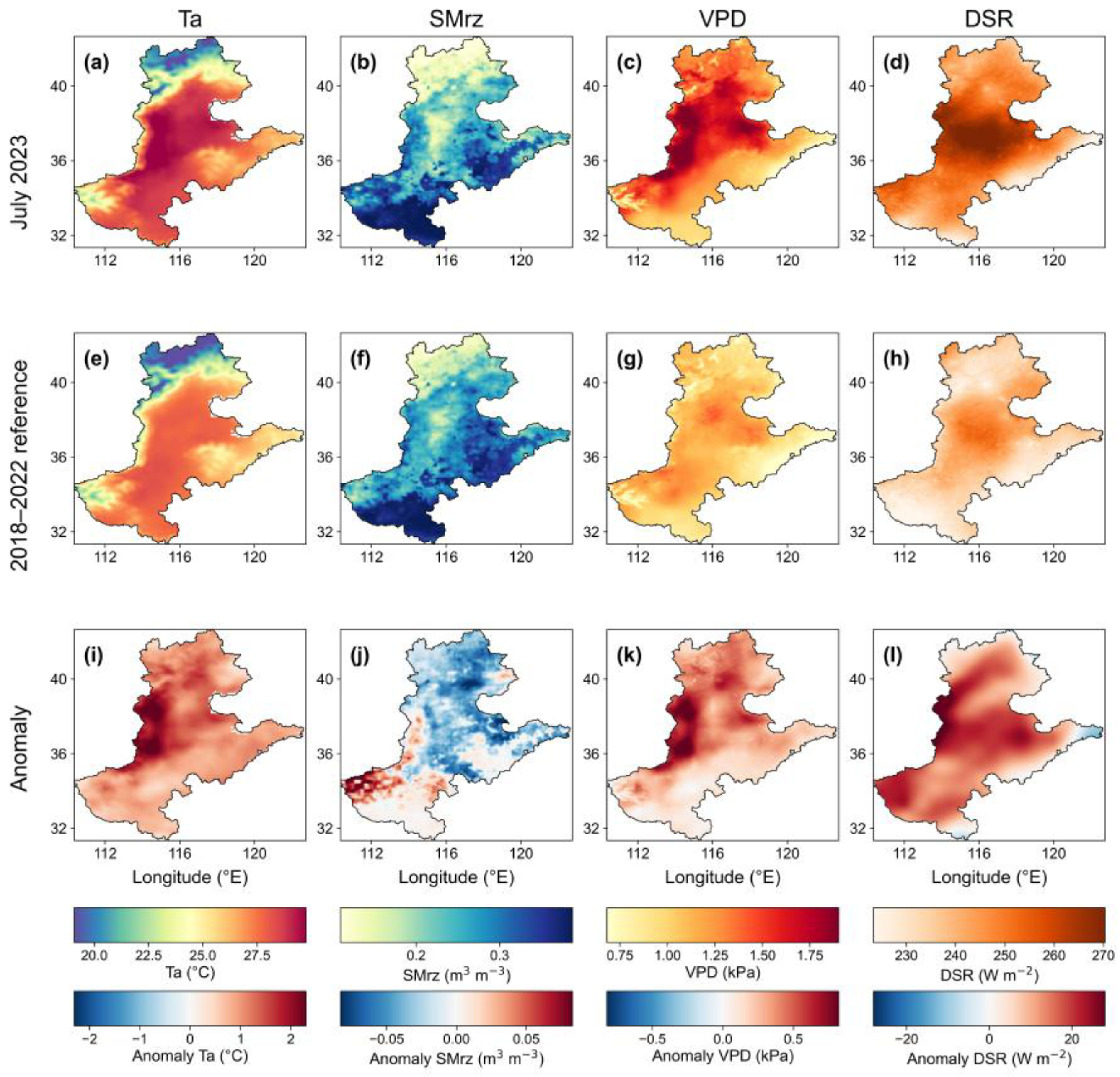
Relative to the 2018–2022 July reference, Ta was higher throughout the vegetated area; VPD and DSR were positive across 99.7% and 96.3% of vegetated pixels, respectively; and SMrz was negative across 65.9%, with localized positive anomalies embedded within the broader drying pattern (Figure 2a–l). The area-weighted mean anomalies were +1.1100 °C for Ta (95% CI: +1.0163 to +1.2082), −0.0147 m3 m−3 for SMrz (95% CI: −0.0213 to −0.0077), +0.3158 kPa for VPD (95% CI: +0.2724 to +0.3606), and +14.0699 W m−2 for DSR (95% CI: +12.5329 to +15.5089) (Table S4). The dominant signal was therefore widespread heat and atmospheric demand, while local root zone water availability varied substantially. This spatial decoupling creates a supply–demand gradient: the same atmospheric forcing can impose very different physiological stress where roots can or cannot meet evaporative demand [49,50,51]. Monsoon rainfall and irrigation likely contributed to the heterogeneous SMrz pattern [20,21], while peak-season water demand and crop phenology further differentiated exposure [22,23,24].
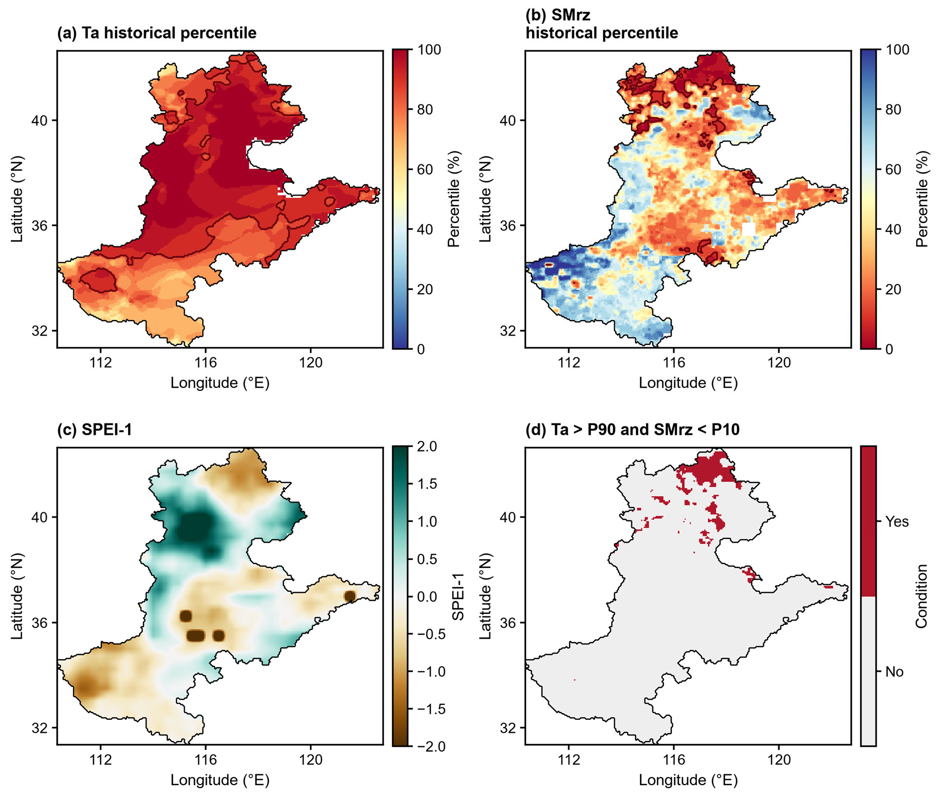
Percentile diagnostics confirmed that widespread atmospheric heat and local drought in root zone soil moisture were spatially decoupled. Ta exceeded the local July P90 threshold across 59.6% of vegetated pixels (Figure 3a); SMrz fell below the local P10 threshold across 7.9% (Figure 3b); SPEI-1 was ≤−1 in 6.5% (Figure 3c); and simultaneous Ta > P90 and SMrz < P10 covered 4.7% (Figure 3d). July 2023 was thus characterized by widespread heat exceedance with root zone soil drying concentrated in a smaller set of locations where local water supply was least able to offset atmospheric demand.
The same 2001–2022 pixel-specific thresholds revealed strong interannual contrasts within the recent period: during July 2018–2022, Ta > P90 coverage ranged from 0.0% to 58.5%, SMrz < P10 from 0.0% to 40.9%, and compound coverage from 0.0% to 29.1% (Table S7). Relative to the 2018–2022 June mean, the June 2023 Ta was near-neutral (−0.0365 °C) and SMrz slightly positive (+0.0042 m3 m−3), whereas VPD (+0.1809 kPa) and DSR (+14.6981 W m−2) were elevated. SPEI-1 ≤ −1 covered 54.2% of vegetated area (Table S8). During 2018–2023, 2023 was distinguished by its heat coverage rather than by the most extensive deficit in root zone soil moisture or compound coverage, providing a climate setting in which productivity losses could vary with local water supply.

3.2. Vegetation Productivity Loss During the Event

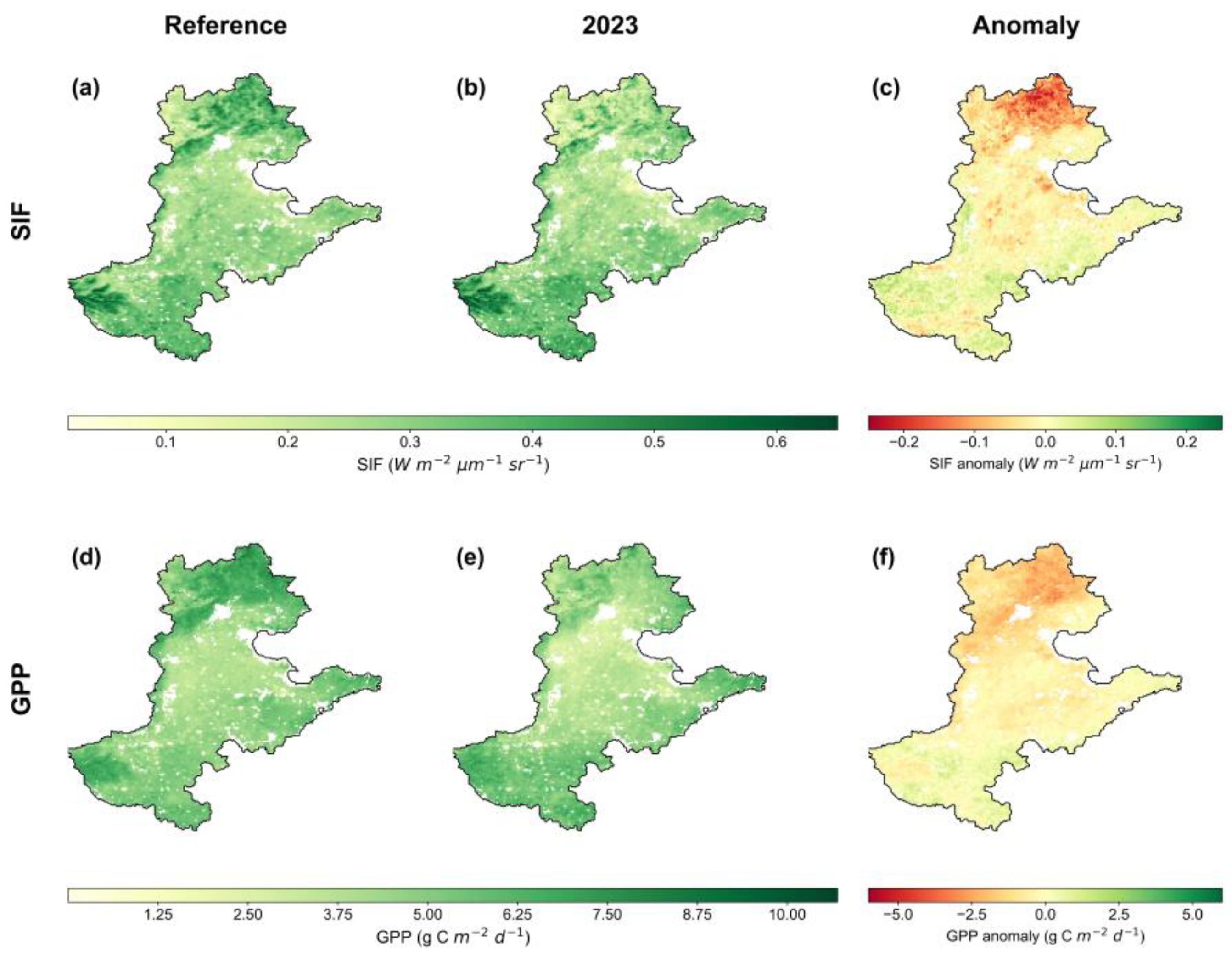
The atmospheric heat–demand pattern and heterogeneous SMrz anomalies shown in Figure 2 and Figure 3 were accompanied by a widespread but spatially uneven productivity decline. The reference and July 2023 fields retained similar broad gradients, yet anomaly maps showed extensive negative departures across the northern and central HHH Plain and smaller near-zero or positive areas farther south (Figure 4a–f). Area-weighted mean anomalies were −0.0129 W m−2 μm−1 sr−1 for SIF (95% CI: −0.0230 to −0.0035) and −0.4853 g C m−2 d−1 for GPP (95% CI: −0.6698 to −0.3057); negative anomalies occurred in 57.3% of vegetated pixels for SIF and 73.4% for GPP (Table S4). The agreement in sign and regional extent between the two products provides complementary evidence that the July climate configuration was associated with a broad productivity loss.
The spatial loss pattern follows the ecological logic of a supply–demand mismatch. Elevated Ta raises leaf energy load, and higher VPD increases evaporative demand and the atmospheric pressure deficit experienced by vegetation [5,51,52]. When water supply cannot meet that demand, stomatal closure restricts CO2 diffusion and carbon assimilation, while reduced SMrz further limits root water uptake, leaf hydration, and canopy conductance [7,49,50]. The spatial clustering of negative SIF and GPP anomalies is consistent with overlapping stresses, linking the environmental gradients in Figure 2 to the productivity gradients in Figure 4.
SIF and GPP agreed in their regional decline but differed in spatial detail (Figure 4c,f). GOSIF is reconstructed from OCO-2 SIF, MODIS reflectance, MERRA-2 PAR, air temperature, and VPD [13,53], whereas MODIS GPP uses a light use efficiency algorithm [35]. SIF is more directly related to photosynthetic apparatus function, while GPP is an algorithm-derived carbon flux estimate; their convergence therefore offers complementary evidence, while differences can reflect product resolution, screening, model structure, input datasets, and response times [54]. SMrz is not a direct GOSIF input, although GOSIF contains meteorological information relevant to interpreting their spatial agreement. Regional mean SIF anomalies were −0.01294 W m−2 μm−1 sr−1 relative to 2018–2022, +0.00945 relative to the raw 2001–2022 mean, and −0.02040 relative to the detrended 2001–2022 reference (Figure S1). Thus, the negative regional anomaly applies to the recent and detrended references. The recent and detrended standardized definitions identify 2833 and 3684 affected pixels, respectively, of which 85.6% and 87.8% recovered by October (Figure S2; Table S2). Similar recovery proportions coexist with a change in affected extent.
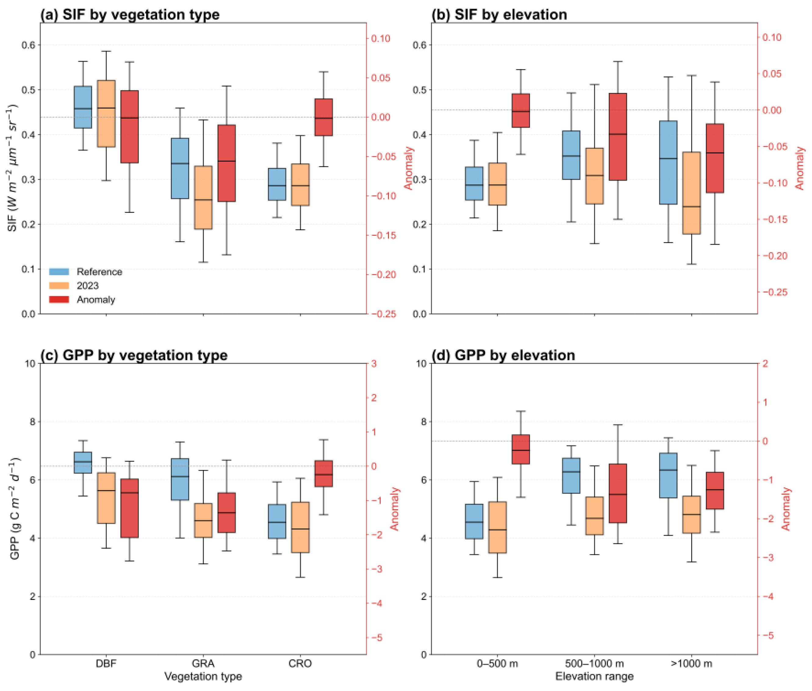
Vegetation type and elevation further organized the regional decline. SIF shifted most strongly downward for GRA, whose mean anomaly was −0.0583 W m−2 μm−1 sr−1 compared with −0.0109 for DBF and −0.0013 for CRO (Figure 5a). GPP showed the same broad ordering, with stronger losses in DBF and GRA than in CRO, although class separation was less distinct than for SIF (Figure 5c). The GRA–DBF SIF contrast was −0.0475 (95% CI: −0.0739 to −0.0138), and the GRA–CRO contrast was −0.0570 (95% CI: −0.0795 to −0.0318); both remained significant after Holm adjustment, whereas DBF and CRO did not differ significantly (Tables S4 and S5).
The pronounced GRA loss is consistent with the rapid sensitivity of exposed herbaceous canopies to short-term water limitation and atmospheric dryness [6,51]. Because GRA can overlap higher-elevation and less-irrigated settings, the observed contrast likely combines vegetation sensitivity with exposure and water access rather than reflecting a single trait. The smaller mean decline in CRO suggests that cropland responses are more complex than can be explained by climate drivers alone and may also involve crop phenology, irrigation timing, and field management practices. DBF results primarily represent the dominant deciduous broadleaf subtype, and their spatial heterogeneity is consistent with variation in rooting depth, stand structure, and local soil water storage, and with regional hydrothermal evidence and evidence of forest dryness [55].
Elevation revealed a matching vulnerability gradient. SIF distributions shifted farther downward above 1000 m than at lower elevations (Figure 5b), with mean anomalies of −0.0645 W m−2 μm−1 sr−1 above 1000 m and −0.0015 at 0–500 m. The contrast between the lowest and highest elevation classes was +0.0630 (95% CI: +0.0315 to +0.0921; Holm-adjusted p = 0.0001), whereas intermediate pairwise contrasts were not significant after adjustment (Tables S4 and S5). GPP was negative across all elevation classes but showed a less pronounced gradient (Figure 5d). The stronger high-elevation SIF loss is compatible with the differences in soil depth, water storage, exposure, and vegetation structure that also shape post-event recovery.
Taken together, Figure 2, Figure 3, Figure 4 and Figure 5 show that a modest regional mean concealed exposure-specific vulnerability: atmospheric demand was widespread, but local water supply and landscape setting were associated with where productivity declined most strongly. The alignment of the largest July losses in GRA and above 1000 m with their subsequent recovery patterns in Section 3.3 points to initial disturbance severity as an important dimension of the recovery trajectory.

3.3. Recovery of Pixels with SIF Declines

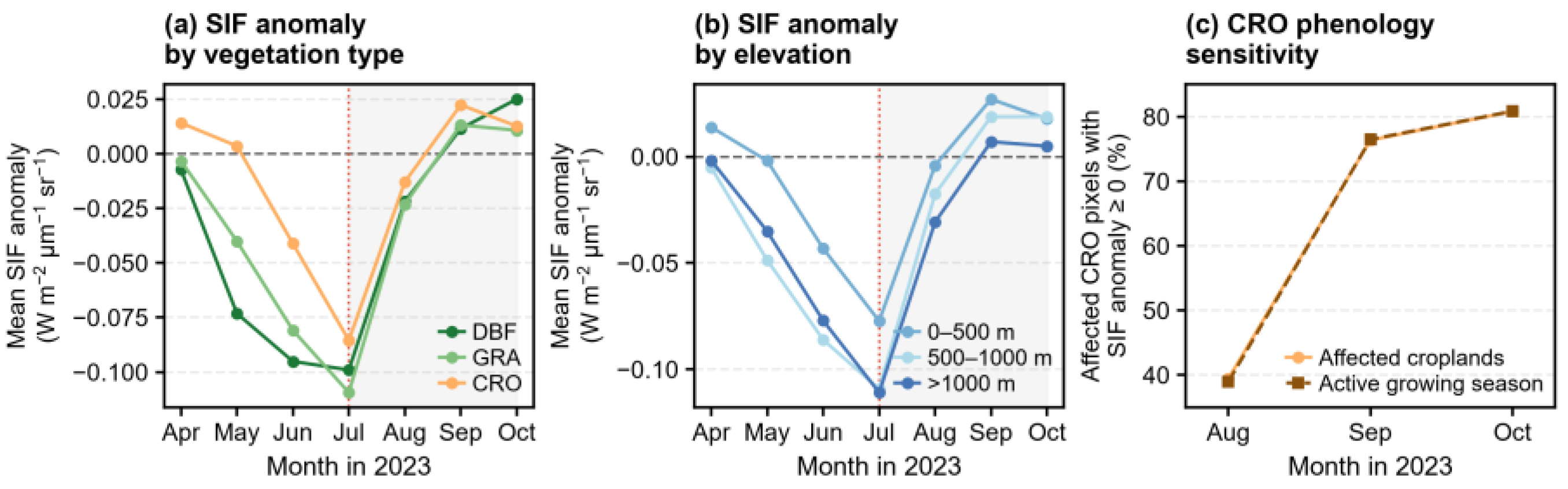
The April–October trajectories of the July-affected pixels differed before the event but converged in a pronounced midsummer decline (Figure 6a,b). For DBF, the mean SIF anomaly decreased from −0.0073 W m−2 μm−1 sr−1 in April to −0.0951 in June and reached −0.0990 in July, whereas GRA reached −0.1094 in July after progressively declining from April. CRO changed from a positive anomaly in April to −0.0411 in June and −0.0855 in July (Figure 6a). All three classes remained negative in August, crossed above zero in September, and remained positive in October (Figure 6a). Across elevation classes, July was the lowest point, with mean anomalies of −0.0773, −0.1092, and −0.1109 W m−2 μm−1 sr−1 at 0–500 m, 500–1000 m, and >1000 m, respectively; all three means became positive by September (Figure 6b).
Among affected CRO pixels, 39.4% had a non-negative SIF anomaly in August, increasing to 76.4% in September and 80.8% in October (Figure 6c). Restricting the calculation to MCD12Q2 pixels in the active growing season produced 38.9%, 76.5%, and 80.9%, respectively, with a maximum difference of only 0.5 percentage points (Figure 6c). The close trajectories show limited sensitivity to this CRO seasonal filter without excluding other phenological influences. The earlier negative DBF and GRA anomalies indicate antecedent seasonal variability in the affected pixels.
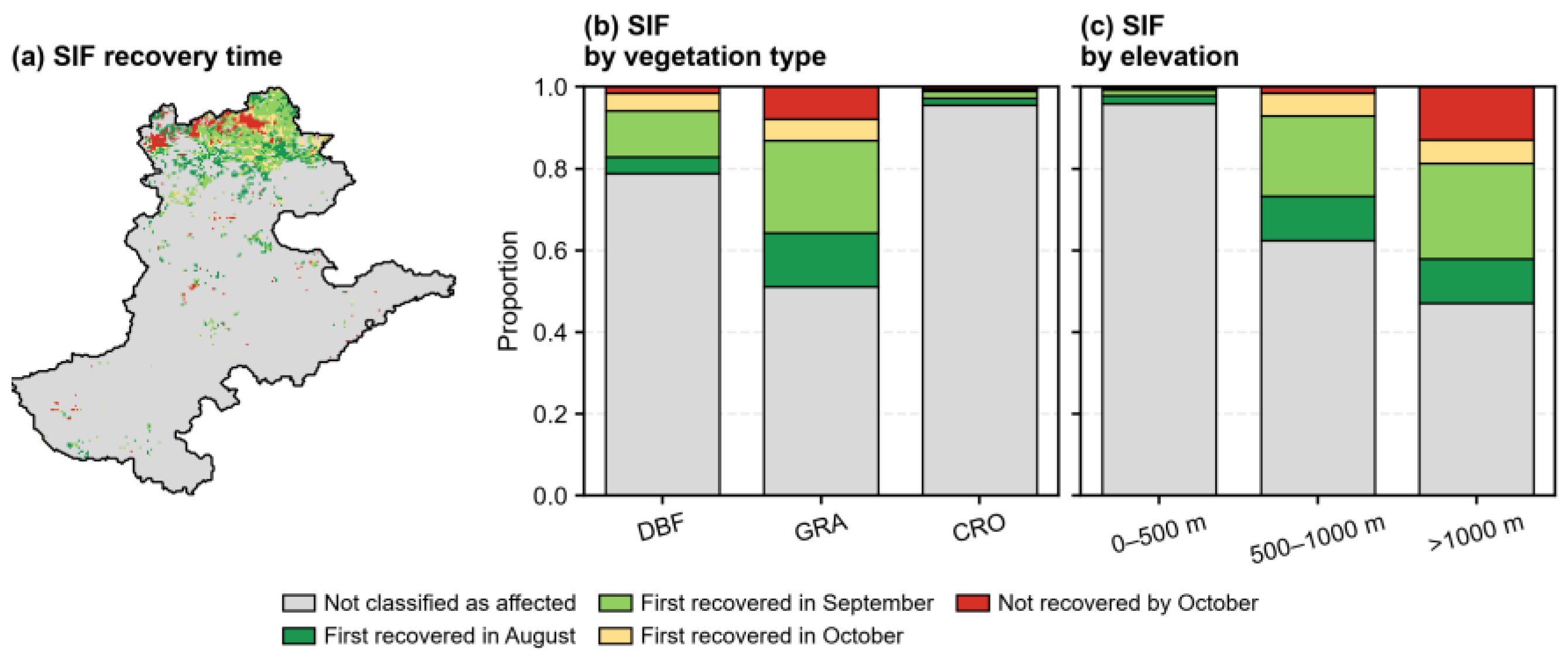
Recovery timing varied markedly across space and strata. The recovery status map shows a patchwork of recovery months and unrecovered pixels, with the largest coherent concentrations of affected pixels in the northern plain (Figure 7a). Among affected pixels, 19.1% of DBF, 26.9% of GRA, and 39.4% of CRO first recovered in August; cumulative October recovery reached 93.3%, 84.0%, and 87.9%, respectively (Figure 7b). By elevation, 48.1%, 28.9%, and 20.5% of affected pixels at 0–500 m, 500–1000 m, and >1000 m first recovered in August, while cumulative October proportions were 90.5%, 96.1%, and 75.6% (Figure 7c). Across all 2833 affected pixels, 85.6% reached a non-negative anomaly at least once by October.
The >1000 m class therefore combined the larger July loss with the slowest and least complete recovery, whereas lower-elevation pixels recovered more rapidly. A larger initial deficit can lengthen return to the reference state, while localized rainfall and root zone soil moisture recharge can generate a pixel-scale mosaic, as shown in Figure 7a [6,7,8]. Similar post-drought recovery variability occurs across bioclimatic settings [32]. The alignment of July severity in Figure 5b, October recovery in Figure 7c, and the importance of initial July loss in Section 3.4 supports initial-state dependence in the recovery trajectory. Differences among vegetation classes, including lower cumulative October recovery for GRA than for DBF and the rapid CRO rebound, may additionally reflect crop type, phenology, irrigation, and management [55,56].

3.4. Environmental Associations with SIF Decline and Recovery

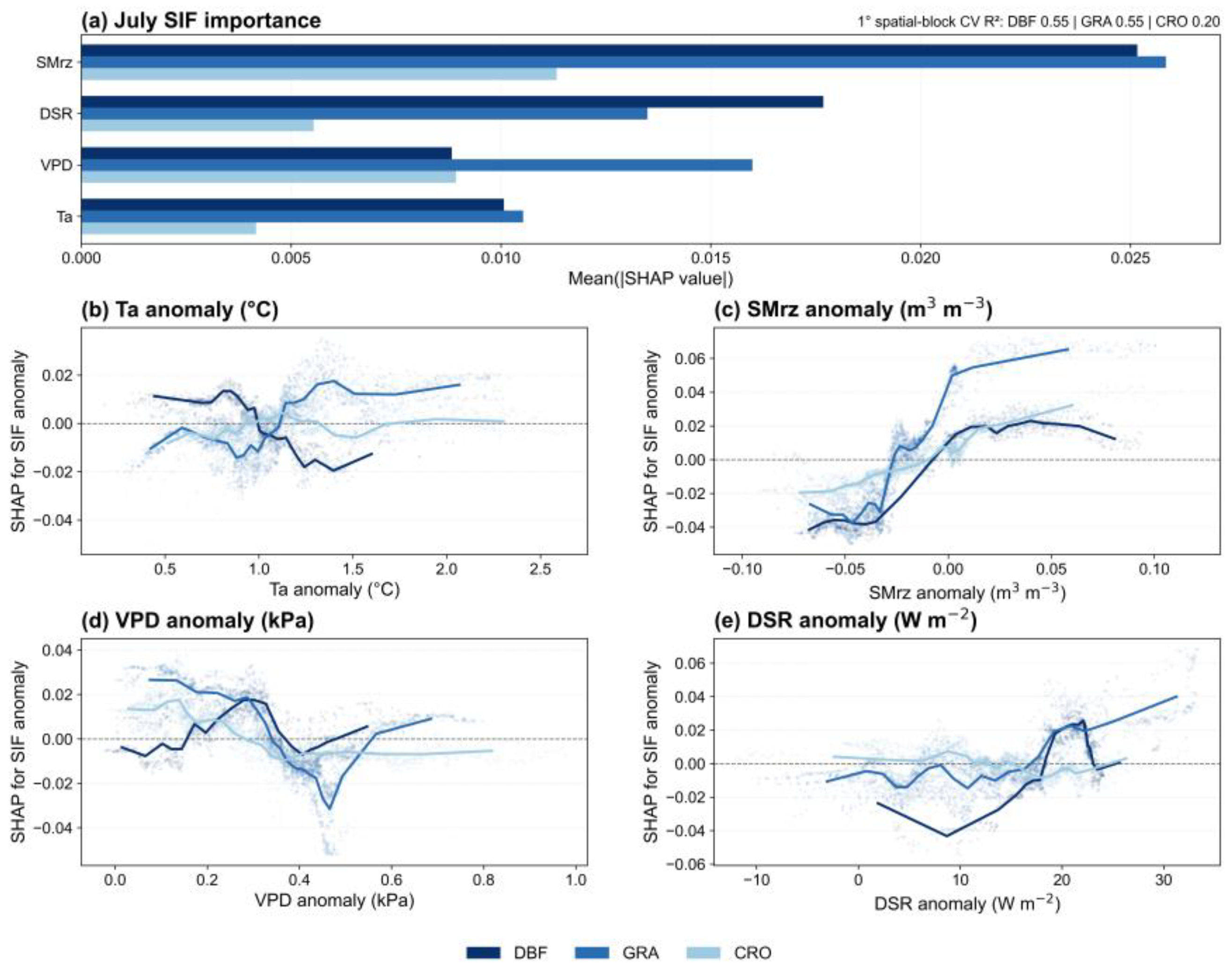
The July models point to coupled constraints from root zone soil moisture and atmospheric conditions rather than a single isolated predictor. SMrz had the largest individual mean absolute SHAP value for DBF, GRA, and CRO, accounting for 40.8%, 39.2%, and 37.8% of importance within each model, respectively (Figure 8a). Its response direction was also the most consistent: increasingly negative SMrz anomalies were associated with negative SHAP contributions, followed by positive contributions as SMrz approached or exceeded its reference value (Figure 8c). Ta, VPD, and DSR responses were nonlinear and differed among vegetation classes (Figure 8b,d,e). OOF R2 values under spatial block validation were 0.550 for DBF, 0.552 for GRA, and 0.205 for CRO (Figure 8a; Table S6), indicating moderate generalization for DBF and GRA but weak predictability using climate variables alone for CRO.
The common SMrz response is consistent with the roles of root zone water availability in leaf hydration, stomatal regulation, and light use efficiency during hot and dry conditions [7,49,50]. Its agreement across vegetation classes connects the localized SMrz drying in Figure 2j with the class-specific losses in Figure 5 and is consistent with water limitation across contrasting covers and variation in local exposure and water access.
The combined contribution of Ta, VPD, and DSR was comparable to that of SMrz. Correlations between Ta and VPD were 0.881 for DBF, 0.907 for GRA, and 0.945 for CRO, and the largest VIF was 9.69 (Figure S3; Table S3). Together, Ta, VPD, and DSR represented 47.9%, 48.7%, and 52.6% of grouped importance for DBF, GRA, and CRO, compared with 52.1%, 51.3%, and 47.4% for SMrz (Figure S4). Thus, the individual SMrz ranking and the similar contributions of these predictor sets support the interpretation of coupled constraints from root zone soil moisture and atmospheric demand, rather than a separable hierarchy of independent controls.
CRO illustrates why buffering and predictability need not coincide. Its weaker July OOF R2 indicates that climate variables explain only part of crop SIF variability; crop type, cultivar, planting date, irrigation timing and intensity, and management can decouple field responses from regional Ta, SMrz, VPD, and DSR. Filtering to the active growing season changed monthly recovery proportions by no more than 0.5 percentage points, while phenology variables increased overall recovery OOF R2 from 0.486 to 0.501 (Table S6). Managed cropland can therefore show a relatively small regional mean loss and rapid recovery while remaining difficult for a model using climate variables alone to predict at field scale.
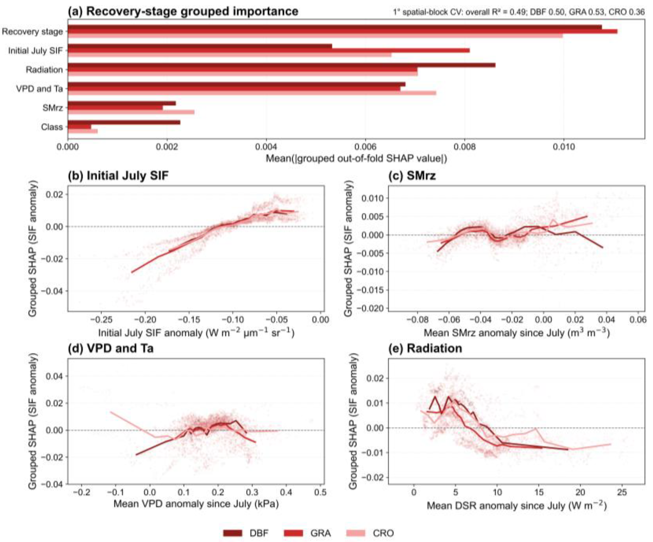
Recovery heterogeneity was jointly associated with seasonal stage, initial disturbance, and post-event environmental trajectories. Recovery stage contributed 30.8% of grouped out-of-fold SHAP importance, followed by initial July loss (21.5%), current DSR and its mean since July (20.4%), current Ta and VPD and their means since July (19.6%), current SMrz and its mean since July (5.9%), and vegetation class (1.8%) (Figure 9a). The model explained 48.6% of out-of-fold variation overall, with OOF R2 values of 0.499 for DBF, 0.533 for GRA, and 0.362 for CRO (Figure 9a; Table S6). More negative initial July anomalies were associated with negative SHAP contributions during recovery (Figure 9b), mean SMrz since July shifted from negative to mostly positive contributions as its mean anomaly approached zero (Figure 9c), and SHAP responses to mean VPD and DSR anomalies since July were nonlinear and differed among vegetation classes (Figure 9d,e).
The relationship between initial July loss and SHAP contributions in Figure 9b suggests persistence of initial SIF differences: a larger July deficit was associated with lower predicted SIF anomalies during recovery. The response to mean SMrz since July is consistent with improvement as root zone water conditions recovered. The nonmonotonic response to temperature and atmospheric demand indicates that these conditions were related to recovery heterogeneity across the observed range, while DSR contributions changed from positive to negative at higher mean anomalies since July, consistent with a balance between energy supply for photosynthesis and radiation-associated thermal or evaporative stress [57,58]. Recovery was therefore associated with both the post-event climate trajectory and the initial July SIF state.
CRO again combined relatively rapid broad recovery with weaker model transfer than DBF and GRA (Figure 9a). The comparison restricted to the active growing season produced similar monthly recovery proportions, while adding phenology variables changed overall OOF R2 from 0.486 to 0.501 and increased OOF R2 for the model fitted only to CRO from 0.286 to 0.309 (Table S6) [59]. These similar active-season fractions show limited sensitivity to this filter; differences in crop calendars, irrigation, and management among fields remain unresolved.
These XGBoost–SHAP results describe spatial associations among pixels in July and associations across pixels and months during August–October within the specified products and predictor sets. GOSIF uses meteorological inputs in its construction [13], so its relationships with Ta, VPD, and DSR can contain both vegetation responses and patterns inherited from the product model. Correlations, VIFs, and grouped SHAP diagnose shared information among predictors; they do not separate this product dependence from vegetation responses. Current SMrz and its mean since July had a correlation of 0.928 and current Ta and its mean since July 0.877, and VIFs reached 29.4 for current Ta (Figure S3; Table S3). Monthly means can smooth brief heat peaks and rapid soil drying, and can combine stress, rainfall, and recovery within one observation. They therefore obscure the onset, peak magnitude, duration, and ordering of short-lived events and SIF responses. Daily or sub-monthly observations can help distinguish heat and water deficit onset, rainfall or irrigation pulses, and the delay before photosynthetic recovery. June 2023 conditions describe the period before the July event; their lagged effect on July SIF was not estimated [60]. Seasonal changes in DBF and GRA may affect SIF zero crossing, and similar CRO active-season fractions do not exclude all phenological influences. Recovery proportions and speed differences are reported without confidence intervals or significance tests. Future studies could combine irrigation, crop calendar, and soil profile information with higher-frequency observations. Products such as hourly GPP (EGO) and complementary vegetation indices (kNDVI) offer additional perspectives, although their sampling and product dependence also require evaluation [61,62].

4. Conclusions

This study investigated vegetation productivity responses associated with the July 2023 hot–dry event across the Huang–Huai–Hai Plain using GOSIF as the primary productivity indicator, complemented by MODIS GPP, with Ta, SMrz, VPD, and DSR as explanatory variables and XGBoost–SHAP to examine environmental associations. The event coincided with elevated Ta, VPD, and DSR and reduced SMrz, together with widespread negative anomalies in satellite-observed GOSIF and GPP. Productivity losses showed pronounced spatial heterogeneity: GRA exhibited a larger mean SIF decline than DBF and CRO, and areas above 1000 m showed greater losses than areas at 0–500 m, with these contrasts supported by bootstrap estimates using spatial blocks. Among the 2833 pixels identified by the 2018–2022 standardized anomaly criterion zi ≤ −1.5, 85.6% returned to non-negative SIF anomalies by October, whereas the corresponding recovery proportion above 1000 m was 75.6%. Recovery therefore remained incomplete for a subset of GRA, CRO, and high-elevation pixels. Validation using spatial blocks supported the July DBF and GRA models more strongly than the CRO model, and the recovery model achieved an overall OOF R2 of 0.486 with weaker CRO generalization. Within the July models, SMrz carried the largest individual predictive association, although the combined contribution of Ta, VPD, and DSR carried comparable information. Within the recovery model, recovery stage, initial July loss, radiation, temperature, and atmospheric demand each contained substantial predictive information. These model results describe the environmental information associated with July loss and subsequent recovery. The low CRO OOF R2 indicates that climate predictors alone cannot adequately explain SIF spatial variability in croplands; future work may further consider irrigation, crop type, planting date, crop calendars, and management data. Together, the results provide a spatially validated characterization of productivity loss, recovery, and associated environmental heterogeneity during the July 2023 hot–dry event on the HHH Plain.

Supplementary Materials

The following supporting information can be downloaded at: https://www.mdpi.com/article/10.3390/land15091701/s1, Figure S1. Sensitivity of July 2023 GOSIF anomalies to recent, raw long-term, and detrended long-term reference definitions. Panel (a) shows the 2018–2022 anomaly; panel (b) the raw 2001–2022 anomaly; panel (c) the deviation from the 2001–2022 trend prediction; and panel (d) the detrended residual standardized by its historical residual standard deviation. Figure S2. Sensitivity of the affected-pixel extent to the reference-period standardization. The main analysis uses the non-detrended 2018–2022 standardized anomaly (zi ≤ −1.5); the comparison shows only the 2001–2022 detrended standardized sensitivity. Figure S3. Pearson correlation matrices for environmental predictors in the three July models and the recovery model. Panels (a–c) show July correlations for DBF, GRA, and CRO; panel (d) shows correlations among current and mean-since-July predictors during recovery. SMrz denotes the GLEAM root-zone soil moisture variable used in the corresponding analysis. Figure S4. Grouped SHAP importance for the three July models and the recovery model. Panel (a) compares the combined contribution of Ta, VPD, and DSR with that of SMrz in July; panel (b) summarizes grouped out-of-fold importance in the recovery model. Recovery stage and vegetation class provide contextual information and are not independently identified mechanisms. Figure S5. Area weighted July 2023 SIF and GPP anomalies with 95% confidence intervals from bootstrap resampling using 1° × 1° spatial blocks. Panels (a) and (b) show vegetation type and elevation class SIF anomalies; panels (c) and (d) show corresponding GPP anomalies. Table S1. Comparison of 2018–2022 and 2001–2022 reference-period environmental anomalies and spatial consistency. The SMrz row uses the GLEAM4.2a data for the long-term sensitivity analysis and is consistent with the product used for the main analysis in Table S4. Table S2. Sensitivity of affected-pixel identification and recovery to the reference period. The main analysis uses the non-detrended 2018–2022 standardized anomaly (zi ≤ −1.5); the comparison reports only the 2001–2022 detrended standardized sensitivity. Table S3. VIF values for individual predictors in the July models and recovery model. N and spatial blocks are the valid samples for each model. The recovery entries were traced to the dataset of 8442 records from 2814 pixels spanning 51 spatial blocks. VIF values diagnose predictor collinearity and are not effect estimates. Table S4. Area-weighted July 2023 anomalies and 95% confidence intervals by variable, vegetation type, and elevation class. Estimates use bootstrap resampling using 1° × 1° spatial blocks with 5000 replicates and cosine-latitude weights. The SMrz values use the processed GLEAM4.2a data used in the main anomaly and model analyses. Table S5. Pairwise contrasts of area-weighted July 2023 GOSIF anomalies. Differences are Group 1 minus Group 2. Estimates and 95% CIs use 5000 resamples of 1° × 1° spatial blocks with cosine-latitude weights; two-sided raw p-values use the bootstrap-difference normal approximation and are Holm-adjusted within the GOSIF comparison family. Table S6. XGBoost model performance evaluated with five-fold cross-validation using 1° × 1° spatial blocks. N is the number of valid records; for recovery models, the number of unique affected pixels is also given. DBF, GRA, and CRO subgroup rows are held-out subset scores from the same recovery model rather than separately fitted models, so subgroup in-sample R2 was not calculated. OOF denotes out-of-fold performance; RMSE and MAE are in SIF anomaly units (W m−2 μm−1 sr−1). Table S7. July heat and drought diagnostics for 2018–2023 using the same pixel-specific 2001–2022 July thresholds. Percentages are cosine-latitude area-weighted fractions of vegetated pixels. The 2018–2022 rows diagnose interannual conditions within the recent period used as the primary reference; 2023 is included for event context. Table S8. June 2023 conditions before the July event. Ta, SMrz, VPD, and DSR anomalies are derived relative to the 2018–2022 June mean; SPEI-1 is reported on its native standardized scale.

Author Contributions

F.Q.: writing—original draft, visualization, validation, methodology, investigation, formal analysis, data curation. X.L. (Xi Liu): writing—review and editing, visualization, validation, methodology, conceptualization. X.L. (Xing Li): writing—review and editing, supervision, funding acquisition. All authors have read and agreed to the published version of the manuscript.

Funding

This study was supported by the Fundamental Research Funds for Central Universities, Sun Yat-sen University (Grant No. 25hytd002) and the National Natural Science Foundation of China (Grant No. 42401412).

Data Availability Statement

The GOSIF product is available from the University of New Hampshire Global Ecology Group Data Repository (https://globalecology.unh.edu/data/GOSIF.html (accessed on 9 September 2026)). MOD17A2HGF v6.1, MCD12Q1 v6.1, MCD12Q2 v6.1, and SRTMGL1 v3 are available from NASA Earthdata (https://www.earthdata.nasa.gov/). ERA5-Land is available from the Copernicus Climate Data Store [36], and ERA5–Drought SPEI-1 is available from the ECMWF-hosted data store [39]. GLEAM4.2a SMrz data are available from the GLEAM data portal (https://www.gleam.eu/) [37]. TerraClimate is available from the Climatology Lab (https://www.climatologylab.org/). Processed data and the analysis code are available from the corresponding author upon reasonable request.

Conflicts of Interest

The authors declare no conflicts of interest.

References

  1. Zhou, S.; Zhang, Y.; Park Williams, A.; Gentine, P. Projected increases in intensity, frequency, and terrestrial carbon costs of compound drought and aridity events. Sci. Adv. 2019, 5, eaau5740. [Google Scholar] [CrossRef] [Scilit] [PubMed]
  2. Trenberth, K.E.; Dai, A.; van der Schrier, G.; Jones, P.D.; Barichivich, J.; Briffa, K.R.; Sheffield, J. Global warming and changes in drought. Nat. Clim. Change 2014, 4, 17–22. [Google Scholar] [CrossRef] [Scilit]
  3. Zscheischler, J.; Westra, S.; van den Hurk, B.J.J.M.; Seneviratne, S.I.; Ward, P.J.; Pitman, A.; AghaKouchak, A.; Bresch, D.N.; Leonard, M.; Wahl, T.; et al. Future climate risk from compound events. Nat. Clim. Change 2018, 8, 469–477. [Google Scholar] [CrossRef] [Scilit]
  4. Zscheischler, J.; Mahecha, M.D.; von Buttlar, J.; Harmeling, S.; Jung, M.; Rammig, A.; Randerson, J.T.; Schölkopf, B.; Seneviratne, S.I.; Tomelleri, E.; et al. A few extreme events dominate global interannual variability in gross primary production. Environ. Res. Lett. 2014, 9, 035001. [Google Scholar] [CrossRef] [Scilit]
  5. Grossiord, C.; Buckley, T.N.; Cernusak, L.A.; Novick, K.A.; Poulter, B.; Siegwolf, R.T.W.; Sperry, J.S.; McDowell, N.G. Plant responses to rising vapor pressure deficit. New Phytol. 2020, 226, 1550–1566. [Google Scholar] [CrossRef] [Scilit] [PubMed]
  6. Li, W.; Pacheco-Labrador, J.; Migliavacca, M.; Miralles, D.; Hoek van Dijke, A.; Reichstein, M.; Forkel, M.; Zhang, W.; Frankenberg, C.; Panwar, A.; et al. Widespread and complex drought effects on vegetation physiology inferred from space. Nat. Commun. 2023, 14, 4640. [Google Scholar] [CrossRef] [Scilit] [PubMed]
  7. Stocker, B.D.; Zscheischler, J.; Keenan, T.F.; Prentice, I.C.; Peñuelas, J.; Seneviratne, S.I. Quantifying soil moisture impacts on light use efficiency across biomes. New Phytol. 2018, 218, 1430–1449. [Google Scholar] [CrossRef] [Scilit] [PubMed]
  8. Stocker, B.D.; Zscheischler, J.; Keenan, T.F.; Prentice, I.C.; Seneviratne, S.I.; Peñuelas, J. Drought impacts on terrestrial primary production underestimated by satellite monitoring. Nat. Geosci. 2019, 12, 264–270. [Google Scholar] [CrossRef] [Scilit]
  9. AghaKouchak, A.; Farahmand, A.; Melton, F.S.; Teixeira, J.; Anderson, M.C.; Wardlow, B.D.; Hain, C.R. Remote sensing of drought: Progress, challenges and opportunities. Rev. Geophys. 2015, 53, 452–480. [Google Scholar] [CrossRef] [Scilit]
  10. Sun, Y.; Frankenberg, C.; Wood, J.D.; Schimel, D.S.; Jung, M.; Guanter, L.; Drewry, D.T.; Verma, M.; Porcar-Castell, A.; Griffis, T.J.; et al. OCO-2 advances photosynthesis observation from space via solar-induced chlorophyll fluorescence. Science 2017, 358, eaam5747. [Google Scholar] [CrossRef] [Scilit] [PubMed]
  11. Porcar-Castell, A.; Tyystjärvi, E.; Atherton, J.; van der Tol, C.; Flexas, J.; Pfündel, E.E.; Moreno, J.; Frankenberg, C.; Berry, J.A. Linking chlorophyll a fluorescence to photosynthesis for remote sensing applications: Mechanisms and challenges. J. Exp. Bot. 2014, 65, 4065–4095. [Google Scholar] [CrossRef] [Scilit] [PubMed]
  12. Li, X.; Xiao, J.; He, B.; Altaf Arain, M.; Beringer, J.; Desai, A.R.; Emmel, C.; Hollinger, D.Y.; Krasnova, A.; Mammarella, I.; et al. Solar-induced chlorophyll fluorescence is strongly correlated with terrestrial photosynthesis for a wide variety of biomes: First global analysis based on OCO-2 and flux tower observations. Glob. Change Biol. 2018, 24, 3990–4008. [Google Scholar] [CrossRef] [Scilit] [PubMed]
  13. Li, X.; Xiao, J. A global, 0.05-degree product of solar-induced chlorophyll fluorescence derived from OCO-2, MODIS, and reanalysis data. Remote Sens. 2019, 11, 517. [Google Scholar] [CrossRef] [Scilit]
  14. Zhang, Y.; Joiner, J.; Alemohammad, S.H.; Zhou, S.; Gentine, P. A global spatially contiguous solar-induced fluorescence (CSIF) dataset using neural networks. Biogeosciences 2018, 15, 5779–5800. [Google Scholar] [CrossRef] [Scilit]
  15. Zhang, Y.; Liu, F.; Liu, T.; Chen, C.; Lu, Z. Characteristics of vegetation photosynthesis under flash droughts in the major agricultural areas of southern China. Atmosphere 2024, 15, 886. [Google Scholar] [CrossRef] [Scilit]
  16. Klein, C.; Hänchen, L.; Potter, E.R.; Junquas, C.; Harris, B.L.; Maussion, F. Untangling the importance of dynamic and thermodynamic drivers for wet and dry spells across the Tropical Andes. Environ. Res. Lett. 2023, 18, 034002. [Google Scholar] [CrossRef] [Scilit]
  17. Qiu, R.; Li, X.; Han, G.; Xiao, J.; Ma, X.; Gong, W. Monitoring drought impacts on crop productivity of the U.S. Midwest with solar-induced fluorescence: GOSIF outperforms GOME-2 SIF and MODIS NDVI, EVI, and NIRv. Agric. For. Meteorol. 2022, 323, 109038. [Google Scholar] [CrossRef] [Scilit]
  18. Wang, H.; Zhang, Z.; Wu, X.; Xu, J.; Han, J.; Zhuang, H.; Li, S.; Song, J.; Cheng, F.; Piao, S.; et al. Spatially explicit temperature optima improve climate impact assessment of global crop productivity. Nat. Commun. 2026. [Google Scholar] [CrossRef] [Scilit] [PubMed]
  19. Jiang, Y.; Shi, H.; Yang, X.; Wen, Z.; Wu, Y.; Wang, Y.; Duan, G.; Gormley, A.G.; Yang, G.; Li, J. Tracking drought dynamics on China’s Loess Plateau with the rapid change index of solar-induced chlorophyll fluorescence. Int. J. Digit. Earth 2025, 18, 2473128. [Google Scholar] [CrossRef] [Scilit]
  20. Liu, Y.; Wang, E.; Yang, X.; Wang, J. Contributions of climatic and crop varietal changes to crop production in the North China Plain, since 1980s. Glob. Change Biol. 2010, 16, 2287–2299. [Google Scholar] [CrossRef] [Scilit]
  21. Xiao, D.; Tao, F.; Liu, Y.; Shi, W.; Wang, M.; Liu, F.; Zhang, S.; Zhu, Z. Observed changes in winter wheat phenology in the North China Plain for 1981–2009. Int. J. Biometeorol. 2013, 57, 275–285. [Google Scholar] [CrossRef] [Scilit] [PubMed]
  22. Chen, W.; Yao, R.; Sun, P.; Zhang, Q.; Singh, V.P.; Sun, S.; AghaKouchak, A.; Ge, C.; Yang, H. Drought risk assessment of winter wheat at different growth stages in Huang-Huai-Hai Plain based on nonstationary standardized precipitation evapotranspiration index and crop coefficient. Remote Sens. 2024, 16, 1625. [Google Scholar] [CrossRef] [Scilit]
  23. Chen, G.; Li, K.; Gu, H.; Cheng, Y.; Xue, D.; Jia, H.; Du, Z.; Li, Z. Climatic challenges in the growth cycle of winter wheat in the Huang-Huai-Hai Plain: New perspectives on high-temperature–drought and low-temperature–drought compound events. Atmosphere 2024, 15, 747. [Google Scholar] [CrossRef] [Scilit]
  24. Zhao, J.; Peng, H.; Yang, J.; Huang, R.; Huo, Z.; Ma, Y. Response of winter wheat to different drought levels based on Google Earth Engine in the Huang-Huai-Hai Region, China. Agric. Water Manag. 2024, 292, 108662. [Google Scholar] [CrossRef] [Scilit]
  25. Wang, Q.; Liao, Z.; Zhai, P.; Peng, Y. Record-breaking heatwave in North China during the midsummer of 2023. Int. J. Climatol. 2024, 44, 4206–4218. [Google Scholar] [CrossRef] [Scilit]
  26. Gui, K.; Zhou, T. Soil moisture feedback amplified the earlier onset of the record-breaking three-day consecutive heatwave in 2023 in North China. Earth’s Future 2025, 13, e2024EF005561. [Google Scholar] [CrossRef] [Scilit]
  27. Qian, C.; Ye, Y.; Jiang, J.; Zhong, Y.; Zhang, Y.; Pinto, I.; Huang, C.; Li, S.; Wei, K. Rapid attribution of the record-breaking heatwave event in North China in June 2023 and future risks. Environ. Res. Lett. 2024, 19, 014028. [Google Scholar] [CrossRef] [Scilit]
  28. Yang, L.; Song, J.; Hu, F.; Han, L.; Wang, J. Monitoring the impact of heat damage on summer maize on the Huanghuaihai Plain, China. Remote Sens. 2023, 15, 2773. [Google Scholar] [CrossRef] [Scilit]
  29. Liu, Y.; Long, H.; Li, T.; Tu, S. Land use transitions and their effects on water environment in Huang-Huai-Hai Plain, China. Land Use Policy 2015, 47, 293–301. [Google Scholar] [CrossRef] [Scilit]
  30. Kang, S.; Eltahir, E.A.B. North China Plain threatened by deadly heatwaves due to climate change and irrigation. Nat. Commun. 2018, 9, 2894. [Google Scholar] [CrossRef] [Scilit] [PubMed]
  31. Fan, Y.; Miguez-Macho, G.; Jobbágy, E.G.; Jackson, R.B.; Otero-Casal, C. Hydrologic regulation of plant rooting depth. Proc. Natl. Acad. Sci. USA 2017, 114, 10572–10577. [Google Scholar] [CrossRef] [Scilit] [PubMed]
  32. Jiao, T.; Williams, C.A.; De Kauwe, M.G.; Schwalm, C.R.; Medlyn, B.E. Patterns of post-drought recovery are strongly influenced by drought duration, frequency, post-drought wetness, and bioclimatic setting. Glob. Change Biol. 2021, 27, 4630–4643. [Google Scholar] [CrossRef] [Scilit] [PubMed]
  33. Friedl, M.; Sulla-Menashe, D. MCD12Q1 MODIS/Terra+Aqua Land Cover Type Yearly L3 Global 500 m SIN Grid V061 [Dataset]; NASA EOSDIS Land Processes Distributed Active Archive Center: Sioux Falls, SD, USA, 2022. [CrossRef]
  34. Running, S.; Zhao, M. MOD17A2HGF MODIS/Terra Gross Primary Productivity Gap-Filled 8-Day L4 Global 500 m SIN Grid V061 [Dataset]; NASA EOSDIS Land Processes Distributed Active Archive Center: Sioux Falls, SD, USA, 2021. [CrossRef]
  35. Zhao, M.; Heinsch, F.A.; Nemani, R.R.; Running, S.W. Improvements of the MODIS terrestrial gross and net primary production global data set. Remote Sens. Environ. 2005, 95, 164–176. [Google Scholar] [CrossRef] [Scilit]
  36. Muñoz-Sabater, J.; Dutra, E.; Agustí-Panareda, A.; Albergel, C.; Arduini, G.; Balsamo, G.; Boussetta, S.; Choulga, M.; Harrigan, S.; Hersbach, H.; et al. ERA5-Land: A state-of-the-art global reanalysis dataset for land applications. Earth Syst. Sci. Data 2021, 13, 4349–4383. [Google Scholar] [CrossRef] [Scilit]
  37. Miralles, D.G.; Bonte, O.; Koppa, A.; Baez-Villanueva, O.M.; Tronquo, E.; Zhong, F.; Beck, H.E.; Hulsman, P.; Dorigo, W.; Verhoest, N.E.C.; et al. GLEAM4: Global land evaporation and soil moisture dataset at 0.1° resolution from 1980 to near present. Sci. Data 2025, 12, 416. [Google Scholar] [CrossRef] [Scilit] [PubMed]
  38. Abatzoglou, J.T.; Dobrowski, S.Z.; Parks, S.A.; Hegewisch, K.C. TerraClimate, a high-resolution global dataset of monthly climate and climatic water balance from 1958–2015. Sci. Data 2018, 5, 170191. [Google Scholar] [CrossRef] [Scilit] [PubMed]
  39. Keune, J.; Di Giuseppe, F.; Barnard, C.; Damasio da Costa, E.; Wetterhall, F. ERA5–Drought: Global drought indices based on ECMWF reanalysis. Sci. Data 2025, 12, 616. [Google Scholar] [CrossRef] [Scilit] [PubMed]
  40. Vicente-Serrano, S.M.; Beguería, S.; López-Moreno, J.I. A Multiscalar Drought Index Sensitive to Global Warming: The Standardized Precipitation Evapotranspiration Index. J. Clim. 2010, 23, 1696–1718. [Google Scholar] [CrossRef] [Scilit]
  41. Friedl, M.; Gray, J.; Sulla-Menashe, D. MODIS/Terra+Aqua Land Cover Dynamics Yearly L3 Global 500 m SIN Grid V061 [Dataset]; NASA EOSDIS Land Processes Distributed Active Archive Center: Sioux Falls, SD, USA, 2022. [CrossRef]
  42. NASA Jet Propulsion Laboratory. NASA Shuttle Radar Topography Mission Global 1 Arc Second V003 [Dataset]; NASA EOSDIS Land Processes Distributed Active Archive Center: Sioux Falls, SD, USA, 2013. [CrossRef] [Scilit]
  43. Zhang, X.; Alexander, L.; Hegerl, G.C.; Jones, P.D.; Klein Tank, A.M.G.; Peterson, T.C.; Trewin, B.; Zwiers, F.W. Indices for monitoring changes in extremes based on daily temperature and precipitation data. WIREs Clim. Change 2011, 2, 851–870. [Google Scholar] [CrossRef] [Scilit]
  44. Chen, T.; Guestrin, C. XGBoost: A scalable tree boosting system. In Proceedings of the 22nd ACM SIGKDD International Conference on Knowledge Discovery and Data Mining, San Francisco, CA, USA, 13–17 August 2016; Association for Computing Machinery: New York, NY, USA, 2016; pp. 785–794. [Google Scholar] [CrossRef] [Scilit]
  45. Roberts, D.R.; Bahn, V.; Ciuti, S.; Boyce, M.S.; Elith, J.; Guillera-Arroita, G.; Hauenstein, S.; Lahoz-Monfort, J.J.; Schröder, B.; Thuiller, W.; et al. Cross-validation strategies for data with temporal, spatial, hierarchical, or phylogenetic structure. Ecography 2017, 40, 913–929. [Google Scholar] [CrossRef] [Scilit]
  46. Valavi, R.; Elith, J.; Lahoz-Monfort, J.J.; Guillera-Arroita, G. blockCV: An R package for generating spatially or environmentally separated folds for k-fold cross-validation of species distribution models. Methods Ecol. Evol. 2019, 10, 225–232. [Google Scholar] [CrossRef] [Scilit]
  47. Lundberg, S.M.; Lee, S.-I. A unified approach to interpreting model predictions. In Advances in Neural Information Processing Systems 30; Curran Associates, Inc.: Red Hook, NY, USA, 2017; pp. 4765–4774. Available online: https://papers.nips.cc/paper_files/paper/2017/hash/8a20a8621978632d76c43dfd28b67767-Abstract.html (accessed on 19 July 2026).
  48. Lahiri, S.N. Resampling Methods for Dependent Data; Springer: New York, NY, USA, 2003. [Google Scholar] [CrossRef] [Scilit]
  49. Novick, K.A.; Ficklin, D.L.; Stoy, P.C.; Williams, C.A.; Bohrer, G.; Oishi, A.C.; Papuga, S.A.; Blanken, P.D.; Noormets, A.; Sulman, B.N.; et al. The increasing importance of atmospheric demand for ecosystem water and carbon fluxes. Nat. Clim. Change 2016, 6, 1023–1027. [Google Scholar] [CrossRef] [Scilit]
  50. Liu, L.; Gudmundsson, L.; Hauser, M.; Qin, D.; Li, S.; Seneviratne, S.I. Soil moisture dominates dryness stress on ecosystem production globally. Nat. Commun. 2020, 11, 4892. [Google Scholar] [CrossRef] [Scilit] [PubMed]
  51. Fu, Z.; Ciais, P.; Prentice, I.C.; Gentine, P.; Makowski, D.; Bastos, A.; Luo, X.; Green, J.K.; Stoy, P.C.; Yang, H.; et al. Atmospheric dryness reduces photosynthesis along a large range of soil water deficits. Nat. Commun. 2022, 13, 989. [Google Scholar] [CrossRef] [Scilit] [PubMed]
  52. Yuan, W.; Zheng, Y.; Piao, S.; Ciais, P.; Lombardozzi, D.; Wang, Y.; Ryu, Y.; Chen, G.; Dong, W.; Hu, Z.; et al. Increased atmospheric vapor pressure deficit reduces global vegetation growth. Sci. Adv. 2019, 5, eaax1396. [Google Scholar] [CrossRef] [Scilit] [PubMed]
  53. Magney, T.S.; Bowling, D.R.; Logan, B.A.; Grossmann, K.; Stutz, J.; Blanken, P.D.; Burns, S.P.; Cheng, R.; Garcia, M.A.; Köhler, P.; et al. Mechanistic evidence for tracking the seasonality of photosynthesis with solar-induced fluorescence. Proc. Natl. Acad. Sci. USA 2019, 116, 11640–11645. [Google Scholar] [CrossRef] [Scilit] [PubMed]
  54. Li, X.; Xiao, J.; Kimball, J.S.; Reichle, R.H.; Scott, R.L.; Litvak, M.E.; Bohrer, G.; Frankenberg, C. Synergistic use of SMAP and OCO-2 data in assessing the responses of ecosystem productivity to the 2018 U.S. drought. Remote Sens. Environ. 2020, 251, 112062. [Google Scholar] [CrossRef] [Scilit]
  55. Shekhar, A.; Hörtnagl, L.; Buchmann, N.; Gharun, M. Long-term changes in forest response to extreme atmospheric dryness. Glob. Change Biol. 2023, 29, 5379–5396. [Google Scholar] [CrossRef] [Scilit] [PubMed]
  56. Zhu, W.; Li, S. The dynamic response of forest vegetation to hydrothermal conditions in the Funiu Mountains of western Henan Province. J. Geogr. Sci. 2017, 27, 565–578. [Google Scholar] [CrossRef] [Scilit]
  57. Ruehr, N.K.; Grote, R.; Mayr, S.; Arneth, A. Beyond the extreme: Recovery of carbon and water relations in woody plants following heat and drought stress. Tree Physiol. 2019, 39, 1285–1299. [Google Scholar] [CrossRef] [Scilit] [PubMed]
  58. Schwalm, C.R.; Anderegg, W.R.L.; Michalak, A.M.; Fisher, J.B.; Biondi, F.; Koch, G.; Litvak, M.; Ogle, K.; Shaw, J.D.; Wolf, A.; et al. Global patterns of drought recovery. Nature 2017, 548, 202–205. [Google Scholar] [CrossRef] [Scilit] [PubMed]
  59. Zhang, Y.; Cheng, H.; Li, F.; Chen, L. Spatiotemporal dynamics and driving mechanisms of vegetation spring phenology on the Mongolian Plateau: Insights from XGBoost and SHAP. Land 2026, 15, 790. [Google Scholar] [CrossRef] [Scilit]
  60. Parazoo, N.C.; Osman, M.B.; Pascolini-Campbell, M.; Byrne, B. Antecedent Conditions Mitigate Carbon Loss During Flash Drought Events. Geophys. Res. Lett. 2024, 51, e2024GL108310. [Google Scholar] [CrossRef] [Scilit]
  61. Liu, X.; Li, X.; Hao, D.; Xiao, J.; Zhou, Y.; Zhao, C.; Diao, Z.; Qu, F.; Lin, S.; Liu, X.; et al. EGO: A global 0.05° hourly GPP dataset for monitoring diurnal photosynthesis dynamics. Earth Syst. Sci. Data Discuss. 2026. in review. [Google Scholar] [CrossRef] [Scilit]
  62. Yang, H.; Li, Y.; Zhang, L.; Mao, X.; Liu, X.; Yang, M.; Chang, Z.; Deng, J.; Yang, R. Spatiotemporal evolution of vegetation cover and identification of driving factors based on kNDVI and XGBoost-SHAP: A study from Qinghai Province, China. Land 2026, 15, 338. [Google Scholar] [CrossRef] [Scilit]
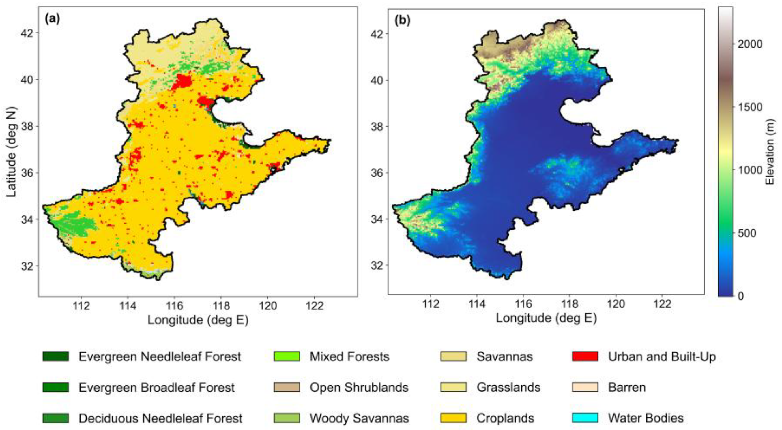
Figure 1. Land cover and elevation across the Huang–Huai–Hai Plain. Panel (a) shows land cover types derived from the Moderate-Resolution Imaging Spectroradiometer (MODIS) MCD12Q1 product [33], and (b) shows elevation derived from the Shuttle Radar Topography Mission (SRTM) digital elevation model.
Land 15 01701 g001
Figure 2. Environmental conditions across the Huang–Huai–Hai Plain during July 2023 and the 2018–2022 reference period. The figure presents the spatial distributions of Ta, SMrz, VPD, and DSR for (ad) July 2023, (eh) the 2018–2022 reference means for the same month, and (il) the corresponding July 2023 anomalies.
Land 15 01701 g002
Figure 3. July 2023 conditions assessed using historical percentiles across vegetated pixels in the Huang–Huai–Hai Plain: (a) Ta percentile, (b) SMrz percentile, (c) SPEI-1, and (d) co-occurrence of extreme heat and drought. Panels (a,b) map the historical percentiles of July 2023 Ta and SMrz relative to the 2001–2022 July distributions; panel (c) maps SPEI-1; and panel (d) identifies pixels where Ta exceeded P90 and SMrz fell below P10 simultaneously.
Land 15 01701 g003
Figure 4. SIF and GPP across the Huang–Huai–Hai Plain during July 2023 and the 2018–2022 reference period. Panels (ac) show the reference mean, July 2023 value, and anomaly for SIF, respectively; panels (df) show the corresponding GPP fields. GPP is expressed as the monthly mean daily rate derived from 8-day cumulative composites (g C m−2 d−1).
Land 15 01701 g004
Figure 5. Comparisons of SIF and GPP across vegetation types and elevation classes on the HHH Plain in July 2023. Panels (a,c) show vegetation classes and panels (b,d) show elevation classes. GPP is expressed as the monthly mean daily rate (g C m−2 d−1).
Land 15 01701 g005
Figure 6. Recovery trajectories of SIF anomalies from April to October 2023 across DBF, GRA, CRO, and elevation classes for pixels identified by the 2018–2022 standardized anomaly threshold (zi ≤ −1.5) together with a CRO phenology sensitivity comparison. Panel (a) shows monthly mean SIF anomalies for DBF, GRA, and CRO; panel (b) shows the trajectories for the 0–500 m, 500–1000 m, and >1000 m elevation classes; and panel (c) compares the proportions of CRO pixels with SIF anomalies ≥0 among affected CRO pixels and among the affected CRO subset identified as being in the active growing season.
Land 15 01701 g006
Figure 7. Spatial distribution of recovery timing and recovery proportions under the 2018–2022 standardized anomaly threshold (zi ≤ −1.5) across vegetation types and elevation classes on the Huang–Huai–Hai Plain. Panel (a) maps the first month in which SIF in affected pixels reached or exceeded its 2018–2022 monthly mean; panels (b,c) show the proportions of recovery classes across vegetation types and elevation classes, respectively. The mutually exclusive categories are ‘Not classified as affected’, ‘First recovered in August/September/October’, and ‘Not recovered by October’. Stacked bars use all pixels in each vegetation or elevation class as the denominator; recovery percentages in the text use affected pixels in that class.
Land 15 01701 g007
Figure 8. XGBoost–SHAP analysis of spatial associations between environmental anomalies and July 2023 SIF anomalies across DBF, GRA, and CRO with spatial cross-validation performance. Panel (a) reports mean absolute SHAP importance for DBF, GRA, and CRO, with the corresponding cross-validation R2 values based on 1° spatial blocks shown above the panel; panels (be) show SHAP response relationships for Ta, SMrz, VPD, and DSR anomalies, respectively. Faint points are pixel-level records and solid lines summarize responses within bins defined by predictor quantiles.
Land 15 01701 g008
Figure 9. XGBoost–SHAP analysis of SIF anomalies during recovery for pixels affected under the 2018–2022 standardized anomaly criterion (zi ≤ −1.5). Panel (a) shows grouped out-of-fold SHAP importance for recovery stage, initial July SIF loss, current DSR and its mean since July, current Ta and VPD and their means since July, current SMrz and its mean since July, and vegetation class; panels (be) show grouped SHAP responses for the initial July SIF anomaly, mean SMrz anomaly since July, mean VPD anomaly since July, and mean DSR anomaly since July, respectively. The header reports overall and vegetation-specific R2 from cross-validation using 1° spatial blocks for the recovery model.
Land 15 01701 g009
Table 1. Details of datasets used in this study, including variables, original spatial and temporal resolutions, study periods, and references. All SMrz analyses used GLEAM4.2a. The 2001–2023 daily record was aggregated to July monthly means for the long-term sensitivity and diagnostics of climatic extremeness.
Dataset/ProductVariableOriginal Spatial ResolutionOriginal Temporal ResolutionStudy PeriodReference
Global OCO-2 SIF (GOSIF)Solar-induced chlorophyll fluorescence0.05°8-day and monthly2018–2023; 2001–2022 long-term sensitivity[13]
MODIS GPP (MOD17A2HGF v6.1)Gross primary productivity500 m8-day2018–2023[34]
ERA5-Land2 m air temperature (Ta)~9 kmMonthly2018–2023; 2001–2022 extreme event diagnostic[36]
GLEAM4.2aRoot zone soil moisture (SMrz)0.1°Daily and monthly2018–2023 main; 2001–2023 sensitivity/diagnostic[37]
TerraClimateVapor pressure deficit (VPD)~1/24°Monthly2018–2023; 2001–2022 sensitivity[38]
TerraClimateDownward shortwave radiation (DSR)~1/24°Monthly2018–2023; 2001–2022 sensitivity[38]
ERA5–DroughtSPEI-10.25°Monthly2018–2023; 2001–2022 diagnostic[39]
MODIS phenology (MCD12Q2 v6.1)Phenology metrics500 mAnnual2018–2023[41]
SRTM DEM (SRTMGL1 v3)Elevation1 arc second (~30 m)StaticStatic[42]
Disclaimer/Publisher’s Note: The statements, opinions and data contained in all publications are solely those of the individual author(s) and contributor(s) and not of MDPI and/or the editor(s). MDPI and/or the editor(s) disclaim responsibility for any injury to people or property resulting from any ideas, methods, instructions or products referred to in the content.