Article

Quantifying the Shifting Nature–Human Dynamics of Soil Erosion in the Typical Black Soil Region of Northeastern China During 1980–2020


Heilongjiang Province Institute of Meteorological Science, China Meteorological Administration, Harbin 150030, China
*
Author to whom correspondence should be addressed.
Land 2026, 15(9), 1616; https://doi.org/10.3390/land15091616
Submission received: 7 June 2026 / Revised: 26 August 2026 / Accepted: 28 August 2026 / Published: 1 September 2026
(This article belongs to the Section Land–Climate Interactions)

Abstract

A quantitative assessment of the characteristics and driving mechanisms of black soil erosion is essential to sustainable agricultural development. In this study, we analyzed the spatiotemporal dynamics of the soil erosion modulus (SEM) in the Typical Black Soil Region (TBSR) of Northeast China from 1980 to 2020. The SEM dataset we utilized was derived from a high-resolution dataset utilizing the Revised Universal Soil Loss Equation (RUSLE) model. The independent and interactive effects of nine driving factors, including geographic, climatic, and anthropogenic variables, were quantified. Our findings are as follows: (1) The annual average SEM exhibited a slight but non-significant increase (0.002 t·ha−1·a−1), with a notable fluctuation since 2000. (2) While most regions demonstrated persistence with stability, areas with non-significant slight degradation trends were identified in parts of the eastern Inner Mongolia, Songnen, and Sanjiang subregions. (3) Slope and altitude emerged as the dominant factors influencing SEM patterns, with their effects substantially enhanced through interactions with other variables. Temporally, from the 2000 baseline to the 2001–2010 and 2011–2020 periods, the explanatory power of GDP consistently increased, contributing to an overall rise in anthropogenic influence that surpassed climatic factors. This trend indicated that human activities had increasingly impacted SEM patterns relative to climatic effects. (4) High-risk zones were identified at slopes of 6~8° and elevations of 1230~1430 m (approximately 0.2% of the region). These zones often overlap with ecologically fragile grassland situated in areas characterized by low socio-economic development. These findings underscore the nonlinear coupling mechanisms connecting human activities, land use, and climate systems, providing a scientific basis for targeted erosion mitigation and sustainable farmland management.

1. Introduction

Soil erosion in China ranks among the most severe globally. The first national water resources census conducted in 2013 revealed that the area affected by soil and water loss was 2.9491 × 10⁶ km2, which constitutes 30.72% of the nation’s total area [1]. The Northeast Black Soil Region, one of the three largest black soil regions worldwide and a major source of grain commodities for China, is experiencing significant degradation despite the relatively short period it has been used for agricultural cultivation. Soil erosion has affected approximately 2.16 × 10⁵ km2 of the region [2,3], resulting in a marked reduction in surface organic matter [4,5,6], furthermore, the thickness of the cultivated layer has decreased from 60 to 70 cm in the 1950s to 20–30 cm by around 2010 [7], leading to continuous reductions in the fertility and physical, chemical, and ecological properties of the soil [8,9]. The erosion process is driven by a combination of natural factors, such as the freeze–thaw cycle and concentrated rainstorms [10,11], and human activities like sloping ridge agriculture and high-intensity mechanical tillage [12,13,14]. Interactions between these mechanisms result in productivity losses and ecological consequences, including diffuse pollution and reservoir silting [15,16]. The interplay of these forces positions the Typical Black Soil Region (TBSR) as a critical case for understanding human–environment interactions, yet quantitatively distinguishing between natural and anthropogenic drivers and detecting shifts in their relative dominance over time poses a significant challenge.
Erosion processes in black soil regions are influenced by distinctive geomorphological features. In the Northeast Black Soil Region, these include subsurface interflow, sloped erosion on cultivated hillslopes, and reduced sediment transport in fluvial systems [10]. In recent decades, researchers have enhanced our understanding of the spatial extent and temporal dynamics of these processes, as well as the influence of land use and topography [6,15,16,17,18,19]. The climatic drivers of soil erosion encompass rainfall [11,20], freeze–thaw cycles [21,22], and aeolian activity [23], while anthropogenic influences include alterations in land use, tillage practices, and conservation measures. Recent investigations have highlighted the interactive effects of natural and anthropogenic factors on gully development [24,25], soil organic matter dynamics [26], and cropland productivity [27]. However, conventional attribution methods that rely on correlating individual climatic or human factors [28,29] fall short of capturing the nonlinear and interactive nature of human–land–climate interactions. Although remote sensing has made it easier to evaluate land-use changes [12], the relative contributions and interactions of natural and anthropogenic drivers remain inadequately quantified due to the scarcity of long-term high-resolution datasets and the underutilization of integrated analytical frameworks.
Previous research has primarily focused on quantifying erosion rates and their spatiotemporal dynamics [11,20,27]. Although attribution analyses have examined individual environmental factors, several areas remain insufficiently explored, including quantitative differentiation between natural and anthropogenic influences, the mechanisms of their interaction, and the identification of actionable risk thresholds. The contributions of natural and anthropogenic drivers to long-term soil erosion dynamics, the timing and extent of anthropogenic influence over the past decades, and the environmental thresholds for high-risk erosion zones also remain unclear. Liu et al. [11] established a soil erosion modulus (SEM) dataset for the Typical Black Soil Region (TBSR), providing a high-resolution characterization of spatiotemporal SEM trends and their relationship with extreme precipitation. Nonetheless, previous studies have not quantified the relative contributions of multiple driving factors or distinguished between natural and anthropogenic influences.
To address these gaps, we aim to achieve three objectives in the present study: (i) quantifying the independent and interactive effects of natural and anthropogenic drivers on SEM dynamics; (ii) detecting potential turning points in the relative dominance of these drivers from 2000 to 2020; and (iii) identifying risk thresholds for key influencing factors to inform targeted soil conservation strategies.

2. Materials and Methods

2.1. Study Area

The Typical Black Soil Region (TBSR) in Northeast China spans approximately 33.3 × 10⁴ km2 (117.03° E–135.79° E, 43.11° N–50.72° N), accounting for about 23.0% of Northeast China’s total land area. It encompasses 138 county-level administrative regions in Heilongjiang, Jilin, and Liaoning Provinces as well as the eastern part of Inner Mongolia (Figure 1) [30]. The region is characterized by black soils classified as Mollisols in the USDA Soil Taxonomy [31], which can be further categorized into two principal suborders based on local moisture and temperature conditions: Udolls (humid environments) and Ustolls (semi-arid environments). The primary land uses are farming (60.18%) and grazing (27.33%). Longitudinally, the region is segmented into three black soil subregions from west to east: eastern Inner Mongolia (EIMs, 9.5 × 10⁴ km2), Songnen (SNs, 21.2 × 10⁴ km2), and Sanjiang (SJs, 2.6 × 10⁴ km2) [30]. Agricultural activities are primarily concentrated in the SNs and the SJs, while the EIMs are predominantly utilized for grassland. The region experiences a temperate monsoon climate. As a critical agricultural region, the TBSR has undergone soil degradation in recent decades. The thickness of its black soil layer has decreased; originally 60–70 cm in the 1950s, it is currently 20–30 cm. In addition, a pronounced reduction in soil organic matter has been noted [7]. This degradation is influenced by a combination of natural factors [11,20] and anthropogenic activities [32], highlighting the necessity of quantifying the driving forces and identifying high-risk erosion zones for targeted mitigation strategies.

2.2. Data Source

The Revised Universal Soil Loss Equation (RUSLE) is widely utilized in soil erosion prediction [33]. This model integrates five factors (rainfall erosivity, soil erodibility, topography, cover management, and support practice) to estimate long-term average annual soil loss, performing effectively across extensive areas where direct field measurements are challenging [34,35]. Liu et al. [11] employed this model to estimate the SEM of the TBSR in Northeast China from 1980 to 2020 by incorporating meteorological and soil property data and remote sensing imagery. The soil property data for the RUSLE model were obtained from the World Soil Database, developed by the Food and Agriculture Organization (FAO) and the International Institute for Applied Systems Analysis (IIASA) [36]. The resulting SEM dataset features a spatial resolution of 500 m and a temporal resolution of one year, encompassing the period from 1980 to 2020. The model was validated against independent estimates for the Songnen Plain and compared with field-validated RUSLE applications, confirming the reliability of its output. However, the main uncertainties included the spatial interpolation of precipitation data, the representativeness of soil property data, and the empirical nature of the RUSLE model. This study builds upon this foundation.
Meteorological data were obtained from the China National Meteorological Science Data Center, which provides daily meteorological observation datasets encompassing daily temperature (T), precipitation (R), and sunshine duration (SS) recorded at 142 observatory stations. Annual mean meteorological values were calculated for each year from 1980 to 2020. To facilitate pixel-level analysis, the meteorological data were interpolated into 1 km gridded fields using Inverse Distance Weighting (IDW).
Normalized Difference Vegetation Index (NDVI) data were sourced from the NASA LP DAAC (Land Processes Distributed Active Archive Center), utilizing the MODIS/Terra Vegetation Indices 16-Day L3 Global 250 m SIN Grid product (MOD13Q1). To reduce noise and better align the time series with vegetation growth patterns, these data underwent preprocessing using a Savitzky–Golay filter [37]. Average NDVI values for the growing season (May to September) were employed to represent annual vegetation productivity. Additionally, the NDVI data were resampled to a spatial resolution of 500 m to correspond with the SEM grid for subsequent analysis.
Gross domestic product (GDP), population density (POP) and land use and land cover change (LUCC) data were obtained from China’s Resource and Environmental Science Data Platform, possessing a spatial resolution of 1 km × 1 km and generated through spatial interpolation based on national aggregate GDP statistics [38,39]. The dataset incorporates spatial variables such as nighttime light intensity, land-use types, and residential density, which were selected for their established correlations with human economic activity and population distribution at the county and district levels.
The digital elevation model (DEM) utilized in this study is the FABDEM (Forest and Buildings Removed Copernicus DEM) V1-2 dataset, which corrects height biases introduced by buildings and trees [40]. This dataset was supplied by the University of Bristol. Slope data were extracted from the DEM using ArcGIS 10.2. Table 1 presents a detailed summary of the datasets, sources, and attributes.

2.3. Method

The analytical framework of this study focuses on the nature–human system within the TBSR and was developed in three steps: (1) characterizing the spatiotemporal dynamics of the SEM from 1980 to 2020 using trend analysis including the Theil–Sen Median trend and Mann–Kendall test, along with the Hurst exponent to assess persistence; (2) quantifying the independent and interactive effects of driving factors on SEM patterns through the geographical detector; and (3) distinguishing the relative contributions of climate change and human activities using residual trend analysis. The geographical detector analysis was performed for the period encompassing 2000 to 2020, while the residual trend analysis was conducted using meteorological data from 1980 to 2020.

2.3.1. Temporal Aggregation and Segmentation

Given that our overarching research period spans 1980 to 2020, period-based segmentation was implemented to optimally utilize available data while clearly delineating the temporal scope of various analyses. For GDP, POP, and LUCC, which were available only at discrete time points, the 2000 data reflect the socio-economic conditions at the outset of the analysis period. In contrast, the 2010 and 2020 data represent the mean states for the 2001–2010 and 2011–2020 periods, respectively. For the NDVI, period-averaged values were calculated for the same two decadal intervals. Analyses were conducted for the temporal trends and persistence of the SEM, along with residual trend analyses utilizing meteorological data, for the entire 40-year period.
Our geographical detector analysis was restricted to the period encompassing 2000 to 2020, owing to the lack of earlier continuous high-resolution gridded socio-economic data for GDP, POP, and LUCC. Notably, the 2000 data serve as a single-year snapshot, while the periods from 2001 to 2010 and from 2011 to 2020 are represented as decadal means. Therefore, the 2000 data were utilized as a descriptive baseline, while we used data from the periods spanning 2001 to 2010 and 2011 to 2020 to analyze changes caused by drivers.

2.3.2. Theil–Sen Median Trend

Theil–Sen Median trend analysis provides a non-parametric approach for estimating linear trends in non-normally distributed data, particularly in the presence of small outliers and missing values [41]. Since the SEM time series do not meet the assumptions of normal distribution, this method is suitable for identifying long-term trends in erosion data. The calculation method is as follows:
β = Median y j y i j i , f o r   i < j
where β is the median value of the slope between the yi and yj data corresponding to the years i and j, respectively. If β > 0, it indicates an upward trend in the SEM, reflecting intensified erosion and soil degradation. Conversely, if β < 0, it indicates a downward trend in the SEM, suggesting reduced erosion and soil improvement.

2.3.3. Mann–Kendall Test

The Mann–Kendall test is a non-parametric method suitable for data that does not follow a normal distribution, as the presence of missing or abnormal values does not compromise the precision of the test results [42]. This test was employed in combination with the Theil–Sen estimator to assess the statistical significance of the detected trends.
S = i = 1 n 1 j = i + 1 n sign y j y i
where yi and yj are sequential data values for a time series of length n, and
sign y j y i = 1 , y j y i > 0 0 , y j y i = 0 1 , y j y i < 0
Under the null hypothesis that the data are independent and identically distributed, the mean of S is zero, and the variance of S is
var S = 1 18 n n 1 2 n + 5 i = 0 m t i t i 1 2 t i + 5
where n is the number of observations in the time series, m is the number of tied groups in the time series (a tied group is a collection of sample data with the same value), and ti is the number of data points in the ith group. The Z statistics are calculated as follows:
Z = S 1 var S , S > 0 0 , S = 0 S + 1 var S , S < 0
The Z statistic lies within the range (−∞, +∞). A specific significance level, Z > u 1 α / 2 , denotes the extent to which the time series demonstrate significant trends at the level of α. In this study, α = 0.05, meaning that the trends were assessed at a confidence level of 0.05 for the period from 1980 to 2020.

2.3.4. Hurst Exponent

The Hurst exponent method can be used to determine the persistence of time series data [43,44] and has been extensively applied to detect variations in time series [45,46]. In this study, the R/S analysis method was applied to calculate the Hurst exponent. Given a time series ξ(t), i = 1, 2, …, n, for any positive integer τ, the mean sequence is defined as follows.
ξ t ¯ = 1 τ t = 1 τ ξ t , τ = 1 , 2 , , n
Cumulative deviation:
X t , τ = τ = 1 t ξ t ξ τ ¯ , 1 t τ
Range sequence:
R τ = max 1 t τ X t , τ min 1 t τ X t , τ , τ = 1 , 2 , , n
Standard deviation:
S τ = 1 τ t = 1 τ ξ t ξ t ¯ 2 1 / 2 , τ = 1 , 2 , , n
If the relationship R / S τ H holds for the rescaled range, it indicates the presence of the Hurst phenomenon in the analyzed time series. H, the Hurst exponent, ranges from 0 to 1 and can be obtained using least squares (ln τ, ln R/S) within a double logarithmic coordinate system. When H < 0.5, the SEM time series exhibits an anti-persistence, indicating that the current trend is likely to reverse in the future; when H ≈ 0.5, the time series is characterized as random and non-persistent, suggesting that future trends are independent of past trends; and when H > 0.5, the time series demonstrates persistence, implying that future trends will align with those observed during the study period. These classifications provide our basis for assessing the persistence of SEM trends.

2.3.5. Geographical Detector

The geographical detector model is a spatial analysis tool designed to identify the driving factors underlying specific geographical and economic phenomena [47]. Additionally, it facilitates the exploration of relationships between detection elements and measures of spatial heterogeneity. It consists of four parts: a factor detector, an interactive detector, an ecological detector, and a risk detector. This model was employed to investigate the influence of the nine factors listed, as outlined in Table 1, on the SEM. The factor detector is defined as follows:
q = 1 1 n σ 2 h = 1 L n h σ h 2
where the number of layers h of the independent variable ranges from 1 to L, and L is the total number of layers used for the discretization of continuous variables. The units and variance of layer h are denoted by nh and σh2, respectively. The units and variance of the study area are represented by n and σ2, respectively. q signifies the explanatory power of the independent variable on the dependent variable, with values ranging from 0 to 1. A q value closer to 1 indicates that the factor has stronger explanatory power. Consequently, the dominant factors influencing the SEM can be identified through a comparison of q values. The significance of q can be assessed using the geographical detector model. However, q values do not provide standard errors or confidence intervals, as they rely on variance comparison rather than parametric inference. The primary advantage of the geographical detector over other statistical methods is its ability to detect interactions. The interaction detector compares q values of single factors and paired factors to ascertain the type and direction of interaction between two factors; the ecological detector evaluates whether two factors provide significantly different explanations for the geographical distribution of the dependent variable; and the risk detector identifies areas with high risk of soil erosion associated with specific factor ranges and evaluates whether the dependent variable exhibits significant differences across stratified layers.
The geographical detector requires that input variables be discrete. LUCC, being inherently categorical, is directly applicable. For continuous variables, we employed various statistical discretization techniques, including equal intervals, natural breakpoint, quantiles, geometric spacing, and standard deviation, to determine the most suitable categorization scheme. Elevation was classified into ten categories using the equal interval method; slope, T, and R were stratified into ten categories with the natural breakpoint, equal interval, and geometric interval methods; SS and NDVI were classified into eleven categories using the natural breakpoint. GDP was segmented into twelve categories using the quantile approach, and POP was discretized into ten classes using geometric intervals. The resulting raster layers were transformed into point features through ArcGIS 10.2’s Fishnet function on a 1 km grid, which served as the input for the geographic detector analysis.

2.3.6. Residual Trend Analysis

A residual trend analysis was employed to differentiate the impacts of climatic and non-climatic factors on the SEM. This analysis was predicated on the hypothesis that the non-climatic component of the SEM can be isolated after accounting for the effects of climatic factors [29,48]. Specifically, a multiple regression model was developed with temperature, precipitation, and sunshine duration as independent variables and the SEM as the dependent variable. The predicted values derived from this regression represent the climate-induced baseline of the SEM, while the residuals, defined as the difference between the actual and predicted SEM values, are ascribed to the non-climatic component.
SEM C C = a × R + b × T + c × S S + d
SEM N C = SEM SEM C C
K = n × i = 1 n i × y i i = 1 n i i = 1 n y i n × i = 1 n i 2 i = 1 n i 2
where R, T and SS are the mean precipitation, temperature, and sunshine duration, respectively, with the parameters a, b, c, and d introduced as model coefficients. The predictive SEM value derived from the multiple regression equation is represented by SEMCC, which reflects the climate-driven component determined by temperature, precipitation, and sunshine duration. The residuals, defined as the difference between actual and predicted SEMCC, are denoted as SEMNC, representing the non-climatic component. The slope K indicates the rate of temporal change. The number of years is represented by n, while i is the time variable. The variable yi represents the SEM value influenced by either the climate-driven or non-climatic component. The residual analysis was performed at the pixel level using annual SEM and meteorological data from 1980 to 2020. This methodology enables the non-climatic component of SEM variation to be isolated. Table 2 shows six classifications derived from the residual trend analysis. Unlike the geographical detector, which examines pairwise interactions between factors, the residual trend analysis distinguishes between climatic and non-climatic influences on the SEM and indicates, through the slope K, whether their contributions are positive or negative.

3. Results

3.1. The Temporal Variation Characteristics of the SEM

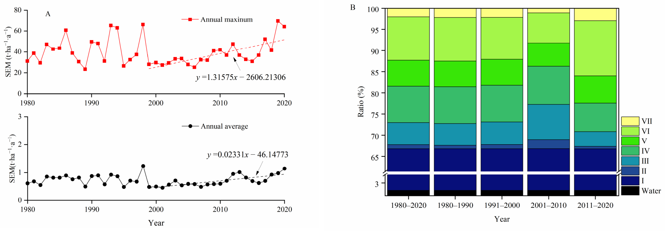
Figure 2A displays the temporal dynamics of the TBSR’s SEM from 1980 to 2020. The annual average SEM exhibited considerable variability, ranging from 0.46 t·ha−1·a−1 in 2001 to 1.24 t·ha−1·a−1 in 1998, with overall trends indicating a slight but non-significant increase of 0.002 t·ha−1·a−1 (p > 0.05). Annual maximum SEM values showed greater fluctuations, ranging from 23.41 t·ha−1·a−1 in 1998 to 69.60 t·ha−1·a−1 in 2019, though the trend (0.093 t·ha−1·a−1) was also not statistically significant (p > 0.05). After 1999, both values displayed significant upward trends (p < 0.05), with rates of 0.023 t·ha−1·a−1 and 1.349 t·ha−1·a−1, respectively.
A classification system was previously developed based on the Chinese “Soil Erosion Classification and Grading Standards” (SL 190–2007) [49]. In the study area, this standard designates slight erosion as <2 t·ha−1·a−1, light erosion as 2~25 t·ha−1·a−1, and moderate erosion as 25~50 t·ha−1·a−1. Given that the SEM primarily falls within the slight and light erosion categories in the TBSR, with moderate and higher grades comprising a negligible proportion (<0.01%) of the total area, we refined the classification into seven grades to more accurately reflect the spatial heterogeneity within the predominant erosion classes: Grade I: ≤0.2 t·ha−1·a−1; Grade II: 0.2–0.5 t·ha−1·a−1; Grade III: 0.5–1.0 t·ha−1·a−1; Grade IV: 1.0–1.5 t·ha−1·a−1; Grade V: 1.5–2.0 t·ha−1·a−1; Grade VI: 2.0–5.0 t·ha−1·a−1; Grade VII: >5.0 t·ha−1·a−1.
Figure 2B shows the proportional changes in these grades across different decades. Grade I exhibited stability throughout the study period. Compared to the distribution from 1991 to 2000, Grades II, III, and IV increased by 1.2%, 2.9%, and 0.4%, respectively, during 2001–2010, while Grades V–VII decreased by 4.5%. In contrast, during the 2011–2020 period, a reversal was observed; Grades II–IV decreased while Grades V–VII expanded. Notably, Grade VI increased by 6.0%, reaching 13.1%. In summary, the SEM remained stable from 1980 to 2000, followed by an increase in the lower grades (II–IV) and a decrease in the higher grades (V–VII) during the 2001–2010 period, with an inverse trend observed during 2011–2020.

3.2. The Spatial Characteristics of the SEM

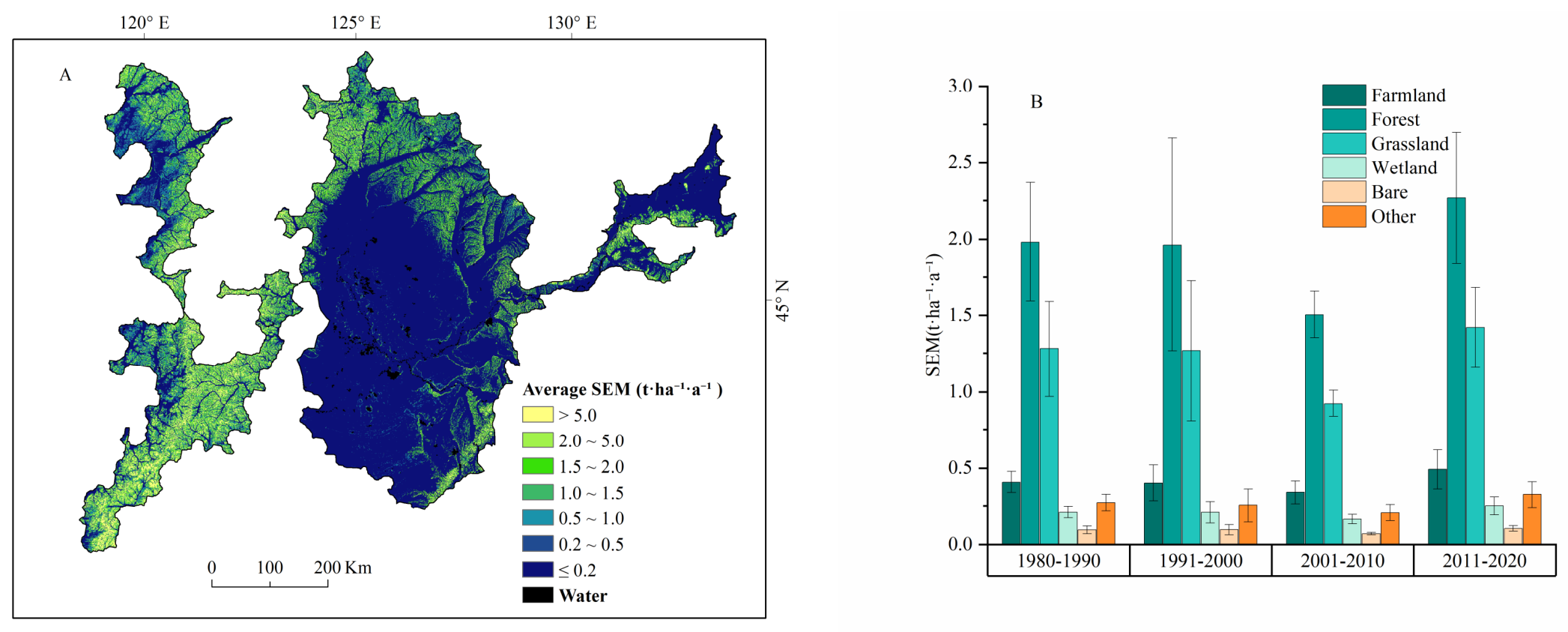
Based on the seven-grade classification outlined above, Figure 3A shows the spatial heterogeneity of the TBSR’s SEM from 1980 to 2020. The average SEM was 0.71 t·ha−1·a−1, with a range spanning from 0 to 34.12 t·ha−1·a−1. The SEM in the SNs and SJs was lower than that observed in the EIMs. From 1980 to 2020, the average SEM predominantly fell within Grade I (65.5%) and Grade VI (10.2%), accounting for 75.7% of the study area when combined. The remaining Grades (II, III, IV, V, and VII) exhibited gradients of spatial distributions, with proportions varying from 1.0% to 8.5%, where Grade IV exhibited the highest proportion at 8.5%.
Figure 3B presents the spatial distribution of average SEM across various land-use types by decade, from highest to lowest: forest, grassland, farmland, other land, wetland, and bare land. Interdecadal fluctuations exhibited stability from 1980 to 2000, transitioned to a marked decline from 2001 to 2010, and culminated in a resurgence from 2011 to 2020.

3.3. The Variation in Trends of SEM

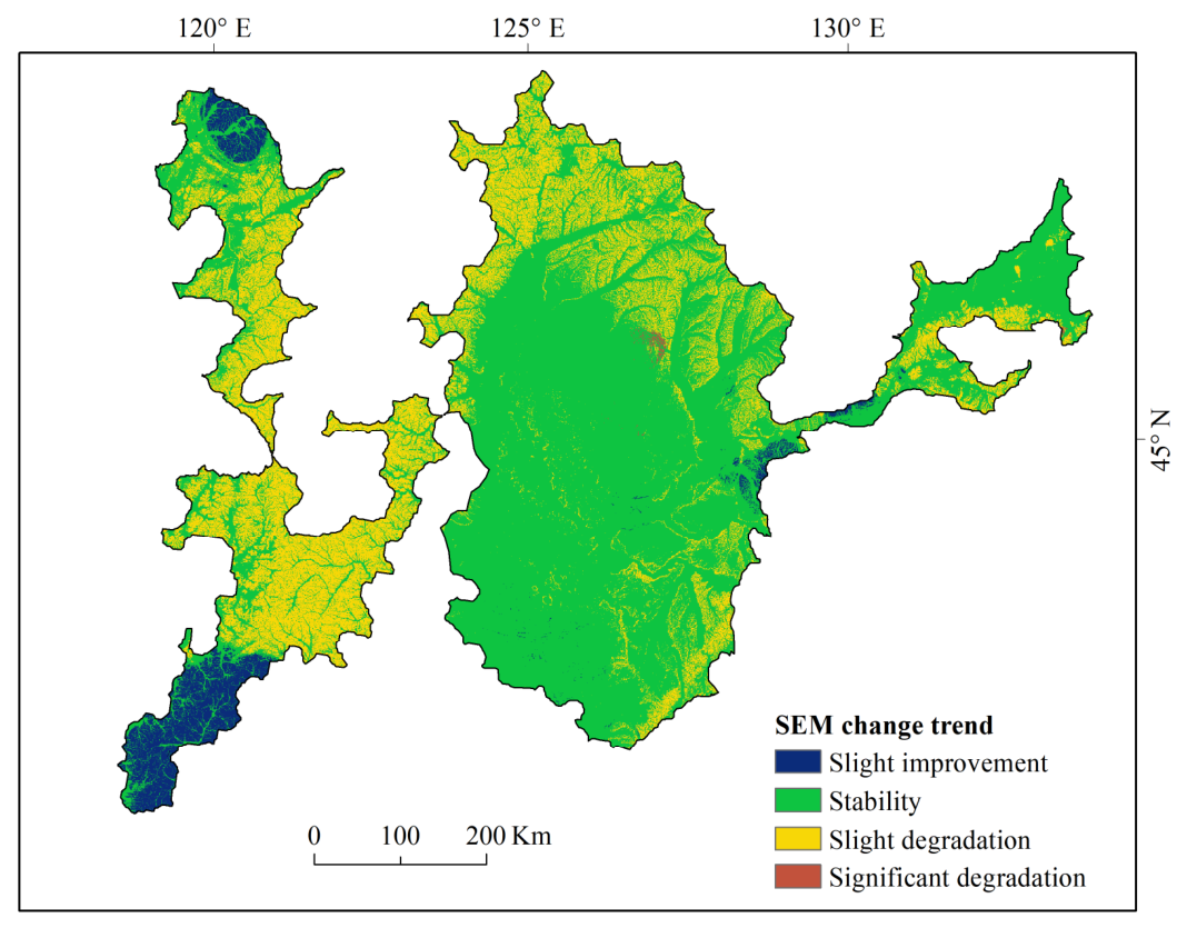
The Theil–Sen Median trend analysis and the Mann–Kendall test were applied to identify the temporal variations of individual pixels and to elucidate the spatial distribution of SEM trend fluctuations across the TBSR. As regions with an exact β of 0 were absent, classification was based on the actual β values: areas with β values between −0.0005 and 0.0005 were classified as stable, those with β ≥ 0.0005 as degraded, and those with β < −0.0005 as improved. The Mann–Kendall test (p < 0.05) was employed to evaluate trend significance, with |Z| > 1.96 indicating significant change and |Z| ≤ 1.96 indicating insignificant change. Table 3 presents the four classification schemes derived from the combined results of the Theil–Sen Median and the Mann–Kendall test. Figure 4 shows the spatial distribution of SEM trends across the TBSR. At the regional scale, areas that demonstrated slight degradation, stability, and slight improvement accounted for 26.8%, 67.2%, and 4.6% of the total area, respectively, while significant degradation accounted for only 0.1%. At the subregional scale, the northern and southern parts of the EIMs exhibited slight improvement; the majority of the SJs and the central–southern parts of the SNs displayed stable SEM; slight degradation was observed in the central EIMs, northern and southeastern SNs, and localized areas of the SJs; and significant degradation was detected in the northern parts of the SNs.
To assess the persistence of the SEM trends, the Hurst exponent was combined with Theil–Sen Median trend analysis and the Mann–Kendall test. In this context, persistence refers to the probability that an identified trend will extend into the future, as indicated by the Hurst exponent. Table 4 displays seven combinations of trend and persistence types, of which the last four were associated with non-persistence, indicating that future trends could not be reliably predicted.
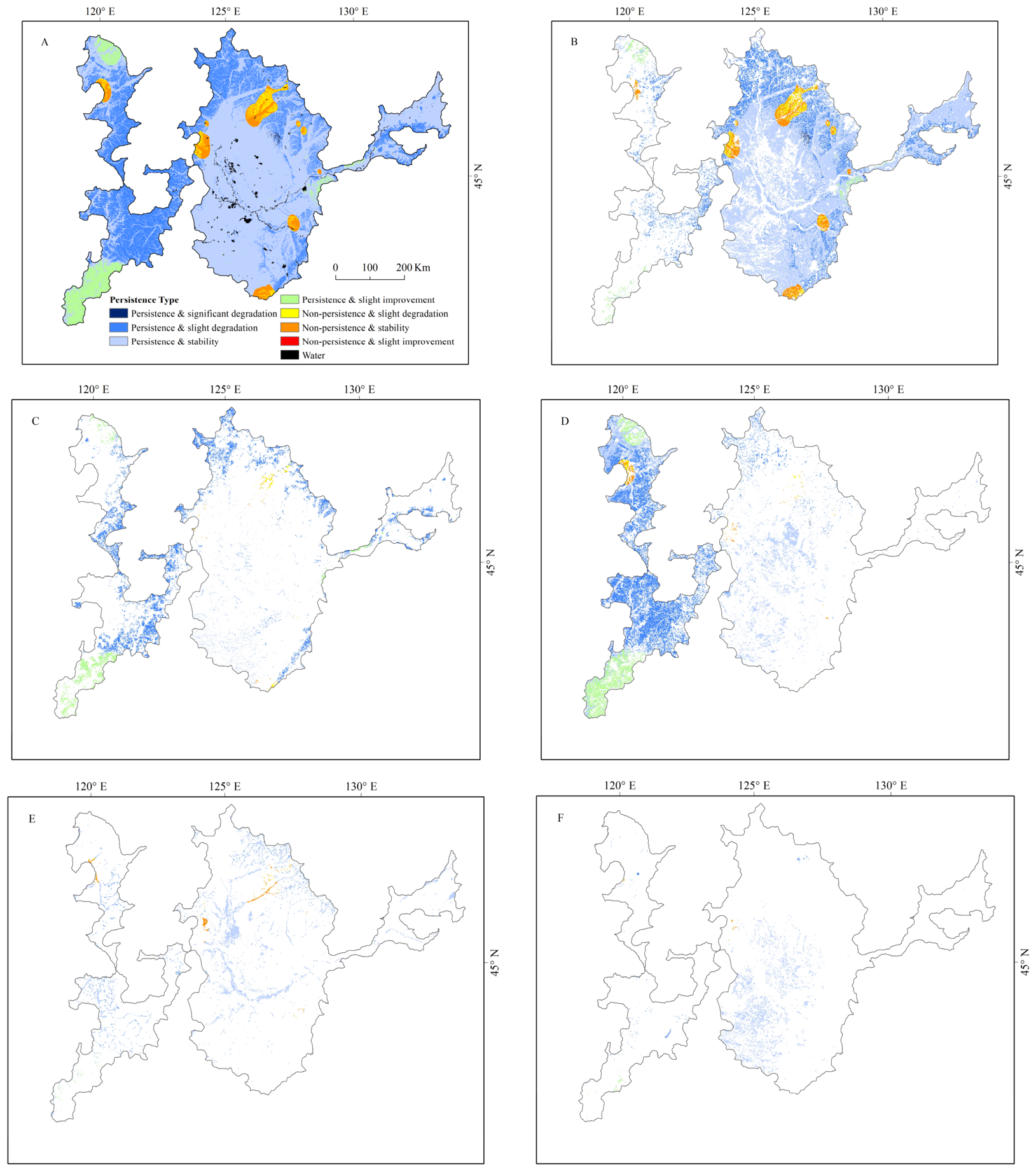
Figure 5 and Table 4 illustrate the spatial distribution of persistence patterns: 4.6% of the area exhibited persistence with slight improvement, predominantly located in the northern and southern parts of the EIMs; the majority of the regional area (64.1%) demonstrated persistence with stability, primarily situated in the central–southern SNs and the majority of the SJs; 25.6% of the total area exhibited persistence with slight degradation, mainly concentrated in the central EIMs, the northern and southeastern SNs, and localized areas of the SJs; and 0.1% of the total areas demonstrated persistence with significant degradation, identified in the northern SNs. Finally, the yellow and red areas in Figure 5A, representing 4.4% of the total area, exhibited non-persistent trends, primarily in the northwestern EIMs and northern and southern SNs, and require further assessment.
Figure 5B–F illustrates the stability of various land use types, exhibiting significant spatial heterogeneity. The trends and persistence analysis indicate that grassland (2.6%), forest (1.3%), and farmland (0.7%) showed persistence with slight improvements. In contrast, farmland (39.4%), grassland (11.3%), and wetland (5.0%) maintained persistence with stability. Additionally, farmland (10.2%), grassland (9.2%), and forest (6.3%) exhibited persistence with slight degradation. Proportionally, farmland, grassland, and wetland were the primary stable geomorphological components within the TBSR with respect to the SEM, with farmland and grassland displaying particularly high stability.

3.4. Driving Mechanisms

To explore the multifactorial mechanisms driving SEM trends, interannual variations were analyzed. Utilizing 2000 as a descriptive baseline, the study period was segmented into three intervals: 2000, 2001–2010, and 2011–2020, with the latter two consistent with the division outlined in Section 3.1. A geographical detector model, including factor, interaction, and risk detectors, was employed to quantify the influence of various determinants on the SEM within each interval.
Table 5 summarizes the environmental determinants and their corresponding q values. In 2000, the primary environmental drivers were ranked as follows: slope > altitude > POP > T > SS > GDP. From 2001 to 2010, the ranking changed to slope > altitude > T > GDP > POP > SS, and from 2011 to 2020, a further change was seen: slope > altitude > GDP > POP > T > SS. Slope and altitude exerted significantly stronger influences on the SEM than other factors, both showing a “V-shaped” pattern: an initial decline followed by an increase. In 2011–2020, their q values reached 0.396 and 0.298, respectively, indicating their strong explanatory power in shaping the SEM patterns in the TBSR. GDP exhibited a notable and consistent trend, with its q value rising from 0.041 in 2000 to 0.080 during 2001–2010, and further increasing to 0.137 in 2011–2020. In contrast, POP showed a non-monotonic pattern (0.111, 0.075, and 0.099), while T and SS remained relatively stable.
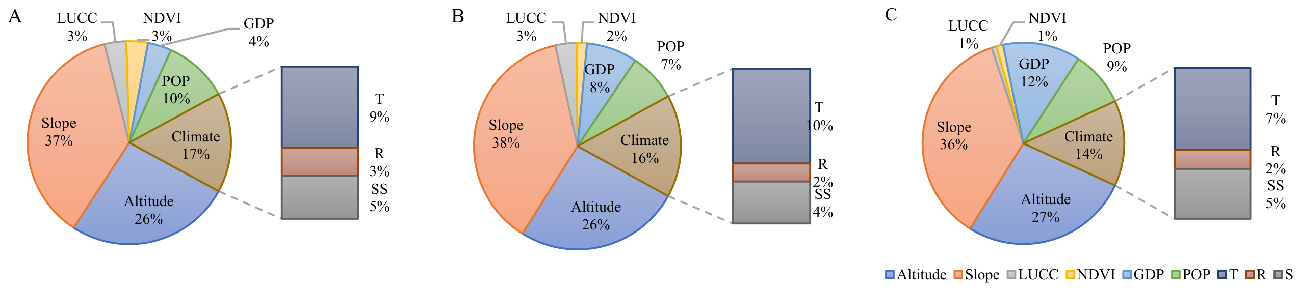
Figure 6 shows the rescaling of individual q values for each environmental factor across the three analytical periods. In 2000, the combined rescaled contributions of slope, altitude, and climatic factors (T, R, and SS) exceeded 70%, with climatic factors accounting for 17% and anthropogenic factors (GDP and POP) accounting for 14% of the total q value. From 2001 to 2010, the rescaled contribution of climatic factors slightly decreased to 16%, while the contribution of anthropogenic factors increased marginally to 15%. From 2011 to 2020, a more pronounced shift occurred, as the rescaled contribution of anthropogenic factors rose to 21%, surpassing that of climatic factors, which declined to 14%. Within the anthropogenic category, GDP emerged as the primary driver of this increase, with its relative contribution rising from 4% in 2000 to 12% in 2011–2020, whereas POP did not exhibit a consistent trend.
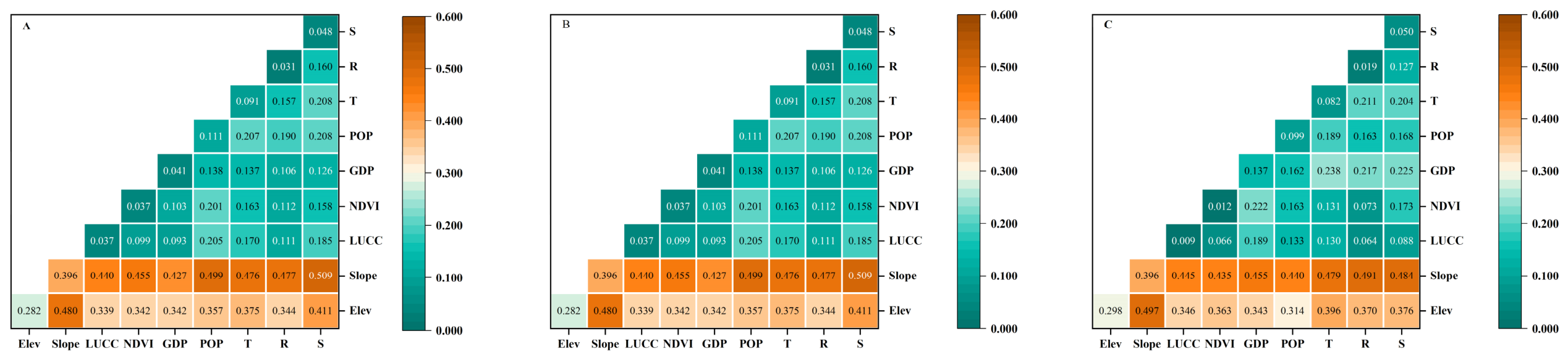
As shown in Figure 7, the interaction detector indicated that all pairwise interactions among environmental variables enhanced the explanatory power of the SEM. The dominant types of interactions varied over time. In 2000 and the 2001 –2010 period, the top five interactions by explanatory strength were slope ∩ SS, slope ∩ POP, slope ∩ altitude, slope ∩ R, and slope ∩ T. From 2011 to 2020, this order shifted to slope ∩ altitude, slope ∩ R, slope ∩ SS, slope ∩ T, and slope ∩ GDP. The interaction between slope and SS was a significant explanatory factor for the SEM in both 2000 and the 2001–2010 period, consistently exceeding 50.0% in explanatory power. This suggests that spatial variations in solar radiation or differences in SS across slopes influence SEM variability. In the 2011–2020 period, the interaction between slope and altitude emerged as the most explanatory (49.7%), while the influence of slope and SS slightly declined to 48.4%. Overall, the second- to fifth-highest interactions all involved slope interactions with a single environmental factor, although the specific factors changed over time. Furthermore, these interactions enhanced the explanatory power of individual factors, exhibiting nonlinear or bivariate enhancement.
Table 6 presents the threshold ranges (high-risk zones) for each factor, as identified by the risk detector at a 95% confidence level. The sensitivity of these zones exhibited variation across different periods. For topographic factors, specifically altitude and slope, the high-risk zones remained consistent, with altitudes ranging from 1230 to 1430 m and slope ranging from 6° to 8° across all periods. This combined area accounted for approximately 0.19% of the total TBSR area, predominantly located within the EIMs. The LUCC analysis indicated that grassland was primarily located within high-risk zones in 2000 and 2011–2020, while wetland was primarily located within high-risk zones in the 2001–2010 period. For the NDVI, the high-risk zones consistently fell within the 0.63~0.85 range across all periods. Furthermore, these high-risk zones were consistently associated with low GDP and POP across all periods. Climatic conditions associated with high-risk zones generally included lower temperature, less precipitation, and longer sunshine duration.
The LUCC strata identified as high-risk by the risk detector (grassland in 2000 and 2011–2020, wetland in 2001–2010) differ from the land-use hierarchy shown in Figure 3B, in which forest exhibits the highest mean SEM. These results are not directly comparable. The risk detector evaluates each factor independently; for a categorical variable such as LUCC, the strata are the land-use classes themselves, and the comparison is made across the mean SEM of those classes at the 1 km Fishnet sampling points, aggregated over the period-specific intervals defined in Section 2.3.1. Figure 3B, by contrast, reports decadal mean SEM computed over all 500 m pixels within each land-use class. Differences in sampling support and in temporal aggregation are sufficient to account for the divergent rankings, and neither result reflects the topographic or socio-economic ranges reported in Table 6.

3.5. Relative Contribution of Climate Change and Non-Climatic Factors to SEM

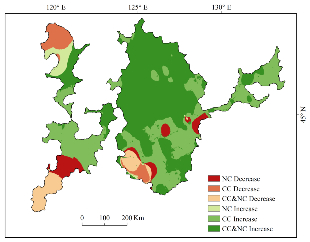
As shown in Figure 8, the climate-driven (CC) and the non-climatic components (NC) were the primary drivers of SEM spatial patterns. Approximately 47.6% of the study area experienced increases in SEM where both CC and NC were positive, indicating that these two driving forces acted in concert rather than counteracting one another. The locations where SEM increases were attributed to CC comprised about 32.8% of the total area, predominantly located in the central EIMs, southern SNs, and most of the SJs. Increases due solely to NC occurred in 2.8% of the total area, primarily in the northern EIMs. Areas exhibiting SEM decreases due to combined influences accounted for roughly 5.4% of the total area, mainly in the southern EIMs and southwestern SNs. Areas where SEM decreases were exclusively associated with CC or NC accounted for 4.9% and 5.0% of the total, respectively, primarily across the northern and southern EIMs and localized parts of the central and southwestern SNs. The remaining 1.5% of the study area, including water bodies and no-data pixels, displayed no discernible trend and was therefore not classified into any of the six categories. Overall, the combined effects of CC and NC emerged as the primary factors influencing SEM variation over the study period, indicating an intensification in black soil erosion.

4. Discussion

4.1. The Severity of the SEM Within the TBSR

Soil erosion is widely acknowledged as a major environmental threat to terrestrial ecosystems, adversely affecting habitats and agricultural productivity [50]. Between 2001 and 2012, approximately 38% of agricultural land experienced degradation due to erosion, while global soil erosion increased by 20% [51]. Although the severity of this issue is less pronounced than in southern China, soil and water loss in Northeast China remains a considerable concern [9,18,52]. The mean SEM in the TBSR, at 0.71 t·ha−1·a−1, is relatively low compared to the global average of approximately 2.8 t·ha−1·a−1 reported by Borrelli et al. [51] for 2012. Studies in other major black soil regions, such as the US Corn Belt and the Ukrainian Chernozem region, have indicated soil erosion rates that are generally higher than those observed in the TBSR under conventional tillage practices [53,54]. However, differences in RUSLE parameterization, including spatial resolution, methods for calculating rainfall erosivity, and formulation of the C factor, should be considered when interpreting these discrepancies. The distribution of erosion exhibits extensive heterogeneity across various land-use types and geomorphological features. Effective erosion control in the TBSR is essential for ensuring food security and promoting sustainable socio-economic development at both regional and national levels [55]. Therefore, investigating the spatial characteristics of soil erosion and the mechanisms driving it is of great significance for prioritizing areas for prevention and control, as well as for optimizing mitigation strategies.

4.2. Spatial and Temporal Patterns of SEM

Based on the SEM dataset provided by Liu et al. [11], our study revealed further insights into the spatiotemporal dynamics in the TBSR. The annual average SEM showed a slight, non-significant increase from 1980 to 2020, with fluctuating growth since 2000. The spatial distribution exhibited significant heterogeneity, with lower SEM in the SNs and SJs compared to the EIMs. Although most areas demonstrated stability, localized areas of degradation were identified across all three subregions.
Although the linear trend over the entire period from 1980 to 2020 was not statistically significant, distinct stage characteristics were present from 2000 onwards, particularly after 2010, when the SEM began to exhibit upward fluctuations, indicating increasing erosion pressure. This recent intensification is consistent with the findings of Liu et al. [11] and Yang et al. [52], who associated erosion with the frequency and intensity of extreme precipitation in the region. In terms of spatial patterns, areas characterized by persistence with stability constituted the largest proportion, followed by areas exhibiting persistence with slight degradation. Further analysis identified that farmland, grassland, and forest represent the three primary land use types contributing to the SEM. The impact of land- use configuration and structural composition on erosion rates varied significantly. The TBSR, a primary grain production zone in China, predominantly employs a single cropping system on a one-year cycle. Traditional farming practices prevail, leading to extended periods of soil exposure. As cultivation years increase, soil erosion intensifies, leading to downward movement of mineral-associated organic carbon [56,57].

4.3. Driving Mechanism Transformation and Factor Interaction

The process of the SEM’s environmental response is complex and influenced by various geo-environmental factors [6]. The analysis showed that topographic factors, especially slope and altitude, played a major role in shaping SEM spatial distribution. Temporally, as we moved from the 2000 baseline to the two subsequent decadal periods (2001–2010 and 2011–2020), the explanatory power of climatic factors declined, while anthropogenic factors, including GDP and POP, exhibited a consistent increase. Consequently, a shift emerged in 2011–2020, when the combined influence of anthropogenic factors surpassed that of climatic factors. It is important to note that within the anthropogenic category, this aggregate increase is primarily attributable to GDP, as POP did not exhibit a consistent trend. This decadal-scale transition indicates the growing significance of human activities relative to climatic influences on SEM patterns.
Our analysis indicated that the interactions between slopes and various factors, such as precipitation, temperature, and human activities, exceeded their individual effects. Sloping farmland under traditional vertical ridge farming systems continues to be the main source of erosion and deposition, further supporting the necessity of restricting cultivation on steep slopes [17]. Furthermore, the interaction between slopes and climatic factors greatly enhanced their explanatory power for erosion risk. The widespread prevalence of strong interaction effects highlights the inherent complexity and vulnerability of the erosion system [58].
The risk detector analysis identified that high-risk zones overlapped areas characterized by lower POP and relatively low GDP. This finding challenges the view that severe erosion is predominantly associated with densely populated and economically developed areas [48]. Notably, areas with elevations of 1230~1430 m and slopes of 6~8° showed the highest erosion sensitivity and were primarily located within the EIMs, accounting for approximately 0.19% of the total TBSR area. Although the EIMs mainly comprise grassland, they also encompass sloping farmland, rendering these areas particularly vulnerable to erosion under conventional tillage practices. Field studies have identified that a slope of 6° serves as a critical threshold for erosion processes in the Mollisol region [19], beyond which the RUSLE slope factor increases nonlinearly [33]. Additionally, a slope of 8° corresponds to the transition from slight to moderate erosion according to the Chinese standard SL 190–2007 [49]. This elevation range coincides with a topographic transition zone, where steeper gradients facilitate concentrated runoff [59]. From a practical perspective, these high-risk zones correspond to various land use contexts including grassland, sloping farmland, and wetland, each requiring differentiated management approaches that consider local conditions. As climate change intensifies, these areas become increasingly susceptible to erosion, while economically developed regions show greater resilience due to investments in soil conservation and enhanced vegetative cover. Multiple mechanisms contribute to these spatial patterns. Clay-rich subsoil and cultivation-induced plow pans facilitate aggregate breakdown and interflow, thereby increasing erodibility [19]. Extreme rainfall events (≥25 mm/day) demonstrate the strongest correlation with soil erosion, as raindrop impact can exacerbate soil loss [11]. Vegetation cover mitigates erosion through canopy interception and root reinforcement, while post-harvest bareness leaves the soil vulnerable to both water and wind erosion [59]. Conservation tillage effectively reduces erosion, with contour ridge tillage proving beneficial on slopes of less than 10°, while downslope-oriented ridges on sloping farmland can accelerate runoff [17]. Wind erosion, particularly significant in the western subregion during spring, interacts with water erosion to amplify overall soil loss [23]. These interaction effects (Table 5; Figure 7) underscore that erosion processes in the TBSR are governed by complex, nonlinear relationships between terrain, climate, and anthropogenic factors, indicating that single-factor attribution is inadequate for fully explaining the observed patterns.

4.4. Research Limitations and Prospects

In summary, this study, building upon the high-resolution dataset of Liu et al. [11], enhances our understanding of the SEM’s spatiotemporal evolution within the TBSR. It identifies a decadal-scale shift in the influencing forces and underscores the role of topographic factors as interpreted within the RUSLE framework.
Several limitations should be acknowledged when interpreting the attribution results. First, a methodological caveat pertains to the relationship between the driving factors and the construction of the SEM dataset. The SEM was generated using the RUSLE model, in which slope and altitude are incorporated through the LS factor, precipitation through the R factor, and NDVI and LUCC through the C factor. Given that the K, LS, and P factors in the RUSLE model remain stable over time, interannual variation in SEM is primarily influenced by changes in R and C factors. After the climatic signal is removed through regression, the residual is predominantly determined by the time-varying C factor (NDVI and LUCC), signifying that the non-climatic component reflects changes in vegetation and land cover rather than serving as a direct indicator of human activity. Nevertheless, GDP and POP provide the most compelling evidence of genuinely independent anthropogenic influence. Thus, this methodological qualification does not undermine the evidence for increasing human impact. Second, the resolution of the SEM dataset constrains its capacity to capture gully-scale features. However, as demonstrated in our previous study [11], the erosion rates are consistent with independent estimates and field-validated applications. The primary objective is regional-scale attribution, for which the dataset provides a consistent foundation. The identified trends and shifts in drivers depend on the consistency of the dataset rather than its absolute resolution. Third, due to the lack of high-resolution spatial data during the early study period, socio-economic factors (GDP, POP) for 1980–2000 are represented by the data from the year 2000. This assumption inevitably introduces uncertainty. Fourth, the residual trend method may inadequately account for time-invariant geographical factors; their exclusion from the regression implies that topographically induced variation not captured by climatic covariates is absorbed into the residual term. This could lead to an overestimation of the non-climatic component, particularly in topographically heterogeneous regions such as the EIMs. Since topographic effects were time-invariant, this bias does not undermine the observed increasing trend of the non-climatic component after 2011, although its absolute magnitude may be overestimated. The NDVI thresholds identified by the risk detector were not analyzed separately for various land use types, and the spatial descriptions of degradation patterns should be interpreted with the methodological limitations discussed above in mind. Furthermore, the pixel-wise Mann–Kendall trend tests were neither corrected for multiple comparisons nor adjusted for serial autocorrelation, which may influence the identification of significant trends. The Hurst exponent was estimated from 41 annual values without confidence bounds, leading to the deterministic application of the H = 0.5 threshold to an estimate characterized by considerable uncertainty. The β threshold used to define degradation and improvement categories in Table 3 corresponds to approximately 0.02 t·ha−1·a−1 over the study period, representing roughly 3% of the regional mean SEM.
The potential influences of soil conservation policies and gully treatment projects on erosion dynamics warrant systematic evaluation [60]. Although our residual trend analysis implicitly accounts for the effects of non-climatic factors on the SEM, the specific contributions of individual policies remain unquantified. Future research should combine policy implementation records with high-resolution remote sensing and field monitoring to further explore the coupling mechanisms linking anthropogenic activities, climate variability, and regional geomorphology.

5. Conclusions

The spatial heterogeneity of the SEM in the TBSR from 1980 to 2020 exhibited an increasing trend from the central to the peripheral regions, with a lower SEM recorded in the SNs and SJs compared to the EIMs. The annual average SEM ranged from 0.46 t·ha−1·a−1 to 1.24 t·ha−1·a−1, with a fluctuating but nonsignificant upward trend of 0.002 t·ha−1·a−1. In terms of trend persistence, most areas demonstrated stability or improvement, while localized degradation was observed in the central EIMs, the southeastern SNs, and scattered areas of the SJs.
Geographical detector analysis identified altitude and slope as the primary geomorphological factors influencing SEM spatial distribution, with their explanatory power enhanced by interactions with other environmental variables. Temporally, a significant shift occurred between 2000 and the two subsequent decades (2001–2010 and 2011–2020). From 2011 to 2020, the combined influence of anthropogenic factors, specifically GDP and POP, surpassed that of climatic factors (T, R, and SS). Within this category, GDP was the primary driver of the increase, while POP showed no consistent trend, indicating a strengthening role of human activities relative to climatic influences on SEM patterns. Additionally, the risk detector further identified critical erosion zones characterized by slopes of 6~8° and altitudes of 1230~1430 m, where soil resistance to erosion was significantly weakened. Land-use types, such as grassland and wetland, were also associated with elevated erosion risks.
These findings provide a scientific basis for understanding the nonlinear coupling mechanisms linking human activities, land use, and climate systems in the TBSR. Despite the methodological limitations noted above, further validation with high-resolution temporal data and alternative analytical approaches would enhance these interpretations.

Author Contributions

Conceptualization, D.L. and L.G.; methodology, L.J., J.G. and L.W.; software, X.L. and P.W.; validation, X.L. and L.W.; formal analysis, L.G. and L.J.; data curation, C.Y. and J.H.; writing—original draft preparation, L.G.; writing—review and editing, D.L. and L.G.; visualization, L.J. and J.G.; supervision, D.L.; project administration, D.L.; funding acquisition, D.L. All authors have read and agreed to the published version of the manuscript.

Funding

This research was funded by the Joint Fund Project for Collaborative Innovation in Meteorological Science and Technology in Northeast China, grant number 2026MS006; the Innovative Development Special Project of Chinese Meteorological Administration, grant number CXFZ2023J059; and the National Natural Science Foundation of China, grant number 31801253.

Data Availability Statement

All datasets used in this study are publicly available. Detailed source information, including URLs and DOIs, is provided in Table 1 and the reference list.

Conflicts of Interest

The authors declare no conflicts of interest.

Abbreviations

The following abbreviations are used in this manuscript:
DEMThe digital elevation model
EIMsEastern Inner Mongolia black soil subregion
GDPGross domestic product
LUCCland use and land cover chang
NDVINormalized Difference Vegetation Index
POPPopulation density
RUSLERevised Universal Soil Loss Equation
SEMSoil erosion modulus
SJsSanjiang black soil subregion
SNsSongnen black soil subregion
TBSRTypical Black Soil Region

References

  1. Ministry of Water Resources of the People’s Republic of China; National Bureau of Statistics. Bulletin of First National Census for Water; China Water & Power Press: Beijing, China, 2013.
  2. Deng, R.; Wang, W.; Fang, H.; Yao, Z. Effect of farmland shelterbelts on gully erosion in the black soil region of Northeast China. J. For. Res. 2015, 26, 941–948. [Google Scholar] [CrossRef] [Scilit]
  3. Ministry of Ecology and Environment. Report on the State of the Ecology and Environment in China 2024; The People’s Republic of China: Beijing, China, 2025.
  4. Yu, G.; Fang, H.; Gao, L.; Zhang, W. Soil organic carbon budget and fertility variation of black soils in Northeast China. Ecol. Res. 2006, 21, 855–867. [Google Scholar] [CrossRef] [Scilit]
  5. Ou, Y.; Rousseau, A.N.; Wang, L.; Yan, B. Spatio-temporal patterns of soil organic carbon and pH in relation to environmental factors: A case study of the Black Soil Region of Northeastern China. Agric. Ecosyst. Environ. 2017, 245, 22–31. [Google Scholar] [CrossRef] [Scilit]
  6. Zhang, S.; Liu, G.; Chen, S.; Rasmussen, C.; Liu, B. Assessing soil thickness in a black soil watershed in northeast China using random forest and field observations. Int. Soil Water Conserv. Res. 2021, 9, 49–57. [Google Scholar] [CrossRef] [Scilit]
  7. Ministry of Water Resources of the People’s Republic of China; Chinese Academy of Sciences; Chinese Academy of Engineering. Prevention and Control of Soil Erosion and Ecological Security in China: Northeast Black Soil Region Volume; Science Press: Beijing, China, 2010.
  8. Wen, D.; Liang, W. Soil fertility quality and agricultural sustainable development in the Black Soil Region of Northeast China. Environ. Dev. Sustain. 2001, 3, 31–43. [Google Scholar] [CrossRef] [Scilit]
  9. Liu, X.; Zhang, X.; Wang, Y.; Sui, Y.; Zhang, S.; Herbert, S.J.; Ding, G. Soil degradation: A problem threatening the sustainable development of agriculture in Northeast China. Plant Soil Environ. 2010, 56, 87–97. [Google Scholar] [CrossRef] [Scilit]
  10. Zhang, G.; Yang, Y.; Liu, Y.; Wang, Z. Advances and prospects of soil erosion research in the Black Region of Northeast China. J. Soil Water Conserv. 2022, 36, 1–12. [Google Scholar] [CrossRef]
  11. Liu, D.; Yu, C.; Feng, R.; Gong, L.; Yin, S.; Pang, Y. Evolution of soil rill erosion and its link to extreme precipitation in northeast China’s black soil region. Sci. Prog. 2025, 108, 1–23. [Google Scholar] [CrossRef] [Scilit] [PubMed]
  12. Du, S.; Li, H.; Chen, Q.; Wang, Y.; Liu, L.; Dou, J.; Zhang, X. The spatial distribution and main impact factor of gully erosion in Typical Black Soil Region—A case study at Yinlonghe farm. Soils Crops 2013, 2, 176–182. [Google Scholar] [CrossRef]
  13. Li, H.; Yao, Y.; Zhang, X.; Zhu, H.; Wei, X. Changes in soil physical and hydraulic properties following the conversion of forest to cropland in the black soil region of Northeast China. Catena 2021, 198, 104986. [Google Scholar] [CrossRef] [Scilit]
  14. Qin, Z.; Liu, H.; Meng, T.; Wang, X.; Yu, Y. Impact of land-use changes on SOC stocks in Northeast China from 1990 to 2020. J. Soil Water Conserv. 2025, 39, 421–428. [Google Scholar] [CrossRef]
  15. Huang, D.; Du, P.; Walling, D.E.; Ning, D.; Wei, X.; Liu, B.; Wang, J. Using reservoir deposits to reconstruct the impact of recent changes in land management on sediment yield and sediment sources for a small catchment in the Black Soil region of Northeast China. Geoderma 2019, 343, 139–154. [Google Scholar] [CrossRef] [Scilit]
  16. Sui, Y. Analysis of Diffuse Pollution Sources and Assessment of Control Practices with a Typical Small Watershed in Black Soil Region of Northeast China; Northeast Institute of Geography and Agroecology, Chinese Academy of Sciences: Changchun, China, 2016. [Google Scholar]
  17. Xu, X.; Zheng, F.; Wilson, G.V.; He, C.; Lu, J.; Bian, F. Comparison of runoff and soil loss in different tillage systems in the Mollisol region of Northeast China. Soil Tillage Res. 2018, 177, 1–11. [Google Scholar] [CrossRef] [Scilit]
  18. Fan, M.; Cai, G.; Wang, S. Condition of soil erosion in Phaeozem Region of Northeast China. J. Soil Water Conserv. 2004, 18, 66–70. [Google Scholar] [CrossRef]
  19. Jia, L.; Zheng, F.; Li, G.; Feng, B.; An, J. The effects of raindrop impact and runoff detachment on hillslope soil erosion and soil aggregate loss in the Mollisol region of Northeast China. Soil Tillage Res. 2016, 161, 79–85. [Google Scholar] [CrossRef] [Scilit]
  20. Li, X.; Guo, Z.; Wang, L.; Jiang, L.; Gong, L.; Zhai, M.; Yan, P.; Zhao, H. Change characteristics of rainfall erosivity in the Black Soil Region in Northeast China from 1961 to 2020. Eurasian Soil Sci. 2024, 57, 471–481. [Google Scholar] [CrossRef] [Scilit]
  21. Wang, L.; Zuo, X.; Zheng, F.; Wilson, G.V.; Fu, H. The effects of freeze-thaw cycles at different initial soil water contents on soil erodibility in Chinese Mollisol region. Catena 2020, 193, 104615. [Google Scholar] [CrossRef] [Scilit]
  22. Liu, B.; Ma, R.; Fan, H. Evaluation of the impact of freeze-thaw cycles on pore structure characteristics of black soil using X-ray computed tomography. Soil Tillage Res. 2021, 206, 104810. [Google Scholar] [CrossRef] [Scilit]
  23. Yang, X.; Guo, J.; Liu, H.; Liu, B. Soil wind erosion environment in Black Soil Region in Northeastern China. Sci. Geogr. Sin. 2006, 26, 443–448. [Google Scholar] [CrossRef]
  24. Jiao, P.; Ou, Y.; Pang, S.; Yan, B.; Zhang, Y.; Xu, W.; Yan, L. Impacts of landscape factors on gully retreat and its morphological characteristics in hilly areas of Northeast China. Soil Tillage Res. 2025, 248, 106434. [Google Scholar] [CrossRef] [Scilit]
  25. Liu, X.; Guo, M.; Chen, Z.; Zhang, X.; Yang, F.; Zhang, S. Quantifying the contributions of precipitation, topography and human activity and their coupling to the development of permanent gully. Geoderma 2024, 449, 117015. [Google Scholar] [CrossRef] [Scilit]
  26. Liu, X.; Wang, M.; Liu, Z.; Li, X.; Ji, X.; Wang, F. Spatial and temporal evolution of soil organic matter and its response to dynamic factors in the Southern part of Black Soil Region of Northeast China. Soil Tillage Res. 2025, 248, 106475. [Google Scholar] [CrossRef] [Scilit]
  27. Liu, D.; Wang, Z.; Zhang, B.; Song, K.; Li, X.; Li, J.; Li, F.; Duan, H. Spatial distribution of soil organic carbon and analysis of related factors in croplands of the black soil region, Northeast China. Agric. Ecosyst. Environ. 2006, 113, 73–81. [Google Scholar] [CrossRef] [Scilit]
  28. Zhang, M. Simulation on the Future Change of Soil Organic Carbon Under Different Tillage Managements and Carbon Sequestration Potential in the Northeast Dryland; Shenyang Agricultural University: Shenyang, China, 2018. [Google Scholar]
  29. Lu, Q.; Kang, H.; Zhang, F.; Xia, Y.; Yan, B. Impact of climate and human activity on NDVI of various vegetation types in the Three-River Source Region, China. J. Arid Land. 2024, 16, 1080–1097. [Google Scholar] [CrossRef] [Scilit]
  30. Liu, B.; Zhang, G.; Xie, Y.; Shen, B.; Gu, Z.; Ding, Y. Delineating the black soil region and typical black soil region of northeastern China. Chin. Sci. Bull. 2021, 66, 96–106. [Google Scholar] [CrossRef] [Scilit]
  31. Soil Survey Staff. Keys to Soil Taxonomy, 13th ed.; USDA Natural Resources Conservation Service: Washington, DC, USA, 2022.
  32. Fang, H. Impact of land use change and dam construction on soil erosion and sediment yield in the Black Soil Region, Northeastern China. Land Degrad. Dev. 2017, 28, 1482–1492. [Google Scholar] [CrossRef] [Scilit]
  33. Renard, K.G.; Foster, G.R.; Weesies, G.A.; McCool, D.K.; Yoder, D.C. Predicting Soil Erosion by Water: A Guide to Conservation Planning with the Revised Universal Soil Loss Equation (RUSLE); United States Department of Agriculture Agricultural Research Service: Washington, DC, USA; pp. 1–251.
  34. Feng, T.; Chen, H.; Polyakov, V.O.; Wang, K.; Zhang, X.; Zhang, W. Soil erosion rates in two karst peak-cluster depression basins of northwest Guangxi, China: Comparison of the RUSLE model with 137Cs measurements. Geomorphology 2016, 253, 217–224. [Google Scholar] [CrossRef] [Scilit]
  35. Wang, H.; Gao, J.; Hou, W. Quantitative attribution analysis of soil erosion in different morphological types of geomorphology in karst areas: Based on the geographical detector method. Acta Geogr. Sin. 2018, 73, 1674–1686. [Google Scholar] [CrossRef]
  36. FAO; IIASA. Harmonized World Soil Database Version 2.0; FAO: Rome, Italy; IIASA: Laxenburg, Austria, 2023. [Google Scholar]
  37. Savitzky, A.; Golay, M.J.E. Smoothing and Differentiation of Data by Simplified Least Squares Procedures. Anal. Chem. 1964, 36, 1627–1639. [Google Scholar] [CrossRef] [Scilit]
  38. Xu, X. Chinese GDP Spatial Distribution Kilometer Grid Dataset; Resource and Environmental Science Data Registration and Publishing System: Beijing, China, 2017. [Google Scholar] [CrossRef]
  39. Xu, X.; Liu, J.; Zhang, S.; Li, R.; Yan, C.; Wu, S. China Multi-Period Land Use Remote Sensing Monitoring Dataset (CNLUCC); Resource and Environmental Science Data Platform: Beijing, China, 2018. [Google Scholar] [CrossRef]
  40. Neal, J.; Hawker, L.; Uhe, P.; Paulo, L.; Sosa, J.; Savage, J.; Sampson, C. FABDEM V1-2. 2023. Available online: https://doi.org/10.5523/bris.s5hqmjcdj8yo2ibzi9b4ew3sn (accessed on 18 April 2025).
  41. Sen, P.K. Estimates of the regression coefficient based on Kendall’s Tau. J. Am. Stat. Assoc. 1968, 63, 1379–1389. [Google Scholar] [CrossRef]
  42. Xu, D.; Wang, M.; Zhang, Q.; Wu, S.; Zhang, L. Spatiotemporal characteristics and meteorological driving factors of flash droughts in the Yellow River Basin, China. Ecol. Indic. 2025, 177, 113745. [Google Scholar] [CrossRef] [Scilit]
  43. Hurst, H.E. Long-term storage capacity of reservoirs. Trans. ASCE 1951, 116, 770–799. [Google Scholar] [CrossRef] [Scilit]
  44. Mandelbrot, B.B.; Wallis, J.R. Robustness of the rescaled range R/S in the measurement of noncyclic long run statistical dependence. Water Resour. Res. 1969, 5, 967–988. [Google Scholar] [CrossRef] [Scilit]
  45. Liu, Z.; Wu, X.; Yu, D.; Li, J.; Yu, X.; Gao, X.; Ou, D.; Deng, Y. Spatial and temporal evolution characteristics and simulation of county territorial carbon emission: Take Qionglai City of Sichuan Province as an example. J. Ecol. Rural Environ. 2025, 41, 336–348. [Google Scholar] [CrossRef]
  46. Peng, X.; Xu, D.; Bai, T.; Li, J.; Zhu, K. Staunch defender of COP27: A 20-year journey of Land Revegetation Projects in China. Land Degrad. Dev. 2025, 36, 1677–1694. [Google Scholar] [CrossRef] [Scilit]
  47. Wang, J.; Xu, C. Geodetector: Principle and prospective. Acta Geogr. Sin. 2017, 72, 116–134. [Google Scholar] [CrossRef]
  48. Cai, H.; Yang, X.; Xu, X. Human-induced grassland degradation/restoration in the central Tibetan Plateau: The effects of ecological protection and restoration projects. Ecol. Eng. 2015, 83, 112–119. [Google Scholar] [CrossRef] [Scilit]
  49. SL 190–2007; Standards for Classification and Gradation of Soil Erosion. Ministry of Water Resources of the People’s Republic of China: Beijing, China, 2008.
  50. Xiong, M.; Sun, R.; Chen, L. A global comparison of soil erosion associated with land use and climate type. Geoderma 2019, 343, 31–39. [Google Scholar] [CrossRef] [Scilit]
  51. Borrelli, P.; Robinson, D.A.; Fleischer, L.R.; Lugato, E.; Ballabio, C.; Alewell, C.; Meusburger, K.; Modugno, S.; Schütt, B.; Ferro, V. An assessment of the global impact of 21st century land use change on soil erosion. Nat. Commun. 2017, 8, 2013. [Google Scholar] [CrossRef] [Scilit] [PubMed]
  52. Yang, X.; Zhang, X.; Deng, W.; Fang, H. Black soil degradation by rainfall erosion in Jilin, China. Land Degrad. Dev. 2003, 14, 409–420. [Google Scholar] [CrossRef] [Scilit]
  53. Chornyy, S. Soil loss tolerance for agricultural land of the Right-Bank Steppe of Ukraine. Soil Sci. Annu. 2022, 73, 156066. [Google Scholar] [CrossRef] [Scilit]
  54. USDA. 2017 National Resource Inventory; Natural Resources Conservation Service: Washington, DC, USA, 2022.
  55. Siddique, M.N.E.A.; Lobry de Bruyn, L.A.; Osanai, Y.; Guppy, C.N. Determining the role of land resource, cropping and management practices in soil organic carbon status of rice-based cropping systems. Agric. Ecosyst. Environ. 2023, 344, 108302. [Google Scholar] [CrossRef] [Scilit]
  56. Cheng, S.; Fang, H.; Zhu, T.; Zheng, J.; Yang, X.; Zhang, X.; Yu, G. Effects of soil erosion and deposition on soil organic carbon dynamics at a sloping field in Black Soil Region, Northeast China. Soil Sci. Plant Nutr. 2010, 56, 521–529. [Google Scholar] [CrossRef] [Scilit]
  57. Hancock, G.R. Using environmental tracers to understand soil organic carbon and soil erosion on a steep slope hillslope in southeast Australia. Soil Res. 2023, 61, 616–625. [Google Scholar] [CrossRef] [Scilit]
  58. Yaalon, D.H. Human-induced ecosystem and landscape processes always involve soil change. Bioscience 2007, 57, 918–919. [Google Scholar] [CrossRef] [Scilit]
  59. Guo, M.; Wang, D.; Xu, J.; Zhang, S.; Liu, X.; Chen, Z.; Zhang, X. Research progress and prospects of gully erosion in the black soil region of Northeast China. Sci. Soil Water Conserv. 2026, 21, 57. [Google Scholar] [CrossRef]
  60. Zhang, F.; Han, P.; Bei, J. Change process and evolution characteristics of the black soil protection policy. J. China Agric. Univ. 2025, 30, 234–249. [Google Scholar]
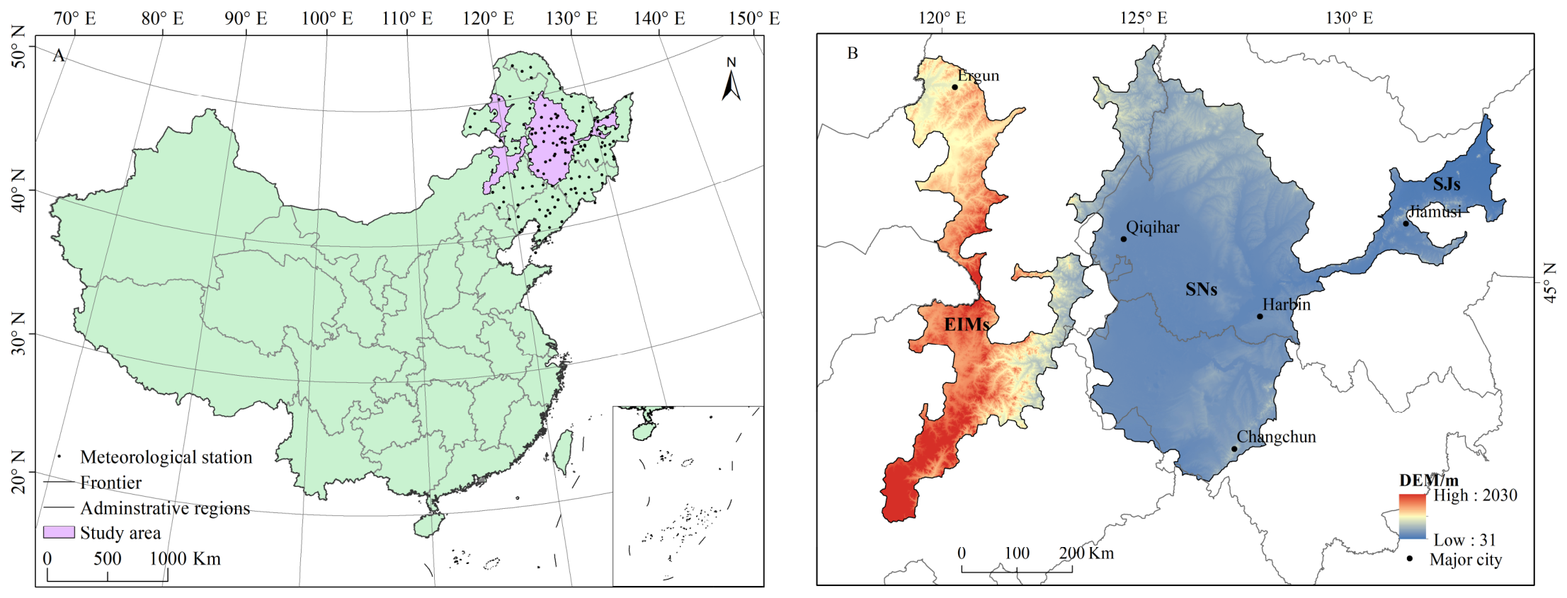
Figure 1. Location (A) and altitude (B) of the TBSR.
Land 15 01616 g001
Figure 2. Temporal changes in the SEM (A) and grade proportions in the TBSR from 1980 to 2020 (B). The fitted lines in (A) represent the regressions for the annual average SEM (0.023 t·ha−1·a−1) and the annual maximum SEM (1.349 t·ha−1·a−1) for the period after 1999, respectively. Grade I: ≤0.2 t·ha−1·a−1; Grade II: 0.2–0.5 t·ha−1·a−1; Grade III: 0.5–1.0 t·ha−1·a−1; Grade IV: 1.0–1.5 t·ha−1·a−1; Grade V: 1.5–2.0 t·ha−1·a−1; Grade VI: 2.0–5.0 t·ha−1·a−1; Grade VII: >5.0 t·ha−1·a−1.
Land 15 01616 g002
Figure 3. Spatial distribution of average SEM in the TBSR from 1980 to 2020 (A) and across different land-use types by decade (B). The error bars in (B) represent the standard deviations of SEM values across pixels within each land-use type.
Land 15 01616 g003
Figure 4. SEM trends in the TBSR from 1980 to 2020. Variations in SEM are categorized in Table 3 according to the Theil–Sen Median trend (β) and the Mann–Kendall test (Z) as follows: “significant degradation” (β ≥ 0.0005, Z > 1.96), “slight degradation” (β ≥ 0.0005, |Z| ≤ 1.96), “stability” (|β| < 0.0005, |Z| ≤ 1.96), and “slight improvement” (β ≤ −0.0005, |Z| ≤ 1.96).
Land 15 01616 g004
Figure 5. Spatial persistence of SEM across various land use types in the TBSR from 1980 to 2020 ((A), all land use types; (B), farmland; (C), forest; (D), grassland; (E), wetland; (F), bare). The persistence categories are defined in Table 4 and are based on combinations of the Hurst exponent (H), the Theil–Sen Median trend (β), and the Mann–Kendall test (Z): “persistence with significant degradation” (H > 0.5, β ≥ 0.0005, Z > 1.96), “persistence with slight degradation” (H > 0.5, β ≥ 0.0005, |Z| ≤ 1.96), “ persistence with stability” (H > 0.5, |β| < 0.0005, |Z| ≤ 1.96), “ persistence with slight improvement” (H > 0.5, β ≤ −0.0005, |Z| ≤ 1.96), “ non-persistence with slight degradation” (H < 0.5, β ≥ 0.0005, |Z| ≤ 1.96), “ non-persistence with stability” (H < 0.5, |β| < 0.0005, |Z|≤ 1.96), and “non-persistence with slight improvement” (H < 0.5, β < −0.0005, |Z| ≤ 1.96).
Land 15 01616 g005
Figure 6. Descriptive rescaling of individual q values for each environmental factor. (A) 2000, (B) 2001–2010, and (C) 2011–2020. Each sector represents the percentage of a specific factor’s q value relative to the total of all q values. “Climate” encompasses T (temperature), R (precipitation), and SS (sunshine duration), and is not an additional factor.
Land 15 01616 g006
Figure 7. Interaction between factors from 2000 to 2020: (A) 2000, (B) 2001–2010, and (C) 2011–2020. Each cell shows the explanatory power of the interaction between two factors, with color intensity indicating the strength of the interaction effect.
Land 15 01616 g007
Figure 8. Spatial distribution patterns of contributions to the SEM from the climate-driven (CC) and non-climatic components (NC) in the TBSR from 1980 to 2020. The six categories are determined by the directions of K for SEMCC and SEMNC, as outlined in Table 2.
Land 15 01616 g008
Table 1. Description and sources of data.
Description (Abbreviation)Spatial ResolutionTime RangeData Sources
SEM500 m1980–2020https://doi.org/10.1177/00368504251328206
T, R, and SS1 km1980–2020China’s National Meteorological Science Data Center (https://data.cma.cn/, accessed on 8 January 2024)
NDVI250 m2000–2020NASA LP DAAC (MODIS/Terra MOD13Q1) (https://ladsweb.modaps.eosdis.nasa.gov/, accessed on 10 March 2021)
POP1 km2000, 2010, 2020China’s Resource and Environmental Science Data Platform (https://www.resdc.cn, accessed on 18 April 2025)
GDP1 km2000, 2010, 2020China’s Resource and Environmental Science Data Platform (https://www.resdc.cn, accessed on 18 April 2025)
LUCC1 km2000, 2010, 2020China’s Resource and Environmental Science Data Platform (https://www.resdc.cn, accessed on 16 April 2025)
DEM500 mFABDEM (https://data.bris.ac.uk/data/dataset/s5hqmjcdj8yo2ibzi9b4ew3sn, accessed on 4 April 2025)
Slope500 mDerived from DEM using ArcGIS 10.2
Table 2. Relative contribution of climate change and non-climatic factors to SEM.
KRelative Contribution Rate (%)
CCNCClimate-Driven Component (CC)Non-Climatic Factors (NC)
CC&NC Increase>0>0 K SEM CC K SEM × 100 % K SEM N C K SEM × 100 %
CC Increase>0<0100.00.0
NC Increase<0>00100.0
CC&NC Decrease<0<0 K SEM CC K SEM × 100 % K SEM N C K SEM × 100 %
CC Decrease<0>0100.00.0
NC Decrease>0<00.0100.0
Table 3. SEM trends in the TBSR.
ZβSEM TrendRatio (%)
>1.96≥0.0005Significant degradation0.1
−1.96~1.96≥00.0005Slight degradation26.8
−1.96~1.96−0.0005~0.0005Stability67.2
−1.96~1.96<−0.0005Slight improvement4.6
Notes: Z is the statistic of the Mann–Kendall test. “Slight degradation”, “stability,” and “slight improvement” refer to non-significant trends (|Z| ≤ 1.96). β is the Theil-Sen Median slope. β ≥ 0.0005 indicates an upward trend in the SEM, signifying intensified erosion and soil degradation. β < −0.0005 indicates a downward trend, reflecting an improvement in soil conditions. β close to 0 indicates a stable trend. Proportions in this table are based on classified pixels only; water bodies and no-data pixels are excluded and account for the remaining percentage.
Table 4. Persistence of SEM based on trends and Hurst index.
HβZSEM Persistence TypeProportion of Area (%)
H > 0.5≥00.0005>1.96Persistence with significant degradation0.1
H > 0.5≥00.0005−1.96~1.96Persistence with slight degradation25.6
H > 0.5−0.0005~0.0005−1.96~1.96Persistence with stability64.1
H > 0.5<−0.0005−1.96~1.96Persistence with slight improvement4.6
H < 0.5≥00.0005−1.96~1.96Non-persistence with slight degradation1.3
H < 0.5−0.0005~0.0005−1.96~1.96Non-persistence with stability3.1
H < 0.5<−0.0005−1.96~1.96Non-persistence with slight improvement<0.1
Notes: Proportions in this table are based on classified pixels only; water bodies and no-data pixels are excluded and account for the remaining percentage.
Table 5. The q values of influencing factors at three periods.
YearAltitudeSlopeLUCCNDVIGDPPOPTRSS
20000.2820.3960.0370.0370.0410.1110.0910.0310.048
2001–20100.2600.3770.0330.0160.0800.0750.0980.0190.044
2011–20200.2980.3960.009 *0.012 *0.1370.0990.0820.0190.050
Notes: * indicates significance at p < 0.05; others are significant at p < 0.001.
Table 6. The maximum risk range of different environmental factors on SEM in different periods.
Factor20002001–20102011–2020
Type/RangeType/RangeType/Range
Elev/m1230~14301230~14301230~1430
Slope/°6~86~86~8
LUCCGrasslandWetlandGrassland
NDVI0.70~0.800.63~0.800.68~0.85
GDP/(¥10,000/km2)<26<63<32
POP/(p/km2)<22<40<19
T/°C0.4~1.40.8~1.81.0~2.0
R/mm336~399320~345366~433
SS/h2795~28562955~30492806~2890
Disclaimer/Publisher’s Note: The statements, opinions and data contained in all publications are solely those of the individual author(s) and contributor(s) and not of MDPI and/or the editor(s). MDPI and/or the editor(s) disclaim responsibility for any injury to people or property resulting from any ideas, methods, instructions or products referred to in the content.