SAR-Based Flood Detection and Agricultural Land Cover Vulnerability in the Loukkos Floodplain: Implications for Land Use Management in Larache Province, Morocco

Abstract

Flood events in agricultural floodplains reflect not only rainfall intensity but the vulnerability of the affected area at the moment of the event. This study examines the January–February 2026 flood in Larache Province, Morocco, through an integrated remote sensing workflow combining Sentinel-1 SAR, CHIRPS precipitation, and Dynamic World land cover in Google Earth Engine, processed via the rgee R package. Flood extent was mapped using SAR backscatter change detection and cross-checked against rainfall dynamics, yielding about 6660 ha of inundation (2.4% of the province), concentrated along the main Loukkos river corridor and adjacent floodplain around Ksar El Kebir, with smaller scattered patches to the south. Land cover was assessed across four temporal windows (spring 2025, pre-event, post-event, and spring 2026) to evaluate how the landscape entered the event and how it recovered. A significant share of normally cultivated land was in a bare-soil state before the flood, a condition that the literature associates with increased runoff. Post-flood analysis across 25 sample areas grouped into three geomorphic zones shows spatially uneven recovery, with cropland still below seasonal norms in spring 2026. These patterns are consistent with structural land-use conditions (wetland loss, intensive seasonal agriculture, drought-degraded soils) that may have amplified an already severe event. The findings support cover cropping, updated flood-hazard zoning, and targeted wetland restoration to reduce vulnerability in the Loukkos floodplain and comparable Mediterranean alluvial floodplains.

1. Introduction

This study is one of the first thematic applications developed within the Earth Observation (EO) Hub established under the TNE-GPSEducation project, a capacity-building initiative jointly carried out by Politecnico di Milano (POLIMI), the École Nationale Supérieure des Mines de Rabat (ENSMR) and the Université Internationale de Rabat (UIR) and concluded on 30 June 2025. Conceived as a long-term institutional platform—a living educational laboratory that moves from global knowledge to site-specific applications—the EO Hub structures its activities around a set of thematic pathways [1]. Flood detection and cropland-damage assessment in agricultural floodplains is one of the selected pathways, demonstrated here through the January–February 2026 event in the Loukkos plain (northern Morocco).

Flooding is among the most damaging natural hazards affecting agricultural regions worldwide, causing substantial economic losses, threatening food security, and contributing to long-term soil degradation [2,3]. Floods are primarily triggered by extreme or prolonged precipitation, although their severity is strongly influenced by antecedent soil moisture, topography, drainage characteristics, and land use. Recent studies indicate that climate change is increasing the intensity and frequency of extreme precipitation events, thereby amplifying flood hazards and associated socio-economic impacts, particularly in vulnerable agricultural floodplains where extensive cropland and settlements occupy low-lying areas [2,3,4].

Agricultural floodplains are particularly vulnerable because extensive croplands, settlements, and transport infrastructure are commonly concentrated within low-lying alluvial landscapes where floodwaters naturally accumulate. Consequently, understanding both the hydrometeorological drivers of floods and the characteristics of exposed landscapes is essential for improving flood risk assessment, disaster preparedness, and land-use planning [5].

In Morocco, recurrent flood events have increasingly affected northern and northwestern territories, where heavy rainfall rapidly translates into the inundation of farmland and settlements, generating significant environmental, social, infrastructural, and agricultural impacts [6]. Riverine and flash floods also generate major damage to crops, infrastructure, and livelihoods [2]. Northern and Western Morocco is particularly vulnerable, as shown by documented flood events in Tetouan [7], the Gharb Plain [4], and the Loukkos River basin. The Loukkos basin is especially exposed because the river flows across a gently sloping alluvial plain that favors the lateral expansion and persistence of floodwaters.

The winter of 2025–2026 in Morocco produced severe hydrometeorological disturbances with major environmental, agricultural, and socio-economic consequences. Prolonged and intense rainfall, associated with a succession of deep cold depressions, generated widespread flooding across several low-lying plains and downstream river sectors, particularly in the Gharb and Loukkos regions. These areas have previously been identified as highly susceptible to flooding because of their low-lying topography, dense hydrographic network, and concentration of agricultural land. In particular, flood hazard assessments have shown that a large proportion of the flood-prone areas in Larache Province exhibit moderate to high flood hazard levels [8], while climate risk assessments have identified the northwestern sector around Ksar El Kebir as one of the principal coastal flood-risk hotspots in northern Morocco [9]. As precipitation persisted over several weeks, soils progressively lost their infiltration capacity, promoting generalized surface runoff and the expansion of water over large areas. Seasonal wetlands, ponds, and marshes filled rapidly; river discharge increased markedly, and dam reservoirs approached critical storage levels.

The agricultural sector was among the most affected. Extensive tracts of farmland were inundated, causing major losses in cereals, sugar beet, vegetable crops, and soft fruit production. The concentration of Morocco’s most productive agricultural lands within the Gharb and Loukkos plains makes these regions particularly vulnerable to extreme rainfall and flooding, despite the generally beneficial role of rainfall for water resources and agriculture [10]. Beyond agriculture, the impacts extended to infrastructure and daily life: roads and bridges were damaged, mobility was disrupted, and access to basic services became difficult in several localities. Previous flood risk studies in northern Morocco have likewise highlighted the vulnerability of transport infrastructure and settlements located within flood-prone areas, emphasizing the potential for disruptions to connectivity and essential services during major flood events [8,9]. In several cases, settlements were temporarily isolated by floodwaters, with interruptions in electricity, drinking water supply, and road connectivity, leading to evacuations and population displacement.

Accurate and timely mapping of flood extent, duration, and recession is essential to quantify impacts on crops and to support disaster risk management, policy decisions and farmer preparedness [11]. Remote sensing and GIS technologies have proven effective for monitoring floods and assessing agricultural damage [12].

Sentinel-1 SAR satellite data provides high temporal resolution for flood extent mapping [13]. The use of Sentinel-1 (S1) radar for flood detection offers several critical advantages over traditional optical satellites and older radar missions, primarily due to its technical specifications and systematic acquisition policy [14]. It has global coverage, as it consists of a constellation of two satellites that can monitor the entire Earth every 6 days, acquiring data systematically with a stable incidence. As a Synthetic Aperture Radar (SAR) mission, Sentinel-1 can monitor land in almost all-weather conditions, including through dense cloud cover and rain and during the night [14]. This capability is a major advantage for flood mapping, as flooding is often caused by extreme weather events where clouds would hide or obscure the view of optical satellites [15].

Sentinel-1 also strongly supports big data and time-series analysis through its systematic and frequent acquisitions, which generate extensive image archives over time. These long-term series allow researchers to characterize normal backscatter conditions for each pixel under non-flooded conditions and identify anomalies caused by floods [16,17,18]. Access to multiple reference images also helps distinguish permanent low-backscatter surfaces, such as roads or airport runways, from floodwater [17]. In addition, Sentinel-1 data is openly and freely accessible through the European Space Agency (ESA), while its large data volume can be efficiently processed using cloud computing platforms such as Google Earth Engine (GEE) [18,19]. This cloud-based processing enables rapid management and analysis of large datasets, producing near-real-time results compared with older and more time-consuming manual methods [19].

Beyond inundation mapping, the literature shows that flood risk in Mediterranean and Moroccan floodplains is closely tied to land use, because exposed zones often combine cropland, low-lying corridors, and urbanized areas [20]. Agricultural loss has also been treated explicitly in recent crop-damage frameworks, from AGRIDE-c to Sentinel-based methods that estimate flood depth over crops [21]. For Morocco, the available evidence already includes Sentinel-1 flood mapping in Tetouan and flood-modelling work in northern Morocco, while neighboring basins show that flood events can affect crop fields, roads, and buildings [7]. These studies support the use of multi-temporal SAR and land-cover data to assess not only inundation extent but also the vulnerability of the Loukkos floodplain and its agricultural assets.

In the present study, these established techniques are used as reliable tools for the broader objective of evaluating flood impacts on agricultural systems rather than as methodological innovations only. This study investigates the flood event of February 2026 in Larache Province, Northern Morocco. An unsupervised Otsu-based thresholding and terrain filtering approach combined with multi-temporal Sentinel-1 SAR imagery is used to map flood extent, persistence and recession, which are then combined with cropland information to evaluate the agricultural exposure and post-flood recovery of the Loukkos floodplain.

Accordingly, this study addresses the following research questions:

• How effectively can multi-temporal Sentinel-1 SAR imagery delineate the spatial extent of the January–February 2026 flood in the Loukkos floodplain, in relation to the antecedent rainfall dynamics?
• How did the flood affect agricultural land cover and its seasonal recovery across the affected floodplain?
• How can integrating SAR-derived flood mapping with multi-temporal land-cover analysis support the assessment of agricultural exposure and flood-risk management in Mediterranean agricultural landscapes?

By addressing these questions, the study combines well-established SAR flood mapping techniques with an agricultural vulnerability perspective, providing actionable information for post-disaster management, agricultural resilience and climate adaptation in one of the most flood-prone agricultural areas in Morocco.

2. Materials and Methods

2.1. Study Area

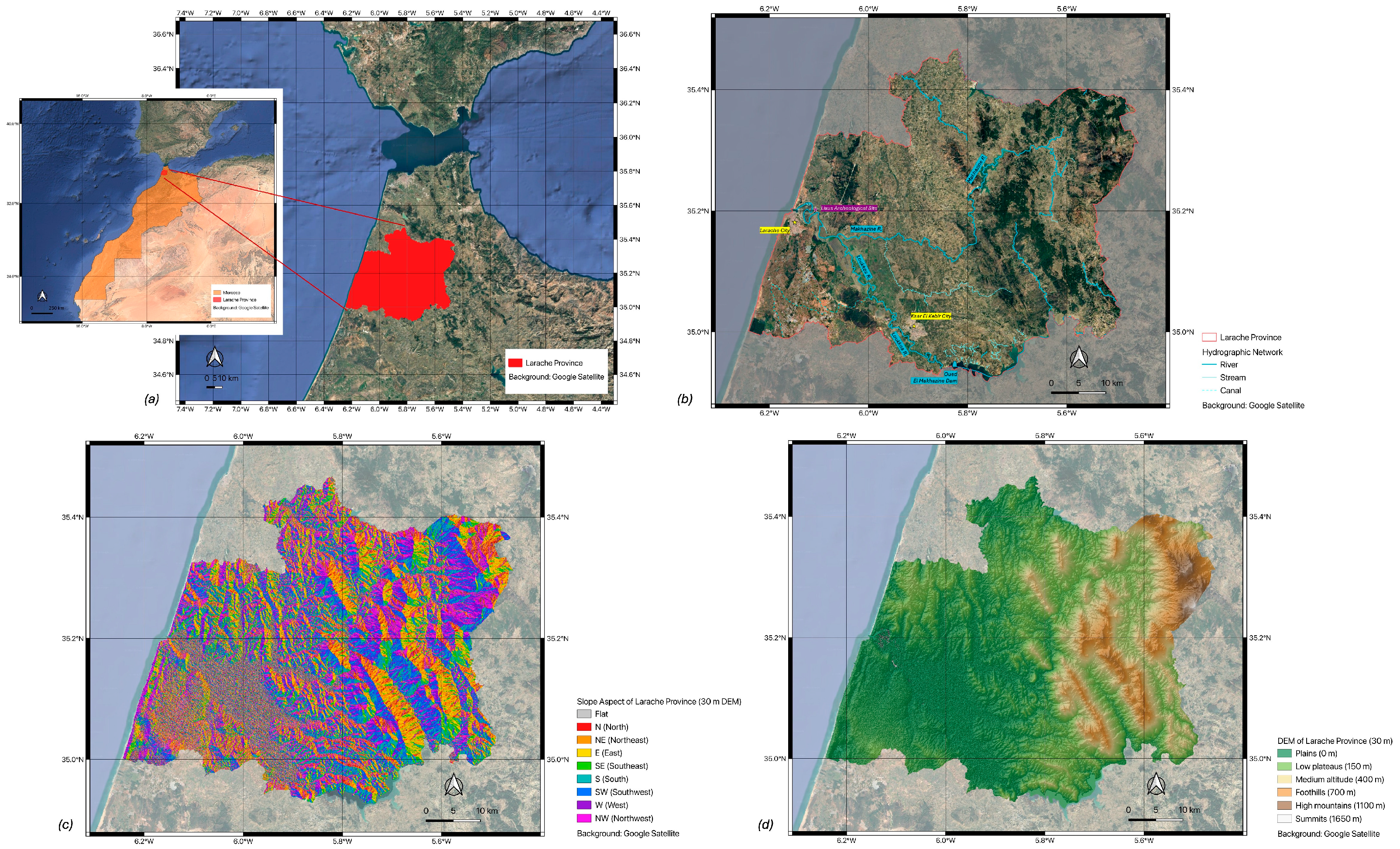
The Area of Interest (AOI) of the study is the province of Larache, located in the north of Morocco, along the Atlantic coast, within the Tangier-Tetouan-Al Hoceima region (Figure 1a). The province comprises 19 communes in total, including 2 urban communes (municipalities) and 17 rural communes.

The Loukkos Plain is among the most productive agricultural regions in northern Morocco, with Larache Province contributing substantially to its agricultural importance through its extensive irrigated lands and leading role in regional agricultural production [22]. The concentration of irrigated croplands and water resources also makes the area particularly sensitive to hydrological extremes associated with intense rainfall events [10]. The province covers an area of approximately 2684 km² and lies between 34°30′00″ and 35°10′00″ N and between 5°45′00″ and 6°30′00″ W. Elevation ranges from sea level to about 1650 m a.s.l. (Figure 1d), with slopes reaching up to 54° in the eastern reliefs, where the terrain also displays a marked variability in slope aspect (Figure 1c).

The Loukkos basin is structured around a major hydraulic installation, the Oued El Makhazine Dam (Figure 1b), one of Morocco’s most important dams [23]. Built on the Loukkos River, the dam stores upstream flows within a reservoir and regulates downstream discharge, serving primarily irrigation and water supply functions. Downstream from the dam, the Loukkos flows toward the Atlantic through a broad marshy depression, a geomorphological setting that contributes to the hydrological sensitivity of the lower valley. Within this fluvial system, Ksar El Kebir is located upstream of Larache within the low-lying alluvial plain of the middle-lower Loukkos valley, whereas Larache occupies a relatively elevated position on the cliffed left bank of the river mouth. Before the commissioning of the Oued El Makhazine Dam in 1979, flooding was a recurrent feature of the lower Loukkos system, with major floods inundating the coastal estuary and frequently affecting Ksar El Kebir [24,25]. Archaeological and geoarchaeological evidence further indicates a long-standing interaction between human settlement and the evolving fluvial and estuarine environment of the lower Loukkos valley [24].

Roman settlements and communication routes were strategically established on elevated ridges to avoid low-lying flood-prone areas. The ancient site of Lixus (Figure 1b), for instance, was built on a rocky hill approximately 80 m above sea level, allowing it to remain protected from seasonal inundation [26]. During major flood events, the surrounding plain reportedly became so submerged that the hill appeared as an island when viewed from the sea.

More recent archival evidence indicates that the estuarine zone was frequently inundated and that Ksar El Kebir experienced twelve flood episodes between 1936 and 1951 [27]. Far from representing an isolated or recent phenomenon, flooding is therefore closely linked to the geomorphological and hydrological functioning of the Loukkos valley. Although the construction of the Oued El Makhazine Dam significantly contributed to reducing flood hazards and regulating water resources within the basin, flood risk was not eliminated. 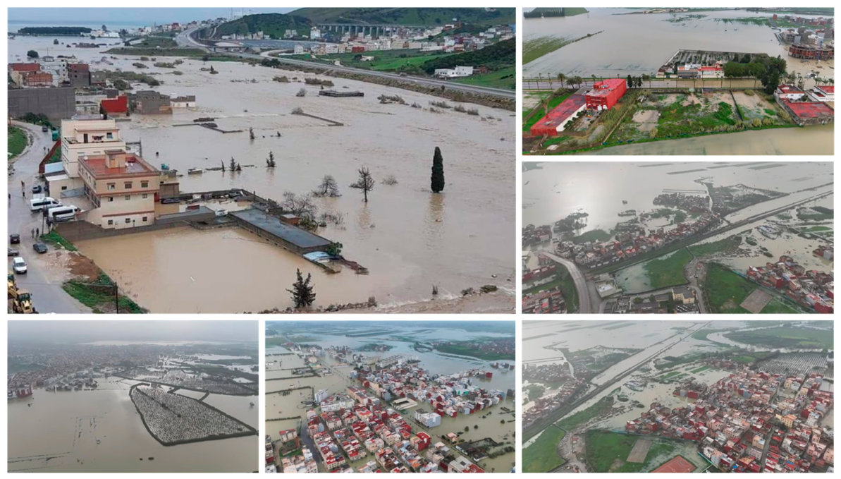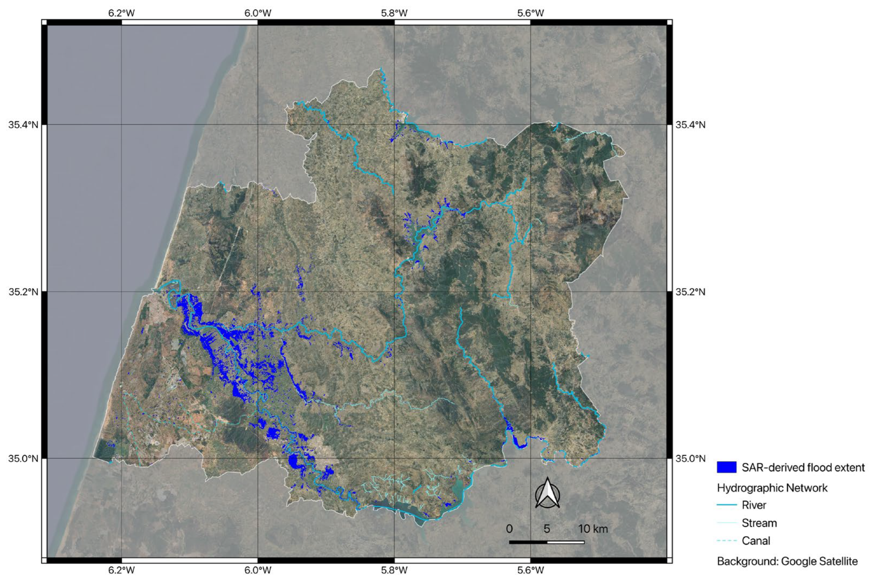Recent susceptibility assessments continue to identify the Ksar El Kebir–Larache floodplain among the most vulnerable sectors of the basin [28,29]. In this perspective, the February 2026 flood crisis (Figure 2), which triggered large-scale evacuations in Ksar El Kebir, appears less as an isolated disaster than as part of a long historical continuum of recurrent flooding, territorial adaptation, and persistent vulnerability within the lower Loukkos valley.

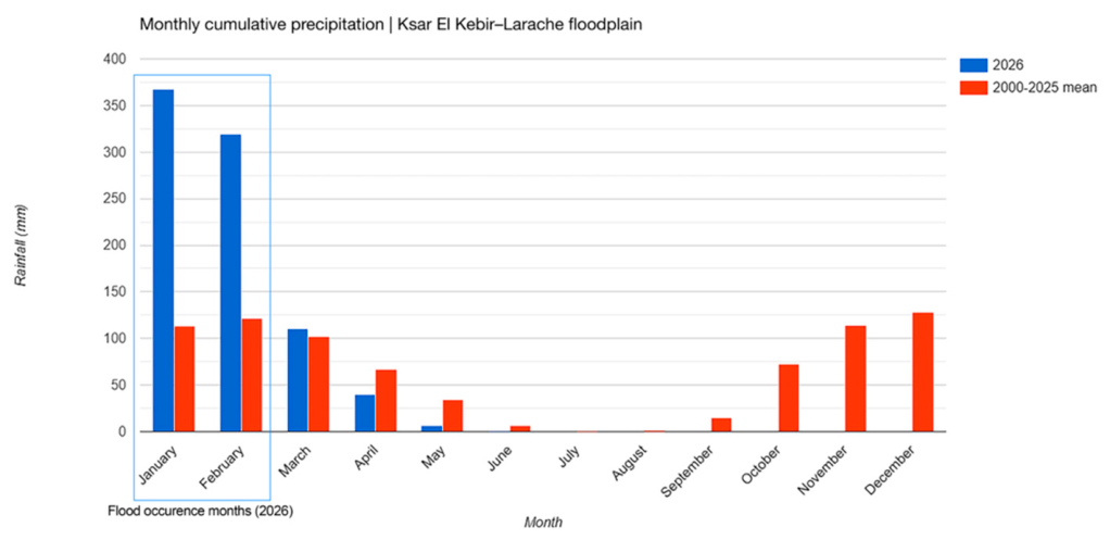
The climate is Mediterranean with strong Atlantic influences, characterized by mild, wet winters and warm, dry summers. To provide an introductory climatic context, the precipitation and temperature regime is described here for the Ksar El Kebir–Larache floodplain, the sector most affected by the January–February 2026 flood crisis. This analysis was conducted using the CHIRPS Daily Version 2.0 Final precipitation dataset and the ERA5-Land Daily Aggregated reanalysis dataset for the 2000–2025 period. 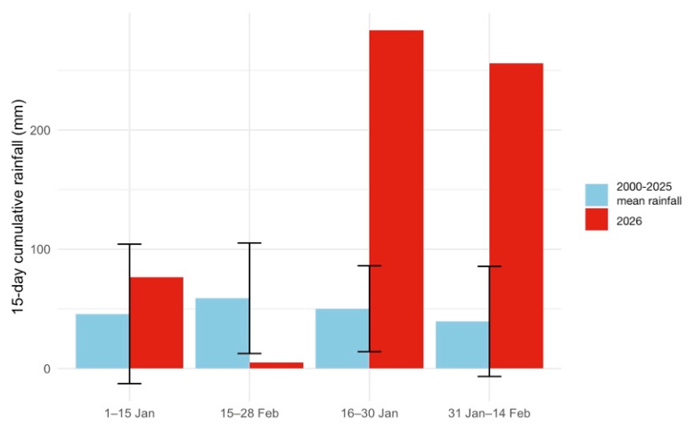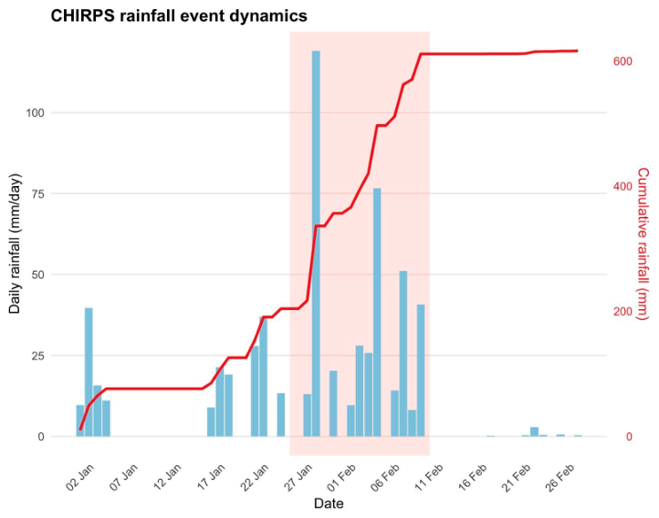The long-term monthly precipitation regime derived from CHIRPS (Figure 3) shows a pronounced wet season extending from October to April. Following the chronological progression of this wet season, monthly rainfall is already high in November (114.2 mm), peaks in December (128.5 mm), and remains substantial in January (113.0 mm) and February (121.7 mm), before declining markedly through late spring into a dry summer, when monthly precipitation averages less than 2 mm in July and August. Against this background, the 2026 hydrological season was exceptionally wet. Cumulative rainfall reached 367.5 mm in January and 318.9 mm in February, compared with long-term monthly means of 113.0 mm and 121.7 mm, respectively. The exceptionally high rainfall recorded during January and February coincided with the period of severe flooding, underscoring the magnitude of the hydroclimatic anomaly associated with the event. 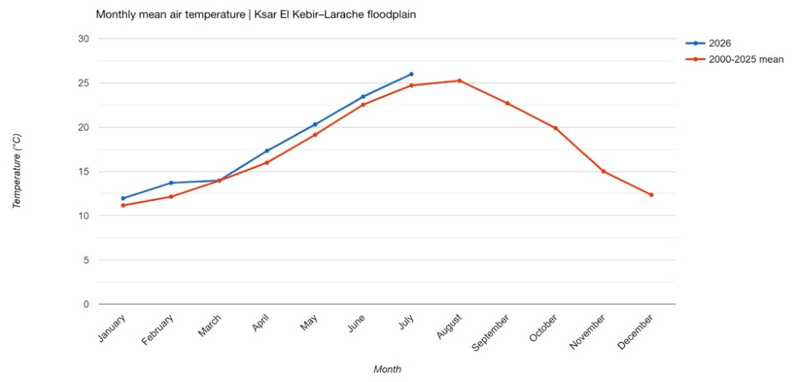The long-term monthly temperature regime (2000–2025) derived from ERA5-Land (Figure 4) reflects the typical Mediterranean climate of the region, with mean monthly temperatures increasing progressively from 11.2 °C in January to 25.2 °C in August, before declining towards winter. During the 2026 hydrological season, monthly mean temperatures remained close to the 2000–2025 average, though slightly above it between January and July. Mean temperatures reached 11.9 °C in January and 13.7 °C in February, compared with long-term means of 11.2 °C and 12.1 °C, respectively. Similarly, mean daily minimum temperatures were 9.4 °C and 10.1 °C, while mean daily maximum temperatures were 14.8 °C and 17.9 °C in January and February, respectively. Overall, temperature conditions during the flood period remained within the range of normal interannual variability, indicating that the exceptional hydroclimatic conditions of early 2026 were primarily associated with anomalously high precipitation rather than unusual thermal conditions.

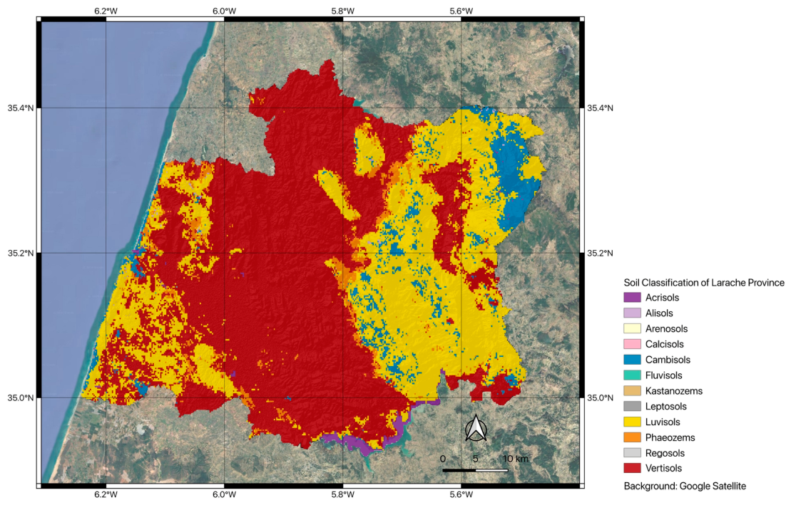
The geological and pedological setting of the area further conditions its hydrological response. Geologically, Larache Province is mainly composed of Cretaceous and Tertiary deposits, with alluvial plains along the Oued Loukkos [31,32]. The soils of the study area were characterized using the global SoilGrids database (~250 m resolution; [33]). The regional soil cover is dominated by clay-rich soils (Figure 5): Vertisols, characterized by a high content of expandable clays and pronounced shrink–swell behaviour, occupy most of the plain, alongside Luvisols, fertile soils marked by subsurface clay accumulation. These are locally associated with Cambisols (weakly developed brown soils), Phaeozems (dark, humus-rich meadow soils) and, more marginally, Acrisols (acidic soils with clay illuviation and low base saturation). The predominance of clay-rich Vertisols and Luvisols is particularly relevant to flood dynamics, since their infiltration capacity is strongly moisture-dependent and their surfaces are prone to sealing and crusting when left bare—conditions that can enhance runoff generation during intense rainfall [34,35].

2.2. Data Sources

This study adopts an integrated multi-sensor workflow combining multi-temporal precipitation data, Synthetic Aperture Radar (SAR) observations, and satellite-derived land cover information, based on the joint use of rainfall data from CHIRPS, C-band SAR data from the European Space Agency Sentinel-1 mission, and land cover products from Dynamic World. All datasets were accessed and processed within the Google Earth Engine (GEE) environment through the rgee package in R [36]. The Area of Interest (AOI) of this study is Larache Province; the datasets and the temporal windows used are summarized in

Table 1. Datasets and temporal windows used in the analysis.

Dataset	Product/Source	Spatial Resolution	Role/Variable	Temporal Window
CHIRPS	CHIRPS Daily v2.0	~5 km	Mean 2000–2025 rainfall vs. 2026	1 January–28 February 2000–2025
CHIRPS	CHIRPS Daily v2.0	~5 km	Daily rainfall; event-window identification	1 January–28 February 2026
Sentinel-1 (reference)	GRD, IW, VV+VH, descending	10 m	Pre-event backscatter baseline	15–24 January 2026 (5 scenes)
Sentinel-1 (event)	GRD, IW, VV+VH, descending	10 m	Flood detection	25 January–10 February 2026 (6 scenes)
Dynamic World	Sentinel-2, deep learning	10 m	Land cover—spring growing season baseline	March–May 2025
Dynamic World	Sentinel-2, deep learning	10 m	Land cover—pre-event baseline	October–November 2025
Dynamic World	Sentinel-2, deep learning	10 m	Land cover—post-event	January–February 2026
Dynamic World	Sentinel-2, deep learning	10 m	Land cover—spring growing season recovery	March–May 2026

.

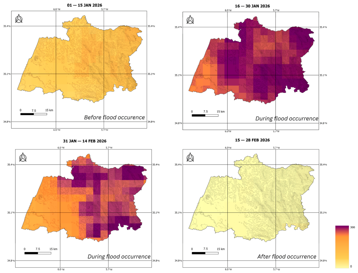
The Climate Hazards Group InfraRed Precipitation with Stations (CHIRPS) dataset integrates satellite-based infrared observations with in situ rain gauge measurements to provide quasi-global precipitation estimates, particularly suited for regions with limited ground-based monitoring [37]. The product used here is CHIRPS Daily version 2.0 (GEE asset UCSB-CHG/CHIRPS/DAILY), with a spatial resolution of approximately 0.05° (~5 km) and a daily temporal resolution. The variable considered is daily precipitation, P(x,t) [mm/day], where x denotes the spatial location and t the temporal dimension. The analysis was carried out over the AOI for January–February 2026, corresponding to the pre-event and event/post-event phases of the flood; in addition, the 2026 cumulative rainfall of each 15-day interval was compared with the corresponding 2000–2025 long-term average from CHIRPS to place the event in a climatological context.

The Sentinel-1 mission provides C-band SAR data acquired in Interferometric Wide Swath (IW) mode, with a spatial resolution of approximately 10 m and a revisit time of 6–12 days depending on orbital configuration [14]. SAR data are particularly suitable for flood detection due to their sensitivity to surface roughness and dielectric properties and their capability to operate independently of cloud cover and illumination conditions [15]. Ground Range Detected (GRD) products with dual polarization (VV+VH) were used, all in descending orbit, with a specific focus on the VH channel, which is more responsive to surface-water-induced backscatter reductions [17]. The GEE COPERNICUS/S1_GRD collection is supplied already preprocessed with the standard Sentinel-1 Toolbox chain (precise orbit file, border- and thermal-noise removal, radiometric calibration to the backscatter coefficient σ° in dB, and range-Doppler terrain correction using the SRTM DEM).

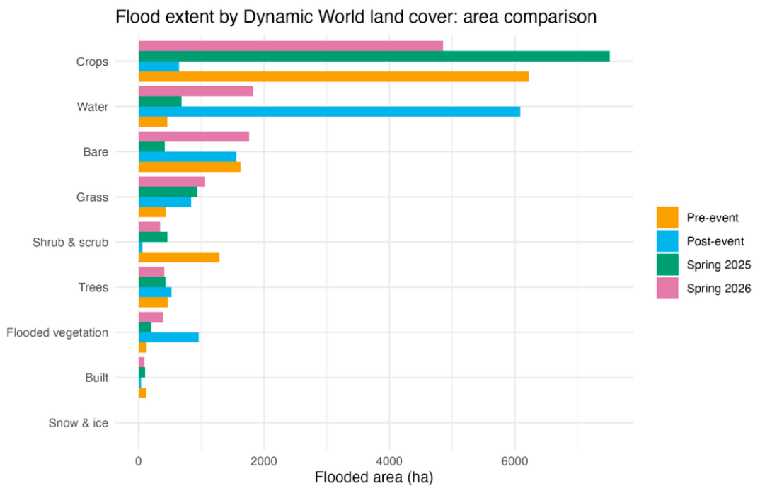
Land cover information was derived from Dynamic World, a near-real-time global land cover product at 10 m resolution generated from Sentinel-2 imagery using a deep-learning framework [38], comprising nine classes (water, trees, grass, flooded vegetation, crops, shrub and scrub, built area, bare ground, and snow/ice). Categorical maps were produced as the modal class over four temporal windows: a spring growing-season baseline (March–May 2025) and a pre-event baseline (October–November 2025), both representing non-flooded reference conditions; the event/post-event window (January–February 2026); and the spring growing season 2026 (March–May 2026), used to assess post-flood recovery.

2.3. Methods

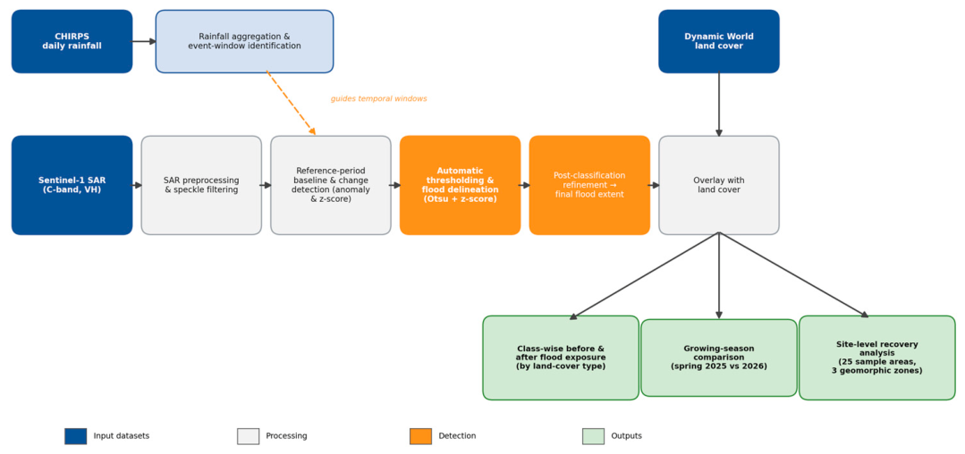
This study adopts a sequential, data-driven workflow (Figure 6) that integrates the precipitation, SAR, and land-cover datasets described in Section 2.2 to characterize flood dynamics and their interaction with surface conditions. Antecedent CHIRPS rainfall is aggregated to identify the flood event window, which in turn guides the temporal windows of the Sentinel-1 processing chain; VH backscatter is preprocessed and speckle-filtered, and a reference-period baseline supports event-versus-baseline change detection, which is thresholded and refined (noise removal and terrain masking) to delineate the final flood extent. Overlay with Dynamic World land cover then yields the class-wise flood exposure by land-cover type, the growing-season comparison (spring 2025 vs. 2026), and the post-flood recovery analysis across the 25 sample areas. The individual steps are detailed in the following subsections.

Precipitation patterns are first analyzed to identify critical temporal windows associated with hydrological response, which are subsequently used to guide SAR-based flood detection. Daily precipitation data from the CHIRPS dataset were analyzed over the period 1 January–28 February 2026, capturing both pre-conditioning and peak rainfall phases in the Larache Province. To characterize rainfall accumulation, the study period was subdivided into four consecutive 15-day intervals. For each interval t, cumulative precipitation was computed (as shown in Formula (1)):

$$P_{\mathrm{c}\mathrm{u}\mathrm{m}}(t)={\displaystyle \sum _{k=1}^n}{R}_k$$

(1)

where $R_k$ represents daily rainfall (mm) and n = 15 days. This metric captures the temporal integration of precipitation and serves as a proxy for hydrological loading, commonly used to interpret runoff generation processes [39]. For each interval, spatial statistics including minimum, maximum, mean, and 95th percentile were derived over the Area of Interest (AOI), with the latter used to characterize high-intensity rainfall while limiting sensitivity to outliers. A daily rainfall time series was also computed by spatially averaging precipitation over the AOI, enabling the identification of rainfall peaks and cumulative hydrological loading preceding flood occurrence. The 2026 rainfall was also compared with the 2000–2025 CHIRPS 15-day cumulative rainfall for every year from 2000 to 2025; the resulting climatological mean and standard deviation were then used to express the 2026 values both as absolute anomalies (2026 minus the long-term mean) and as ratios to that mean.

In Sentinel-1 SAR imagery, VH polarization is particularly sensitive to volume scattering. Although VH is generally more affected by noise [40], flood detection can still be effectively implemented using anomaly-based approaches applied to VH polarization time series, where deviations from baseline backscatter conditions indicate potential inundation. To distinguish flooded from non-flooded areas, several automated thresholding techniques have been developed, among which Otsu’s method [41] is one of the most widely used. Otsu’s method is an automatic image-thresholding algorithm that has demonstrated strong performance in SAR-based flood detection, particularly when combined with multi-temporal change detection approaches [16,42]. Its effectiveness, combined with dense Sentinel-1 time-series data, makes it well suited for fully automated flood mapping in large-scale and complex environments [15,17,43]. Drawing on these established approaches, the present study implements an anomaly-based, Otsu-thresholded methodological workflow on multi-temporal Sentinel-1 VH data to map the January–February 2026 flood in the Loukkos plain, as detailed below.

Flood extent was derived from Sentinel-1 C-band SAR data using this multi-temporal anomaly-based approach. GRD images acquired in Interferometric Wide Swath (IW) mode and VH polarization were selected over a pre-event reference period (15–24 January 2026) and an event window (25 January–10 February 2026), defined based on rainfall dynamics. In total, 5 GRD scenes were used for the reference period and 6 for the event window, all in descending orbit and dual polarization (VV+VH); the full scene inventory and product identifiers are listed in

Table 2. Sentinel-1 GRD scenes used for the pre-event reference period (15–24 January 2026). All scenes: IW mode, descending orbit, dual polarization (VV+VH).

Product ID	Date (UTC)	Platform	Rel. Orbit
S1C_IW_GRDH_1SDV_20260116T062656_20260116T062721_005925_00BE1A_A35D	2026-01-16 06:26	S1C	154
S1A_IW_GRDH_1SDV_20260117T061927_20260117T061952_062803_07E08D_31B4	2026-01-17 06:19	S1A	81
S1A_IW_GRDH_1SDV_20260117T061952_20260117T062017_062803_07E08D_3F9F	2026-01-17 06:19	S1A	81
S1A_IW_GRDH_1SDV_20260122T062746_20260122T062811_062876_07E31A_3889	2026-01-22 06:27	S1A	154
S1C_IW_GRDH_1SDV_20260123T061846_20260123T061911_006027_00C159_6E68	2026-01-23 06:18	S1C	81

(reference period) and

Table 3. Sentinel-1 GRD scenes used for the event window (25 January–10 February 2026). All scenes: IW mode, descending orbit, dual polarization (VV+VH).

Product ID	Date (UTC)	Platform	Rel. Orbit
S1C_IW_GRDH_1SDV_20260128T062655_20260128T062720_006100_00C3CC_346B	2026-01-28 06:26	S1C	154
S1A_IW_GRDH_1SDV_20260129T061926_20260129T061951_062978_07E6DD_A7A0	2026-01-29 06:19	S1A	81
S1A_IW_GRDH_1SDV_20260129T061951_20260129T062016_062978_07E6DD_F30C	2026-01-29 06:19	S1A	81
S1A_IW_GRDH_1SDV_20260203T062746_20260203T062811_063051_07E997_9846	2026-02-03 06:27	S1A	154
S1C_IW_GRDH_1SDV_20260204T061845_20260204T061910_006202_00C743_2DF9	2026-02-04 06:18	S1C	81
S1C_IW_GRDH_1SDV_20260209T062655_20260209T062720_006275_00C9C2_CF76	2026-02-09 06:26	S1C	154

(event window). SAR-based flood detection relies on the strong contrast between open water and surrounding surfaces, where smooth water bodies induce a marked decrease in backscatter due to specular reflection [39,44]. VH polarization has been shown to enhance the detection of inundated areas and improve class separability, particularly in heterogeneous and vegetated environments [45]. The cross-polarized VH channel is dominated by volume scattering and is more sensitive than co-polarized VV to the scattering loss caused by the specular reflection of smooth open water, so it yields a larger and more consistent backscatter drop over inundated land and better separates flooded from non-flooded surfaces in the heterogeneous, partly vegetated Loukkos agricultural mosaic. To confirm this choice for the study site, the identical detection workflow was run in three configurations (VH-only, VV-only, and the VH+VV intersection): VV-only over-detected the flooded area (9577.47 ha, ~44% larger than VH), consistent with the sensitivity of the co-polarized channel to residual surface roughness over non-flooded parcels, whereas the VH+VV intersection was conservative (5351.25 ha, ~20% smaller), omitting shallow or vegetated inundation; VH-only (6657.57 ha) produced spatially coherent flood extent, aligned with the drainage network and low-lying floodplain. VH was therefore adopted as the operational channel, with VV and VH+VV retained only for comparison. For the comparison, the VV channel was thresholded with the same Otsu-plus-z-score procedure (Otsu anomaly threshold capped at −1.5 dB; z-score cut-off −1.3); these values apply only to the VV and VH+VV comparison and not to the final VH-based product.

Multi-temporal SAR analysis enables the detection of flood-induced changes by comparing event conditions against pre-event baseline states and has been widely applied for rapid flood mapping in complex environments [46,47,48] and in operational early warning frameworks [49]. For each period, SAR image collections were aggregated using the median to reduce scene-specific variability, and a focal median filter (60 m radius) was applied to mitigate speckle noise while preserving spatial structures.

A pre-event baseline was constructed by computing the mean and standard deviation of the VH backscatter signal (as shown in Formulas (2) and (3)):

$${\mu }_{\mathrm{V}\mathrm{H}}(x)={\displaystyle \frac{1}{N_R}}{\sum }_{t\in R}{\sigma }_{\mathrm{V}\mathrm{H}}^0(x,t)$$

(2)

$$s_{\mathrm{V}\mathrm{H}}(x)=\sqrt{{\displaystyle \frac{1}{N_R-1}}{\sum }_{t\in R}{\left[{\sigma }_{\mathrm{V}\mathrm{H}}^0(x,t)-{\mu }_{\mathrm{V}\mathrm{H}}(x)\right]}^2}$$

(3)

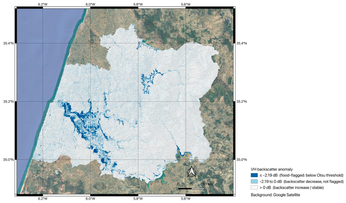
where N is the number of pre-event (reference-period) Sentinel-1 acquisitions. Here μ_VH denotes the baseline mean VH backscatter and s_VH the baseline standard deviation of VH backscatter—a quantity distinct from the backscatter coefficient ${\sigma }^0$itself; to avoid division by near-zero variability in the z-score, a floored standard deviation s*_VH = max(s_VH, 0.05) is used. The event backscatter, taken as the per-pixel temporal median over the event window, was compared to baseline conditions to derive the anomaly (Formula (4)):

$$A_{\mathrm{V}\mathrm{H}}\left(x\right)={\sigma }_{\mathrm{V}\mathrm{H},\mathrm{E}}^0\left(x\right)-{\mu }_{\mathrm{V}\mathrm{H}}\left(x\right)$$

(4)

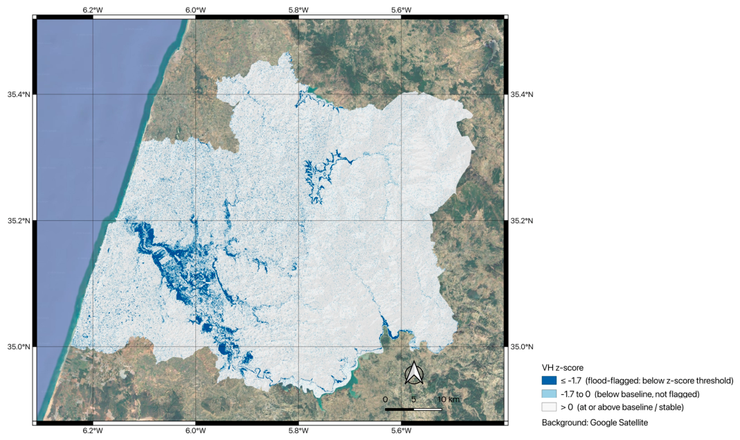
and standardized using a z-score (Formula (5)):

$$Z_{\mathrm{V}\mathrm{H}}(x)={\displaystyle \frac{A_{\mathrm{V}\mathrm{H}}\left(x\right)}{s_{\mathrm{V}\mathrm{H}}^{*}\left(x\right)}}$$

(5)

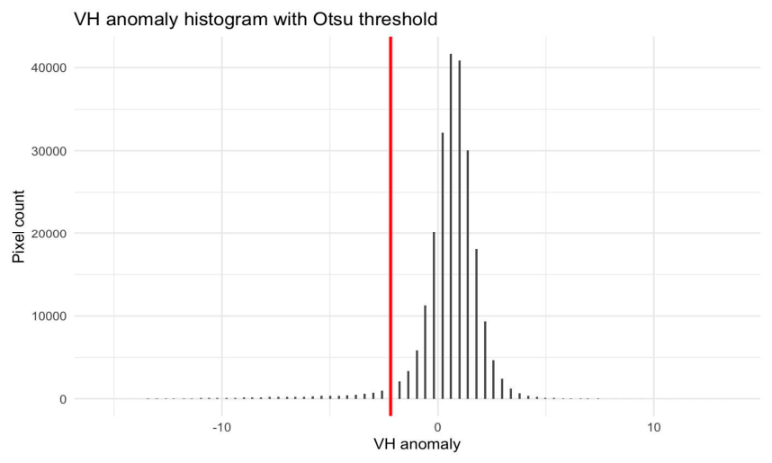
An adaptive threshold was applied to the anomaly distribution using Otsu’s method [41], which selects the anomaly value T that maximizes the between-class variance of the anomaly histogram (Formula (6)):

$$T=\arg \underset{\tau }{\max }\hspace{0.17em}{\omega }_0\left(\tau \right)\hspace{0.17em}{\omega }_1\left(\tau \right)\hspace{0.17em}{\left[{\mu }_0\left(\tau \right)-{\mu }_1\left(\tau \right)\right]}^2, T=-2.19\mathrm{d}\mathrm{B}$$

(6)

where τ is a candidate threshold scanned across the VH-anomaly histogram; ω₀(τ) and ω₁(τ) are the probabilities (pixel-count fractions) of the two classes—non-flooded and flooded—defined by τ; and μ₀(τ) and μ₁(τ) are the mean anomaly values of those two classes. The resulting data-driven threshold separates flooded from non-flooded pixels. 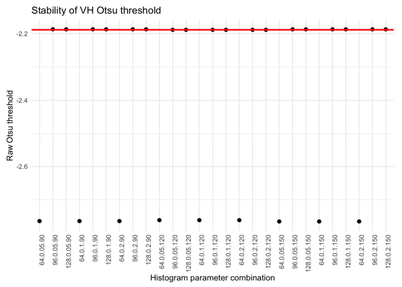Histogram-based thresholding approaches are adopted in SAR flood mapping due to their robustness and effectiveness [44,45]. To ensure conservative detection, the threshold was constrained to at most −2.0 dB, yielding an operational value of T = −2.19 dB. In this case the Otsu procedure returned −2.19 dB directly, so the −2.0 dB constraint was not binding and serves only as a safeguard for scenes where flooding occupies a negligible fraction of the AOI; open-water inundation characteristically produces backscatter reductions of several decibels relative to dry conditions. This anomaly threshold was combined with a z-score condition (a conservative empirical cut-off Z_thr = −1.7, approximately 1.7 standard deviations below the pixel-wise baseline mean) through a logical AND, so that a pixel is flagged as flooded only where the anomaly falls below T and the z-score falls below Z_thr, isolating strong backscatter reductions associated with inundation. Flooded pixels were defined as (Formula (7)):

$$F\left(x\right)=\left\{\begin{array}{ll}1,& A_{\mathrm{V}\mathrm{H}}\left(x\right)<T\hspace{0.25em}\wedge \hspace{0.25em}{Z}_{\mathrm{V}\mathrm{H}}\left(x\right)<Z_{\mathrm{t}\mathrm{h}\mathrm{r}}\\ 0,& \mathrm{otherwise}\end{array}\right. T=-2.19\mathrm{d}\mathrm{B},Z_{\mathrm{t}\mathrm{h}\mathrm{r}}=-1.7$$

(7)

The resulting flood mask was refined through light spatial filtering. A morphological filter was applied to reduce isolated noise, followed by connected pixel analysis retaining only clusters with at least five connected pixels. A slope-based constraint derived from the SRTM digital elevation model was then applied, retaining only areas with slope values below 6°. This slope mask removes steep hillslopes (slopes in the AOI reach 54°) where SAR layover and shadow degrade backscatter reliability and where standing floodwater is geomorphologically implausible, while retaining the near-flat alluvial floodplain where inundation occurs. The robustness of the VH anomaly threshold was evaluated through a sensitivity analysis by varying histogram construction parameters, including the number of bins (64–128), minimum bucket width (0.05–0.2), and spatial aggregation scale (90–150 m).

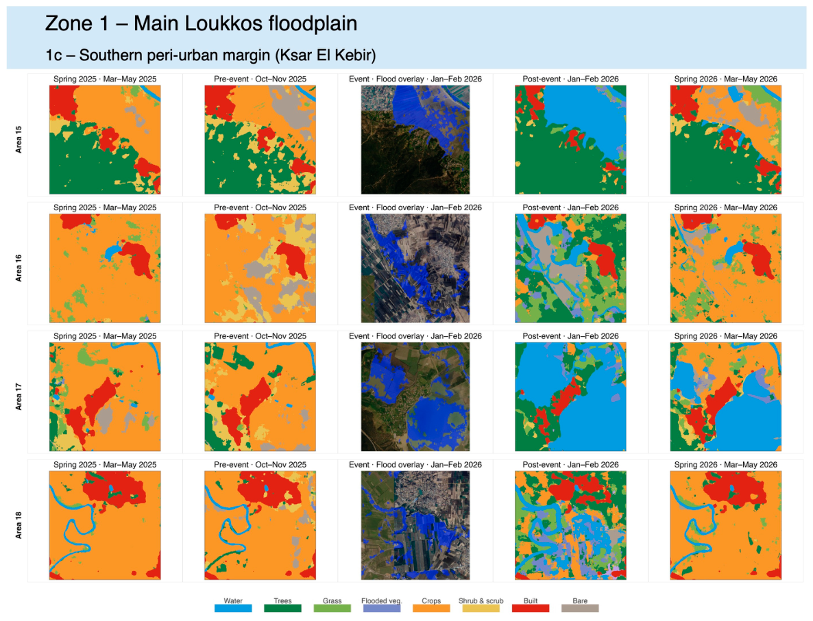
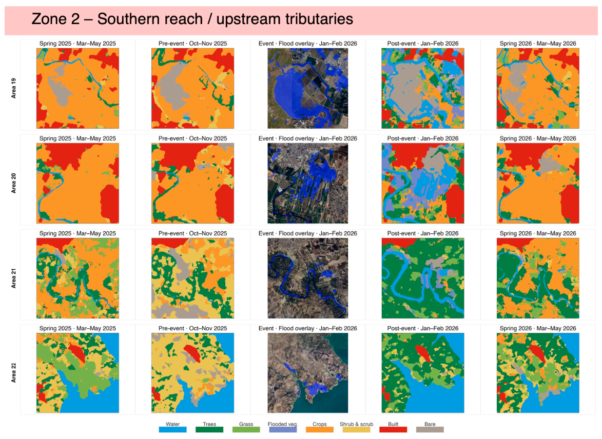
Finally, the SAR-derived flood mask is combined by spatial overlay (pixel-wise intersection on a common 10 m grid) with Dynamic World land cover data. Land cover maps were generated using the modal class over four temporal windows: spring growing season 2025 (March–May 2025), pre-event baseline (October–November 2025), event/post-event conditions (January–February 2026), and spring growing season 2026 (March–May 2026). The use of temporally aggregated land cover products reduces classification noise and improves the stability of land surface representation under dynamic environmental conditions [46]. The flood mask was applied to each land cover layer (Formula (8)):

$$A_{\mathrm{f}\mathrm{l}\mathrm{o}\mathrm{o}\mathrm{d}}\left(c\right)={\sum }_{x}F\left(x\right)\hspace{0.17em}\mathbb{1}\left\{L\left(x,t\right)=c\right\}\hspace{0.17em}a\left(x\right)$$

(8)

allowing the computation of class-wise flooded area and percentage and enabling a comparative assessment of flood exposure across land cover types and temporal conditions. Formally, land cover and flood extent are combined by spatial overlay—a pixel-wise intersection on a common 10 m grid, rather than fusion during classification. Let L(x,t) denote the Dynamic World categorical land-cover label (modal class) at pixel x for temporal window t, and a(x) the pixel area; for each land-cover class c the flooded area is A_flood(c) = Σ_x F(x)·𝟙{L(x,t) = c}·a(x), where F(x) is the binary flood mask (1 = flooded) and 𝟙{·} is the indicator function. This indicator formulation replaces the multiplication of categorical class codes by the flood mask, which is not formally valid for a nominal variable, and corresponds directly to the class-level statistics.

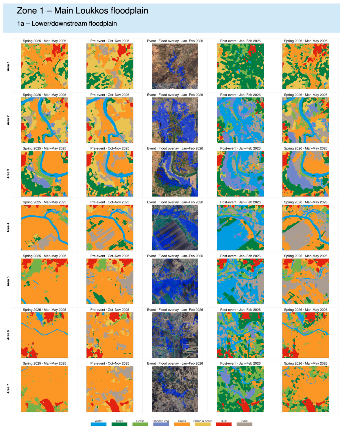
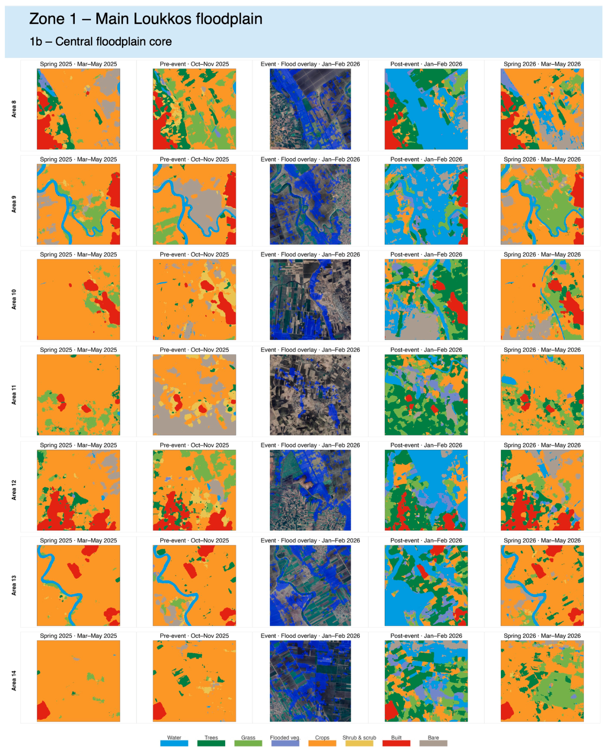
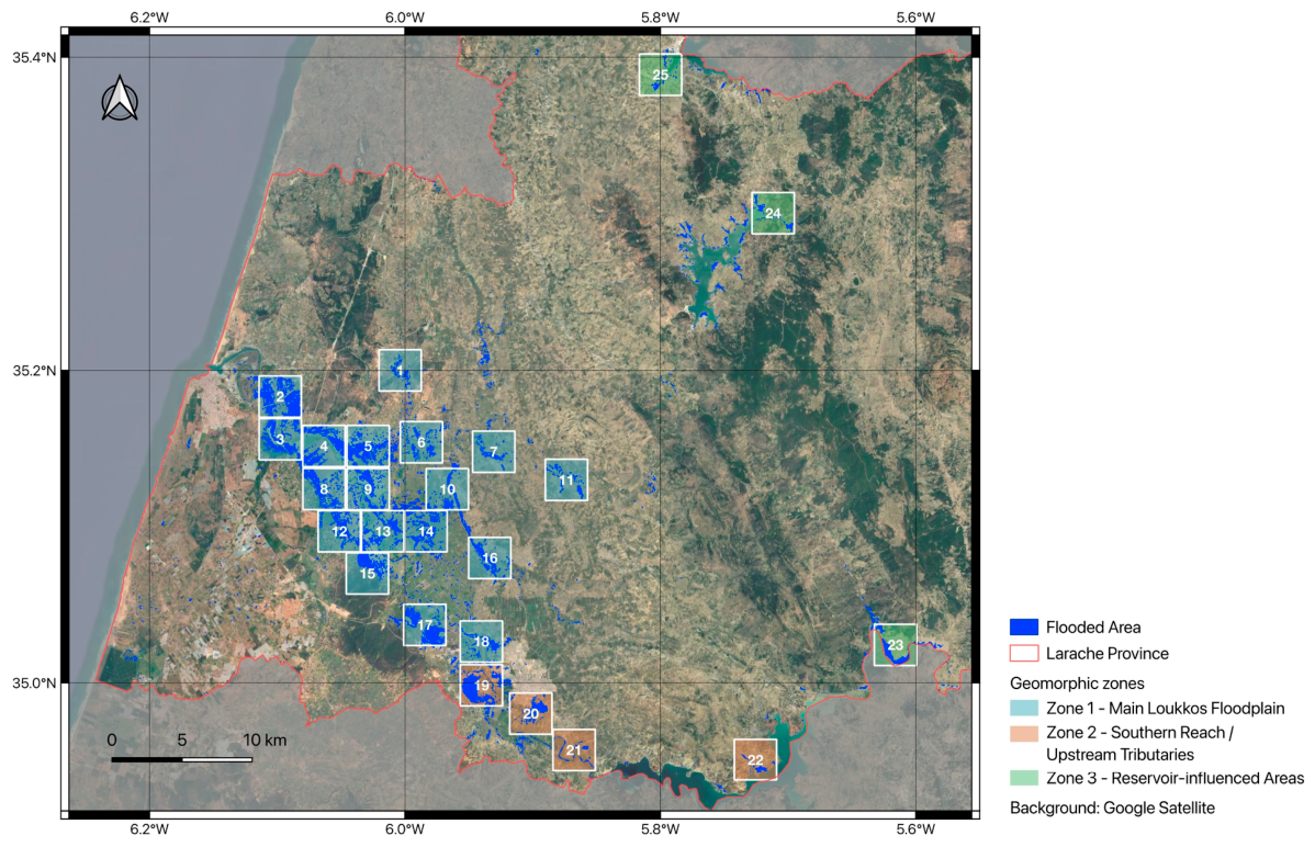
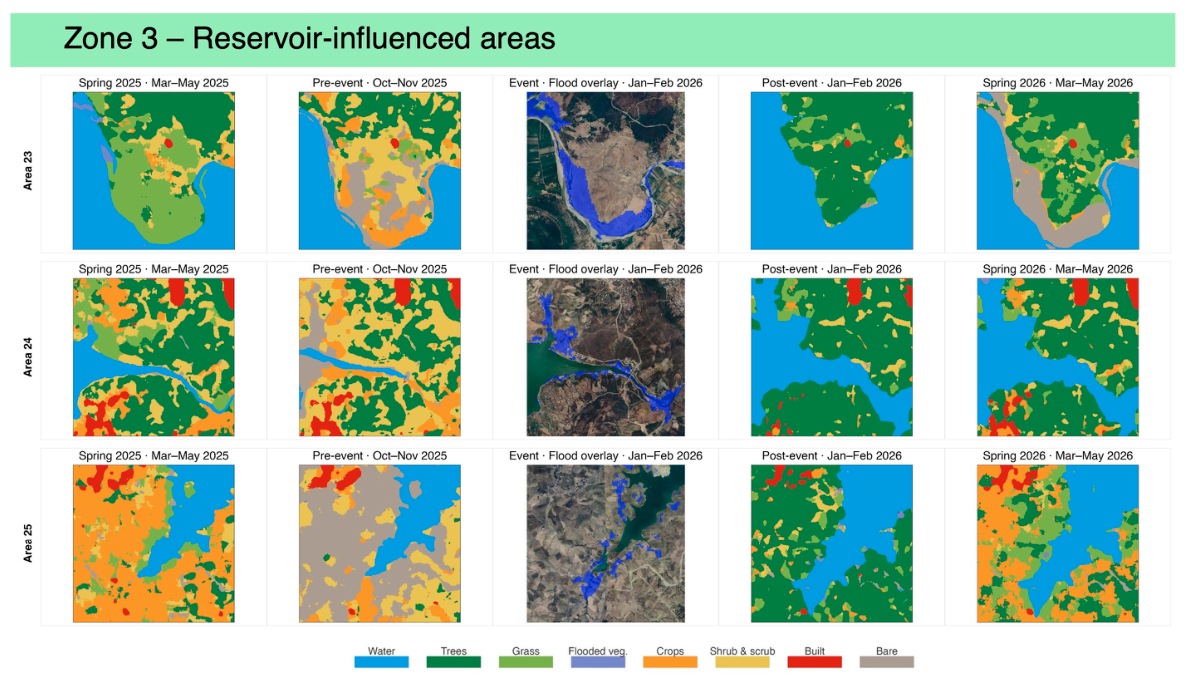
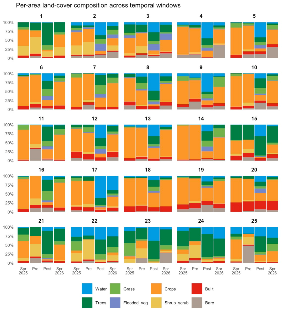
A site-level analysis was conducted across 25 sample areas spatially distributed throughout the SAR-derived flood footprint. Sample areas were delineated as square polygons of approximately 9 km² and selected to provide coverage of the full range of flood intensities, land cover types, and positions relative to the Loukkos River corridor documented within the study domain. For each area, Dynamic World land cover maps were extracted for the same four temporal windows used in the area-wide analysis: pre-event baseline (October–November 2025), event/post-event (January–February 2026), spring growing season 2025 (March–May 2025), and spring growing season 2026 (March–May 2026). Each area is visualised as a five-panel composite displaying the SAR-derived flood overlay on the satellite image alongside the four temporal land cover maps, enabling direct visual comparison of land surface conditions before, during, and after the flood event across spatially contrasting settings.

3. Results

The results of the workflow are presented through a multi-scale analysis integrating precipitation patterns, SAR-derived flood extent, and land cover information. Rainfall dynamics are first quantified to identify the temporal windows associated with peak hydrological forcing. These intervals are subsequently used to interpret SAR backscatter anomalies and derive flood extent. Finally, the integration with Dynamic World land cover data enables the quantification of flood exposure across different surface classes, providing insight into the spatial distribution of flood impacts.

3.1. CHIRPS Rainfall Aggregation and 15-Day Interval Statistics

The 15-day rainfall aggregation highlights a clear temporal variability in precipitation across the study period, with a strong concentration of rainfall during late January and early February 2026 (

Table 4. Rainfall statistics for 15-day intervals derived from CHIRPS over the study area. Minimum (Min), maximum (Max), mean (Mean), and 95th percentile (P95) precipitation values are reported for each period (mm per 15-day interval).

Period	Min (mm)	Max (mm)	Mean (mm)	P95 (mm)
1–15 January 2026	54.84	97.77	76.42	91.64
16–30 January 2026	234.94	352.76	283.50	321.71
31 January–14 February 2026	145.83	367.28	255.92	310.23
15–28 February 2026	2.73	18.95	5.02	7.17

). Rainfall conditions during the first interval (1–15 January) were moderate, with a mean precipitation of 76.42 mm and limited spatial variability (P95 = 91.64 mm). A substantial increase occurred in the second interval (16–30 January), representing the peak rainfall phase, with mean values reaching 283.50 mm and maximum values exceeding 350 mm. The high P95 (321.71 mm) indicates widespread high-intensity rainfall across the AOI. The third interval (31 January–14 February) maintained elevated precipitation levels, although slightly lower than the peak phase (mean = 255.92 mm; max = 367.28 mm). The persistence of high P95 values (310.23 mm) suggests sustained hydrological pressure. In contrast, the final interval (15–28 February) shows a sharp decrease in precipitation (mean = 5.02 mm; max < 20 mm), marking the end of the rainfall event. The spatial distribution of cumulative rainfall (Figure 7) highlights the emergence of precipitation hotspots during the peak intervals, particularly in the central and eastern sectors of the AOI. The temporal progression clearly delineates the transition from moderate pre-conditioning rainfall to peak event conditions, followed by a rapid decay phase.

The comparison with the 2000–2025 mean rainfall (

Table 5. Comparison of the January–February 2026 15-day cumulative rainfall (AOI mean, CHIRPS Daily v2.0) with the 2000–2025 mean rainfall. For each interval the table reports the 2026 total the 2000–2025 mean, 2000–2025 mean ± standard deviation, the absolute anomaly (2026 − mean) and the ratio (2026/mean).

Interval	2026 (mm)	2000–2025 Mean (mm)	2000–2025 SD (mm)	Anomaly (mm)	Ratio (2026/Mean)
1–15 January	76.4	45.7	58.5	30.7	1.7
16–30 January	283.5	50.1	36.0	233.4	5.7
31 January–14 February	255.9	39.4	46.2	216.6	6.5
15–28 February	5.0	58.8	46.3	−53.8	0.1

, Figure 8) confirms the exceptional character of the event. The first interval (1–15 January) was close to normal (76.4 mm, 1.7× the long-term mean of 45.7 ± 58.5 mm), but the two central intervals were extreme: 16–30 January reached 283.5 mm—about 5.7× the rainfall mean of 50.1 ± 36.0 mm (an anomaly of +233.4 mm)—and 31 January–14 February reached 255.9 mm, ~6.5× the mean of 39.4 ± 46.2 mm (+216.6 mm). The final interval (15–28 February) fell well below normal (5.0 mm, 0.1×), marking the abrupt end of the rainfall episode. This confirms that the precipitation preceding and accompanying the flood was far above the climatological norm for the region.

CHIRPS Daily Time Series Analysis and Event-Window Identification

To identify the rainfall event window relevant for the SAR-based flood analysis, the CHIRPS daily precipitation series was analyzed using a dual-axis graph combining daily and cumulative rainfall. Daily rainfall was represented as bars, while cumulative rainfall was plotted as a continuous curve. Due to their different numerical ranges, the cumulative series was rescaled for visualization, while its original values were preserved on the secondary axis (Figure 9). Based on the observed temporal pattern, the period 25 January to 10 February 2026 was identified as the main event window, capturing the phase of sustained precipitation likely responsible for flood triggering and guiding the Sentinel-1 analysis. The combined interpretation of daily and cumulative rainfall supports the hydrometeorological characterization of the event, distinguishing between short-term rainfall peaks and cumulative surface loading.

3.2. SAR-Based Flood Detection and Backscatter Anomaly Analysis

The SAR analysis picks up from the event window identified in the CHIRPS data, covering 25 January to 10 February 2026, with the period 15–24 January serving as the pre-event baseline. Multi-temporal Sentinel-1 VH backscatter is compared against that baseline to produce anomaly and z-score maps, from which flood-affected pixels are separated. The VH anomaly map (Figure 10) shows the full range of backscatter change across the AOI, spanning −17.29 to 10.03. Most of the territory sits close to zero, displayed as uniform light blue, indicating conditions broadly consistent with the baseline. The darker patches concentrated in the central-western sector trace the areas where backscatter dropped most sharply, following the main drainage network and the low-lying ground alongside it. Applying the Otsu-derived threshold of −2.19 captures 8603.74 ha (3.15% of the AOI) below this cut-off, identifying the spatially coherent zones of signal reduction most likely linked to inundation.

The VH z-score map (Figure 11) places anomaly values in the context of baseline temporal variability, making it possible to identify deviations that are statistically unusual rather than simply negative. Values range from −216.88 to 69.50. The darkest tones, concentrated along the central-western drainage corridor, correspond to pixels where backscatter dropped well below what the baseline record would predict. Pixels with z-scores below −1.7 cover 12,560.25 ha (4.59% of the AOI), a broader area than the anomaly estimate alone, reflecting the greater sensitivity of the z-score to relative rather than absolute signal change. Applying both thresholds together, then removing isolated clusters and steep terrain, brings the final flood extent to 6657.57 ha (2.44% of the AOI), as shown in Figure 12. The flooded area follows the main river corridor and adjacent floodplain in the central-western sector, with smaller scattered patches in the south.

The histogram (Figure 13) and a parameter sensitivity test (Figure 14) together confirm that the threshold is well-founded. The VH anomaly distribution is strongly right skewed: most pixels fall between 0 and 1, with peak frequencies above 40,000, which matches the predominantly stable surface visible in Figure 12. The negative tail thins out quickly below −1.8, dropping from roughly 2000 pixels there to around 1300 at −2.19 and below 1000 for more negative values. The Otsu threshold lands precisely at that inflection point, where the sparse anomalous pixels separate cleanly from the main distribution. The flood class is small relative to the full pixel population, but it is statistically distinct. The sensitivity test (Figure 12) shows the threshold holding at −2.19 across all 20 histogram parameter combinations tested. A few points under the coarsest settings drift toward −2.6 to −2.7, but this does not shift the dominant solution. The near-horizontal reference line and tight clustering of observed values confirm that the threshold is stable across parameter choices.

3.3. Land Cover Flood Impact Assessment

The land cover assessment overlays the SAR flood mask on Dynamic World classifications to quantify how much of each surface class was affected, across four temporal snapshots. Because Dynamic World reflects actual conditions at the time of each acquisition, the class distributions capture what the land was doing at each moment rather than a fixed category label. Under pre-event conditions (

Table 6. Dynamic World land cover distribution within the SAR-derived flood mask under pre-event conditions. Percentages are computed relative to the flooded area.

Pre-Event Land Cover Class	Area (ha)	Percentage (%)
Crops	6224.1208	58.06
Bare	1624.1234	15.15
Shrub & scrub	1284.0742	11.97
Trees	463.0624	4.32
Water	453.9467	4.23
Grass	428.2804	3.99
Flooded vegetation	126.2800	1.17
Built	115.1500	1.07

), croplands made up 58.06% of the flooded footprint, with bare soil (15.15%) and shrub and scrub (11.97%) accounting for most of the remainder. The areas that were later inundated were largely in agricultural use or partially exposed before the event. During the flood period (

Table 7. Dynamic World land cover distribution within the SAR-derived flood mask during post-event conditions, highlighting the increase in water and flooded vegetation classes.

Post-Event Land Cover Class	Area (ha)	Percentage (%)
Water	6088.8329	56.80
Bare	1557.0869	14.52
Flooded vegetation	959.5018	8.95
Grass	839.1193	7.82
Crops	645.1473	6.01
Trees	524.6238	4.89
Shrub & scrub	58.8047	0.54
Built	41.0011	0.38
Snow & ice	4.9200	0.04

), water became the dominant class at 56.80%, with bare soil (14.52%) and flooded vegetation (8.95%) following. This shift shows how cropland and other vegetated surfaces were submerged or waterlogged across much of the SAR-detected flood extent. The 2025 spring growing season (

Table 8. Dynamic World land cover distribution within the SAR-derived flood mask for the 2025 spring growing season, representing typical seasonal land cover conditions.

Spring Growing Season (2025) Land Cover Class	Area (ha)	Percentage (%)
Crops	7514.6675	70.10
Grass	932.2757	8.69
Water	678.7754	6.33
Shrub & scrub	458.5092	4.27
Trees	424.6456	3.96
Bare	412.0344	3.84
Flooded vegetation	195.0700	1.81
Built	103.0600	0.96

) provides a seasonal benchmark: croplands covered 70.10% of the same footprint at that time, and water accounted for only 6.33%, reinforcing how anomalous the flood-period conditions were. The 2026 spring growing season (

Table 9. Dynamic World land cover distribution within the SAR-derived flood mask for the 2026 spring growing season. Comparison with Table 4 reflects post-flood land cover recovery and persistent surface changes relative to the 2025 seasonal baseline.

Spring Growing Season (2026) Land Cover Class	Area (ha)	Percentage (%)
Crops	4854.0	45.28
Grass	1052.1	9.82
Water	1823.4	17.01
Shrub & scrub	341.8	3.19
Trees	408.3	3.81
Bare	1763.1	16.45
Flooded vegetation	387.9	3.62
Built	88.5	0.83

) tells a different story. Croplands had recovered somewhat but remained lower than in 2025 (45.28% versus 70.10%), while bare soil was substantially higher (16.45% versus 3.84%) and water coverage had not fully receded (17.01% versus 6.33%). Grass also expanded compared to 2025 (9.82% versus 8.69%). These differences suggest that the flood left a detectable imprint on the land surface well into the following growing season, with some areas remaining waterlogged or unplanted several months after the event. The full class distributions across all four conditions are shown in Figure 15.

3.4. Site-Level Land Cover Analysis of Flood-Affected Areas

To complement the area-wide flood land-cover mapping presented in Section 3.3, a site-level analysis was carried out across 25 representative sample areas (square polygons of ~9 km², ≈886 ha; Figure 16), selected to allow a detailed, multi-temporal land-cover comparison at parcel scale. The areas were chosen following a purposive, stratified criterion designed to represent the full diversity of the affected landscape, spanning (i) the gradient of flood exposure, from near-total inundation along the main corridor to sparse inundation at the transitional and eastern margins; (ii) the main pre-event land-cover types (cropland, bare soil, riparian/flooded vegetation, built-up peri-urban land, and exposed reservoir substrate); and (iii) the principal geomorphic settings of the basin.

To structure this comparison, the 25 areas were grouped into three geomorphic zones according to their position within the Loukkos drainage system. Zone 1 corresponds to the main Loukkos floodplain and is further divided into three sub-zones reflecting position along the corridor—the lower/downstream floodplain (Zone 1a), the central floodplain core (Zone 1b), and the peri-urban southern margin around Ksar El Kebir (Zone 1c); Zone 2 comprises the southern reach and upstream tributaries; and Zone 3 groups the reservoir-influenced areas of the Oued El Makhazine system and its north-eastern arms. For each area, Dynamic World land-cover maps were extracted for four temporal windows: spring 2025 (March–May 2025), pre-event (October–November 2025), post-event (January–February 2026), and spring 2026 (March–May 2026). Together, these comparisons provide a spatially disaggregated view of flood impact and recovery across the heterogeneous land-surface conditions of the affected floodplain, with the zonal grouping (Figure 17, Figure 18, Figure 19, Figure 20 and Figure 21) allowing recovery trajectories to be interpreted against the contrasting flood mechanisms of each setting.

Zone 1a—Lower/downstream floodplain (Figure 17). Along the lower Loukkos valley toward the estuary, inundation during January–February 2026 was near-total in several areas: Area 2 and Area 3 record combined water and flooded-vegetation fractions of 55.9% and 45.0% respectively, while Area 4 shows similarly extensive coverage. Area 5 in the central-northern plain shows spatially variable inundation controlled by surface drainage patterns and local topography, with flooded vegetation emerging as a dominant post-event class along drainage corridors. A post-flood increase in bare soil is evident in spring 2026 in Areas 4 and 5, where bare fractions rise to 36.1% and 30.7%, well above pre-event levels, possibly reflecting residual sediment deposits or delayed crop failure on waterlogged soils. Toward the transitional margins, Areas 6 and 7 experience moderate to sparse inundation reflecting reduced hydraulic connectivity to the main corridor, while Area 1, at the northern agricultural fringe, shows fragmented inundation and rapid spring recovery consistent with its elevated position.

Zone 1b—Central floodplain core (Figure 18). In the heart of the plain, Areas 8 and 12 show spatially variable inundation controlled by surface drainage and local topography, with flooded vegetation dominant along drainage corridors. Area 14 shows particularly extensive coverage, striking given its pre-event crop dominance of 95.3%, which collapsed to 19.6% post-event and recovered only partially to 58.8% by spring 2026. Across this zone, pre-event bare soil was consistently converted to water or flooded vegetation: most clearly in Area 9, where a pre-event bare fraction of 21.7% collapsed to 5.6%, and in Area 11, where 32.9% pre-event bare soil fell to 3.3%. This bare-to-water conversion is consistent with, but does not by itself demonstrate, a contribution of pre-event soil exposure to inundation, potentially through reduced infiltration and greater surface-runoff connectivity on sealed or crusted soils [35]; in the absence of infiltration or soil-moisture measurements it is read as an inference from the land-cover observations rather than a demonstrated mechanism. The reverse pattern appears in Area 10, where bare soil increases post-event from 3.2% to 18.2%, possibly reflecting localised sediment deposition or vegetation loss during flood recession; Area 10 also shows moderate to sparse inundation, reflecting its transitional position at the eastern margin. Along the riparian corridor, Area 13 shows lateral floodplain inundation expanding from the Loukkos channel into adjacent agricultural parcels, with flooded vegetation forming a continuous buffer along the channel margins.

Zone 1c—Southern peri-urban margin, Ksar El Kebir (Figure 19). Area 15 shows extensive post-event inundation within the river footprint, with flooded vegetation persisting at the wetland margins into the spring period. Along the riparian corridor, Area 16 shows lateral floodplain inundation expanding from the channel into adjacent parcels, the river course remaining a persistent delineating feature across all temporal windows. In the peri-urban hinterland of Ksar El Kebir, Area 17 records the highest flood signal in the dataset, with combined water and flooded vegetation reaching 64.4% post-event from a pre-event cropland baseline of 64.3%, and water cover still at 39.3% in spring 2026. Area 18 shows more limited inundation and recovers strongly to 72.8% crop cover by spring 2026.

Zone 2—Southern reach and upstream tributaries (Figure 20). Area 19 shows a pre-event bare fraction of 9.5% collapsing to near-zero as it converted to water post-event, though bare soil subsequently rises to 19.3% during recession, possibly reflecting sediment deposition or vegetation loss. Along the riparian corridor, Area 21 shows lateral floodplain inundation, with flooded vegetation forming a continuous buffer along the channel margins. Area 20, in the peri-urban fringe, shows limited inundation, with a persistent built-area signature (~27%) slowing land-cover normalization. Area 22, at the southern margin, shows inundation restricted to low-lying terrain, with forested rocky land cover and negligible crop cover across all windows, confirming a land surface structurally distinct from the agricultural floodplain.

Zone 3—Reservoir-influenced areas (Figure 21). In the eastern sector, Areas 23, 24, and 25 are associated with the Oued El Makhazine reservoir system, where post-event water fractions expand well beyond pre-event boundaries—from 3.0%, 2.7%, and 18.0% to 37.8%, 19.7%, and 25.4% respectively—with elevated water cover persisting into spring 2026, reflecting increased reservoir storage rather than direct overbank flooding. Area 25 also records the highest bare fraction in the dataset (48.4%, reflecting exposed reservoir substrate), almost entirely converted to water post-event (0.4%)—a further instance of the bare-to-water transition seen across the floodplain, here driven by rising reservoir levels rather than runoff.

It should be noted that, when interpreting these land-cover changes, the apparent post-event increase in several classes must be read with caution: at 10 m resolution Dynamic World tends to over-represent trees and to assign wet or densely vegetated riparian surfaces to that class, while flooded and mixed vegetation are among its least accurate classes [38,50,51]. The per-area composition (Figure 22) summarizes these dynamics across the 25 areas and the five zones: cropland dominates the pre-event and spring windows in most floodplain areas (Zones 1a–1c), is largely replaced by water and flooded vegetation in the post-event window and recovers only partially by spring 2026. The magnitude of the shift varies markedly between zones and between areas, reflecting position along the drainage network and pre-event surface state: it is greatest in the central floodplain core (Zone 1b) and the peri-urban margin around Ksar El Kebir (Zone 1c), more spatially variable in the lower/downstream floodplain (Zone 1a) and the southern reach (Zone 2), and driven by reservoir storage rather than overbank flooding in the eastern reservoir sector (Zone 3). A residual bare-soil or water fraction persists in several areas into spring 2026, indicating incomplete and spatially uneven recovery across the zones.

4. Discussion

4.1. Structural Drivers of Flood Vulnerability

The flood event of February 2026 occurred within a geomorphological context that the existing literature consistently identifies as highly susceptible to inundation in the Loukkos basin [9,27,28,29,52]. The city of Ksar El Kebir sits in the low-lying alluvial plain of the middle-lower valley, a position that has determined its flood exposure for centuries. Historical records document at least twelve flood episodes between 1936 and 1951 alone [27], and more recent susceptibility assessments reach the same conclusion. The scale of the 2026 evacuations was not the result of an unprecedented natural event; it reflects a long-standing territorial vulnerability that has not been structurally addressed. For planners and risk managers, this distinction matters: the question is not whether flooding will recur, but whether the next event finds the territory better prepared.

The hydrological vulnerability of the lower Loukkos valley is in part a consequence of land transformation processes that began in the early twentieth century. Between the 1920s and 1950s, the lower Loukkos marshes were progressively drained to make way for agricultural land, substantially reducing the valley’s natural water storage capacity [24,53]. Wetlands absorb excess water during high-flow periods and release it gradually; their loss converted a naturally buffered floodplain into a more direct conduit for runoff. The construction of the Oued El Makhazine Dam in 1979 reduced flood frequency downstream but did not restore that buffer capacity. When the dam’s storage reached critical levels during sustained January–February rainfall, the lower valley had little left to absorb. This legacy is directly relevant to current land management decisions: restoring or preserving even partial wetland function in strategic locations could meaningfully reduce peak flood exposure in Ksar El Kebir and adjacent low-lying communes. A further factor conditioning flood dynamics in the lower Loukkos is the estuarine character of the river mouth and its tidal influence on upstream drainage. Tidal forcing can propagate several kilometers inland, and when peak river discharge coincides with high tide, floodplain drainage efficiency is substantially reduced [54]. Under those conditions, water that would otherwise drain relatively quickly becomes trapped, prolonging inundation and increasing damage to crops, infrastructure, and settlements. This tidal-fluvial interaction is not captured in standard flood risk models that treat the river in isolation. Incorporating tidal dynamics into future hazard assessments for the Larache–Ksar El Kebir corridor would improve both risk mapping accuracy and the design of drainage infrastructure.

4.2. Land Cover Dynamics and Agricultural Impact

The land cover data extracted for this study could provide quantitative evidence relevant to the assessment of agricultural flood risk in the affected area. Before the flood, 58% of the affected footprint was classified as cropland and 15% as bare soil—a snapshot of the land during a non-growing period. Where cultivated soils are left bare, their exposure can promote surface sealing and crusting, a process documented to reduce infiltration and increase runoff on Mediterranean soils [35]; this mechanism is plausible for the clay-rich Vertisols and Luvisols of the plain, whose infiltration behaviour is strongly moisture-dependent [34]. The succession of drought years Morocco has experienced may compound this picture, as prolonged dry conditions can degrade soil structure and reduce organic matter, producing compacted or surface-sealed layers that shed water rather than absorbing it [55]. This combination of seasonal timing, drought legacy, and intensive land use may have left the landscape more susceptible to runoff generation at the moment the heavy rains arrived. Farmers, cooperatives, and the Ministry of Agriculture all have a stake in this finding as land management in the weeks before peak rainfall season can directly shape flood outcomes in the valley below. Analysis of the spring 2026 temporal window extends the picture beyond the immediate post-event period, revealing the persistence of flood-induced land cover disruption into the following growing season. Cropland coverage in the flooded footprint was still 25 percentage points below the 2025 seasonal baseline by March–May 2026. Recovery was spatially uneven: some areas returned to near-normal crop cover within the spring window, while others had not normalized by the start of the following growing season. The SAR-derived flood mask combined with the Dynamic World site-level analysis identifies which parcels were affected and for how long, providing the kind of evidence that could underpin damage compensation assessments, targeted recovery, and prioritization of soil rehabilitation in the most affected areas.

The overlay approach adopted here—intersecting a SAR-derived flood extent with multi-temporal land-cover maps to quantify class-wise exposure—is consistent with a growing body of work that combines Sentinel-1 flood mapping with land-use/land-cover information to assess agricultural impact. Multi-temporal Sentinel-1 inundation maps have been intersected with pre-flood land cover to identify flood-damaged classes [56], and histogram- or threshold-based SAR flood extents have been overlaid on agricultural fields to quantify crop damage [2,57]. More broadly, open-data and Google Earth Engine workflows have made this overlay strategy operational and reproducible at basin scale [58,59], and further case studies confirm its value for rapid, cloud-independent flood-exposure and crop-loss mapping [3,12,44,45]. Our results agree with the general finding of this literature that cropland typically represents the largest share of the flood-affected surface in agricultural floodplains, and that Sentinel-1 is well suited to operational flood-exposure mapping. The present study extends this common overlay approach in two respects: it adds a multi-temporal land-cover dimension (spring 2025, pre-event, event/post-event, spring 2026) that captures not only the immediate inundation but also the pre-event surface state and the post-flood recovery trajectory; and it embeds the analysis in the agronomic context of the Loukkos plain. Compared with the single- or few-date damage assessments common in this literature (e.g., [2,56,57]), this temporal framing allows the affected land cover to be interpreted against both its seasonal baseline and its recovery—an interpretive dimension seldom available in existing SAR flood–LULC studies.

4.3. Management Implications

These results have operational implications at multiple levels of the land and water management decision hierarchy. At the level of national and regional authorities, the SAR-derived event footprint and the multi-temporal land-cover maps provide an updated evidence base for revising the flood-hazard and susceptibility mapping of the Ksar El Kebir floodplain. Concretely, the mapped 2026 inundation extent offers an observed reference event for calibrating and validating flood-susceptibility or hydrological–hydraulic models, while the multi-temporal land-cover maps update the surface conditions used as model inputs. A single event cannot in itself define hazard zones, which require established, multi-event and model-based procedures; rather, it supplies critical, up-to-date information that the existing zoning currently lacks, having been developed before the scale of wetland loss was fully understood and without accounting for the tidal-fluvial dynamics described above. At the level of the agricultural sector, the evidence supports a targeted shift toward cover cropping and reduced-tillage practices in flood-prone parcels, maintaining vegetative ground cover through the November-to-February window when heavy rainfall is most likely; cover-crop seed programs, adjusted subsidy structures, and agronomic extension services in flood-exposed communes could achieve this without large capital investments.

These statements should nonetheless be read considering the study’s main limitation, the absence of independent reference data to quantitatively validate the SAR-derived flood extent. The threshold and sensitivity analyses presented here therefore demonstrate the robustness of the detection procedure but do not constitute an independent validation of the mapped extent. Such a validation would require reference data specific to the inundation itself, such as GPS-referenced field observations or high-water marks, official flood or damage records from the responsible authorities, or high-resolution optical/UAV imagery acquired close to the event, against which the SAR flood map could be assessed through standard accuracy metrics (a confusion matrix giving overall accuracy, precision, recall, and F1-score). These are distinct from the pedological, and soil-hydrological measurements (soil texture, organic-matter content, aggregate stability, infiltration capacity, and in situ soil moisture) proposed as future work in the Conclusion, which would instead test the hypothesised link between pre-event land use, in particular bare-soil exposure, and enhanced runoff rather than validate the flood extent.

5. Conclusions

The January–February 2026 flood event in Larache Province is documented here through a multi-sensor framework combining CHIRPS precipitation time series, Sentinel-1 SAR backscatter analysis, and Dynamic World land cover classification within a Google Earth Engine environment. The framework demonstrates that SAR-derived inundation mapping under persistent cloud cover, contextualized against antecedent rainfall dynamics and multi-temporal land cover data, can characterize both the immediate extent and the downstream land surface consequences of a flood event at a spatial and temporal resolution that field surveys during active inundation rarely achieve.

The CHIRPS analysis identified the critical accumulation periods responsible for triggering rapid hydrological responses in the Loukkos lowlands, providing the temporal context required for targeted SAR image selection and interpretation. The multi-temporal Sentinel-1 analysis resolved the progression of inundation across the January–February 2026 period and confirmed that radar backscatter change detection remains operationally effective under the overcast and rainfall-active conditions that typically preclude optical monitoring during active flood events and conditions that characterized much of the episode analyzed here.

The integration of SAR flood extent with Dynamic World land cover data across four temporal windows—spring 2025, pre-event, post-event, and spring 2026—revealed that agricultural land accounted for the majority of the affected footprint and that the landscape entered the event with above-normal bare soil exposure relative to spring seasonal norms. The site-level analysis across 25 sample areas showed that pre-event bare soil fractions were systematically converted to water or flooded vegetation during the event. Although the present analysis does not directly assess infiltration capacity, antecedent soil moisture, or runoff generation, this spatial correspondence is consistent with the hypothesis that extensive pre-event bare soil exposure may have contributed to increased runoff susceptibility at the parcel scale. Testing this relationship would require complementary hydrological and soil measurements. Spring 2026 cropland coverage remained substantially below 2025 baseline levels across the flooded footprint, indicating that flood-induced land cover disruption extended into the following growing season in the most affected areas.

The spatial distribution and persistence of the 2026 inundation should therefore be interpreted within the broader environmental and land-use context of the Loukkos Plain. Historically reduced wetland buffer capacity, intensive seasonal agriculture on susceptible alluvial soils, antecedent drought conditions, and tidal-fluvial drainage constraints at the estuarine margin represent plausible factors that may have contributed to the observed flood pattern. However, their respective hydrological contributions were not directly quantified in this study, and no causal attribution to individual mechanisms can be established. Rather, the results highlight landscape characteristics that contribute to the area’s structural vulnerability. These potential interactions warrant further investigation through hydrological modelling and field-based measurements.

The analytical workflow presented here operates entirely on freely available data sources and requires no field infrastructure, making it transferable to comparable alluvial and coastal agricultural river basins in Morocco where in situ monitoring networks remain sparse. Its relevance extends beyond post-event assessment: seasonal bare soil mapping derived from Dynamic World could provide early indication of elevated runoff susceptibility before peak rainfall periods, supporting pre-emptive land management decisions rather than reactive damage quantification. However, establishing its predictive value would require validation against soil moisture, infiltration, rainfall-runoff, and discharge observations. Future work should therefore couple the remote sensing–Land Use framework with targeted field campaigns: soil sampling and pedological characterization of the plain’s Vertisols and Luvisols (texture, organic-matter content, aggregate stability, and infiltration capacity), in situ soil-moisture and infiltration measurements to test the surface-sealing mechanism directly, and post-event ground surveys documenting crop damage and sediment deposition at parcel scale. Independent validation datasets—GPS-referenced flood observations, high-resolution optical or UAV imagery, and official damage records where these become available—would in turn enable a quantitative accuracy assessment of the mapped flood extent through standard confusion-matrix metrics. Integrating such ground data with the SAR- and Dynamic World-based analysis would move the runoff-amplification mechanism from a literature-consistent hypothesis toward a validated, process-based understanding, and would further strengthen the transferability of the framework to similar Mediterranean floodplains.