Integrated Cooling Effects of Blue–Green Spaces in Urban Waterfront Parks: A Field Study in Subtropical Nanjing

Abstract

Urban blue and green spaces can alleviate extreme heat stress induced by global warming and urban heat islands, yet existing findings on their integrated cooling effects remain inconsistent. This study examined how the integrated cooling effects and relative cooling effectiveness of blue and green spaces differ with vegetation types and diurnal periods, based upon field measurements of two waterfront parks in subtropical Nanjing, China. Hourly air temperature was monitored at 15 sites with distinct blue–green–gray compositions within the two parks over 22 consecutive summer days. Results showed that both parks exhibited a cooling effect relative to the urban reference site (cooling frequency: 90.5% and 95.3%, respectively), whereas nocturnal warming emerged when the suburban meteorological station was used as the reference (warming frequency: 48.3% and 67.0%, respectively). The daytime air temperature was positively associated with gray-space proportions within 25–200 m buffers, whereas the nighttime air temperature was negatively correlated with green-space proportions within 200–500 m buffers. The integrated effect of blue–green spaces in the two parks was highly context-dependent: the tree-covered waterfronts provided sustained daytime cooling, whereas the grass-covered waterfronts cooled mainly at night; water proximity may suppress tree cooling during daytime, with no consistent influences observed for grasses. These observed patterns may offer preliminary empirical reference for climate-adaptive designs in similar subtropical waterfront settings.

1. Introduction

The compounding effects of extreme heatwaves and urban heat islands are posing escalating threats to public health and urban sustainability [1,2]. Climate-adaptive urban design has thus become imperative to mitigate these heat risks and enhance urban resilience. Urban blue and green spaces (UBGS) are two fundamental nature-based solutions for climate adaptation with essential cooling potential [3]. Urban blue spaces (UBS) such as rivers and lakes can stabilize local temperatures through their high heat capacity and evaporative cooling [4]. Urban green spaces (UGS), comprising various vegetated surfaces, can reduce heat through shading and evapotranspiration, which moderate surface radiation and heat exchange [5].

The thermal effects of blue–green spaces have been extensively studied through remote sensing, field measurements, meteorological observations, and numerical models [6,7]. Major research efforts have focused on: (1) the magnitude and diurnal patterns of cooling (and warming in some cases) effects; (2) the spillover effects of blue–green spaces into surrounding urban areas; and (3) the underlying factors and threshold values governing these thermal effects. A systematic literature review reported the average cooling intensities of UBS as 5.3 °C, 2.4 °C, and 1.9 °C from remote sensing, observational, and modeling studies [8]. However, a growing body of evidence has documented a notable nocturnal warming effect of UBS, attributable to water’s high thermal inertia and delayed heat release [6,9,10].

Green spaces have received even more scholarly attention than blue spaces in urban climate and ecology research, and their cooling benefits are widely acknowledged [11]. A meta-analysis by Bowler et al. [12] estimated an average cooling intensity of approximately 1 °C for urban parks. Yan and Dong [13] found that a 10% increase in tree cover reduced the air temperature by 0.26 °C during daytime and by 0.56 °C at night. A street-scale simulation for high-density Hong Kong reported that greenery covering 40% of a site could lower the air temperature by roughly 0.3 °C [14]. Nevertheless, the thermal effects of UGS exhibit marked diurnal variability. Wang et al. [15] observed that cooling performance varied significantly over the diurnal cycle, with stronger daytime cooling and attenuated nocturnal cooling. Peng et al. [16] measured two green roofs of different types and found that both warmed the near-surface air during the day but cooled it at night, a pattern they attributed to the low albedo of plant canopies and stomatal closure in CAM species.

Blue–green spaces not only generate localized cool islands but also influence surrounding built-up areas through advection and turbulent heat exchange. However, estimates of cooling distances have been highly inconsistent across studies, likely due to differences in methodological approaches, the size and shape of the blue–green spaces, and the urban contexts in which they are embedded. Field measurements by Hathway and Sharples [17] showed that the cooling effect of a 22 m wide river in Sheffield extended approximately 30 m from the riverbank when the street was open to the water. Similarly, Das et al. [18] observed significant temperature variations within 100 m of urban blue spaces. Remote sensing-based studies have generally reported larger cooling extents: Deng et al. [19] reported effective cooling thresholds of up to 400 m and 350 m for isolated and non-isolated water bodies, respectively. Du et al. [20] reported an average effective cooling distance of 740 m. The cooling distances of UGS are broadly comparable to UBS. Jaganmohan et al. [21] observed maximum cooling distances of 469 m for forests and 391 m for urban parks in Leipzig. Yan et al. [22], based on mobile measurements in Beijing, found that a large urban park’s cooling effect could extend up to 1.4 km from its boundary. Yin et al. [23] reported that cool air from a large urban forest in Nanjing extended 267 m and 883 m along two roads radiating from the forest edge.

A range of factors have been identified as influential in modulating the thermal effects of UBGS. For UBS, the most frequently examined factors include waterbody size [24,25], shape [26,27], distance from water or the urban core [28], the surrounding built environment, and the background climate [19]. In general, cooling intensity increases with waterbody area and the proportion of surrounding built-up land but decreases with distance from the city center and with the land shape index (LSI) [29]. For UGS, key determinants of cooling include size, shape, and vertical biomass structure, characterized by the leaf area index (LAI) and sky view factor (SVF). Park size is generally positively correlated with cooling intensity, but this relationship is non-linear [30,31,32]. Shape index also plays a significant role; for instance, Jaganmohan et al. [21] found that small, complex-shaped green spaces had diminished cooling effects, as their longer perimeter-to-area ratio facilitated the outflow of cool air. The LAI and SVF are proxies for transpiration and shading, and a higher LAI (lower SVF) is associated with lower air temperatures. Yin et al. [23] quantified that a 0.8 increase in the LAI could enhance cooling intensity by 1 °C. Linear relationships between the SVF and cooling intensity have also been documented for both summer and winter [33].

Despite the extensive literature on the thermal effects of UBGS, comparative assessments of blue and green spaces together remain scarce, and existing findings regarding their relative effectiveness are inconsistent. Li and Yu [26] studied six parks and three lakes in Chongqing and found that daytime cooling was stronger for parks (3.6 °C) than for lakes (2.9 °C). Targino et al. [34] observed that a lake in Brazil was warmer than a neighboring green park throughout the day. In Nagoya, Cao et al. [35] found that park cooling was primarily determined by vegetation percentage and shape index, with no significant relationship to water area. Gunawardena et al. [36] concluded that UGS offer greater heat risk mitigation benefits than UBS when considered in isolation. Conversely, other studies have reported stronger cooling from blue spaces [37,38]. Feng and Shi [39] found that both cooling intensity and extent increased when water cover exceeded 30% in a park. A remote sensing study in Nanjing even found that the cooling effect of water bodies was 2.43 times that of vegetation [40].

Recently, a growing number of studies have directly examined the combined thermal effects of blue and green spaces. Shi et al. [41] conducted on-site measurements in a waterfront residential area in Chongqing, China, and found that the mean daytime air temperature reduction of waterfront forests exceeded the sum of standalone forest and water cooling by 3.3 °C, suggesting a positive synergistic effect of blue–green spaces. However, Chen et al. [42] challenged the assumption by reporting that mixed green–blue spaces provided no extra cooling effect compared to green or blue spaces alone in urban parks and seafront promenade parks in Hong Kong. Wei et al. [43] identified three forms of blue–green interactions (synergy, acceleration, and compensation) and found that their occurrence was highly time-dependent and varied across morning, noon, and evening periods.

Collectively, these studies suggest that the combined cooling effect of blue and green spaces is not consistently synergistic. According to the underlying physical mechanisms, the thermal interaction between vegetation and water can either reinforce or counteract each other. Vegetation can enhance water cooling by shading water surfaces, which reduces the water temperature and thus lowers sensible heat flux to the air above [44]. However, shaded water surfaces may receive limited solar radiation for evaporation, potentially weakening the cooling capacity [45]. Conversely, water can enhance adjacent vegetation cooling by supplying higher soil moisture levels that promote evapotranspiration [46]. However, water bodies also elevate the local air humidity, reducing the vapor pressure deficit and suppressing transpiration [47]. Therefore, whether the combined effect of vegetation and water is cooling-enhancing or cooling-suppressing depends on the balance of these competing processes, which is likely modulated by multiple factors.

Two factors are particularly critical but have received insufficient attention. The first is vegetation type. Trees and grasses differ fundamentally in canopy structure, shading capacity, root depth, and transpiration rates, and thus their interactions with adjacent water bodies may be substantially different [48]. The second is time of day, as physical processes governing blue–green interactions (solar radiation, evapotranspiration, humidity buildup, advective cooling, etc.) all vary systematically over the diurnal cycle [49]. However, few studies have explicitly distinguished between trees and grasses when examining blue–green interactions, and even fewer have employed continuous measurements to capture how these interactions evolve throughout the full diurnal cycle.

To address these gaps, the present study employed continuous hourly air temperature monitoring over 22 summer days in two waterfront parks with distinct blue–green–gray compositions in the city of Nanjing, China. This study has three objectives: (1) to evaluate the overall thermal effects of the two waterfront parks; (2) to evaluate the integrated effects of different blue–green combinations (tree-covered vs. grass-covered, waterfront vs. inland vegetation) across the diurnal cycle; and (3) to establish scale-dependent relationships between the air temperature and blue–green–gray space compositions. The results of this study may contribute to a better understanding of the context-dependent thermal interactions between urban blue and green spaces and provide practical guidance for climate-adaptive designs of waterfront parks in subtropical cities.

2. Methods

2.1. Study Area

Nanjing (31°14′–32°37′ N, 118°22′–119°14′ E) is situated in the lower Yangtze Plain and has a humid subtropical climate characterized by hot summers and cold winters. The mean air temperature reaches 28.6 °C in July (the hottest month) and drops to 2.2 °C in January (the coldest month) [50]. As the capital of Jiangsu Province, the city has a built-up area of 823 km², an urban population of 7.07 million, and an urbanization rate of 83.2% [51]. Data from four national weather stations indicate that the annual urban heat island intensity during 2016–2017 reached up to 3.1 °C [52].

Nanjing has an extensive water system, with 120 waterways covering 11% of its total territory. As a nationally recognized “Garden City”, the city maintains a green coverage rate of 45.2%, with vegetation dominated by coniferous forests, broad-leaved forests, and mixed stands. The most recent Nanjing Greenway Master Plan (2019–2035) emphasizes the spatial integration of urban blue and green spaces through greenway networks that connect ecological patches and enhance ecological, recreational, and cultural benefits [53].

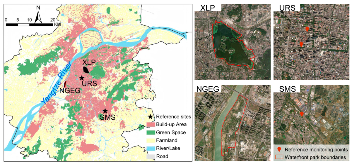
Two representative waterfront parks with mixed blue and green spaces were selected for field measurements (Figure 1,

Table 1. Characteristics of the two waterfront parks.

	Area (km2)	Perimeter (km)	Water Area (%)	Green Area (%)	Impervious (%)	Altitude (m)	Characteristics
NGEG	1.6	5.13	3	70	27	8	Near the Yangtze River
XLP	5.02	10.87	73	16	11	9	Lakeside park in the city core

). The Nanjing Green Expo Garden (NGEG) is a ribbon-shaped park along the Yangtze River and is currently the largest riverside park in Nanjing, supporting a high plant biodiversity of over 600 species. The Xuanwu Lake Park (XLP) is organized around a large urban lake (437 ha), with green spaces distributed mainly along the ring-shaped lakeside walkways and across four islands scattered within the lake.

To establish a baseline for assessing the thermal effects of the waterfront parks, two reference sites with contrasting landscape characteristics were selected (Figure 1). The urban reference site (URS) was represented by two fixed monitoring sites located in the central business district, approximately 6.8 km from NGEG and 2.8 km from XLP. One site was located along a tree-lined arterial road, whereas the other was located along an urban local road without adjacent vegetation. Both sites were equipped with the same temperature sensors and followed the same installation and logging protocol as the monitoring sites within the parks. Their synchronized hourly air temperatures were averaged to generate the URS temperature series. The suburban meteorological site (SMS) was a national-standard surface meteorological station located at the urban fringe, approximately 21 km from NGEG and 18 km from XLP. Its surroundings consisted mainly of shrubs, with sparsely distributed low-rise industrial and residential land. Hourly meteorological observations were obtained from the National Meteorological Science Data Center of the China Meteorological Administration [50].

2.2. Field Measurement

Thermal studies in urban areas commonly employ remote sensing, numerical modeling, mobile surveys, and fixed-station observations. Remote sensing offers spatially continuous LST data but has low temporal resolution, and LST is less indicative of thermal comfort than air temperature. Numerical models enable scenario testing but require site-specific calibration and are sensitive to input uncertainties. Mobile surveys provide wide coverage across diverse locations but need temporal corrections and typically have lower accuracy. Fixed-station air temperature monitoring, by contrast, delivers accurate, continuous, long-term records, making it well suited for capturing diurnal dynamics and land cover contrasts. However, establishing a dense monitoring network is demanding in terms of instrumentation, labor, and site access. Given our focus on diurnal temperature variations and configuration-level comparisons, we adopted a fixed-station design with hourly air temperature logging at the two waterfront parks.

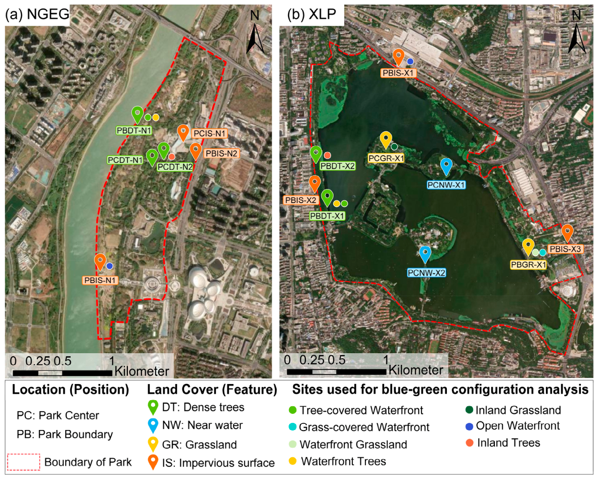
A total of 15 fixed monitoring sites were established across the two parks, with 6 in NGEG and 9 in XLP. The sites were selected according to geographic location, land cover characteristics, and installation feasibility, and were distributed between the park centers (PC) and boundaries (PB). Four land cover types were represented: near-water areas (NW), dense tree canopies (DT), impervious surfaces (IS), and grasslands (GR). Fourteen sites were initially established in August 2020. Because the monitoring sensor at PBDT-N1 was lost during the observation period, complete 2020 records were available from 13 sites, including 5 in NGEG and 8 in XLP. On 24 September 2020, a replacement sensor was installed at PBDT-N1 and an additional site, PBDT-X2, was established, bringing the final network to 15 sites (Figure 2).

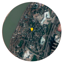
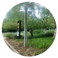
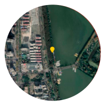
The satellite images, low-altitude photographs, and properties of the 15 sites are listed in

Table 2. Details of the 15 sites, including satellite images, low-altitude images, and features.

Satellite Image (Radius 500 m)	Low-Altitude Photograph	Properties	Satellite Image (Radius 500 m)	Low-Altitude Photograph	Properties
		PCDT-N1 LAI = 1.22 SVF = 0.22 D = 274 PC, DT			PCDT-N2 LAI = 1.08 SVF = 0.24 D = 326 PC, DT
		PCIS-N1 LAI = 0.02 SVF = 0.73 D = 326 PC, IS			PCGR-X1 LAI = 0.35 SVF = 0.52 D = 119 PC, GR
		PCNW-X1 LAI = 0.69 SVF = 0.42 D = 26 PC, NW			PCNW-X2 LAI = 1.20 SVF = 0.18 D = 4 PC, NW
		PBIS-N1 LAI = 0.00 SVF = 1.00 D = 46 PB, IS, NW			PBIS-N2 LAI = 0.64 SVF = 0.50 D = 540 PB, IS
		PBIS-X1 LAI = 0.01 SVF = 0.86 D = 17 PB, IS, NW			PBIS-X2 LAI = 0.22 SVF = 0.58 D = 99 PB, IS
		PBIS-X3 LAI = 0.94 SVF = 0.29 D = 379 PB, IS			PBDT-X1 LAI = 1.25 SVF = 0.21 D = 20 PB, DT, NW
		PBGR-X1 LAI = 0.46 SVF = 0.77 D = 11 PB, GR, NW			PBDT-N1 LAI = 1.80 SVF = 0.18 D = 20 PB, DT, NW
		PBDT-X2 LAI = 1.95 SVF = 0.11 D = 100 PB, DT

Notes: Park center = PC, park boundary = PB, near water = NW, impervious surface = IS, dense trees = DT, grasses = GR, distance from water (m) = D, leaf area index = LAI, sky view factor = SVF.

. All park sites and the two URS monitoring points were equipped with factory-calibrated HOBO MX2301 Temp/RH data loggers (Onset Computer Corporation, Bourne, MA, USA), each housed in a matching naturally ventilated solar radiation shield. The stated accuracies were ±0.2 °C for air temperature over 0–70 °C (resolution: 0.02 °C). Prior to deployment, all loggers were intercompared in an open outdoor setting on campus over 24 h and showed temperature differences within ±0.2 °C. To ensure instrument safety, the shielded loggers were mounted approximately 2.5 m above ground, below the lamp heads, with the sensing elements isolated from the supporting poles to minimize potential radiative and conductive heat interference. A previous field comparison using the same monitoring setup showed temperature differences of 0.1–0.2 °C between fixed sensors at 2.5 m and mobile sensors at 1.5 m [23]. Yang and Zhao [54] further reported that, regardless of land cover type, air temperature varied markedly with height near the ground but became relatively stable above 0.8 m. Data were recorded hourly and downloaded in situ via Bluetooth. During a supplementary field survey in September 2021, LAI and SVF were measured at the same monitoring sites using a HemiView Canopy Analysis System (Delta-T Devices Ltd., Cambridge, UK), comprising a Canon EOS 50D camera, a Sigma EX DC 4.5 mm fisheye lens, and HemiView 2.1 SR4 software. The fisheye photographs were processed in HemiView to derive LAI and SVF. The survey was conducted in the same late-summer period as the September 2020 temperature case day to reduce seasonal phenological differences, and the resulting values were used as approximate descriptors of canopy structure and sky exposure.

2.3. Data Analysis

To distinguish the overall, spatial, and configurational thermal effects of waterfront parks, the analysis considered three complementary aspects: reference–site contrasts, spatial variations among locations and land cover types, and differences among blue–green configurations. Daytime and nighttime periods were analyzed separately to account for their distinct thermal processes.

Air temperature (T_a) data were continuously recorded from 20 August 2020 to 31 August 2021. To ensure temporal consistency, data collected from August 20 to 10 September 2020, when most monitoring sites had complete records, were used to analyze the overall summer thermal effects of the waterfront parks. The meteorological conditions during this period are summarized in

Table 3. The weather conditions on 22 days (20 August 2020 to 10 September 2020) according to the data from the SMS.

	Min	Max	Mean	Standard Deviation
Ta (°C)	21.3	36.2	28.1	3.3
Precipitation (mm/d)	0	15.5	1.7	3.7
Solar radiation (W m−2)	88	526	373	109
Wind speed (m/s)	0	6.9	2	1.2
RH (%)	22	100	72.8	20.8

. Early September in Nanjing still exhibits summer-like conditions, characterized by strong solar radiation and high air temperatures. Daily weather types were classified using cloud cover and precipitation observations from the SMS in accordance with the Basic Terminology of Weather Forecast [55]. Sunny and cloudy days were defined by total cloud cover < 20% and ≥20%, respectively, while any day with daily precipitation ≥0.1 mm was classified as rainy, overriding the cloud-cover-based classification. The same weather classification criteria were applied to the corresponding 2021 analysis period.

Three sets of analyses were conducted. First, to examine the temporal patterns of park thermal effects, hourly air temperature differences (ΔT) between the waterfront parks and reference sites were calculated over the study period and under different weather conditions. A negative ΔT indicates cooling, whereas a positive ΔT indicates warming.

Second, spatial patterns were examined by comparing monitoring sites classified by location—park center (PC) or park boundary (PB)—and land cover type—dense trees (DT), near water (NW), impervious surfaces (IS), or grassland (GR). Sunny days were identified using the predefined weather classification criteria and background meteorological records, and were retained only when complete observations were available for the corresponding analyses. All ten qualifying days in each dataset were included; the specific dates are listed in

Table A1. Sunny days included in the spatial and blue–green configuration analyses.

Dataset	Analysis	Included Sunny Dates	Days (n)
2020	Location and land cover comparisons	22, 24, and 28 August; 3–9 September 2020	10
2021	Blue–green configuration comparisons	19, 21, 22, and 31 July; 1, 2, 6, 7, 10, and 16 August 2021	10

. Data from 3 September 2020 were used only to illustrate diurnal variations among park locations and land cover types, while data from 1 August 2021 were used only to illustrate diurnal variations among blue–green configurations. The blue–green analysis compared tree-covered waterfronts with open waterfronts, waterfronts with inland trees, waterfronts with inland grassland, and grass-covered waterfronts with open waterfronts.

Third, land cover data were obtained by visually interpreting 2020 Google Earth imagery into blue, green, and gray spaces at a 10 m resolution. Stratified random validation yielded an overall accuracy of 96% and a Kappa coefficient of 0.72. Buffers of 10–500 m were generated in ArcGIS Desktop 10.8 to calculate the proportions of blue (BLUS), gray (GRAS), and green space (GRES). Pearson correlations and linear regressions were performed in IBM SPSS Statistics 27.0 using daytime and nighttime mean ΔT values from 3 September 2020 (n = 13). Regressions were fitted only for relationships that remained significant after FDR correction.

To avoid pseudoreplication, hourly data were aggregated into site-by-date 24 h, daytime, and nighttime means, as appropriate. PC–PB differences were tested across the ten sunny days using linear mixed-effects models, with location as a fixed effect and site and date as random intercepts; the four park-by-period tests formed one FDR family. Land cover differences were evaluated from ten-day site means using a linear model with land cover type as the main factor and park as an adjustment factor, followed by an overall F test and pairwise comparisons. The two overall tests formed one FDR family, and the 12 pairwise comparisons formed a separate FDR family. Inter-park differences between NGEG and XLP were tested using paired t tests based on date-matched means from the 22-day monitoring period; the three period-specific tests formed one FDR family. Blue–green configuration pairs were compared using paired-sample t tests across ten sunny days, with all 18 configuration-by-period tests treated as one FDR family. Benjamini–Hochberg correction was applied throughout, and 95% confidence intervals were reported.

3. Results

3.1. Temporal Pattern of Thermal Effects

3.1.1. Overall Thermal Effects

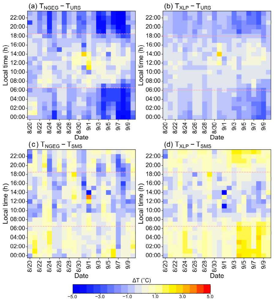
Figure 3 depicts the hourly ΔT between the waterfront parks and the URS and SMS. The T_a of each park was averaged across all monitoring sites within it. When compared with URS, both parks exhibited a dominant cooling effect throughout the monitoring period. NGEG experienced cooling for 478 of the 528 total hours (90.5%), with a maximum cooling intensity of 4.9 °C. Warming occurred during only 50 h (9.5%), with a maximum intensity of 2.7 °C. XLP showed a longer cooling duration but weaker intensity: 503 h (95.3%) with a maximum cooling of 3.0 °C, while the remaining 25 h exhibited warming (maximum 2.9 °C) or near-equal temperatures.

When SMS was used as the reference, warming was more frequent than in the URS-based comparison and dominated in XLP. Warming occurred during 255 h (48.3%) in NGEG and 354 h (67.0%) in XLP.

The diurnal patterns also differed markedly by reference site. Relative to URS, the parks were cooler at night (19:00–06:00 the following day) and warmer during the day (08:00–14:00). In contrast, relative to SMS, they showed daytime cooling (07:00–18:00) and nighttime warming. These contrasting patterns reflect differences in thermal properties and energy balance between vegetation, water, and paved surfaces. The parks warmed and cooled more slowly than SMS because of water’s high heat capacity, resulting in lower daytime and higher nighttime temperatures. This is consistent with previous LCZ studies in Nanjing, which reported daytime cooling and nocturnal warming in water bodies relative to low-plant-level areas [52]. In contrast, the compact urban form of URS blocks solar radiation during the day but traps long-wave radiation at night, making the parks warmer than URS during the daytime but cooler at night. Therefore, these patterns should be interpreted as reference-dependent thermal contrasts.

A comparison of the two parks showed that NGEG had stronger mean cooling (1.5 °C and 0.8 °C relative to URS and SMS, respectively) than XLP (0.9 °C and 0.6 °C). Mean warming intensities for NGEG were 0.4 °C and 0.6 °C relative to URS and SMS, compared with 0.3 °C and 0.8 °C for XLP. The corresponding date-level park–reference contrasts are summarized in

Table 4. Park–reference air temperature contrasts by park, reference site, and period.

Park	Reference	Period	n	Mean ΔT (°C)	95% CI	Raw p	pFDR
NGEG	SMS	24 h	22	−0.119	[−0.321, 0.083]	0.234	0.255
		Daytime	22	−0.309 *	[−0.530, −0.087]	0.009	0.011
		Nighttime	21	0.055	[−0.191, 0.301]	0.647	0.647
	URS	24 h	22	−1.207 **	[−1.487, −0.928]	<0.001	<0.001
		Daytime	22	−0.512 **	[−0.667, −0.357]	<0.001	<0.001
		Nighttime	21	−1.968 **	[−2.527, −1.410]	<0.001	<0.001
XLP	SMS	24 h	22	0.345 **	[0.180, 0.511]	<0.001	<0.001
		Daytime	22	−0.157	[−0.324, 0.010]	0.063	0.076
		Nighttime	21	0.868 **	[0.620, 1.116]	<0.001	<0.001
	URS	24 h	22	−0.743 **	[−0.861, −0.626]	<0.001	<0.001
		Daytime	22	−0.360 **	[−0.448, −0.273]	<0.001	<0.001
		Nighttime	21	−1.155 **	[−1.403, −0.907]	<0.001	<0.001

Note: ΔT = Tpark − Treference; negative values indicate cooler park conditions relative to the reference. Raw p-values are unadjusted, whereas p_FDR values were adjusted using the Benjamini–Hochberg procedure. * p_FDR < 0.05; ** p_FDR < 0.01.

. Using date-level means, NGEG was 0.5 °C cooler than XLP over 24 h and 0.8 °C cooler at night (both p_FDR < 0.001), whereas the daytime difference was not statistically supported (p_FDR = 0.056;

Table 5. Date-level paired air temperature differences between NGEG and XLP by period.

Period	n Pairs	NGEG–XLP Difference (°C)	95% CI	Raw p	pFDR
24 h	22	−0.464 **	[−0.649, −0.279]	<0.001	<0.001
Daytime	22	−0.152	[−0.307, 0.004]	0.056	0.056
Nighttime	21	−0.813 **	[−1.148, −0.478]	<0.001	<0.001

Note: ** p_FDR < 0.01.

). These differences may partly reflect NGEG’s higher vegetation cover and greater distance from the city center, which may reduce warm air advection from surrounding built-up areas. Overall, these findings highlight the potential importance of vegetation around water bodies for improving the cooling performance of waterfront parks.

3.1.2. Thermal Effects Under Different Weather Scenarios

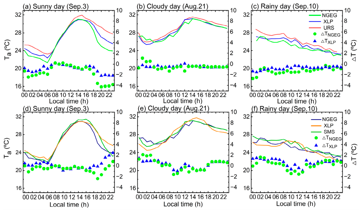
Figure 4a–c present the diurnal profiles of T_a and ΔT on representative sunny, cloudy, and rainy days. On sunny days, both T_a and ΔT exhibited greater diurnal fluctuations than on cloudy or rainy days. At midnight (00:00), the parks were cooler than URS by approximately 1.3 °C (NGEG) and 0.8 °C (XLP), with this cooling persisting until 08:00. Between 08:00 and 12:00, park temperatures were comparable to URS. From 12:00 onward, park T_a began to drop below URS, reaching the maximum cooling at 20:00, with reductions of 4.3 °C (NGEG) and 2.1 °C (XLP). Under cloudy and rainy conditions, only marginal cooling or warming was observed, with ΔT remaining near zero throughout the day. Figure 4d–f show the corresponding comparisons using the SMS as the reference. Again, sunny days produced the largest ΔT amplitudes (−2.4 to 2.5 °C), compared with cloudy (−1.6 to 2.1 °C) and rainy (−1.4 to 1.6 °C) days. Across all weather types, a consistent diurnal pattern emerged: cooling during the daytime (07:00–18:00) and slight warming at night (19:00–06:00 the following day). NGEG extended its cooling effect until 22:00, likely due to its greater vegetation cover enhancing nocturnal cooling. The maximum cooling (warming) intensities were 2.4 °C (0.8 °C) for NGEG and 0.9 °C (2.5 °C) for XLP, both observed on sunny days.

Because the park–reference temperature contrasts were greatest under sunny conditions, the subsequent comparisons focused on sunny days. Representative sunny days were used only to illustrate diurnal patterns, whereas statistical inference was based on all sunny days with complete observations.

3.2. Spatial Pattern of Thermal Effects

3.2.1. Variations Between Different Locations

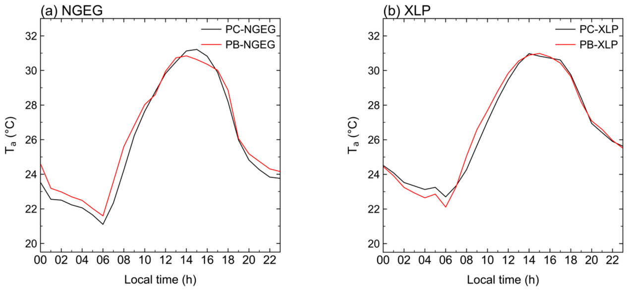
Figure 5 illustrates the diurnal variations in T_a between PC and PB sites on the representative sunny day of 3 September 2020 (n = 13). In NGEG, PC sites were cooler than PB sites from midnight to late morning (0.4–1.7 °C), but this difference diminished at around noon (−0.1 to 0.3 °C) and even reversed in the afternoon, when PC became up to 0.6 °C warmer than PB. After 17:00, PC regained a slight cooling advantage (0.1–0.7 °C), albeit weaker than in the morning. In XLP, PB was cooler than PC during the early morning (0.1–0.6 °C), while PC became cooler between 08:00 and 13:00 (0.4–0.9 °C); temperatures at PC and PB remained similar for the rest of the day.

Overall, PC sites did not consistently remain cooler than PB sites throughout the day. Linear mixed-effects models based on the ten sunny days estimated PC–PB differences of −0.3 °C during daytime and −0.5 °C at night in NGEG, and −0.4 and −0.1 °C, respectively, in XLP. None of these differences were significant after FDR correction (all p_FDR ≥ 0.383; all 95% CIs included zero;

Table 6. Estimated PC–PB air temperature differences across ten sunny days.

Park	Period	Sites (n)	Dates (n)	Estimated Difference (°C)	95% CI	Raw p	pFDR
NGEG	Daytime	5	10	−0.307	[−1.599, 0.985]	0.642	0.753
	Nighttime	5	10	−0.505	[−1.979, 0.969]	0.502	0.753
XLP	Daytime	8	10	−0.368	[−0.814, 0.078]	0.096	0.383
	Nighttime	8	10	−0.092	[−0.666, 0.482]	0.753	0.753

Note: Differences were calculated as PC−PB; negative values indicate cooler PC sites.

).

3.2.2. Variations Between Different Land Cover Features

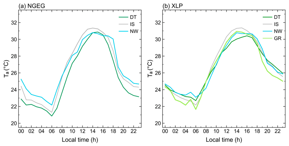
Figure 6 illustrates the diurnal variations in T_a across DT, NW, GR, and IS on the representative sunny day of 3 September 2020. In both parks, IS generally exhibited higher daytime temperatures than the other land cover types. In NGEG, DT remained cooler than IS throughout the day, with a maximum temperature difference of approximately 1.9 °C occurring between 14:00 and 15:00. In XLP, DT was cooler than IS mainly between 09:00 and 19:00, with a maximum difference of approximately 1.4 °C at 12:00. NW sites generally showed lower temperatures during the day and higher temperatures at night. The maximum daytime IS–NW difference was approximately 1.0 °C in both parks, while the maximum nighttime warming of NW relative to IS reached approximately 1.4 °C in NGEG and 1.1 °C in XLP. In XLP, the GR profile was broadly comparable to that of NW, with a maximum nighttime reduction of approximately 1.1 °C relative to IS.

Based on the ten sunny days, the park-adjusted linear model showed a statistically supported overall daytime difference among land cover types (F(3, 8) = 13.04, p_FDR = 0.004). Among the pairwise comparisons, only IS and DT remained significantly different after FDR correction, with IS being 1.0 °C warmer than DT (95% CI: 0.6–1.4 °C, p_FDR = 0.004;

Table 7. Park-adjusted pairwise comparisons among land cover types across ten sunny days.

Period	Contrast	Mean Difference (°C)	95% CI	Raw p	pFDR
Daytime	IS−DT	1.042 **	[0.644, 1.441]	<0.001	0.004
	IS−NW	0.577	[0.188, 0.966]	0.009	0.055
	IS−GR	0.536	[0.071, 1.001]	0.029	0.109
	DT−NW	−0.466	[−0.914, −0.017]	0.043	0.109
	DT−GR	−0.506	[−1.040, −0.028]	0.060	0.109
	NW−GR	−0.041	[−0.539, 0.458]	0.856	0.856
Nighttime	IS−DT	0.647	[−0.120, 1.413]	0.088	0.127
	IS−NW	−0.160	[−0.908, 0.589]	0.636	0.763
	IS−GR	0.734	[−0.160, 1.628]	0.095	0.127
	DT−NW	−0.806	[−1.669, −0.056]	0.063	0.109
	DT−GR	0.087	[−0.941, 1.115]	0.850	0.856
	NW−GR	0.893	[−0.065, 1.852]	0.064	0.109

Note: Differences were calculated as the first land cover type minus the second; positive values indicate that the first type was warmer. ** p_FDR < 0.01.

). The nighttime analysis did not show clear statistical evidence of an overall land cover difference (F(3, 8) = 2.96, p_FDR = 0.098;

Table 8. Park-adjusted overall differences among land cover types across ten sunny days.

Period	F (df1, df2)	Raw p	pFDR
Daytime	13.04 ** (3, 8)	0.002	0.004
Nighttime	2.96 (3, 8)	0.098	0.098

Note: ** p_FDR < 0.01.

).

3.2.3. Integrated Cooling Effects of Blue–Green Spaces

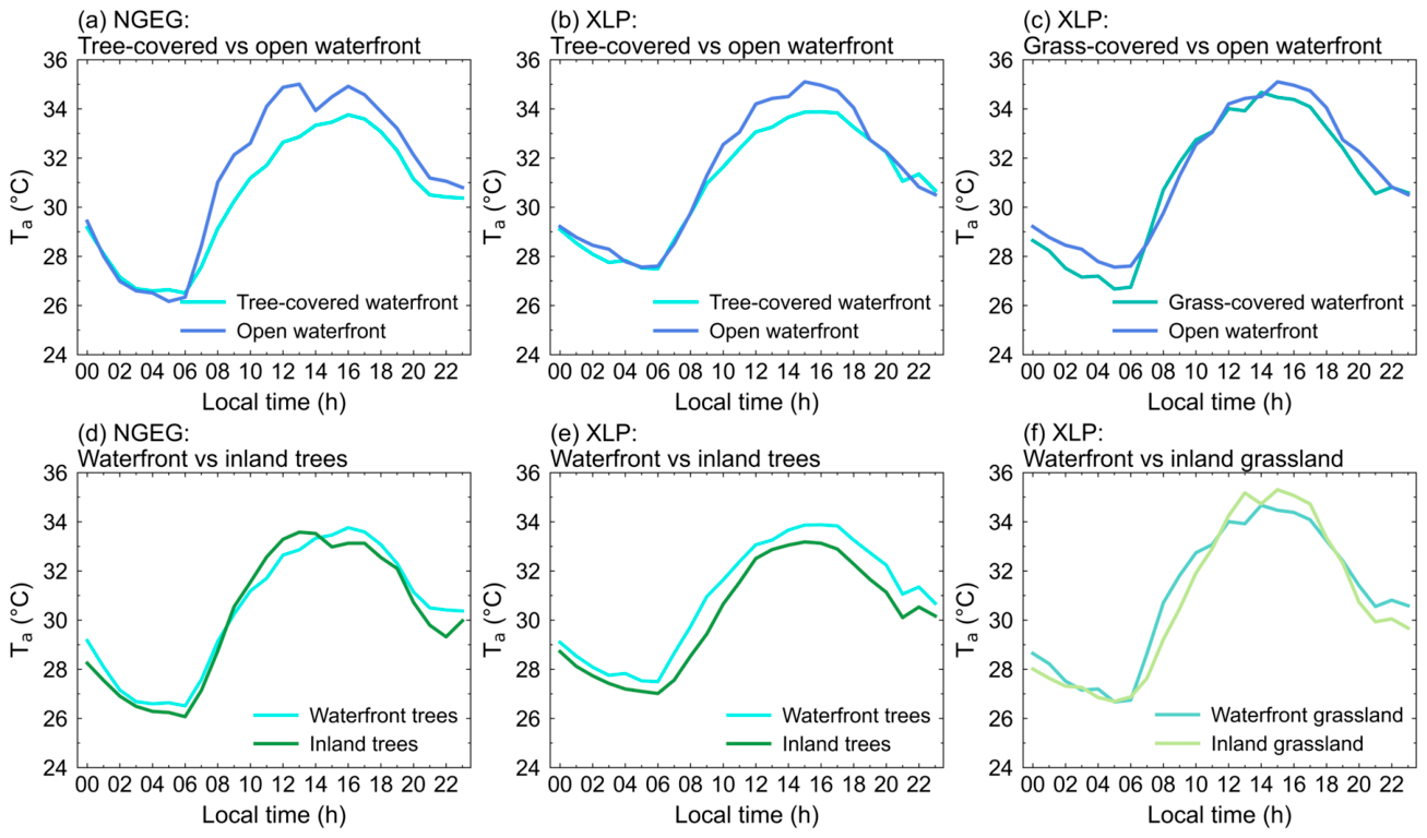
Figure 7 presents the diurnal T_a variations across different blue–green configurations in the two waterfront parks on the representative sunny day (1 August 2021). Overall, the tree-covered waterfront and grass-covered waterfront configurations were generally cooler than the open waterfront configuration. The tree-covered waterfront was cooler than the open waterfront during most daytime hours, with 24 h mean temperature reductions of 0.8 °C in NGEG and 0.4 °C in XLP. The maximum reductions, reaching 2.4 °C and 1.2 °C, respectively, occurred during daytime, consistent with the canopy shading effect. In contrast, the grass-covered waterfront was cooler than the open waterfront mainly at night, with a maximum difference of 1.1 °C, possibly associated with nocturnal radiative cooling and residual evapotranspiration.

The potential influence of water proximity on vegetation cooling was further examined by comparing waterfront trees with inland trees and waterfront grassland with inland grassland. On the representative day, waterfront trees were slightly warmer than inland trees in NGEG and remained warmer throughout the day in XLP. Waterfront grassland in XLP showed a narrower diurnal temperature range than inland grassland, being cooler during parts of the afternoon but warmer on average at night.

Paired-sample t tests across the ten sunny days showed that, in XLP, the tree-covered waterfront was significantly cooler than the open waterfront by 0.5 °C over 24 h, 0.8 °C during daytime, and 0.2 °C at night (all p_FDR ≤ 0.003,

Table 9. Date-level paired air temperature differences among blue–green configurations across ten sunny days.

Park	Comparison	Period	Pairs (n)	Mean ΔT (°C)	95% CI	Raw p	pFDR
NGEG	Tree-covered waterfront–open waterfront	24 h	10	0.337	[−0.224, 0.897]	0.207	0.287
		Daytime	10	−0.077	[−0.653, 0.499]	0.769	0.815
		Nighttime	10	0.750 *	[0.114, 1.386]	0.026	0.046
	Waterfront trees–inland trees	24 h	10	0.013	[−0.567, 0.594]	0.960	0.960
		Daytime	10	−0.280	[−0.853, 0.292]	0.297	0.371
		Nighttime	10	0.307	[−0.337, 0.950]	0.309	0.371
XLP	Tree-covered waterfront–open waterfront	24 h	10	−0.532 **	[−0.616, −0.448]	<0.001	<0.001
		Daytime	10	−0.840 **	[−0.940, −0.739]	<0.001	<0.001
		Nighttime	10	−0.224 **	[−0.338, −0.110]	0.002	0.003
	Waterfront trees–inland trees	24 h	10	0.466 **	[0.326, 0.606]	<0.001	<0.001
		Daytime	10	0.564 **	[0.366, 0.761]	<0.001	<0.001
		Nighttime	10	0.368 **	[0.273, 0.463]	<0.001	<0.001
	Waterfront grassland–inland grassland	24 h	10	0.028	[−0.101, 0.158]	0.634	0.713
		Daytime	10	−0.124	[−0.246, −0.003]	0.046	0.076
		Nighttime	10	0.180	[−0.020, 0.381]	0.072	0.108
	Grass-covered waterfront–open waterfront	24 h	10	−0.441 **	[−0.499, −0.383]	<0.001	<0.001
		Daytime	10	−0.239 **	[−0.314, −0.163]	<0.001	<0.001
		Nighttime	10	−0.644 **	[−0.766, −0.523]	<0.001	<0.001

Note: Differences were calculated as the first configuration minus the second; negative values indicate that the first configuration was cooler. * p_FDR < 0.05; ** p_FDR < 0.01.

). The grass-covered waterfront was also significantly cooler than the open waterfront by 0.4, 0.2, and 0.6 °C, respectively (all p_FDR < 0.001). However, waterfront trees were significantly warmer than inland trees by 0.5, 0.6, and 0.4 °C, respectively (all p_FDR < 0.001), while no significant difference was detected between waterfront and inland grassland.

In NGEG, no significant waterfront–inland tree difference was detected. The tree-covered waterfront was 0.8 °C warmer than the open waterfront at night (p_FDR = 0.046), whereas the daytime and 24 h differences were not significant.

3.3. Associations Between ΔT and Spatial Factors

The preceding analyses showed noticeable spatial variation in thermal effects across the monitoring sites, as represented by ΔT relative to the urban reference site (URS). This section examines the spatial factors associated with this variation. Relationships with immediate spatial factors (LAI and SVF) are examined first, followed by associations with the proportions of gray, blue, and green spaces at multiple buffer scales.

3.3.1. Associations Between ΔT and Immediate Spatial Factors

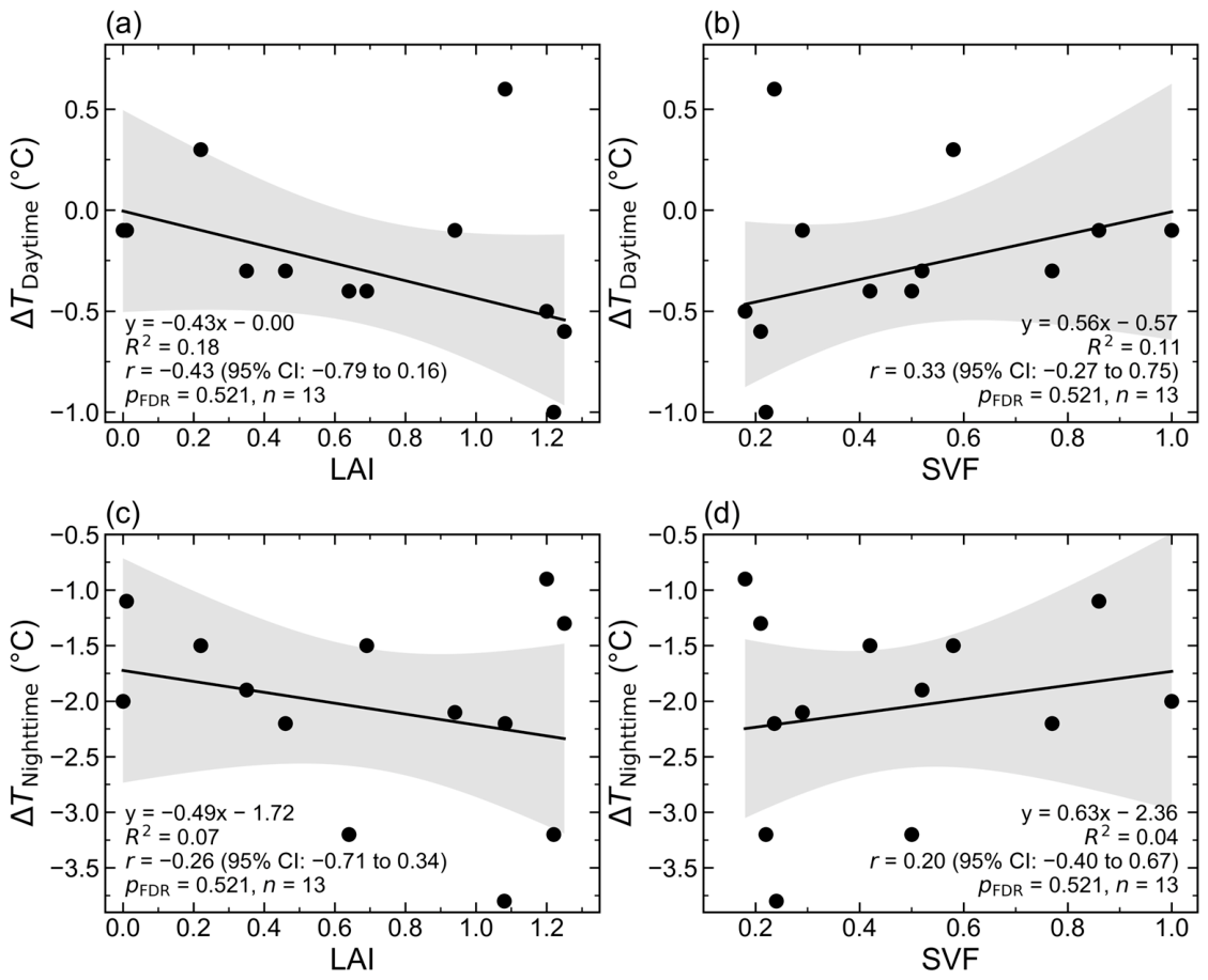
Figure 8 shows the correlations of LAI and SVF with site-level mean ΔT during daytime (07:00–18:00) and nighttime (19:00–06:00 the following day) on the representative sunny day (3 September 2020; n = 13). After Benjamini–Hochberg FDR correction across the four tests, none of the correlations remained significant (all p_FDR = 0.521), and all 95% confidence intervals included zero. Although LAI showed a negative relationship with daytime ΔT, the expected effects of canopy shading and evapotranspiration were not statistically supported. The weak relationships may partly reflect air advection and the influence of surrounding land cover beyond the immediate monitoring location. Therefore, correlations between ΔT and land cover composition were further examined at multiple scales.

3.3.2. Associations Between ΔT and Multi-Scale Land Cover Composition

Table 10. Pearson correlation coefficients between daytime and nighttime ΔT and the proportion of blue, gray, and green spaces.

Buffer Radius (m)	Daytime			Nighttime
	GRAS	BLUS	GRES	GRAS	BLUS	GRES
10 m	0.403	−0.111	−0.403	0.388	0.361	−0.396
25 m	0.715 *	−0.164	−0.676	−0.048	0.276	−0.022
50 m	0.774 *	−0.169	−0.603	−0.009	0.339	−0.224
75 m	0.753 *	−0.141	−0.572	−0.041	0.396	−0.288
100 m	0.767 *	−0.124	−0.571	−0.006	0.451	−0.400
150 m	0.810 **	−0.077	−0.574	0.063	0.541	−0.605
200 m	0.730 *	−0.028	−0.521	0.088	0.622	−0.748 *
250 m	0.591	0.001	−0.471	0.043	0.689	−0.827 **
300 m	0.452	0.000	−0.375	0.000	0.678	−0.853 **
350 m	0.381	−0.015	−0.309	−0.015	0.654	−0.866 **
400 m	0.369	−0.040	−0.271	−0.016	0.629	−0.868 **
450 m	0.360	−0.075	−0.228	−0.032	0.594	−0.846 **
500 m	0.344	−0.091	−0.207	−0.046	0.565	−0.834 **

Note: Asterisks indicate significance based on Benjamini–Hochberg FDR-adjusted p-values: * p_FDR < 0.05; ** p_FDR < 0.01. All 78 correlations were treated as a single family.

shows the correlations between land cover composition at multiple scales and site-level mean ΔT during daytime (07:00–18:00) and nighttime (19:00–06:00 the following day) on a representative sunny day (3 September 2020; n = 13). Land cover composition was expressed as the area proportions of blue, gray, and green spaces, abbreviated as BLUS, GRAS, and GRES, respectively. After Benjamini–Hochberg FDR correction across all 78 tests, daytime ΔT was positively correlated with GRAS at 25–200 m (r = 0.715–0.810, p_FDR = 0.009–0.036), but not with BLUS or GRES. At night, ΔT was negatively correlated with GRES at 200–500 m (r = −0.868 to −0.748, p_FDR = 0.005–0.023), whereas GRAS and BLUS showed no significant correlations. Full correlation statistics, including 95% confidence intervals and FDR-adjusted p-values, are provided in

Table A2. Pearson correlations between land cover proportions and ΔT across buffer radii.

Buffer Radius (m)	Variable	Daytime				Nighttime
		r	Raw p	pFDR	95% CI	r	Raw p	pFDR	95% CI
10	GRAS	0.403	0.172	0.380	[−0.190, 0.781]	0.388	0.190	0.390	[−0.207, 0.774]
	GRES	−0.403	0.173	0.380	[−0.781, 0.190]	−0.396	0.180	0.380	[−0.778, 0.198]
	BLUS	−0.111	0.717	0.982	[−0.624, 0.468]	0.361	0.226	0.411	[−0.237, 0.761]
25	GRAS	0.715 *	0.006	0.036	[0.271, 0.908]	−0.048	0.876	0.999	[−0.584, 0.516]
	GRES	−0.676	0.011	0.054	[−0.894, −0.200]	−0.022	0.943	0.999	[−0.566, 0.535]
	BLUS	−0.164	0.593	0.857	[−0.656, 0.426]	0.276	0.361	0.587	[−0.324, 0.718]
50	GRAS	0.774 *	0.002	0.018	[0.389, 0.929]	−0.009	0.976	0.999	[−0.557, 0.545]
	GRES	−0.603	0.029	0.108	[−0.866, −0.078]	−0.224	0.462	0.707	[−0.690, 0.373]
	BLUS	−0.169	0.581	0.855	[−0.659, 0.421]	0.339	0.258	0.447	[−0.261, 0.750]
75	GRAS	0.753 *	0.003	0.023	[0.346, 0.922]	−0.041	0.893	0.999	[−0.579, 0.521]
	GRES	−0.572	0.041	0.125	[−0.854, −0.031]	−0.288	0.340	0.563	[−0.724, 0.312]
	BLUS	−0.141	0.647	0.917	[−0.642, 0.445]	0.396	0.180	0.380	[−0.198, 0.778]
100	GRAS	0.767 *	0.002	0.019	[0.375, 0.927]	−0.006	0.985	0.999	[−0.555, 0.547]
	GRES	−0.571	0.042	0.125	[−0.853, −0.028]	−0.400	0.176	0.380	[−0.779, 0.194]
	BLUS	−0.124	0.685	0.955	[−0.632, 0.458]	0.451	0.122	0.297	[−0.133, 0.803]
150	GRAS	0.810 **	<0.001	0.009	[0.468, 0.941]	0.063	0.837	0.999	[−0.505, 0.594]
	GRES	−0.574	0.040	0.125	[−0.855, −0.034]	−0.605	0.028	0.109	[−0.867, −0.081]
	BLUS	−0.077	0.804	0.999	[−0.602, 0.495]	0.541	0.056	0.156	[−0.014, 0.841]
200	GRAS	0.730 *	0.005	0.030	[0.300, 0.914]	0.088	0.776	0.999	[−0.487, 0.609]
	GRES	−0.521	0.068	0.183	[−0.833, 0.043]	−0.748 *	0.003	0.023	[−0.920, −0.336]
	BLUS	−0.028	0.928	0.999	[−0.570, 0.531]	0.622	0.023	0.095	[0.109, 0.874]
250	GRAS	0.591	0.034	0.114	[0.059, 0.861]	0.043	0.889	0.999	[−0.520, 0.581]
	GRES	−0.471	0.104	0.271	[−0.811, 0.108]	−0.827 **	<0.001	0.006	[−0.947, −0.507]
	BLUS	0.001	0.998	0.999	[−0.550, 0.552]	0.689	0.009	0.051	[0.223, 0.899]
300	GRAS	0.452	0.121	0.297	[−0.132, 0.803]	0.001	0.997	0.999	[−0.550, 0.552]
	GRES	−0.375	0.207	0.404	[−0.767, 0.222]	−0.853 **	<0.001	0.005	[−0.955, −0.569]
	BLUS	0.000	0.999	0.999	[−0.551, 0.551]	0.678	0.010	0.054	[0.202, 0.895]
350	GRAS	0.381	0.200	0.399	[−0.216, 0.770]	−0.015	0.961	0.999	[−0.561, 0.541]
	GRES	−0.309	0.305	0.517	[−0.735, 0.292]	−0.866 **	<0.001	0.005	[−0.959, −0.603]
	BLUS	−0.015	0.961	0.999	[−0.561, 0.540]	0.654	0.015	0.071	[0.160, 0.886]
400	GRAS	0.369	0.215	0.409	[−0.229, 0.764]	−0.016	0.959	0.999	[−0.562, 0.540]
	GRES	−0.271	0.340	0.588	[−0.715, 0.329]	−0.868 **	<0.001	0.005	[−0.960, −0.607]
	BLUS	−0.040	0.897	0.999	[−0.578, 0.523]	0.629	0.021	0.092	[0.119, 0.876]
450	GRAS	0.360	0.226	0.411	[−0.238, 0.760]	−0.032	0.918	0.999	[−0.573, 0.529]
	GRES	−0.228	0.455	0.707	[−0.692, 0.370]	−0.846 **	<0.001	0.005	[−0.953, −0.552]
	BLUS	−0.075	0.809	0.999	[−0.601, 0.497]	0.594	0.032	0.113	[0.064, 0.863]
500	GRAS	0.344	0.250	0.442	[−0.255, 0.752]	−0.046	0.882	0.999	[−0.582, 0.518]
	GRES	−0.207	0.497	0.745	[−0.681, 0.388]	−0.834 **	<0.001	0.006	[−0.949, −0.523]
	BLUS	−0.091	0.768	0.999	[−0.611, 0.484]	0.565	0.044	0.128	[0.021, 0.851]

Note: * p_FDR < 0.05; ** p_FDR < 0.01.

.

During daytime, solar radiation is a major source of surface heating. Unshaded impervious surfaces absorb and store solar energy and may heat the near-surface air. Therefore, the positive GRAS–ΔT relationship indicates weaker cooling at sites surrounded by more gray space, consistent with previous findings [56]. Although GRES showed negative coefficients, none remained significant after FDR correction.

At night, GRES was negatively correlated with ΔT at 200–500 m. Although canopy shading no longer operated, vegetated surfaces may store less daytime heat than impervious surfaces and continue to cool through longwave heat loss and residual evapotranspiration. The broader significant range may therefore reflect the cumulative contribution of surrounding green space to nighttime cooling.

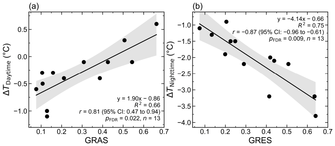
Figure 9 further illustrates the strongest daytime association between GRAS and ΔT at 150 m. Within the observed range, each additional 10% of the buffer area occupied by gray space was associated with a 0.19 °C increase in ΔT, indicating weaker daytime cooling, likely due to greater solar heat absorption and storage by impervious surfaces.

At night, the strongest association occurred between GRES and ΔT at 400 m. Within the observed range, each additional 10% of the buffer area occupied by green space was associated with a 0.41 °C decrease in ΔT, indicating stronger nighttime cooling through lower heat storage, longwave heat loss, and residual evapotranspiration. These regressions describe sample-specific associations rather than universal thresholds.

4. Discussion

4.1. Overall Thermal Performance of Waterfront Parks

Urban waterfront parks represent a unique landscape type in which blue and green spaces co-exist and interact. Particularly in cities with extensive waterway networks, design guidelines increasingly encourage the integration of blue and green spaces into a unified blue–green infrastructure system to deliver multiple ecosystem and aesthetic benefits. In this study, we compared the hourly air temperature between two waterfront parks and two reference sites that differed markedly in both location and landscape characteristics. The magnitudes and diurnal patterns of the thermal effects observed in the two parks were highly dependent on the choice of reference sites. When compared with the urban reference site in the CBD, both parks exhibited a nearly day-long cooling effect. However, when the suburban meteorological station was adopted as the reference, a pronounced nocturnal warming effect emerged in both parks. This finding is consistent with many studies reporting the cooling potential of urban water bodies [57], while also aligning with studies that have concluded that UBS may exacerbate UHI effects under specific conditions [6].

These seemingly contradictory observations can be largely attributed to the contrasting thermal regimes of two reference environments. The compact, high-density urban fabric of the CBD tends to trap heat during the night, whereas the more open and low-rise suburban area allows for more effective nocturnal radiative cooling. As a result, the thermal contrast between the parks and the reference site varies substantially depending on whether the reference is urban or suburban. This discrepancy provides a plausible explanation for the ongoing debate in the literature regarding whether, and under what circumstances, urban water bodies exert warming or cooling effects. More importantly, it underscores the importance of careful reference site selection when assessing the thermal performance of urban parks. The reported ΔT values therefore represent reference-dependent thermal contrasts and should not be attributed solely to the parks or water bodies.

The finding that a water body might augment the UHI intensity does not mean that water areas could not benefit the urban thermal environment. A large water body in an urban center can enhance air ventilation due to the open space and the creation of local circulation, thereby improving the thermal comfort of urban residents. For a holistic understanding of the influence of waterfront parks on urban climates, other parameters such as radiation, wind, and humidity should also be measured.

4.2. Effects of Location and Land Cover Type

We examined the spatial variations in air temperature within each park in relation to both the location and land cover characteristics of the measuring sites. Linear mixed-effects models based on the ten sunny days did not provide statistical support for PC–PB differences in either park during daytime or nighttime (all p_FDR ≥ 0.383; all 95% CIs included zero). By contrast, the park-adjusted linear model showed a significant overall daytime difference among land cover types (F(3, 8) = 13.04, p_FDR = 0.004). Thus, the statistical evidence for daytime land cover differences was stronger than that for center–boundary differences.

The correlation analysis further revealed scale-dependent relationships between ΔT and landscape factors. Neither the leaf area index (LAI) nor sky view factor (SVF) were significantly associated with daytime or nighttime ΔT after FDR correction, indicating potential influences of background land cover features surrounding the sites. The multi-scale analysis nevertheless showed that daytime ΔT was positively correlated with the proportion of gray space (GRAS) at 25–200 m (r = 0.715–0.810, p_FDR = 0.009–0.036), whereas nighttime ΔT was negatively correlated with the proportion of green space (GRES) at 200–500 m (r = −0.868 to −0.748, p_FDR = 0.005–0.023). No correlations involving the proportion of blue space (BLUS) remained significant.

These divergent patterns can be attributed to the distinct surface-energy processes during daytime and nighttime. Under strong incoming solar radiation, unshaded impervious surfaces absorb and store heat, providing a plausible explanation for the positive GRAS–ΔT relationship. At night, lower heat storage, continued longwave heat loss, and residual evapotranspiration from vegetation may explain the negative GRES–ΔT relationship. The 200–500 m range of the nighttime green-space associations is comparable in magnitude to the cooling distances of 391 m for parks and 469 m for forests reported by Jaganmohan et al. [21] but is smaller than the 1.4 km reported by Yan et al. [22] and overlaps the road-dependent distances of 267 and 883 m reported by Yin et al. [23].

4.3. Integrated Cooling Effect of Blue and Green Spaces

Urban vegetation and water have been widely recognized as key nature-based solutions for mitigating urban overheating. Recent studies have examined combined blue–green cooling effects, but most have treated vegetation as a single category and relied on discrete time measurements. Our study addressed these gaps by conducting continuous hourly air temperature measurements across different blue–green configurations in two waterfront parks. Specifically, we compared tree-covered waterfronts with open waterfronts, grass-covered waterfronts with open waterfronts, waterfronts with inland trees, and waterfronts with inland grasslands.

Compared with previous studies that reported either positive synergy [41] or no added cooling [42], our study demonstrates that blue–green thermal interactions can be positive, neutral, or even negative, depending on park and vegetation type and time of day. On a typical sunny summer day, the tree-covered waterfronts were cooler than the open waterfronts during most daytime hours, with 24 h mean temperature reductions of 0.8 °C in NGEG and 0.4 °C in XLP; the maximum reductions were 2.4 and 1.2 °C, respectively. The grass-covered waterfronts were cooler than the open waterfronts mainly at night, with a maximum difference of 1.1 °C. Across the ten sunny days, these cooling differences were statistically supported in XLP, whereas most NGEG comparisons were not statistically supported. Second, proximity to water did not consistently enhance vegetation cooling. In NGEG, no significant waterfront–inland tree difference was detected. In XLP, waterfront trees were even warmer than inland trees throughout the day. Conversely, waterfront–inland grassland differences were not statistically supported.

One possible explanation for the limited cooling benefit of waterfront trees is that higher humidity near water may reduce the vapor pressure deficit and evapotranspirative demand. In addition, greater openness and airflow at waterfront sites may disperse canopy-cooled air rather than allow it to accumulate locally. These mechanisms were not tested directly, and the observed differences may also reflect uncontrolled variation in tree species, canopy structure, crown size, and the surrounding built environment. Climate-sensitive designs must therefore consider vegetation type, diurnal timing, and local micro-environmental conditions jointly.

4.4. Implications for the Climate-Sensitive Design of Waterfront Parks

Our findings offer several practical implications for the climate-sensitive design of waterfront planning in subtropical cities. First, the significant daytime difference between dense tree sites and impervious surface sites supports prioritizing shaded vegetation and reducing extensive unshaded impervious surfaces. Second, open water bodies should be integrated with vegetation to create a more favorable microclimate. Vegetated waterfront corridors can also support stormwater management, biodiversity, and water purification. This co-benefits approach can connect urban heat mitigation with sponge-city implementation through integrated blue–green infrastructure and coordinated planning [58]. Among vegetation types, trees provide substantially stronger cooling than grasses due to their shading capacity and sustained evapotranspiration. Third, the design of landscape nodes in waterfront parks should consider the surrounding blue–green–gray compositions within appropriate spatial scales. The scale-dependent associations (gray space at 25–200 m daytime; green space at 200–500 m nighttime) and their estimated magnitudes (+0.19 °C per 10% gray space; −0.41 °C per 10% green space) can serve as candidate screening ranges for municipal waterfront and greenway plans. Local validation through municipal pilot projects, long-term monitoring, and interdepartmental coordination are needed to translate these site-specific findings into locally calibrated climate action targets. More broadly, garden city and sustainable park strategies should combine ecological resilience with accessibility, public participation, and adaptation to local environmental and cultural conditions [59].

4.5. Limitations of This Study

This study has several limitations that should be acknowledged when interpreting its findings and applying them to practice. First, the monitoring network comprised 15 sites across only two parks within a single subtropical city, which limits statistical power and generalizability to other climatic or urban contexts. Expanding the network to include more parks and spatial replicates would enable more robust inference and help validate the aforementioned planning implications before they are incorporated into local design guidelines. Second, although we distinguished between trees and grasses, the range of vegetation types was limited; future studies might include shrubs, mixed woodlands, and other plant communities to identify which vegetation characteristics most strongly modulate the thermal interactions between blue and green spaces. Third, the measured air temperature is insufficient to represent pedestrian thermal comfort. In waterfront environments, wind speed, solar radiation, and humidity strongly influence heat stress, and the enhanced ventilation typical of open waterfronts may substantially affect perceived thermal conditions. Future research might include these variables and adopt multi-parameter indices such as PET or UTCI to better capture human thermal comfort in waterfront areas.

5. Conclusions

This study examined air temperature patterns in two waterfront parks in subtropical Nanjing using measurements from a network of 15 park sites together with urban and suburban reference data. It assessed park–reference temperature contrasts, differences among land cover types, multi-scale land cover associations, and the thermal performance of selected blue–green configurations. The focus of the study was to investigate the integrated effect of blue and green spaces with reference to different vegetation types and diurnal periods.

Both parks exhibited cooling and warming depending on the time of day and reference environment. Daytime and nighttime temperatures were associated with gray- and green-space proportions, respectively, at distinct buffer scales, with blue-space proportions showing no significant correlation with air temperatures. The vegetation-covered waterfronts were cooler than the open waterfronts in XLP, but the waterfront vegetation had higher air temperatures than their inland counterparts. The results suggested that the integrated effect of blue and green spaces is highly context-dependent, varying with vegetation type and diurnal period.

Future studies can strengthen spatial and temporal replication, include a broader spectrum of vegetation forms, and incorporate measurements of humidity, wind speed, and radiant conditions to enable more comprehensive assessments of pedestrian thermal comfort under different blue–green configurations.

References

1. Cheval, S.; Amihăesei, V.-A.; Chitu, Z.; Dumitrescu, A.; Falcescu, V.; Irașoc, A.; Micu, D.M.; Mihulet, E.; Ontel, I.; Paraschiv, M.-G.; et al. A Systematic Review of Urban Heat Island and Heat Waves Research (1991–2022). Clim. Risk Manag. 2024, 44, 100603. [Google Scholar] [CrossRef] [Scilit]
2. Yadav, N.; Rajendra, K.; Awasthi, A.; Singh, C.; Bhushan, B. Systematic Exploration of Heat Wave Impact on Mortality and Urban Heat Island: A Review from 2000 to 2022. Urban Clim. 2023, 51, 101622. [Google Scholar] [CrossRef] [Scilit]
3. Zhang, X.; Li, Q.; Wang, B.; Qian, X.; Liu, W.; Guo, Y.; Wu, Z.; Cao, Z.; Qin, C.; Zhai, J.; et al. A Comprehensive Review of Blue, Green, and Grey Space Studies for Improving Urban Microclimate. Build. Environ. 2026, 300, 114698. [Google Scholar] [CrossRef] [Scilit]
4. Budzik, G.; Sylla, M.; Kowalczyk, T. Understanding Urban Cooling of Blue–Green Infrastructure: A Review of Spatial Data and Sustainable Planning Optimization Methods for Mitigating Urban Heat Islands. Sustainability 2025, 17, 142. [Google Scholar] [CrossRef] [Scilit]
5. Yu, Z.; Yang, G.; Zuo, S.; Jørgensen, G.; Koga, M.; Vejre, H. Critical Review on the Cooling Effect of Urban Blue-Green Space: A Threshold-Size Perspective. Urban For. Urban Green. 2020, 49, 126630. [Google Scholar] [CrossRef] [Scilit]
6. Fricke, L.; Legg, R.; Kabisch, N. Impact of Blue Spaces on the Urban Microclimate in Different Climate Zones, Daytimes and Seasons—A Systematic Review. Urban For. Urban Green. 2024, 101, 128528. [Google Scholar] [CrossRef] [Scilit]
7. Galalizadeh, S.; Morrison-Saunders, A.; Horwitz, P.; Silberstein, R.; Blake, D. The Cooling Impact of Urban Greening: A Systematic Review of Methodologies and Data Sources. Urban For. Urban Green. 2024, 95, 128157. [Google Scholar] [CrossRef] [Scilit]
8. Ampatzidis, P.; Kershaw, T. A Review of the Impact of Blue Space on the Urban Microclimate. Sci. Total Environ. 2020, 730, 139068. [Google Scholar] [CrossRef] [Scilit] [PubMed]
9. Chun, B.; Guhathakurta, S. Daytime and Nighttime Urban Heat Islands Statistical Models for Atlanta. Environ. Plan. B Urban Anal. City Sci. 2017, 44, 308–327. [Google Scholar] [CrossRef] [Scilit]
10. Li, J.; Wang, L.; Xie, X.; Zhang, X. Urban Blue Spaces and Urban Heat Island Mitigation: A Bibliometric and Systematic Review of Spatiotemporal Dynamics, Morphology, and Planning Integration. Buildings 2026, 16, 834. [Google Scholar] [CrossRef] [Scilit]
11. Soltanifard, H.; Amani-Beni, M. The Cooling Effect of Urban Green Spaces as Nature-Based Solutions for Mitigating Urban Heat: Insights from a Decade-Long Systematic Review. Clim. Risk Manag. 2025, 49, 100731. [Google Scholar] [CrossRef] [Scilit]
12. Bowler, D.E.; Buyung-Ali, L.; Knight, T.M.; Pullin, A.S. Urban Greening to Cool Towns and Cities: A Systematic Review of the Empirical Evidence. Landsc. Urban Plan. 2010, 97, 147–155. [Google Scholar] [CrossRef] [Scilit]
13. Yan, H.; Dong, L. The Impacts of Land Cover Types on Urban Outdoor Thermal Environment: The Case of Beijing, China. J. Environ. Health Sci. Eng. 2015, 13, 43. [Google Scholar] [CrossRef] [Scilit] [PubMed]
14. Huang, J.; Hao, T.; Wang, Y.; Jones, P. A Street-Scale Simulation Model for the Cooling Performance of Urban Greenery: Evidence from a High-Density City. Sustain. Cities Soc. 2022, 82, 103908. [Google Scholar] [CrossRef] [Scilit]
15. Wang, S.; Sun, C.; Huang, L.; Shi, H.; Xu, X.; Han, D.; Gu, Q.; Liu, H. The Diurnal Cooling Effect of Green Space Structure on the Summer Urban Thermal Environment from a High-Resolution Perspective. IEEE J. Sel. Top. Appl. Earth Obs. Remote Sens. 2024, 17, 19943–19954. [Google Scholar] [CrossRef] [Scilit]
16. Peng, L.L.H.; Yang, X.; He, Y.; Hu, Z.; Xu, T.; Jiang, Z.; Yao, L. Thermal and energy performance of two distinct green roofs: Temporal pattern and underlying factors in a subtropical climate. Energy Build. 2019, 185, 247–258. [Google Scholar] [CrossRef] [Scilit]
17. Hathway, E.A.; Sharples, S. The Interaction of Rivers and Urban Form in Mitigating the Urban Heat Island Effect: A UK Case Study. Build. Environ. 2012, 58, 14–22. [Google Scholar] [CrossRef] [Scilit]
18. Das, M.; Das, A.; Saha, P.; Paul, S. Impact of Spatial Configuration of Urban Blue Spaces in Mitigating Temperature During Summer: A Remote Sensing and Field-Based Observation. Sustain. Cities Soc. 2025, 127, 106418. [Google Scholar] [CrossRef] [Scilit]
19. Deng, H.; Feng, J.; Chen, X.; Xiong, Y.; Cao, J.; Liu, K. Regulation of Water Body Cooling Effects in Dense Urban Areas: Roles of Spatial Configuration, Spatial Size, and Built Environment. Sustain. Cities Soc. 2026, 137, 107149. [Google Scholar] [CrossRef] [Scilit]
20. Du, H.; Song, X.; Jiang, H.; Kan, Z.; Wang, Z.; Cai, Y. Research on the Cooling Island Effects of Water Body: A Case Study of Shanghai, China. Ecol. Indic. 2016, 67, 31–38. [Google Scholar] [CrossRef] [Scilit]
21. Jaganmohan, M.; Knapp, S.; Buchmann, C.M.; Schwarz, N. The Bigger, the Better? The Influence of Urban Green Space Design on Cooling Effects for Residential Areas. J. Environ. Qual. 2016, 45, 134–145. [Google Scholar] [CrossRef] [Scilit] [PubMed]
22. Yan, H.; Wu, F.; Dong, L. Influence of a Large Urban Park on the Local Urban Thermal Environment. Sci. Total Environ. 2018, 622–623, 882–891. [Google Scholar] [CrossRef] [Scilit] [PubMed]
23. Yin, S.; Peng, L.L.H.; Feng, N.; Wen, H.; Ling, Z.; Yang, X.; Dong, L. Spatial-Temporal Pattern in the Cooling Effect of a Large Urban Forest and the Factors Driving It. Build. Environ. 2022, 209, 108676. [Google Scholar] [CrossRef] [Scilit]
24. Sun, R.; Chen, L. How Can Urban Water Bodies Be Designed for Climate Adaptation? Landsc. Urban Plan. 2012, 105, 27–33. [Google Scholar] [CrossRef] [Scilit]
25. Imam Syafii, N.; Ichinose, M.; Kumakura, E.; Jusuf, S.K.; Chigusa, K.; Wong, N.H. Thermal Environment Assessment around Bodies of Water in Urban Canyons: A Scale Model Study. Sustain. Cities Soc. 2017, 34, 79–89. [Google Scholar] [CrossRef] [Scilit]
26. Li, C.; Yu, C.W. Mitigation of Urban Heat Development by Cool Island Effect of Green Space and Water Body. In Proceedings of the 8th International Symposium on Heating, Ventilation and Air Conditioning; Springer: Berlin/Heidelberg, Germany, 2013; Volume 1, pp. 551–561. [Google Scholar] [CrossRef] [Scilit]
27. Xue, Z.; Hou, G.; Zhang, Z.; Lyu, X.; Jiang, M.; Zou, Y.; Shen, X.; Wang, J.; Liu, X. Quantifying the Cooling-Effects of Urban and Peri-Urban Wetlands Using Remote Sensing Data: Case Study of Cities of Northeast China. Landsc. Urban Plan. 2019, 182, 92–100. [Google Scholar] [CrossRef] [Scilit]
28. Theeuwes, N.E.; Solcerová, A.; Steeneveld, G.J. Modeling the Influence of Open Water Surfaces on the Summertime Temperature and Thermal Comfort in the City. J. Geophys. Res. Atmos. 2013, 118, 8881–8896. [Google Scholar] [CrossRef] [Scilit]
29. Peng, J.; Liu, Q.; Xu, Z.; Lyu, D.; Du, Y.; Qiao, R.; Wu, J. How to Effectively Mitigate Urban Heat Island Effect? A Perspective of Waterbody Patch Size Threshold. Landsc. Urban Plan. 2020, 202, 103873. [Google Scholar] [CrossRef] [Scilit]
30. Vaz Monteiro, M.; Doick, K.J.; Handley, P.; Peace, A. The Impact of Greenspace Size on the Extent of Local Nocturnal Air Temperature Cooling in London. Urban For. Urban Green. 2016, 16, 160–169. [Google Scholar] [CrossRef] [Scilit]
31. Peng, J.; Dan, Y.; Qiao, R.; Liu, Y.; Dong, J.; Wu, J. How to Quantify the Cooling Effect of Urban Parks? Linking Maximum and Accumulation Perspectives. Remote Sens. Environ. 2021, 252, 112135. [Google Scholar] [CrossRef] [Scilit]
32. Yang, G.; Yu, Z.; Jørgensen, G.; Vejre, H. How Can Urban Blue-Green Space Be Planned for Climate Adaption in High-Latitude Cities? A Seasonal Perspective. Sustain. Cities Soc. 2020, 53, 101932. [Google Scholar] [CrossRef] [Scilit]
33. Cheung, H.; Coles, D.; Levermore, G. Urban Heat Island Analysis of Greater Manchester, UK Using Sky View Factor Analysis. Build. Serv. Eng. Res. Technol. 2016, 37, 5–17. [Google Scholar] [CrossRef] [Scilit]
34. Targino, A.C.; Coraiola, G.C.; Krecl, P. Green or Blue Spaces? Assessment of the Effectiveness and Costs to Mitigate the Urban Heat Island in a Latin American City. Theor. Appl. Climatol. 2019, 136, 971–984. [Google Scholar] [CrossRef] [Scilit]
35. Cao, X.; Onishi, A.; Chen, J.; Imura, H. Quantifying the Cool Island Intensity of Urban Parks Using Aster and Ikonos Data. Landsc. Urban Plan. 2010, 96, 224–231. [Google Scholar] [CrossRef] [Scilit]
36. Gunawardena, K.R.; Wells, M.J.; Kershaw, T. Utilising Green and Bluespace to Mitigate Urban Heat Island Intensity. Sci. Total Environ. 2017, 584–585, 1040–1055. [Google Scholar] [CrossRef] [Scilit] [PubMed]
37. Lin, W.; Yu, T.; Chang, X.; Wu, W.; Zhang, Y. Calculating Cooling Extents of Green Parks Using Remote Sensing: Method and Test. Landsc. Urban Plan. 2015, 134, 66–75. [Google Scholar] [CrossRef] [Scilit]
38. Yu, Z.; Xu, S.; Zhang, Y.; Jørgensen, G.; Vejre, H. Strong Contributions of Local Background Climate to the Cooling Effect of Urban Green Vegetation. Sci. Rep. 2018, 8, 6798. [Google Scholar] [CrossRef] [Scilit] [PubMed]
39. Feng, X.; Shi, H. Research on The Cooling Effect of Xi’an Parks in Summer Based on Remote Sensing. Acta Ecol. Sin. 2012, 32, 7355–7363. (In Chinese) [Google Scholar] [CrossRef] [Scilit]
40. Liu, D.; Li, Y.; Kong, F. Spatial Distribution of Land Surface Temperature in Central City Proper and the Cooling of Objects Effect: A Case Study of Nanjing. Remote Sens. Nat. Resour. 2013, 25, 117–122. (In Chinese) [Google Scholar] [CrossRef]
41. Shi, D.; Song, J.; Huang, J.; Zhuang, C.; Guo, R.; Gao, Y. Synergistic cooling effects (SCEs) of urban green-blue spaces on local thermal environment: A case study in Chongqing, China. Sustain. Cities Soc. 2020, 55, 102065. [Google Scholar] [CrossRef] [Scilit]
42. Chen, X.; Wang, H.; Yang, J. Effect of green blue spaces on the urban thermal environment: A field study in Hong Kong. Urban Clim. 2024, 55, 101912. [Google Scholar] [CrossRef] [Scilit]
43. Wei, X.; Niu, J.; Huo, J.; Deng, J.; Han, G. Interaction effects of blue-green spaces’ morphologicalindicators on thermal comfort during summer: Evidence from urban parks in Chongqing, China. Front. For. Glob. Change 2026, 9, 1726245. [Google Scholar] [CrossRef] [Scilit]
44. Zhou, W.; Cao, W.; Wu, T.; Zhang, T. The win-win interaction between integrated blue and green space on urban cooling. Sci. Total Environ. 2023, 863, 160712. [Google Scholar] [CrossRef] [Scilit] [PubMed]
45. Rodrigues, I.S.; Costa, C.A.G.; Raabe, A.; Medeiros, P.H.A.; de Araújo, J.C. Evaporation in Brazilian dryland reservoirs: Spatial variability and impact of riparian vegetation. Sci. Total Environ. 2021, 797, 149059. [Google Scholar] [CrossRef] [Scilit] [PubMed]
46. Jiao, Y.; Zhu, G.; Lu, S.; Ye, L.; Qiu, D.; Meng, G.; Wang, Q.; Li, R.; Chen, L.; Wang, Y.; et al. The Cooling Effect of Oasis Reservoir-Riparian Forest Systems in Arid Regions. Water Resour. Res. 2024, 60, e2024WR038301. [Google Scholar] [CrossRef] [Scilit]
47. Borah, A.; Datta, A.; Kumar, A.S.; Dave, R.; Bhatia, U. Dense canopies reverse the cooling effect of urban greening in humid cities. Nat. Commun. 2026, 17, 5997. [Google Scholar] [CrossRef] [Scilit] [PubMed]
48. Guo, Z.; Esperon-Rodriguez, M.; Davin, E.; Huang, H.; Chen, B.; Hejazi, M.; Wu, J.; Wang, J.; Ge, Y.; Song, G.; et al. Global urban vegetation exhibits divergent thermal effects: From cooling to warming as aridity increases. Sci. Adv. 2026, 12, eaea9165. [Google Scholar] [CrossRef] [Scilit] [PubMed]
49. Probst, N.; Bach, P.M.; Cook, L.M.; Maurer, M.; Leitão, J.P. Blue Green Systems for urban heat mitigation: Mechanisms, effectiveness and research directions. Blue-Green Syst. 2022, 4, 348–376. [Google Scholar] [CrossRef] [Scilit]
50. National Meteorological Information Center. National Meteorological Science Data Center (China Meteorological Data Network). Available online: https://data.cma.cn (accessed on 21 August 2026).
51. Wang, H.C.; Zhong, K. Jiangsu Statistical Yearbook 2020; China Statistics Press: Beijing, China, 2020. Available online: https://tj.jiangsu.gov.cn/2020/index.htm (accessed on 20 July 2026).
52. Yang, X.; Yao, L.; Jin, T.; Peng, L.L.H.; Jiang, Z.; Hu, Z.; Ye, Y. Assessing the Thermal Behavior of Different Local Climate Zones in the Nanjing Metropolis, China. Build. Environ. 2018, 137, 171–184. [Google Scholar] [CrossRef] [Scilit]
53. Nanjing Municipal Greening and Landscaping Bureau. Nanjing Greenway Master Plan (2019–2035). 2019. Available online: https://ylj.nanjing.gov.cn/njslhylj/202012/t20201225_2771891.html (accessed on 20 July 2026).
54. Yang, X.; Zhao, L. Diurnal Thermal Behavior of Pavements, Vegetation, and Water Pond in a Hot-Humid City. Buildings 2016, 6, 2. [Google Scholar] [CrossRef] [Scilit]
55. GB/T 35663-2017; Basic Terminology of Weather Forecast. Standardization Administration of the People’s Republic of China: Beijing, China, 2017. Available online: https://www.cma.gov.cn/zfxxgk/gknr/flfgbz/bz/202209/t20220921_5099100.html (accessed on 21 August 2026).
56. Mohajerani, A.; Bakaric, J.; Jeffrey-Bailey, T. The Urban Heat Island Effect, Its Causes, and Mitigation, with Reference to the Thermal Properties of Asphalt Concrete. J. Environ. Manag. 2017, 197, 522–538. [Google Scholar] [CrossRef] [Scilit] [PubMed]
57. Kleerekoper, L.; van Esch, M.; Salcedo, T.B. How to Make a City Climate-Proof, Addressing the Urban Heat Island Effect. Resour. Conserv. Recycl. 2012, 64, 30–38. [Google Scholar] [CrossRef] [Scilit]
58. He, B.J.; Zhu, J.; Zhao, D.X.; Gou, Z.H.; Qi, J.D.; Wang, J. Co-benefits approach: Opportunities for implementing sponge city and urban heat island mitigation. Land Use Policy 2019, 86, 147–157. [Google Scholar] [CrossRef] [Scilit]
59. Komarolya, D.V.; Sho, K. Identifying the Design Indicators of Sustainable Urban Parks: Applying to Urban Parks in Tehran and Tabriz, Iran. Urban Build. Sci. 2025, 1, 7. [Google Scholar] [CrossRef] [Scilit]
Figure 1. Locations of the two waterfront parks and two reference sites.
Land 15 01609 g001
Figure 2. Satellite images of the 15 measuring sites in the two waterfront parks.
Land 15 01609 g002
Figure 3. Hourly ΔT between the waterfront parks and the reference sites. NGEG: Nanjing Green Expo Garden; XLP: Xuanwu Lake Park; URS: urban reference site; SMS: suburban meteorological station.
Land 15 01609 g003
Figure 4. Diurnal profiles of Ta and ΔT in the waterfront parks and the two reference sites under different weather conditions. Representative days were selected for sunny (3 September 2020), cloudy (21 August 2020), and rainy (10 September 2020) conditions.
Land 15 01609 g004
Figure 5. Comparison of Ta profiles between different locations within the two parks on a sunny day (PC: park center; PB: park boundary; NGEG: Nanjing Green Expo Garden; XLP: Xuanwu Lake Park).
Land 15 01609 g005
Figure 6. Comparison of Ta profiles between different land cover types within the two waterfront parks on a sunny day (DT: dense trees; IS: impervious surface; NW: near water; GR: grassland; NGEG: Nanjing Green Expo Garden; XLP: Xuanwu Lake Park).
Land 15 01609 g006
Figure 7. Comparison of Ta profiles of different blue–green combinations in the two waterfront parks (NGEG and XLP) on a representative sunny day (1 August 2021) (NGEG: Nanjing Green Expo Garden; XLP: Xuanwu Lake Park).
Land 15 01609 g007
Figure 8. (a) Correlation analysis between the ΔT and the LAI at daytime (7:00–18:00); (b) Correlation analysis between the ΔT and the SVF at daytime (7:00–18:00); (c) Correlation analysis between the ΔT and the LAI at nighttime (19:00–6:00 the following day); (d) Correlation analysis between the ΔT and the SVF at nighttime (19:00–6:00 the following day). Black dots represent the 13 individual monitoring sites, solid black lines indicate ordinary least-squares regression fits, and grey-shaded bands denote 95% confidence intervals for the fitted mean.
Land 15 01609 g008
Figure 9. Correlation analysis between (a) daytime ΔT (07:00–18:00) and GRAS within the 150 m buffer, and (b) nighttime ΔT (19:00–06:00 the following day) and GRES within the 400 m buffer. Black dots represent the 13 individual monitoring sites, solid black lines indicate ordinary least-squares regression fits, and grey-shaded bands denote 95% confidence intervals for the fitted mean.
Land 15 01609 g009