Long-Term Evolution of Land Use and Landscape Patterns and Their Driving Mechanisms in the Yangtze River Economic Belt, China

Abstract

As a major economic corridor and ecological barrier in China, the Yangtze River Economic Belt (YREB) has experienced substantial land-use changes that have significantly influenced regional landscape patterns and sustainability. However, the long-term evolution of landscape patterns and their driving mechanisms remain insufficiently understood, particularly considering the spatial heterogeneity among different regions. Based on land-use datasets from 1993 to 2023, this study integrated land-use transfer analysis, grid-based landscape metrics, and the Geodetector model to examine the spatiotemporal evolution of landscape patterns and their driving factors across the YREB. The results showed that cultivated land decreased from 34.63% to 32.78%, forest land increased from 51.51% to 52.36%, and built-up land expanded from 1.36% to 3.61%. Rapid urban expansion was the primary driver of landscape pattern change, leading to increased fragmentation and landscape complexity. Significant regional differences were observed, with relatively stable landscape structures in the upper reaches, transitional changes in the middle reaches, and intensive landscape reorganization in the lower reaches. Both natural and socioeconomic factors influenced landscape evolution, while their interactions generally exerted stronger explanatory power than individual factors. These findings provide valuable support for ecological conservation, land-use optimization, and territorial spatial planning in the YREB.

1. Introduction

Landscape pattern reorganization driven by land-use/cover change constitutes a pivotal component in the study of regional environmental dynamics. Changes in land use structure and spatial configuration can reshape ecosystem composition and functions, while simultaneously affecting the spatiotemporal dynamics of ecological processes, ecosystem service delivery, and regional ecological security patterns [1]. Landscape pattern, as a comprehensive manifestation of land-use change at the spatial level, not only serves as an intuitive indicator of the extent to which human activities disturb the Earth’s surface system but also functions as the spatial vector through which ecosystems respond to external driving forces [2]. Characterizing land-use change through the lens of landscape patterns enables a deeper understanding of spatiotemporal variations in ecosystem structure and functioning, while providing a scientific basis for revealing human–environment interactions and informing regional sustainable development strategies.

Among the numerous regions experiencing rapid land-use transformation worldwide, the Yangtze River Economic Belt (YREB) represents a particularly suitable and representative case for investigating long-term landscape pattern evolution and its driving mechanisms. Spanning eastern, central, and western China, the YREB exhibits pronounced heterogeneity in topography, climate, ecological characteristics, and socioeconomic development, providing an ideal setting for investigating regional differences in human–environment interactions and land-use dynamics. Recent studies have increasingly recognized the YREB as a representative region for exploring the interactions among ecological protection, economic development, and land-use transformation under rapid urbanization processes [3].

Furthermore, the YREB has undergone profound landscape restructuring over recent decades due to rapid urban expansion, industrial transformation, ecological restoration projects, and low-carbon development initiatives. These processes have significantly altered regional landscape structures, ecological functions, and spatial organization patterns [4]. Meanwhile, the YREB is both a major economic growth corridor and an ecological security barrier in China. Supporting more than 40% of the national population and generating over 40% of the country’s economic output, the region faces growing challenges in coordinating socioeconomic development with ecological sustainability. Therefore, exploring the long-term evolution of landscape patterns and the factors driving these changes is important for promoting sustainable development within the YREB and offers broader implications for landscape management in other large river basins and rapidly urbanizing regions worldwide.

Given its pronounced environmental gradients, rapid socioeconomic transformation, and strategic importance for national development and ecological security, the YREB has become one of the most representative regions for investigating land-use change and landscape pattern evolution in China. Early studies predominantly drew upon statistical yearbooks, land use surveys, or low-temporal-resolution remote sensing data. Through quantitative assessment of land use area changes, cultivated land dynamics, and urban expansion processes, these investigations elucidated the overall trend of land use transformation across the YREB. Liu et al. [5] incorporated cadastral records and statistical yearbook data into a land use change analysis model to quantitatively examine the dynamic equilibrium between cultivated land loss and built-up area expansion. Their findings demonstrate that this approach effectively captures regional differences in land use transition patterns. Meanwhile, Che et al. [6], employing manual interpretation of aerial imagery coupled with spatial pattern analysis, revealed a significant correlation between urban fringe expansion rates and both population growth and transportation network density, underscoring rapid urbanization as a key socioeconomic driver of land use change. However, such research remains relatively coarse in its spatial pattern analysis, with the characterization of spatial characteristics—such as landscape structural fragmentation and boundary effects—largely confined to descriptive or qualitative levels. With the widespread availability of medium- and low-resolution remote sensing data, research has gradually shifted from a single-phase description to a comparative analysis of multi-temporal evolution. A growing body of research has begun leveraging multi-temporal remote sensing imagery, such as MODIS and Landsat, to quantitatively analyze the rate of land use change, transfer trajectories, and regional disparities across the YREB. Using multi-temporal Landsat imagery and land-use transfer matrix analysis, Molina Bacca et al. [7] quantified the conversion processes among different land-use categories from 2000 to 2010. Through regional comparisons, they further examined the divergent patterns of land use transformation between urban agglomerations and rural areas, revealing pronounced regional heterogeneity in land use dynamics. Studies at this stage emphasize temporal sequence comparisons; however, owing to constraints in analytical units and spatial representation approaches, the spatial variations in landscape patterns and the spatial interaction mechanisms remain insufficiently elucidated [8,9]. Since the 21st century, the rapid development of remote sensing and GIS technologies has substantially propelled methodological innovations in land use and landscape pattern research. Multi-temporal land use layers have been incorporated into basin-scale and regional-scale analyses, while the landscape pattern index system has emerged as a critical tool for quantifying landscape structure, configuration, and connectivity. A suite of landscape metrics has been widely employed in studies of the YREB to characterize trends in landscape fragmentation and the spatial heterogeneity of land use patterns [10]. The conventional approach to landscape pattern analysis, which relies on administrative units, has increasingly revealed marked limitations in practical application. Its statistical outcomes are readily susceptible to the delineation of administrative boundaries, giving rise to pronounced boundary effects and inconsistencies among spatial units that compromise the authenticity and comparability of spatial heterogeneity characterization in landscape patterns. To address this issue, scholars have proposed introducing a regular grid analysis method that replaces administrative divisions with unified spatial units. This approach enables the quantitative expression of landscape pattern indices in continuous space and effectively mitigates analytical biases arising from inconsistencies among spatial analytical units [11]. With the advent of high-spatial-resolution remote sensing datasets and sophisticated spatial analytical methods, research on land-use landscape patterns in the YREB has undergone a paradigm shift from descriptive characterization toward process-oriented and mechanism-driven inquiry. Geodetector, spatial regression models, machine learning, and other methods have been integrated into landscape pattern research, enabling the quantitative revelation of how natural environmental conditions and socioeconomic factors collectively drive landscape pattern evolution. Using the Geodetector model, Kou et al. [12] evaluated the influences of multiple driving factors on the spatial heterogeneity of landscape pattern indices, demonstrating that the interplay between natural constraints and human activities exhibited significant heterogeneity across different regions. Furthermore, spatial regression models were utilized to address spatial autocorrelation, thereby enhancing the accuracy and reliability of the identification capability of the driving mechanism.

Although considerable advances have been made in land-use and landscape pattern research, important gaps remain in understanding the long-term evolution of landscape patterns within the YREB. Most existing studies have concentrated on particular time periods or have focused on individual administrative or regional units, limiting their capacity to reveal long-term trajectories and stage-dependent characteristics of landscape pattern change across the entire YREB. Moreover, although increasing attention has been paid to the impacts of natural and socioeconomic factors on landscape change, comparative analyses of landscape evolutionary trajectories across different reaches of the YREB remain limited. The spatial heterogeneity of driving mechanisms and the interactive effects between natural environmental conditions and human activities have not yet been systematically quantified within a unified analytical framework. To address these knowledge gaps, this study explores the spatiotemporal dynamics of land use and landscape patterns across the YREB during 1993–2023, with particular attention to the spatial heterogeneity of their driving factors. Using multi-temporal land-use data in combination with socioeconomic and environmental information, a 40 km × 40 km regular grid-based framework is developed to ensure spatially consistent analytical units across the upper, middle, and lower reaches of the YREB. The unified grid framework is adopted to facilitate consistent regional comparisons and reduce the influence of administrative boundary effects. Landscape metrics were employed to quantify spatiotemporal variations in landscape patterns, whereas the Geodetector model was adopted to examine the explanatory contributions of individual factors and factor interactions. By integrating long-term land-use observations within a consistent spatial analytical framework, this study advances understanding of the spatial heterogeneity associated with landscape pattern evolution and highlights the joint roles of natural factors and human activities in shaping landscape dynamics within large-scale economic regions. The results provide valuable insights for landscape management and territorial spatial planning and offer scientific support for sustainable development in the YREB.

2. Research Area and Data Sources

2.1. Overview of the Research Area

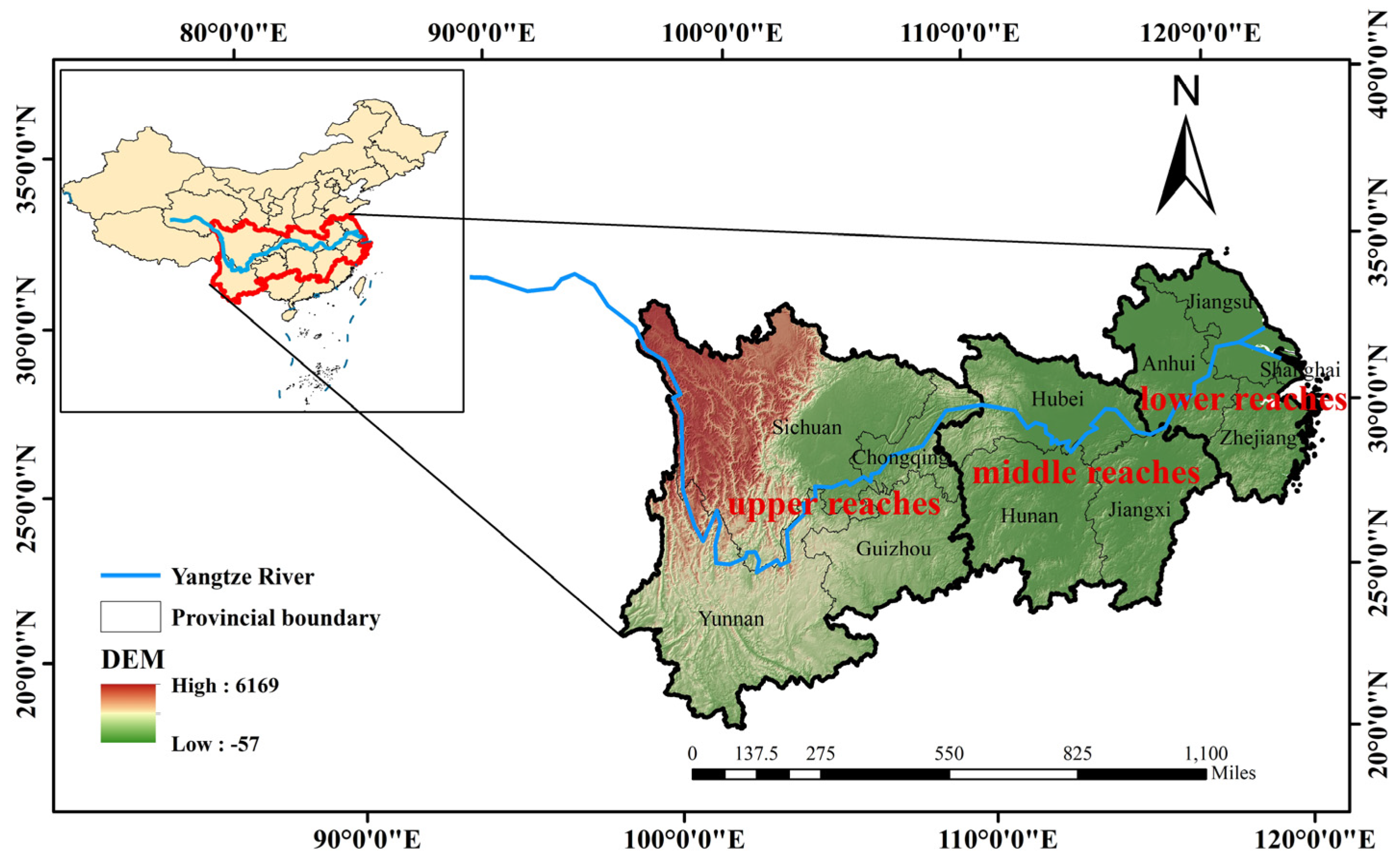
As illustrated in Figure 1, the YREB extends across China’s eastern, central, and western regions, serving as a pivotal spatial platform for the nation’s coordinated regional development and high-quality growth strategies. Spanning approximately 2.05 million km², the region is distributed along the main course of the Yangtze River. Following the regional division commonly adopted in previous studies [13,14], the YREB was divided into upper, middle, and lower reaches. The upper reaches include Chongqing Municipality and the provinces of Sichuan, Yunnan, and Guizhou; the middle reaches comprise Hubei, Hunan, and Jiangxi Provinces; and the lower reaches consist of Anhui, Jiangsu, Zhejiang Provinces, and Shanghai Municipality.

The YREB, situated in the subtropical monsoon climatic region, features diverse landform types and a pronounced west–east topographic gradient. Pronounced east–west gradients in precipitation, topography, and ecological conditions are observed across the region, accompanied by a significant spatial correlation between rainfall erosivity and the normalized difference vegetation index [15]. A systematic investigation of the evolutionary characteristics and driving forces of land use and landscape patterns across different regions in the YREB is of considerable practical significance for improving the understanding of regional human–land relationships and supporting territorial spatial optimization and high-quality development.

2.2. Data Sources

The datasets used in this study can be classified into four categories: land-use, topographic, climatic, and socioeconomic data. These datasets comprised land-use data, digital elevation model (DEM) data and DEM-derived slope data, mean annual temperature and precipitation data, as well as nighttime light (NTL) and gross domestic product (GDP) data. Detailed information on the datasets and their sources is summarized in

Table 1. Data sources.

Dataset	Resolution	Source
Digital elevation model (DEM)	1 km	http://gebco.net
Slope	1 km	ArcGIS 10.8 slope analysis
Mean annual temperature	1 km	http://data.tpdc.ac.cn
Mean annual precipitation	1 km
Gross domestic product (GDP) data	1 km	http://www.stats.gov.cn
Nighttime light (NTL) data	1 km	https://dataverse.harvard.edu
CLCD land-use data	30 m	https://zenodo.org/records/18180184 (accessed on 1 October 2025)

.

Land-use information was obtained from the China Land Cover Dataset (CLCD), developed by Wuhan University and publicly available for research applications [16]. The dataset provides annual land-cover maps of China at a spatial resolution of 30 m and was generated from Landsat imagery under a consistent classification framework. Previous assessments reported an overall classification accuracy of approximately 79% and a kappa coefficient greater than 0.70, demonstrating its reliability for long-term land-use change studies. Furthermore, the use of a unified classification system throughout the study period facilitates robust temporal comparisons among different years.

To capture the long-term evolution of land use in the study area, this study selects land use data from seven periods in 1993, 1998, 2003, 2008, 2013, 2018, and 2023. To align with the specific research scope and analytical requirements, all land use data are preprocessed on the ArcGIS 10.8 platform [8,17], including cropping and reclassification. Accordingly, six land cover types were identified: built-up land, forest land, cultivated land, water bodies, grassland, and unused land. Considering the large spatial extent of the YREB and the objective of analyzing long-term regional land-use dynamics, this classification scheme was considered sufficient to capture the dominant land-use transitions while ensuring temporal consistency across the study period.

3. Research Methods

3.1. Land Use Transfer Matrix Method

Widely employed in land-use change research, the land-use transfer matrix [18,19] quantitatively records conversions among different land-use categories over time. By revealing the direction, extent, and intensity of these transitions, it enables the identification of major land-use change patterns and provides a basis for exploring the factors associated with land-use dynamics. Assuming n land use categories, the land use transitions between different periods can be represented by an n × n matrix:

$$\mathrm{A}=\left[\begin{array}{cccc}{a}_{11}& a_{12}& \dots & a_{1n}\\ a_{21}& a_{22}& \dots & a_{2n}\\ ⋮& ⋮& \ddots & ⋮\\ a_{n1}& a_{n2}& \dots & a_{nn}\end{array}\right]$$

(1)

where a_ij denotes the area (in km²) of land transferred from type i to type j during the study period. The diagonal elements a_ii represent persistent land-use categories, while the off-diagonal entries record transitions among different land-use types. The row totals represent the area distribution of each land-use type at the initial time, while the column totals represent the corresponding distribution at the final time. The transfer matrix was generated through spatial overlay analysis of land-use maps from two periods in ArcGIS 10.8, which quantitatively identifies the source and destination of land-use conversions.

3.2. Grid-Based Method

The grid-based method [20,21] is a widely adopted spatial partitioning approach in landscape pattern research. Its fundamental principle involves dividing the study area into a series of regular grid cells of equal size, treating each cell as an independent spatial analysis unit. Within each grid cell, the composition of landscape types, the configuration characteristics, and the spatial structural parameters are quantitatively calculated. This method enables landscape pattern analysis under a unified scale, effectively circumventing the scale and edge effects arising from disparities in administrative district sizes or the intricate boundaries of natural units.

The study area spans a vast territory, and conducting landscape pattern analysis across such an expansive and geographically complex space presents notable challenges. If administrative divisions or natural geographical units are directly adopted as analytical units, it often leads to issues such as inconsistent scales, blurred boundaries, and deviations in landscape index calculations, thereby making it difficult to accurately capture the true characteristics of regional landscape patterns. Research on ecological risk assessment in the YREB has shown that the use of uniform spatial units is essential for conducting regional-scale comparative analyses and effectively revealing spatial differentiation patterns [22]. Similarly, studies on landscape ecological security have emphasized that regular spatial units can reduce the influence of administrative boundary discrepancies and improve the comparability of landscape pattern analyses across large regions [23]. Furthermore, fishnet-based grid analysis has been successfully applied to investigate the relationship between ecosystem service value and landscape patterns in the YREB, demonstrating the suitability of regular grids for characterizing regional spatial heterogeneity [24].

Considering the pronounced heterogeneity of the YREB and previous grid-based studies in the region, a 40 km × 40 km square grid was adopted as the basic analytical unit [25]. The selected grid size represents a compromise between capturing spatial variability and maintaining regional comparability. A smaller grid size is more likely to amplify local spatial variability and increase computational requirements, whereas a larger grid size may reduce the ability to capture landscape heterogeneity. Moreover, the 30 m spatial resolution of the CLCD dataset provides sufficient land-use information within each grid cell, thereby enabling stable and reliable computation of landscape metrics.

3.3. Selection of Landscape Pattern Index

As an important quantitative metric, the landscape pattern index is widely used to characterize landscape structure and spatial pattern dynamics. It enables the measurement of regional connectivity, fragmentation degree, and diversity across three hierarchical levels: patch, patch class, and landscape. This index has been widely employed in studies related to land use change, ecological risk evaluation, and ecosystem service responses [26,27]. Drawing on the analytical frameworks employed in existing landscape pattern studies at both regional and economic belt scales, and taking full account of the landscape features, land use change dynamics, and research objectives of the YREB [17], this study utilizes Fragstats 4.2 to perform a quantitative analysis of landscape patterns from both the landscape and class levels.

At the landscape level, eight metrics, including the number of patches (NP), patch density (PD), largest patch index (LPI), edge density (ED), contagion index (CONTAG), Shannon’s diversity index (SHDI), Shannon’s evenness index (SHEI), and aggregation index (AI), were selected to evaluate landscape fragmentation, spatial configuration, and compositional diversity across the study area. NP, PD, and ED primarily reflect the degree of landscape fragmentation and the complexity of landscape boundaries; LPI, AI, and CONTAG reflect the spatial aggregation and dominance characteristics of the landscape, whereas SHDI and SHEI describe the diversity and evenness of landscape types from a compositional perspective. These metrics jointly display the comprehensive features of the landscape pattern.

At the class level, percent of landscape (PLAND), landscape shape index (LSI), patch cohesion index (COHESION), number of patches (NP), edge density (ED), and aggregation index (AI) were selected to assess the composition, shape characteristics, connectivity, aggregation, and fragmentation of individual land-use types. PLAND represents area composition; NP and ED characterize fragmentation and edge features; LSI reflects patch shape complexity; and COHESION and AI describe connectivity and aggregation patterns, respectively. The corresponding formulas are listed in

Table 2. The selected landscape metrics.

Name	Formula	Name	Formula	Type
Number of Patches	${\mathrm{NP}}_i={\displaystyle \sum _{i=1}^m{n}_i}$	Edge Density	${\mathrm{ED}}_i={\displaystyle \frac{{\mathrm{E}}_i}{\mathrm{A}}}$	Landscape, Patch
Patch Density	$\mathrm{PD}={\displaystyle \frac{\mathrm{NP}}{\mathrm{A}}}$	Largest Patch Index	$\mathrm{LPI}={\displaystyle \frac{{\max (\mathrm{A}}_{\mathrm{i}})}{\mathrm{A}}}$	Landscape
Shannon’s Evenness Index	$\mathrm{SHEI}={\displaystyle \frac{-{\displaystyle \sum _{\mathrm{i}=1}^{\mathrm{m}}{\mathrm{P}}_{\mathrm{i}}{\mathrm{lnP}}_{\mathrm{i}}}}{\mathrm{lnm}}}$	Shannon’s Diversity Index	$\mathrm{SHDI}=-{\displaystyle \sum _{\mathrm{i}=1}^{\mathrm{m}}{\mathrm{P}}_{\mathrm{i}}{\mathrm{lnP}}_{\mathrm{i}}}$	Landscape
Percentage of Landscape	$\mathrm{PLAND}={\displaystyle \frac{{\displaystyle {\sum }_{\mathrm{j}=1}^{{\mathrm{n}}_{\mathrm{i}}}{\mathrm{a}}_{\mathrm{ij}}}}{\mathrm{A}}}$	Landscape Shape Index	$\mathrm{LSI}={\displaystyle \frac{{\mathrm{E}}_{\mathrm{i}}}{2\sqrt{\mathsf{\pi }\times {\displaystyle {\sum }_{\mathrm{j}=1}^{{\mathrm{n}}_{\mathrm{i}}}{\mathrm{a}}_{\mathrm{ij}}}}}}$	Patch
Aggregation Index	$\mathrm{AI}={\displaystyle \frac{{\displaystyle \sum {\mathrm{g}}_{\mathrm{ii}}}}{{\displaystyle \sum {\max (\mathrm{g}}_{\mathrm{ii}})}}}$			Landscape, Patch
Contagion Index	$\mathrm{CONTAG}=\left[1+{\displaystyle \frac{{\displaystyle {\sum }_{\mathrm{i}=1}^{\mathrm{n}}}{\displaystyle {\displaystyle }{\sum }_{\mathrm{k}=1}^{\mathrm{n}}\left[{\mathrm{P}}_{\mathrm{i}}\frac{{\mathrm{g}}_{\mathrm{ik}}}{{\displaystyle {\sum }_{\mathrm{k}=1}^{\mathrm{n}}{\mathrm{g}}_{\mathrm{ik}}}}\right]\left[{\ln (\mathrm{P}}_{\mathrm{i}})\frac{{\mathrm{g}}_{\mathrm{ik}}}{{\displaystyle {\sum }_{\mathrm{k}=1}^{\mathrm{n}}{\mathrm{g}}_{\mathrm{ik}}}}\right]}}{2\ln \left(\mathrm{n}\right)}}\right]$			Landscape
Patch Cohesion Index	$\mathrm{COHESION}=\left[1-{\displaystyle \frac{{\displaystyle {\sum }_{\mathrm{j}=1}^{{\mathrm{n}}_{\mathrm{i}}}{\mathrm{p}}_{\mathrm{ij}}}}{{\displaystyle {\sum }_{\mathrm{j}=1}^{{\mathrm{n}}_{\mathrm{i}}}{\mathrm{p}}_{\mathrm{ij}}}\sqrt{{\mathrm{a}}_{\mathrm{ij}}}}}\right]\times {\left[1-{\displaystyle \frac{1}{\sqrt{\mathrm{A}}}}\right]}^{-1}$			Patch

Note: A = total landscape area; m and n = number of landscape classes; n_i = number of patches of class i; a_ij = area of patch j in class i; p_ij = perimeter of patch j in class i; E_i = total edge length of class i; max(A_i) = area of the largest patch in the landscape; P_i = proportion of landscape occupied by class i; g_ii = number of like adjacencies between pixels of class i; g_ik = number of adjacencies between pixels of classes i and k; max(g_ii) = maximum possible number of like adjacencies for class i.

.

3.4. Geodetector

Geodetector [28] is a statistical method widely used to detect spatial heterogeneity and reveal its underlying driving factors. This method is especially suitable for geographical phenomena featured by significant spatial heterogeneity, such as landscape pattern evolution and environmental process analysis, and has been extensively used in studies related to ecological environments and regional sustainable development [29].

The factor detector was applied to assess the explanatory power of individual factors for the spatial differentiation of landscape pattern metrics. Based on the theory of spatial stratified heterogeneity, a factor is considered to have stronger explanatory power when the variance of the dependent variable within each stratum is substantially lower than that among strata. The explanatory contribution of each factor was quantified using the q-statistic, with larger q-values indicating stronger associations with the observed spatial variation in landscape pattern metrics. The formula is expressed as follows:

$$\mathrm{q}=1-{\displaystyle \frac{{\displaystyle \sum _{\mathrm{h}=1}^{\mathrm{L}}{\mathrm{N}}_{\mathrm{h}}{\mathsf{\sigma }}_{\mathrm{h}}^2}}{{\mathrm{N}\mathsf{\sigma }}^2}}=1-{\displaystyle \frac{\mathrm{SSW}}{\mathrm{SST}}}$$

(2)

$$\mathrm{SSW}={\displaystyle \sum _{\mathrm{h}=1}^{\mathrm{L}}{\mathrm{N}}_{\mathrm{h}}{\mathsf{\sigma }}_{\mathrm{h}}^2}, {\mathrm{SST}=\mathrm{N}\mathsf{\sigma }}^2$$

(3)

In the equation, L represents the number of strata of the independent variable X, and h denotes a specific stratum. N_h and N refer to the sample sizes in stratum h and the entire study area, respectively. ${\sigma }_h^2$ and ${\sigma }^2$ indicate the variances of the dependent variable Y within stratum h and across the whole region, respectively. SSW denotes the within-stratum sum of variances, whereas SST represents the total variance.

The interaction detector is employed to analyze the interactions between two driving factors under their joint influence. By comparing the discrepancy between the superimposed effect of the two factors and their individual effects, it enables the determination of whether an enhancement, weakening, or independent effect exists between them. Interactive detection can reveal the synergistic or inhibitory mechanisms between different natural and socioeconomic factors, thereby facilitating a profound understanding of the complex driving-force system underlying landscape pattern evolution. This approach offers significant advantages in multi-factor coupling analysis [30]. The interaction types were classified according to the relationships among q(X₁), q(X₂), and q(X₁∩X₂), as summarized in

Table 3. Criteria and types of interaction effects in interaction detection.

Interaction	Basis for Judgment
Nonlinear Weakening	$\mathrm{q}\left(\mathrm{X}1\cap \mathrm{X}2\right)<\mathrm{Min}\left(\mathrm{q}\left(\mathrm{X}1\right),\mathrm{q}\left(\mathrm{X}2\right)\right)$
Single-factor Nonlinear Weakening	$\mathrm{Min}\left(\mathrm{q}\left(\mathrm{X}1\right),\mathrm{q}\left(\mathrm{X}2\right)\right)<\mathrm{q}\left(\mathrm{X}1\cap \mathrm{X}2\right)<\mathrm{Max}\left(\mathrm{q}\left(\mathrm{X}1\right),\mathrm{q}\left(\mathrm{X}2\right)\right)$
Bi-enhancement	$\mathrm{q}\left(\mathrm{X}1\cap \mathrm{X}2\right)>\mathrm{Max}\left(\mathrm{q}\left(\mathrm{X}1\right),\mathrm{q}\left(\mathrm{X}2\right)\right)$
Independent	$\mathrm{q}\left(\mathrm{X}1\cap \mathrm{X}2\right)=\mathrm{q}\left(\mathrm{X}1\right)+\mathrm{q}\left(\mathrm{X}2\right)$
Nonlinear Enhancement	$\mathrm{q}\left(\mathrm{X}1\cap \mathrm{X}2\right)>\mathrm{q}\left(\mathrm{X}1\right)+\mathrm{q}\left(\mathrm{X}2\right)$

.

4. Results and Analysis

4.1. Land Use Type Transformation

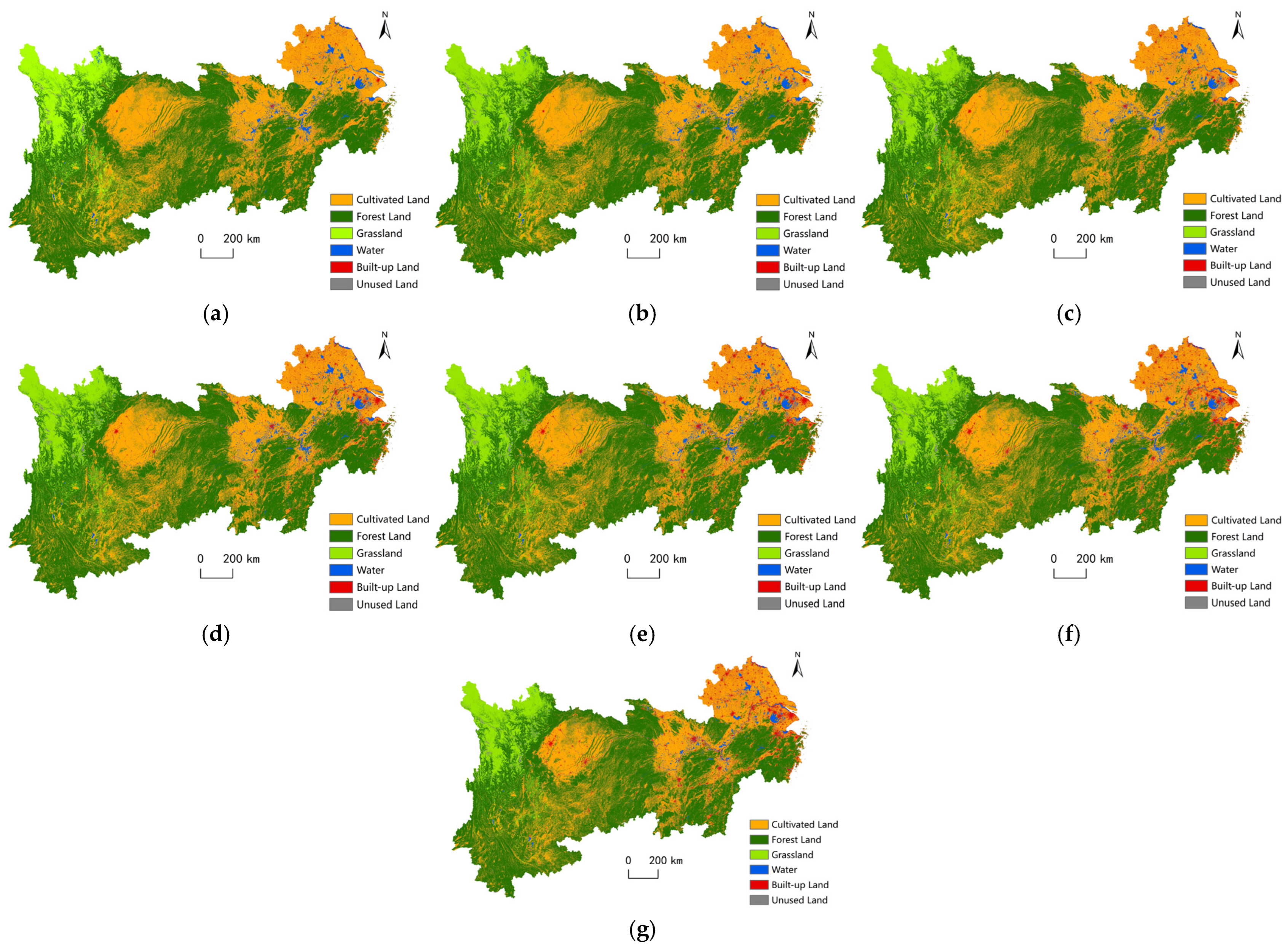
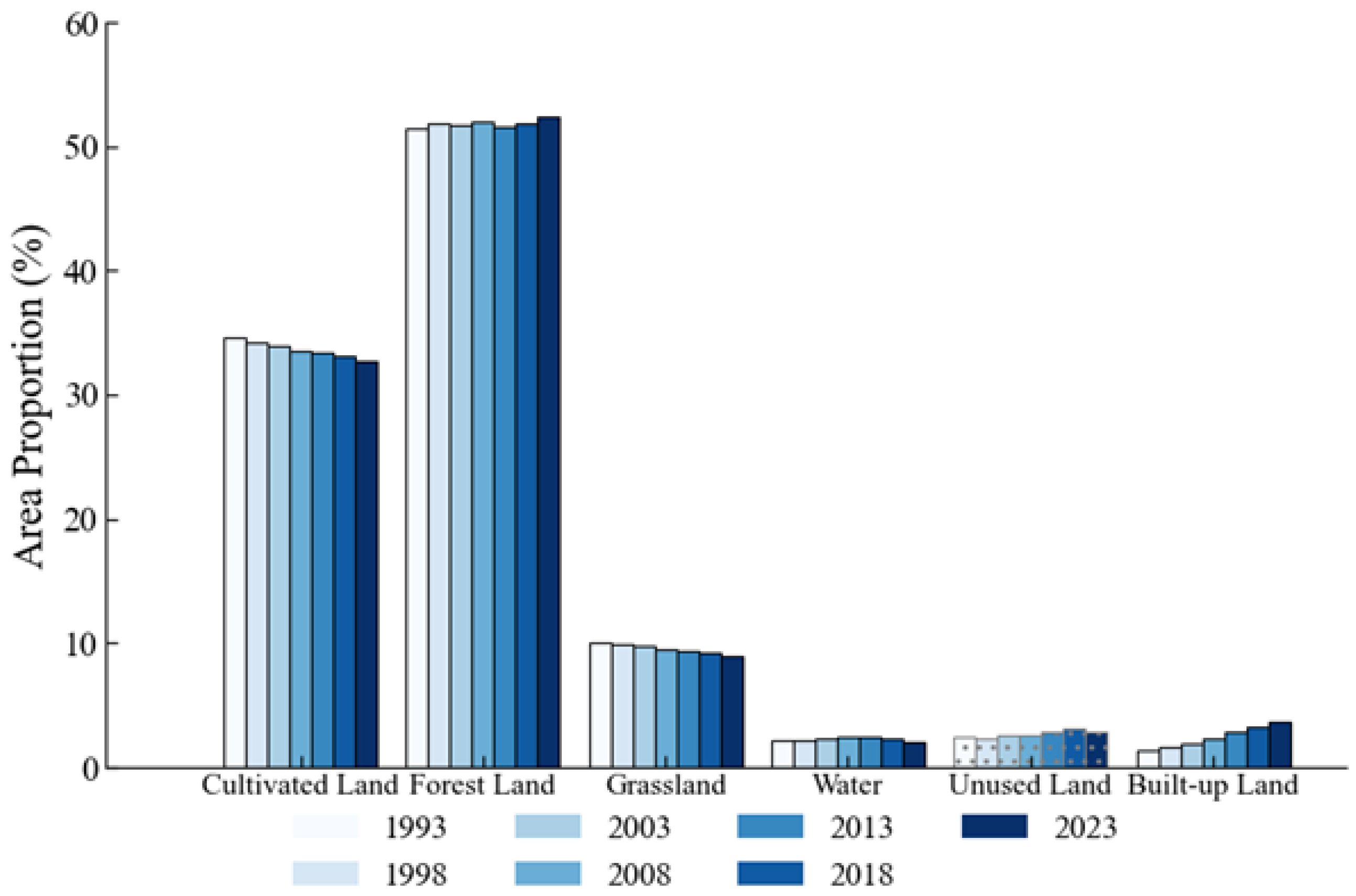
The proportional changes in area for each land use type from 1993 to 2023 are illustrated in Figure 2, while the spatial distribution characteristics of land use in representative years are presented in Figure 3. The overall land-use composition of the YREB exhibited limited variation during the study period, with cultivated land and forest land remaining the predominant land-use categories. Collectively, these two types constituted more than 85% of the total study area throughout the period. From the perspective of temporal variation, the cultivated land area and its proportion exhibited a persistent downward trend. The area of cultivated land decreased from 708,071.39 km² in 1993 to 670,206.24 km² in 2023, and its proportion declined from 34.63% to 32.78%. The area of forest land increased from 1,053,239.75 km² in 1993 to 1,070,472.12 km² in 2023, with its proportion rising from 51.51% to 52.36%. It remained the dominant land use type with the largest areal share across the study region. Meanwhile, the grassland area and its proportion showed a continuous declining trend. Its area declined from 204,940.95 km² in 1993 to 182,557.57 km² in 2023, representing a reduction in proportional coverage from 10.02% to 8.93%. Changes in grassland were relatively limited over the study period, although its area displayed a gradual declining trend. Water bodies showed marked interannual fluctuations, whereas unused land consistently accounted for only a small share of the total area. By contrast, built-up land experienced the most pronounced expansion in both area and proportion, increasing from 27,715.03 km² in 1993 to 73,772.29 km² in 2023, with its share rising from 1.36% to 3.61%. Notably, the growth rate accelerated markedly after 2008, rendering built-up land the most dynamically expanding land use type throughout the study period.

Spatially, cultivated land was predominantly distributed across the major plains and basin regions of the YREB, including the Sichuan Basin, Jianghan Plain, Dongting Lake Plain, Poyang Lake Plain, and the Yangtze River Delta. Comparison of the land-use maps across different years shows that cultivated land declined most noticeably in rapidly urbanizing metropolitan areas, where urban expansion progressively replaced agricultural land. Forest land consistently represented the largest land-use category during the study period and was predominantly distributed in the mountainous and hilly regions of the upper and middle reaches of the YREB. Both the spatial distribution maps and area statistics indicate a slight increase in forest land between 1993 and 2023. Grassland was mainly distributed in the western YREB and experienced a modest but persistent decline during the study period. Conversely, built-up land expansion was concentrated in the major urban agglomerations of the region, notably the Yangtze River Delta, the Wuhan Metropolitan Area, and the Chengdu–Chongqing Economic Circle. By 2023, built-up land exhibited a more aggregated and continuous spatial pattern around major cities than in 1993. The total area of built-up land increased by 46,057.26 km² over the study period, representing the largest net increase among all land-use types and indicating the substantial impact of urbanization on regional land-use dynamics. Although the overall land-use structure of the YREB remained relatively stable during 1993–2023, distinct regional differences were observed among the upper, middle, and lower reaches. In the upper reaches, land-use composition was dominated by forest land and grassland, and land-use changes were relatively limited, which may be related to ecological conservation efforts and constraints imposed by natural environmental conditions. The middle reaches exhibited a transitional pattern, where cultivated land remained an important component while built-up land continued to expand, reflecting the combined influence of agricultural development and socioeconomic growth. In contrast, the lower reaches experienced the most intensive land-use transformation, characterized by rapid expansion of built-up land and notable reductions in cultivated land associated with intensive urban development. These regional differences suggest that land-use evolution in the YREB was influenced by the combined effects of ecological conditions, resource availability, and socioeconomic development intensity. Overall, these spatial and temporal characteristics of land-use change provide an important foundation for subsequent analyses of landscape pattern evolution and regional landscape differentiation.

4.2. Analysis of Land Use Transfer Matrix

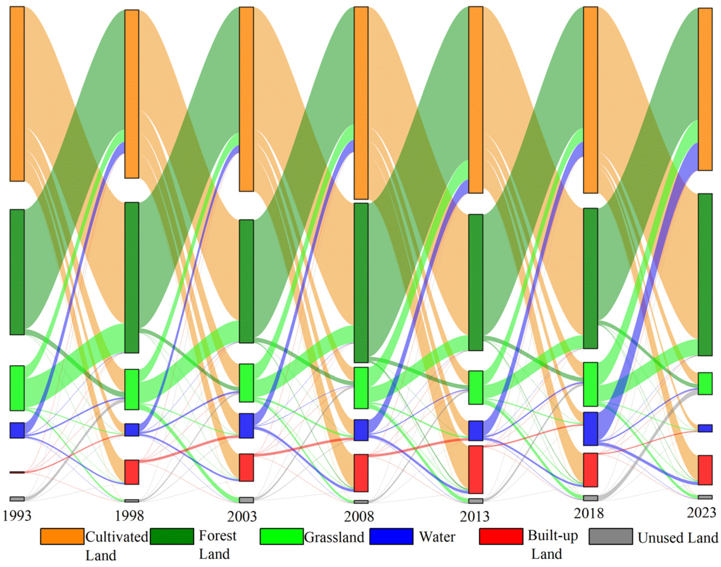
Figure 4 presents the characteristics of land use transitions in the study area over the period 1993–2023, revealing pronounced differences in the dominant transfer pathways and evolutionary mechanisms across different stages. During the entire study period, land-use transitions in the YREB were primarily characterized by the continuous expansion of built-up land and the redistribution of agricultural and ecological land. The most dominant long-term conversion pathway was the transformation of cultivated land into built-up land, reflecting the increasing influence of urbanization and infrastructure development. Meanwhile, bidirectional exchanges among cultivated land, forest land, and grassland indicated the combined effects of agricultural adjustment and ecological restoration. The land use transitions in the YREB have undergone an evolutionary process that progressively shifted from a phase dominated by ecological and agricultural adjustment toward a stage characterized by human-driven land-use transformation.

(1)

From 1993 to 1998, land use transfer was predominantly concentrated among cultivated land, forest land, and grassland, representing a typical process of natural resource reallocation. A bidirectional conversion relationship was evident between cultivated land and forest land, whereas grassland presented a net inflow characteristic. This indicated that land use changes during this stage are predominantly driven by agricultural structural adjustment and ecological restoration, with the influence of human construction activities remaining relatively subdued and the overall intensity of regional development being low.

(2)

From 1998 to 2008, land-use changes gradually intensified, representing a transitional stage between ecological adjustment and rapid urbanization. Although cultivated land, forest land, and grassland remained the major components involved in land conversion, the expansion of built-up land became increasingly evident. The increasing conversion of cultivated land into built-up land indicated that human activities gradually became an important factor shaping regional land-use patterns.

(3)

From 2008 to 2013, the land use transfer pattern underwent significant changes, with built-up land emerging as an important inflow type. This transition suggests that the study area had entered a phase of rapid urbanization. A considerable amount of cultivated land was converted into built-up land, and forest land also contributed to this conversion to some extent, indicating the coexistence of urban expansion and ecological adjustment. Compared to the previous stage, land use change has gradually transitioned from natural evolution to human-dominated transformation, accompanied by a significant increase in the intensity of spatial development.

(4)

From 2013 to 2018, built-up land expansion became increasingly prominent and represented the largest land-use transition during the study period. The persistent conversion of cultivated land to built-up land, together with the rising intensity of this transition, reflects the rapid progression of urbanization and infrastructure development. Meanwhile, forest land and grassland exhibited relatively minor changes, resulting in a land-use pattern characterized by the continued expansion of built-up land and the overall stability of ecological land. Collectively, these changes suggest a gradual shift in regional development from extensive land expansion toward a more structurally optimized development trajectory.

(5)

From 2018 to 2023, the overall land use change intensity showed a relatively stable and flat trend; nevertheless, built-up land continued to exhibit sustained net growth. Cultivated land remained the primary source of built-up land expansion, whereas forest land maintained a relatively dynamic equilibrium. This indicated that land use was gradually transitioning toward a “development-protection coordination” paradigm. At this stage, land-use change gradually transitioned from rapid expansion to high-quality development, while the regional land-use structure became increasingly stable.

4.3. Spatiotemporal Dynamics of Landscape Patterns

4.3.1. Analysis of Index Changes at the Landscape Level

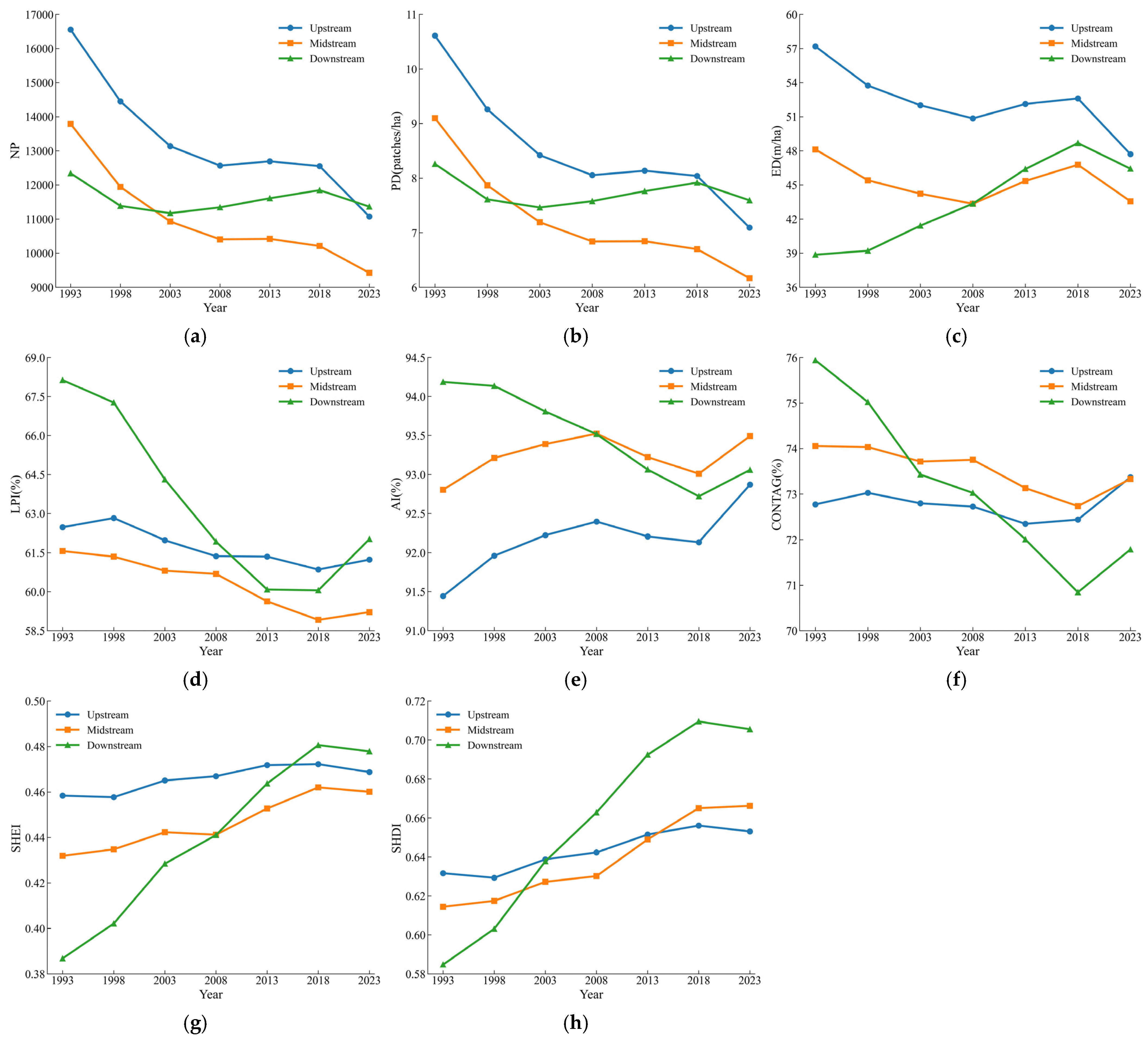
NP, PD and ED serve as the core indicators for characterizing the degree of landscape fragmentation. As shown in panels (a), (b), and (c) in Figure 5, the NP in the upper reaches decreased significantly from 16,553 to 11,073 between 1993 and 2023, representing a decline of 33.1%. Over the same period, PD decreased from 10.610/ha to 7.093/ha, while ED decreased from 57.185 m/ha to 47.709 m/ha. Collectively, all three indicators exhibited a consistent and continuous downward trend. This indicated a decline in the number of landscape patches, a reduction in edge complexity, a weakening of landscape fragmentation, and a trend toward a more complete and continuous landscape structure. NP decreased from 13,789 to 9422, and PD decreased from 9.099/ha to 6.167/ha in the middle reaches, with the magnitude of decline being slightly smaller than that observed in the upper reaches. However, ED exhibited pronounced fluctuation characteristics, ranging between 43.3 and 48.1 m/ha, indicating that despite the reduction in patch numbers, the spatial contact interfaces among land use types remained notably complex. This feature indicated that the landscape pattern in the middle reaches remained in a stage of ongoing adjustment, shaped by the dual and intertwined influences of urban expansion and agricultural structural transformation. During the study period, the overall changes in NP and PD in the lower reaches were relatively modest; however, ED exhibited a pronounced upward trend after 2003, rising from 41.420 m/ha in 2003 to 46.427 m/ha in 2023, with a peak value of 48.686 m/ha recorded in 2018, thereby indicating a marked increase in landscape edge length. It showed that landscape fragmentation in the lower reaches was mainly manifested through the enhancement of edge complexity, rather than a simple increase in patch number, which reflected the typical characteristics of frequent land-use transformation in highly urbanized areas.

The largest patch index (LPI) and agglomeration index (AI) can be employed to characterize the spatial dominance of the predominant land use type and its degree of agglomeration, respectively. Figure 5, panels (d) and (e), indicate that the LPI in the upper reaches persists at levels between 60% and 63% over an extended period. While a slight downward trend was observable, the overall magnitude remains markedly higher than that of the middle reaches, signifying that ecological land categories, particularly forest land, have consistently maintained a dominant position. AI remained consistently stable, fluctuating within a narrow range of 91% to 93%, which indicated that the spatial aggregation of landscape patches was notably strong and the overall pattern stability remained at a high level. The LPI in the middle reaches decreased from 61.566% to 59.215%, exhibiting a gradual downward trend that reflected a weakening of the dominant patch area. However, the AI value consistently remained around 93%, indicating that despite structural adjustments in landscape types, the overall spatial aggregation pattern remained relatively stable. This revealed an evolutionary characteristic of “structural change without significant spatial dispersion”. In the lower reaches, the LPI exhibited the most pronounced decline, falling from 68.135% to 62.023%, while the AI also decreased, from 94.188% to 93.058%. The results indicated that the continuity of the originally dominant patches in the lower reaches was significantly weakened, and the landscape structure has shifted from single-dominance to multi-type coexistence, which reflected the profound reshaping effect of rapid urbanization on the regional landscape pattern.

The CONTAG and SHEI describe, at the holistic level, the level of landscape spatial aggregation and the interlacing of landscape types. As shown in panels (f) and (g) of Figure 5, the CONTAG values of the upper reaches consistently remained between 72% and 73%, exhibiting only a slight fluctuation range; meanwhile, the SHEI stabilized within the range of 0.45–0.47. These results indicated that the distribution of landscape types was relatively concentrated, the spatial structure remained stable, and the overall continuity was notably strong. The CONTAG value in the middle reaches exhibited a gradual decline from 74.056% to 73.330%, while the overall SHEI showed an upward trend. These changes reflected an increasing degree of spatial interlace among different types, indicating an evolutionary trajectory of the landscape pattern from relative agglomeration toward dispersion. The CONTAG value decreased significantly from 75.944% to 71.786%, while SHEI increased significantly from 0.387 to 0.478 in the lower reaches. These changes indicated that landscape types became highly mixed and spatial heterogeneity was markedly enhanced, which reflected the most intense landscape spatial reconstruction observed within the region.

As shown in Figure 5h, the SHDI across all three major regions exhibited an upward trend; however, the rates of increase varied markedly among them. SHDI in the upper reaches increased from 0.632 to 0.653, with only a modest increase indicating a slight enhancement in landscape diversity while the overall ecological dominance pattern remained relatively stable. This trend was accompanied by only minor changes in land-use composition and area distribution, suggesting limited variation in landscape richness and evenness. The SHDI in the middle reaches increased from 0.615 to 0.666, indicating that landscape types became more evenly distributed and that the relative dominance among different land-use categories gradually weakened. Combined with the increase in SHEI and the decline in CONTAG, this pattern reflects a growing degree of spatial interspersion among landscape types. The lower reaches exhibited the most pronounced increase in SHDI, rising from 0.585 to 0.706. This substantial increase indicates a marked enhancement in both the compositional diversity and evenness of landscape types. Meanwhile, the concurrent decrease in LPI, CONTAG, and AI, together with the increase in ED and SHEI, suggests that the increase in diversity was accompanied by greater spatial heterogeneity and a more complex landscape configuration. Overall, the lower reaches experienced the most significant changes in landscape diversity and spatial structure during the study period.

4.3.2. Analysis of Index Change at the Class Level

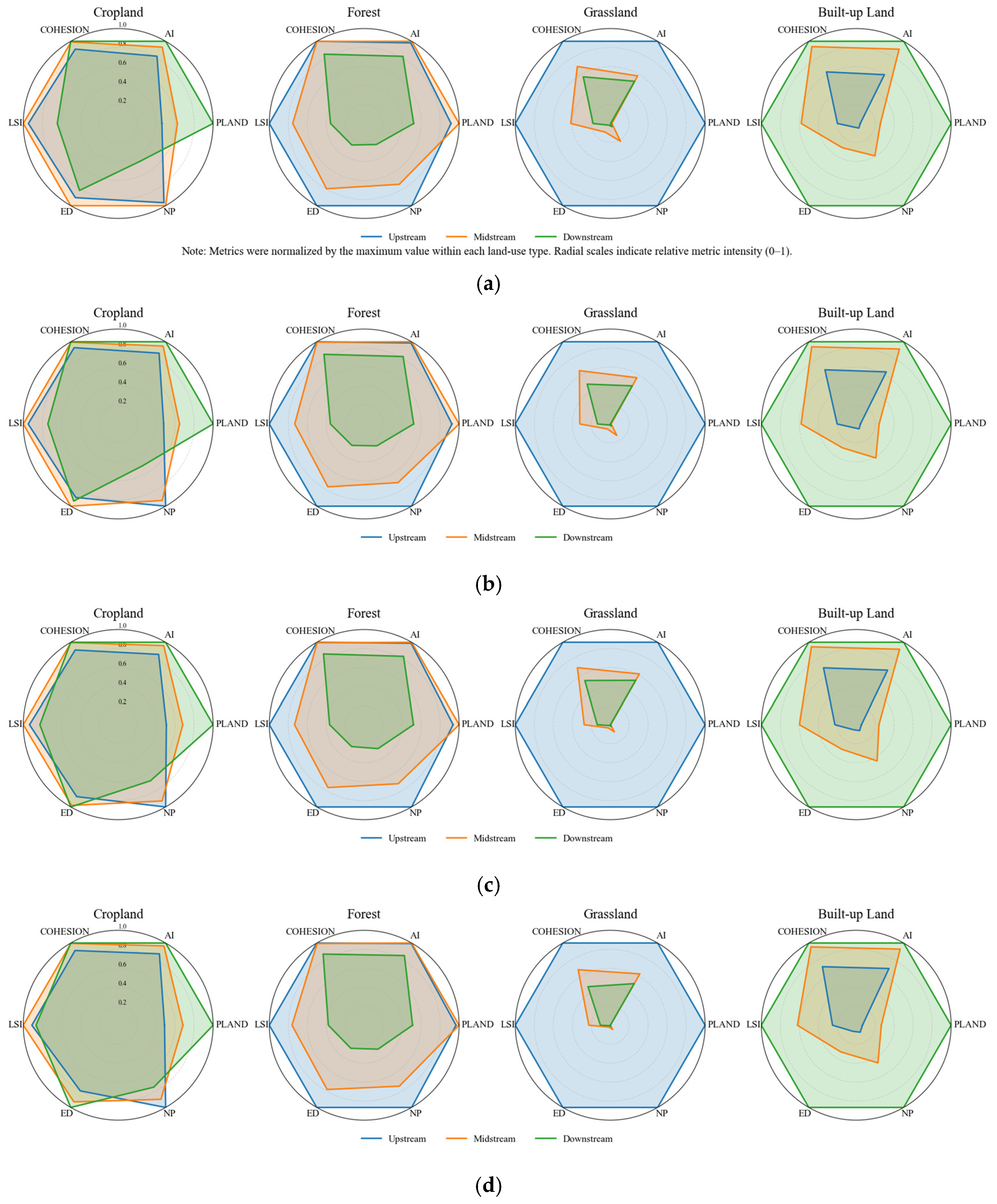
Figure 6 presents radar charts integrating six class-level landscape metrics for cropland, forest land, grassland, and built-up land in 1993 and 2023. These four land-use categories collectively constituted more than 95% of the total area of the YREB throughout the study period and therefore represented the principal components of the regional landscape. By integrating indicators of area composition, fragmentation, shape complexity, connectivity, and aggregation, the radar charts facilitate a comparative assessment of landscape characteristics among different land-use types and regions. The resulting metric profiles further enable the evaluation of landscape evolution patterns associated with individual land-use types across the upper, middle, and lower reaches of the YREB.

The lower reaches consistently exhibited the highest PLAND values, remaining above 50% throughout the study period, whereas the corresponding PLAND values in the middle and upper reaches remained at approximately 35% and 25%, respectively. Between 1993 and 2023, cropland PLAND declined in all three regions, with the largest decrease occurring in the lower reaches. The NP, ED, and LSI values of cropland showed contrasting trends among regions. In the upper and middle reaches, these indicators generally decreased from 1993 to 2023, indicating reductions in fragmentation and boundary complexity. In contrast, the lower reaches experienced increases in NP, ED, and LSI, suggesting a more fragmented and irregular cropland pattern. Meanwhile, COHESION and AI values generally showed a downstream-dominant pattern during the study period. The lower reaches tended to exhibit higher connectivity and aggregation levels than the middle and upper reaches, while the upper reaches were characterized by relatively lower values.

Forest land consistently represented the principal ecological landscape type in both the upper and middle reaches. The middle reaches maintained the highest forest coverage, with PLAND remaining relatively stable at approximately 58%–59%, while the upper reaches showed a gradual increase from 54.14% in 1993 to 56.44% in 2023. In contrast, forest PLAND in the lower reaches decreased slightly during the study period. The NP, ED, and LSI values of forest land generally declined across all regions, particularly in the upper reaches, indicating reduced fragmentation and simplified patch morphology. At the same time, AI and COHESION values remained consistently high and showed slight increases over time. Compared with the upper and middle reaches, the lower reaches exhibited lower NP, ED, and LSI values throughout the study period, reflecting a relatively simpler forest landscape structure.

Grassland exhibited the strongest regional heterogeneity among all land-use types. Grassland was overwhelmingly concentrated in the upper reaches, with PLAND exceeding 16% in 2023, whereas grassland occupied less than 0.1% of the total area in both the middle and lower reaches. The upper reaches consistently recorded the highest NP, ED, and LSI values, indicating a more fragmented and morphologically complex grassland landscape. However, all three indicators decreased markedly from 1993 to 2023, while AI and COHESION increased continuously, reflecting enhanced connectivity and aggregation of grassland patches. In the middle and lower reaches, grassland PLAND, NP, ED, and LSI all remained at relatively low levels and continued to decline over time. The radar charts further show that regional differences in grassland landscape structure became more pronounced between 1993 and 2023, with the upper reaches maintaining a dominant position in terms of both area proportion and landscape complexity.

Built-up land experienced the most pronounced changes among all land-use types during the study period. The lower reaches exhibited the highest PLAND values, increasing from 5.09% in 1993 to 12.81% in 2023. The middle reaches also showed substantial growth, with PLAND increasing from 1.30% to 3.39%, whereas the upper reaches maintained comparatively low levels despite a continuous increase. The NP, ED, and LSI values of built-up land increased in all three regions, indicating increasing patch numbers, edge density, and shape complexity. These increases were particularly evident in the lower reaches, where the values remained substantially higher than those in the upper and middle reaches. Meanwhile, AI and COHESION increased continuously across all regions, suggesting enhanced connectivity and aggregation of built-up land patches. By 2023, the lower reaches exhibited the highest values for nearly all landscape metrics, highlighting their distinctive landscape structure compared with the other two regions.

Overall, the class-level landscape metrics revealed distinct differences among land-use types and regions within the YREB. Cropland and grassland exhibited markedly different fragmentation patterns across regions, particularly between the upper and lower reaches, while forest land maintained relatively stable and highly connected landscape structures throughout the study period. Built-up land showed the most significant changes, characterized by simultaneous increases in area proportion, connectivity, and landscape complexity. The comparison between 1993 and 2023 further indicates that the spatial differentiation of landscape patterns among regions became increasingly pronounced over time, particularly for cropland, grassland, and built-up land.

4.4. Analysis of Driving Factors of Landscape Index Changes

From 1993 to 2023, land-use landscape patterns in the YREB exhibited distinct temporal and spatial variations. To explore the factors associated with these changes, six natural and socioeconomic variables were selected based on regional characteristics and data availability for subsequent Geodetector analysis. The dependent variable Y was selected based on the appropriate factors characterizing the upper, middle, and lower reaches, while the independent variable X encompassed the following six factors: digital elevation model (X1), slope (X2), mean annual temperature (X3), mean annual precipitation (X4), nighttime light (X5), and GDP (X6). The factors were discretized, and both the natural factors and the socio-economic factors were categorized into four classes. Before applying the Geodetector model, continuous driving factors were discretized using the Natural Breaks (Jenks) method, which organizes observations into relatively homogeneous classes by minimizing variability within classes and increasing differences among classes. To ensure comparability among variables and satisfy the requirements of the Geodetector model, both the natural and socio-economic factors were uniformly divided into four classes. All input datasets were resampled to achieve a consistent spatial resolution of 1 km and projected onto a unified Albers_Conic_Equal_Area coordinate system. To ensure spatial consistency between the dependent and explanatory variables, the 40 km × 40 km grid used for landscape metric calculation was adopted as the analytical unit. The mean value of each driving factor within each grid cell was calculated using zonal statistics in ArcGIS 10.8 and subsequently linked to the corresponding landscape metric values for Geodetector analysis.

4.4.1. Analysis of Single-Factor Detection

To avoid redundancy among multiple landscape metrics and to better represent the dominant dimensions of landscape change in each reach, one representative landscape metric was selected for the Geodetector analysis. The selection was based on the results of the preceding landscape-pattern analysis, which revealed distinct regional characteristics of landscape evolution across the upper, middle, and lower reaches of the YREB. Specifically, changes in the upper reaches were primarily reflected in the adjustment of patch morphology and edge complexity; therefore, ED was selected to characterize landscape structural variation. In the middle reaches, landscape evolution was mainly associated with increasing fragmentation caused by agricultural restructuring and urban expansion, making NP an appropriate indicator for capturing changes in patch configuration. In the lower reaches, where urbanization was more advanced and land-use types were highly mixed, changes were mainly reflected in landscape diversity and compositional heterogeneity; thus, SHDI was selected as the representative metric. To evaluate the robustness of this representative-metric selection strategy, additional Geodetector analyses were conducted using the remaining landscape metrics, and the results are provided in Appendix A (

Table A1. Factor detection of Edge Density (ED) changes in the middle reaches.

Driving Factors	1993		1998		2003		2008		2013		2018		2023
	q	p	q	p	q	p	q	p	q	p	q	p	q	p
X1	0.047	0.000	0.070	0.000	0.095	0.000	0.140	0.000	0.149	0.000	0.181	0.000	0.229	0.000
X2	0.124	0.000	0.157	0.000	0.189	0.000	0.239	0.000	0.251	0.000	0.273	0.000	0.314	0.000
X3	0.054	0.000	0.059	0.000	0.074	0.000	0.103	0.000	0.090	0.000	0.116	0.000	0.140	0.000
X4	0.103	0.000	0.104	0.000	0.104	0.000	0.097	0.000	0.105	0.000	0.099	0.000	0.086	0.000
X5	0.061	0.000	0.083	0.000	0.099	0.000	0.131	0.000	0.140	0.000	0.159	0.000	0.192	0.000
X6	0.037	0.000	0.060	0.000	0.078	0.000	0.116	0.000	0.119	0.000	0.125	0.000	0.151	0.000

,

Table A2. Factor detection of Edge Density (ED) changes in the lower reaches.

Driving Factors	1993		1998		2003		2008		2013		2018		2023
	q	p	q	p	q	p	q	p	q	p	q	p	q	p
X1	0.321	0.000	0.389	0.000	0.431	0.000	0.457	0.000	0.472	0.000	0.451	0.000	0.449	0.000
X2	0.266	0.000	0.311	0.000	0.337	0.000	0.359	0.000	0.360	0.000	0.340	0.000	0.344	0.000
X3	0.032	0.035	0.035	0.026	0.033	0.032	0.031	0.042	0.030	0.045	0.028	0.057	0.037	0.019
X4	0.254	0.000	0.314	0.000	0.360	0.000	0.364	0.000	0.405	0.000	0.398	0.000	0.417	0.000
X5	0.051	0.004	0.082	0.000	0.137	0.000	0.192	0.000	0.225	0.000	0.207	0.000	0.192	0.000
X6	0.103	0.000	0.142	0.000	0.220	0.000	0.270	0.000	0.310	0.000	0.289	0.000	0.275	0.000

,

Table A3. Factor detection of Number of Patches (NP) changes in the upper reaches.

Driving Factors	1993		1998		2003		2008		2013		2018		2023
	q	p	q	p	q	p	q	p	q	p	q	p	q	p
X1	0.300	0.000	0.284	0.000	0.288	0.000	0.290	0.000	0.298	0.000	0.304	0.000	0.299	0.000
X2	0.027	0.000	0.028	0.000	0.025	0.000	0.026	0.000	0.029	0.000	0.027	0.000	0.017	0.005
X3	0.259	0.000	0.254	0.000	0.242	0.000	0.230	0.000	0.225	0.000	0.220	0.000	0.199	0.000
X4	0.118	0.000	0.118	0.000	0.124	0.000	0.129	0.000	0.139	0.000	0.147	0.000	0.156	0.000
X5	0.169	0.000	0.164	0.000	0.170	0.000	0.185	0.000	0.204	0.000	0.207	0.000	0.194	0.000
X6	0.198	0.000	0.188	0.000	0.182	0.000	0.181	0.000	0.186	0.000	0.182	0.000	0.156	0.000

,

Table A4. Factor detection of Number of Patches (NP) changes in the lower reaches.

Driving Factors	1993		1998		2003		2008		2013		2018		2023
	q	p	q	p	q	p	q	p	q	p	q	p	q	p
X1	0.152	0.000	0.180	0.000	0.211	0.000	0.230	0.000	0.240	0.000	0.238	0.000	0.231	0.000
X2	0.201	0.000	0.240	0.000	0.279	0.000	0.297	0.000	0.304	0.000	0.306	0.000	0.305	0.000
X3	0.107	0.000	0.107	0.000	0.107	0.000	0.104	0.000	0.096	0.000	0.094	0.000	0.087	0.000
X4	0.104	0.000	0.126	0.000	0.153	0.000	0.164	0.000	0.183	0.000	0.192	0.000	0.189	0.000
X5	0.128	0.000	0.151	0.000	0.176	0.000	0.207	0.000	0.230	0.000	0.229	0.000	0.217	0.000
X6	0.065	0.000	0.066	0.000	0.068	0.000	0.078	0.000	0.084	0.000	0.085	0.000	0.085	0.000

,

Table A5. Factor detection of Shannon’s Diversity Index (SHDI) changes in the upper reaches.

Driving Factors	1993		1998		2003		2008		2013		2018		2023
	q	p	q	p	q	p	q	p	q	p	q	p	q	p
X1	0.125	0.000	0.120	0.000	0.103	0.000	0.085	0.000	0.075	0.000	0.068	0.000	0.056	0.000
X2	0.026	0.007	0.022	0.017	0.023	0.013	0.019	0.037	0.016	0.084	0.012	0.176	0.012	0.197
X3	0.115	0.000	0.111	0.000	0.091	0.000	0.082	0.000	0.081	0.000	0.080	0.000	0.065	0.000
X4	0.107	0.000	0.108	0.000	0.104	0.000	0.094	0.000	0.091	0.000	0.081	0.000	0.076	0.000
X5	0.074	0.000	0.076	0.000	0.080	0.000	0.087	0.000	0.101	0.000	0.118	0.000	0.133	0.000
X6	0.058	0.000	0.056	0.000	0.055	0.000	0.058	0.000	0.070	0.000	0.080	0.000	0.089	0.000

and

Table A6. Factor detection of Shannon’s Diversity Index (SHDI) changes in the middle reaches.

Driving Factors	1993		1998		2003		2008		2013		2018		2023
	q	p	q	p	q	p	q	p	q	p	q	p	q	p
X1	0.328	0.000	0.353	0.000	0.375	0.000	0.399	0.000	0.414	0.000	0.429	0.000	0.439	0.000
X2	0.382	0.000	0.398	0.000	0.415	0.000	0.434	0.000	0.442	0.000	0.452	0.000	0.452	0.000
X3	0.176	0.000	0.188	0.000	0.200	0.000	0.214	0.000	0.224	0.000	0.241	0.000	0.247	0.000
X4	0.058	0.000	0.055	0.000	0.056	0.000	0.056	0.000	0.060	0.000	0.058	0.000	0.052	0.000
X5	0.249	0.000	0.263	0.000	0.282	0.000	0.308	0.000	0.331	0.000	0.341	0.000	0.355	0.000
X6	0.197	0.000	0.221	0.000	0.240	0.000	0.270	0.000	0.273	0.000	0.269	0.000	0.267	0.000

). The supplementary results indicate that although the explanatory power (q values) of individual factors varies among landscape metrics, the dominant natural and socioeconomic drivers are generally similar across different metric selections, suggesting that the main patterns of driving mechanisms identified in this study are robust.

Using the Geodetector model, a quantitative analysis identified the driving factors affecting ED in the upper reaches, NP in the middle reaches, and SHDI in the lower reaches of the YREB. The results revealed that all driving factors exerted marked effects in terms of spatial heterogeneity of the landscape pattern index across different regions (p < 0.05). Nevertheless, marked disparities were observed in the types of dominant factors and their explanatory power, both spatially and temporally.

The variation in ED in the upper reaches is shown in

Table 4. Factor detection of Edge Density (ED) changes in the upper reaches.

Driving Factors	1993		1998		2003		2008		2013		2018		2023
	q	p	q	p	q	p	q	p	q	p	q	p	q	p
X1	0.193	0.000	0.181	0.000	0.177	0.000	0.176	0.000	0.198	0.000	0.204	0.000	0.175	0.000
X2	0.021	0.000	0.025	0.000	0.024	0.000	0.027	0.000	0.033	0.000	0.038	0.000	0.032	0.000
X3	0.286	0.000	0.277	0.000	0.257	0.000	0.250	0.000	0.271	0.000	0.290	0.000	0.238	0.000
X4	0.093	0.000	0.083	0.000	0.022	0.000	0.171	0.000	0.149	0.000	0.156	0.000	0.211	0.000
X5	0.107	0.000	0.112	0.000	0.119	0.000	0.165	0.000	0.187	0.000	0.255	0.000	0.206	0.000
X6	0.213	0.000	0.213	0.000	0.231	0.000	0.226	0.000	0.272	0.000	0.232	0.000	0.261	0.000

Note: X1 = DEM; X2 = Slope; X3 = Annual Mean Temperature; X4 = Annual Precipitation; X5 = Nighttime Light; X6 = GDP.

. Mean annual temperature (X3) and GDP (X6) generally exhibited relatively high q-values throughout the study period and showed strong spatial associations with the observed variation in ED. The explanatory power of the digital elevation model (X1) was relatively stable, indicating that topographic conditions served as a persistent background constraint on landscape fragmentation in the upper reaches. Additionally, the explanatory power of nighttime lights (X5) and mean annual precipitation (X4) exhibited a gradual upward trend over time, with a particularly significant increase after 2013. This pattern reflected the increasing contribution of both human activities and hydroclimatic conditions to the spatial differentiation of landscape edge complexity. In contrast, the explanatory power of slope (X2) was generally weak, exerting a relatively limited influence on the spatial differentiation of ED.

The geographic detection results of NP in the middle reaches are presented in

Table 5. Factor detection of Number of Patches (NP) changes in the middle reaches.

Driving Factors	1993		1998		2003		2008		2013		2018		2023
	q	p	q	p	q	p	q	p	q	p	q	p	q	p
X1	0.069	0.000	0.110	0.000	0.150	0.000	0.210	0.000	0.250	0.000	0.295	0.000	0.328	0.000
X2	0.148	0.000	0.195	0.000	0.245	0.000	0.304	0.000	0.344	0.000	0.372	0.000	0.387	0.000
X3	0.069	0.000	0.101	0.000	0.117	0.000	0.214	0.000	0.225	0.000	0.259	0.000	0.264	0.000
X4	0.122	0.000	0.026	0.014	0.038	0.000	0.096	0.000	0.096	0.000	0.061	0.000	0.025	0.016
X5	0.164	0.000	0.238	0.000	0.243	0.000	0.266	0.000	0.323	0.000	0.370	0.000	0.383	0.000
X6	0.063	0.000	0.091	0.000	0.127	0.000	0.202	0.000	0.224	0.000	0.060	0.000	0.026	0.014

. Both slope (X2) and nighttime light (X5) consistently exhibited the highest explanatory power across all years, with their q-values showing a continuous upward trend over time and exceeding 0.38 by 2023. Consequently, these two factors showed the highest explanatory power and were most strongly associated with the spatial variation in landscape patch numbers in the middle reaches. These results indicate that landscape fragmentation in the middle reaches exhibited a strong spatial correspondence with topographic conditions while exhibiting a pronounced response to intensified human activities. The explanatory power of elevation (X1) and mean annual temperature (X3) exhibited an overall upward trend, gradually evolving from weak driving factors in the early stages to intermediate driving factors, thereby illustrating that the influence of natural factors on landscape pattern evolution in the middle reaches progressively intensified over time. The explanatory power of mean annual precipitation (X4) remained generally weak and unstable, whereas the explanatory power of GDP (X6) exhibited a marked decline in the later stage. This indicated that, during the later stage, the spatial variability of NP in the middle reaches gradually weakened its reliance on any single economic-scale indicator. Although SHDI also exhibited relatively high explanatory power for several driving factors (Table A6), NP was retained as the representative metric because it more directly reflects the fragmentation process that dominated landscape evolution in the middle reaches.

The changes in SHDI across the lower reaches are presented in

Table 6. Factor detection of Shannon’s Diversity Index (SHDI) changes in the lower reaches.

Driving Factors	1993		1998		2003		2008		2013		2018		2023
	q	p	q	p	q	p	q	p	q	p	q	p	q	p
X1	0.248	0.000	0.264	0.000	0.293	0.000	0.317	0.000	0.329	0.000	0.335	0.000	0.315	0.000
X2	0.246	0.000	0.248	0.000	0.259	0.000	0.275	0.000	0.286	0.000	0.279	0.000	0.278	0.000
X3	0.058	0.000	0.099	0.000	0.088	0.000	0.123	0.000	0.123	0.000	0.109	0.000	0.132	0.000
X4	0.116	0.000	0.093	0.000	0.193	0.000	0.260	0.000	0.235	0.000	0.227	0.000	0.171	0.000
X5	0.151	0.000	0.193	0.000	0.268	0.000	0.335	0.000	0.366	0.000	0.303	0.000	0.348	0.000
X6	0.163	0.000	0.197	0.000	0.231	0.000	0.318	0.000	0.285	0.000	0.091	0.000	0.091	0.000

. Digital elevation model (X1), slope (X2), and nighttime light (X5) generally exhibited relatively high explanatory power and showed strong spatial associations with the observed variation in SHDI. Specifically, both X1 and X2 consistently demonstrated high and stable explanatory power throughout the study period, while X5 showed a notable increase after 2008 and subsequently remained at a relatively high level. These findings suggest that landscape diversity patterns were strongly associated with both topographic conditions and urbanization-related factors. The explanatory power of mean annual precipitation (X4) for SHDI increased significantly from 2003 to 2013 but subsequently declined to some extent, exhibiting distinct phased features. Meanwhile, the explanatory power of mean annual temperature (X3) was generally low throughout the study period. GDP (X6) exerted a notable influence during the early phase of the study period, yet its effect diminished markedly after 2018, suggesting that under the backdrop of advanced urbanization, the spatial differentiation of landscape diversity was no longer mainly governed by economic scale alone. Although some alternative metrics exhibited comparable or even higher explanatory power for certain factors, SHDI was selected because the principal landscape characteristic of the lower reaches was the increasing diversification and mixing of land-use types under intensive urbanization.

4.4.2. Analysis of Interaction Factor Detection

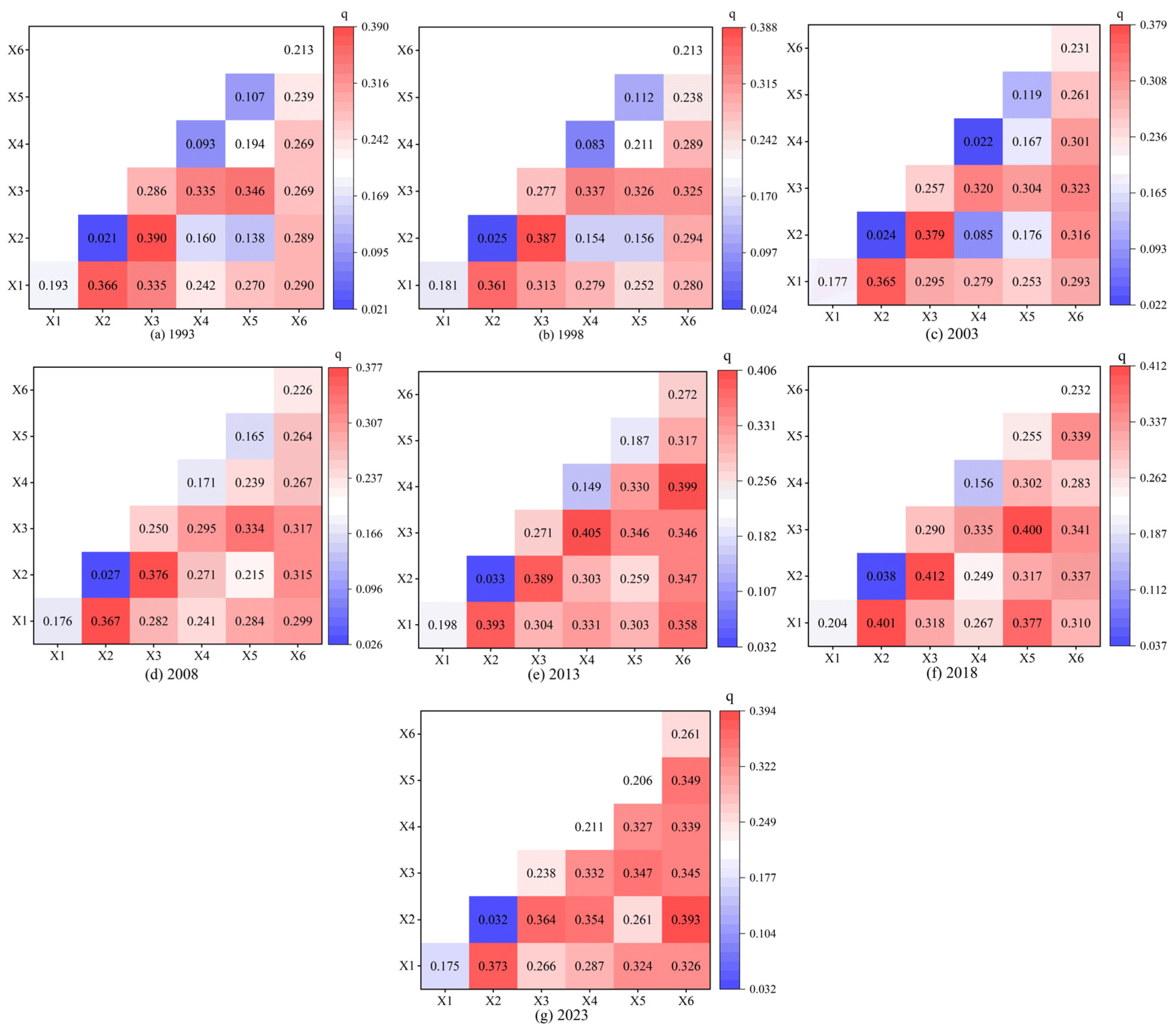
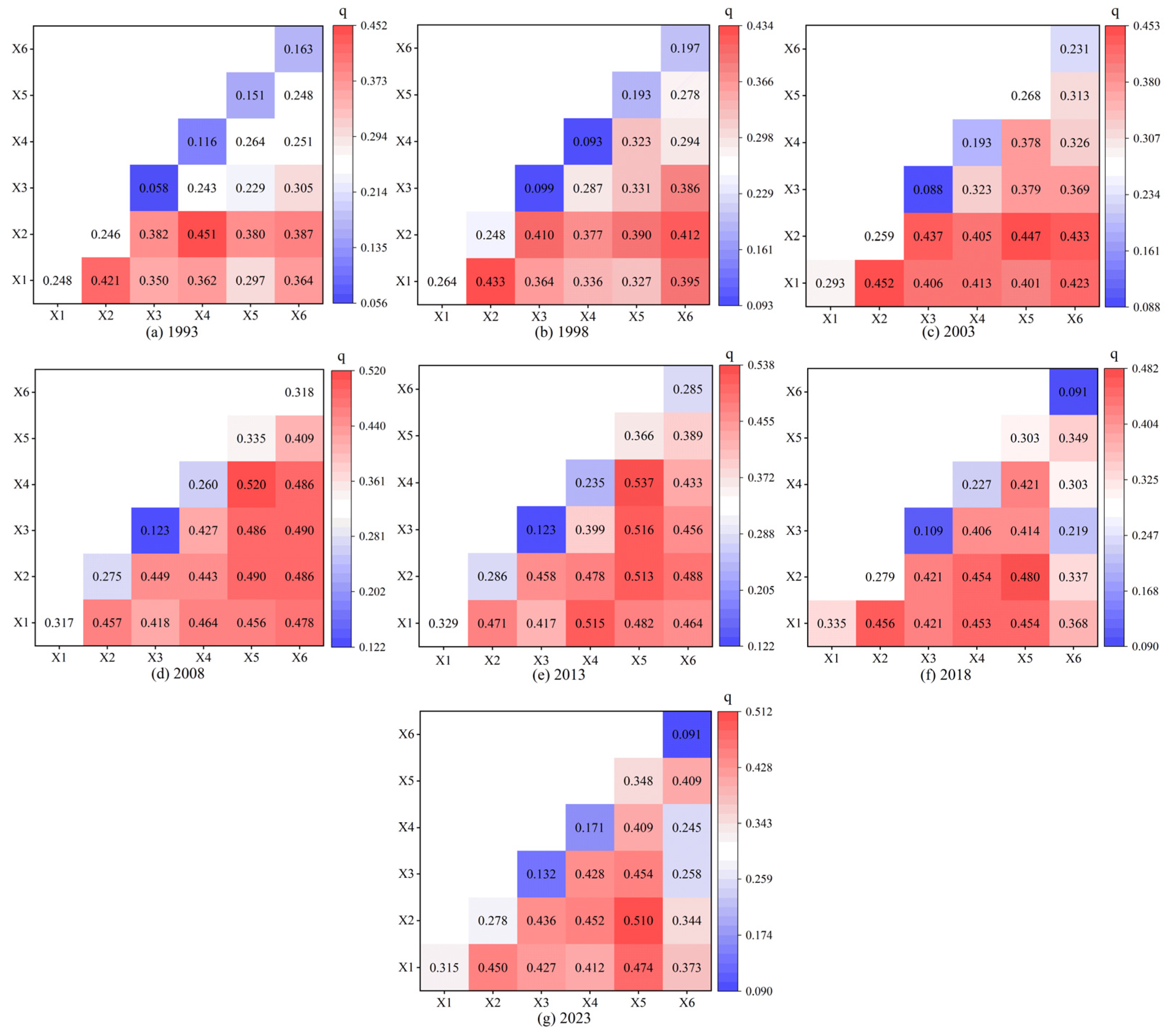
The interactive detection results of edge density (ED) in the upper reaches are presented in Figure 7, demonstrating that a two-factor enhancement effect exists for all driving factors. Among them, the interaction between topographic factors stood out as the most stable and had the highest explanatory power. The interaction q-value between DEM (X1) and slope (X2) remained consistently within the range of 0.361–0.401 over an extended period, while the interaction q-value between slope (X2) and mean annual temperature (X3) also maintained stability, fluctuating between 0.364 and 0.412. Both values were significantly higher than those of the corresponding single factors, suggesting that topographic conditions exhibited stronger spatial associations with the variation in landscape edge density than other individual factors. The interaction between climatic factors ranked second in explanatory power, with the interactive effect between mean annual temperature (X3) and mean annual precipitation (X4) remaining above 0.295 in most years and reaching a high level in 2013 (q = 0.405). The coupling effects between natural and anthropogenic factors intensified over the study period. Specifically, the interaction q-values between GDP (X6) and the other factors, including DEM (X1), slope (X2), mean annual temperature (X3), mean annual precipitation (X4), and nighttime light (X5), rose from 0.239 to 0.290 in 1993 to 0.326–0.393 in 2023, reflecting an increasing contribution of factor interactions to the spatial differentiation of landscape patterns. The spatial differentiation of ED in the upper reaches showed a stronger statistical association with topographic and climatic factors than with the other variables considered. The explanatory power associated with human activity indicators gradually increased over time, although topographic and climatic factors generally maintained higher explanatory power.

The interactive detection results of patch number (NP) in the middle reaches of the YREB are presented in Figure 8. Overall, the driving factors had a significant two-factor enhancement effect, with the interactive explanatory power showing a sustained upward trend over time. Interactions involving topographic and climatic factors remained among the strongest factor combinations throughout the study period. Notably, the q-values for the slope (X2), the mean annual temperature (X3), slope (X2), the mean annual precipitation (X4), and mean annual temperature (X3), the mean annual precipitation (X4) interactions increased from 0.235 to 0.283 in 1993 to 0.407 to 0.451 in 2023, indicating an enhanced joint contribution of topographic and climatic conditions to the spatial differentiation of landscape patterns. These findings indicate that the joint effects of topographic and climatic factors contributed more substantially to the spatial differentiation of landscape patterns than individual factors considered separately. The interaction of natural factors with human activity factors continued to increase. The interactive explanatory power of GDP (X6) with slope (X2) and mean annual temperature (X3) with nighttime light (X5) has increased from the range of 0.193–0.202 in the early period to 0.338–0.422 in recent years. Notably, the interactions between GDP (X6) and slope (X2), as well as between GDP (X6) and nighttime light (X5), have reached high levels in 2023. At the same time, the interaction of the nighttime light (X5) factor with topographic and climatic factors demonstrated the strongest explanatory power during the middle and later stages, with the q-value generally exceeding 0.44. The spatial heterogeneity of NP in the middle reaches exhibited stronger associations with topographic and climatic factors, while the explanatory power of human activity indicators increased progressively over time.

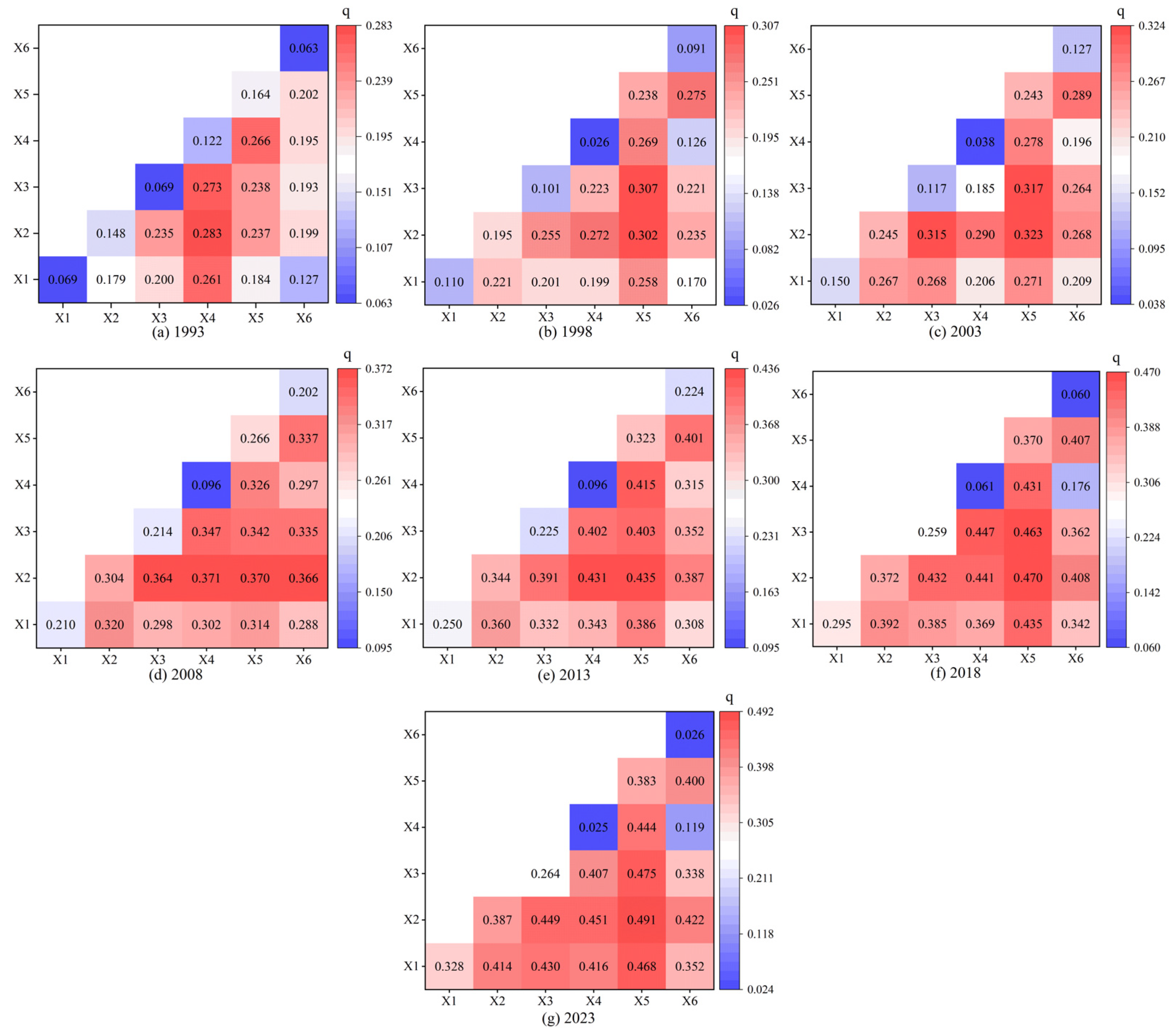
The interactive detection results for SHDI in the lower reaches are presented in Figure 9, where the driving factors generally exhibited a marked two-factor enhancement effect, with an overall level of explanatory power significantly higher than that observed in the upper and middle reaches. Consistently, the interaction between topographic and climatic factors demonstrated high explanatory power. Specifically, the interaction q-values for slope (X2) with mean annual temperature (X3), slope (X2) with mean annual precipitation (X4), and mean annual temperature (X3) with mean annual precipitation (X4) remained stable within the range of 0.40–0.45 across most years, with certain combinations exceeding 0.48 after 2013. This indicated that natural conditions continue to serve as a fundamental constraint on landscape diversity patterns in lower reaches. Increasingly pronounced enhancement features were exhibited by the interaction between human activity factors and natural factors. The interaction q-values for GDP (X6) with slope (X2), mean annual temperature (X3), mean annual precipitation (X4), and nighttime light (X5) generally increased to the range of 0.43–0.49 from 2003 to 2013, and reached a periodic peak during the 2008–2013 interval. Notably, the explanatory power of GDP (X6) with mean annual temperature (X3), mean annual precipitation (X4), and slope (X2), respectively, approached or exceeded 0.48. The interaction between nighttime light (X5) and topographic or climatic factors consistently demonstrated the highest explanatory power. Specifically, the combinations of nighttime light (X5) with mean annual precipitation (X4) and nighttime light (X5) with mean annual temperature (X3) both yielded q-values exceeding 0.50 from 2008 to 2013. The spatial differentiation of SHDI in the lower reaches exhibited stronger associations with human activity indicators, while natural factors continued to provide important environmental context for the observed diversity patterns.

5. Discussion

5.1. Characteristics of Land Use Change and Associated Driving Factors

Existing studies have shown that large-scale regional land use evolution is typically characterized by the coexistence of stability and stage-specific transitions, while evolutionary trajectories among different land use types often exhibit clear differences. The findings of this paper further confirm that, between 1993 and 2023, the study area’s overall land use structure remained generally stable, while its internal composition underwent continuous adjustment. The cultivated land area showed a slow decline. Its spatial distribution displayed a dynamic equilibrium over different periods. This reflected the long-term interplay among food security constraints, land consolidation efforts, and urban expansion [31,32]. In contrast, forest land area stayed relatively stable and increased slightly later. This showed that ecological conservation and restoration policies have gradually yielded cumulative regional effects [33]. The continuous expansion of built-up land represented the most prominent signal of structural transformation, with its evolutionary trajectory exhibiting distinct stage-specific characteristics, transitioning from slow incremental growth in the early phase to rapid expansion during the middle and late stages. This trend was not only consistent with the improvement of regional urbanization levels but also reflected the transformation of the development mode from factor agglomeration to spatial expansion [34].

The evolution of land-use transitions further indicates a shift from natural-resource adjustment to human-dominated spatial restructuring. During the early stage, land-use conversion mainly occurred among cropland, forest land, and grassland, whereas built-up land became the dominant inflow type after 2008 [35], primarily at the expense of cropland. This transition coincided with rapid urbanization and infrastructure development across major urban agglomerations of the YREB. At the same time, national policies, including the Grain for Green Program, the Natural Forest Protection Program, and cultivated-land protection measures, played an important role in regulating land-use transitions. Therefore, the observed land-use changes should be understood as the combined outcome of environmental constraints, socioeconomic development, and policy interventions, which together laid the foundation for subsequent landscape-pattern evolution.

5.2. Landscape Pattern Response and Regional Differences

Land-use restructuring during the past three decades produced distinct landscape responses across the YREB, reflecting substantial regional differences in environmental conditions, development intensity, and policy implementation. Although all three reaches experienced varying degrees of landscape diversification, the underlying processes and ecological implications differed considerably among regions.

The upper reaches maintained a relatively stable landscape structure throughout the study period. This stability was primarily associated with the dominance of mountainous terrain, extensive forest cover, and comparatively low levels of human disturbance. Steep topographic conditions constrained large-scale land conversion and urban expansion, thereby preserving the continuity of ecological land. Meanwhile, long-term ecological restoration initiatives promoted vegetation recovery and enhanced landscape connectivity, further reinforcing the stability of the regional landscape structure [12]. As a result, landscape diversification in the upper reaches mainly reflected gradual adjustments among secondary land-use types within a stable forest-dominated matrix rather than substantial restructuring of the regional landscape. This suggests that increasing landscape diversity can occur without compromising ecological integrity when the dominant ecological framework remains intact.

Compared with the upper reaches, landscape patterns in the middle reaches underwent more pronounced changes over the study period. As a transitional region between the ecologically dominated upper reaches and the highly urbanized lower reaches, the middle reaches were shaped by the combined effects of agricultural production, ecological restoration, and urban expansion. The long-term interaction among these processes continuously reconfigured landscape structure and spatial configuration. Consequently, landscape evolution in the middle reaches reflected a process of ongoing adjustment in which ecological and socioeconomic functions competed for limited land resources. The resulting increase in landscape heterogeneity therefore represented not only changes in land-use composition but also the spatial reorganization of multiple land-use functions [36].

The lower reaches underwent the most intensive landscape restructuring during the study period, resulting in increasingly heterogeneous landscape mosaics and more complex spatial configurations. These processes weakened the dominance of traditional land-use categories and intensified spatial fragmentation and land-use mixing across the landscape. Unlike the upper reaches, where increasing diversity occurred within a relatively stable ecological framework, landscape diversification in the lower reaches was closely associated with increasing fragmentation and declining spatial aggregation. This finding suggests that the ecological implications of increasing diversity are highly context-dependent and cannot be evaluated solely based on compositional indicators [12].

Taken together, the observed regional differences in landscape evolution reflect the combined effects of geographical constraints, socioeconomic development, and policy interventions. The upper reaches remained primarily influenced by ecological processes and conservation policies; the middle reaches represented a transitional landscape shaped by both agricultural and urban dynamics; and the lower reaches experienced extensive human-induced landscape restructuring. These contrasting trajectories demonstrate that similar landscape outcomes may emerge from different combinations of environmental and socioeconomic processes. Compared with other major urban agglomerations in China, such as the Beijing–Tianjin–Hebei region, where landscape changes are closely associated with farmland fragmentation and urban expansion, the YREB exhibits a more complex pattern of landscape evolution due to the coexistence of ecological conservation, agricultural production, and rapid socioeconomic development [37]. Previous studies have shown that the YREB is characterized by pronounced spatial heterogeneity and a clear upper–middle–lower reaches gradient, which distinguishes it from many single urban agglomerations [38]. This unique gradient from ecologically dominated upper reaches to highly urbanized lower reaches highlights the complexity of human–environment interactions within large-scale river-basin systems [39].

More importantly, the results suggest that increasing landscape diversity should not necessarily be interpreted as an improvement in landscape quality. In regions where diversity increases through ecological restoration and balanced land-use composition, it may contribute to greater ecological resilience and functional stability. In contrast, diversity generated by intensive land-use conversion and urban expansion may be accompanied by increasing fragmentation and reduced landscape connectivity. Therefore, assessments of regional landscape sustainability should jointly consider landscape composition and spatial configuration rather than relying on diversity indicators alone. Consistent with previous studies, landscape fragmentation under intensive development does not necessarily lead to a unidirectional decline in ecological functions but may alter trade-offs among ecosystem services through increasing spatial heterogeneity [40].

5.3. Driving Mechanisms and Human–Environment Interactions

The Geodetector analysis provides important insights into the mechanisms underlying landscape evolution in the YREB. Rather than directly modifying landscape structure, natural and socioeconomic factors primarily influence landscape patterns through their effects on land-use transitions. Consequently, changes in land-use composition and spatial allocation constitute the key pathways through which driving factors shape landscape evolution.

Natural environmental conditions provide the fundamental framework for landscape development. Topographic and climatic factors influence vegetation distribution, agricultural suitability, and the spatial allocation of human activities, thereby constraining the distribution and evolution of different land-use types. In regions characterized by complex terrain and strong environmental gradients, these constraints help maintain relatively stable landscape structures and preserve ecological connectivity. This interpretation is consistent with the Geodetector results, which indicate that natural factors maintained relatively strong explanatory power in ecologically dominated regions of the YREB.

In contrast, socioeconomic development has increasingly become a major force driving landscape transformation. Urbanization, economic development, and infrastructure construction have intensified land-use transitions, particularly through the expansion of built-up land and the corresponding reduction in cropland and other land-use categories. These transitions not only alter landscape composition but also reshape spatial configuration by modifying patch size, connectivity, and spatial heterogeneity. As a result, landscape evolution in economically developed areas has become increasingly influenced by human activities and land-development processes, particularly in regions experiencing rapid urbanization and infrastructure expansion.

The interaction analysis further indicates that landscape evolution cannot be attributed to individual factors alone. Natural conditions determine where land conversion is environmentally feasible, whereas socioeconomic forces determine where such conversion is most likely to occur and at what intensity. The strengthening effects of factor interactions suggest that landscape pattern evolution is jointly associated with environmental constraints and anthropogenic activities. Similar interaction effects have been reported in other rapidly developing regions of China, where landscape changes were jointly shaped by topographic suitability and socioeconomic development rather than by individual factors alone [41,42].

Overall, the results support a “natural foundation–human modification” framework for understanding landscape evolution in the YREB. Natural factors provide the environmental context for landscape development, whereas socioeconomic development increasingly shapes the intensity and direction of landscape transformation. These findings highlight the importance of integrating ecological protection, land-use management, and regional development planning to promote long-term landscape sustainability in the YREB.

5.4. Implications, Uncertainties, Limitations and Future Perspectives

The findings highlight the necessity of adopting differentiated land-management strategies across the upper, middle, and lower reaches of the YREB. In the upper reaches, maintaining forest connectivity and ecological integrity should remain a primary management objective, with continued emphasis on ecological conservation and restoration. In the middle reaches, balancing urban expansion, cultivated-land protection, and ecological restoration is essential to prevent excessive landscape fragmentation while maintaining landscape stability. In contrast, the lower reaches face the greatest pressure from urbanization, making it necessary to control urban sprawl, improve land-use efficiency, and strengthen ecological corridor networks to mitigate increasing landscape heterogeneity and enhance regional ecological resilience.

While the results provide valuable insights into the long-term evolution of land-use and landscape patterns, several sources of uncertainty should be acknowledged. This study integrated multiple land-use, climatic, topographic, and socioeconomic datasets spanning 30 years. Although all datasets were standardized to a consistent spatial resolution and coordinate system prior to analysis, uncertainties related to land-use classification accuracy, differences in spatial resolution, and temporal consistency may still influence the calculated landscape metrics and driving-factor analyses. Such uncertainties are particularly relevant in rapidly urbanizing areas and complex transition zones, where land-use boundaries are often dynamic and difficult to classify accurately.

Beyond these data-related uncertainties, the interpretation of driving mechanisms is also constrained by data availability. To ensure long-term temporal consistency and data comparability across the entire YREB from 1993 to 2023, only six representative natural and socioeconomic factors with continuous spatial coverage were incorporated into the Geodetector analysis. Although these variables capture the major environmental and anthropogenic influences on landscape-pattern evolution, other potentially important factors, including population density, transportation accessibility, soil properties, and policy-related variables, were not included because spatially consistent datasets were unavailable throughout the study period. Consequently, the driving mechanisms identified in this study should be regarded as the dominant associations revealed by the selected factors rather than a complete representation of all possible influences.

Methodological considerations should also be taken into account when interpreting the Geodetector results. The q-value reflects the degree of spatial association between explanatory variables and landscape patterns but does not establish causal relationships. Therefore, factors with high explanatory power indicate strong spatial correspondence with landscape variation rather than definitive drivers of change. In addition, the estimated explanatory power may be influenced by factor discretization schemes, spatial-scale selection, and the composition of explanatory variables. Because some environmental and socioeconomic variables exhibit inherent spatial correlations, completely separating their individual contributions remains challenging.

Although the results suggest that landscape evolution is closely associated with land-use transitions driven by natural and socioeconomic factors, the present study did not explicitly quantify the causal pathways linking driving factors, land-use change, and landscape pattern evolution. The proposed relationships are therefore primarily inferred from the combined interpretation of land-use transition analysis and Geodetector results. Future studies integrating structural equation modelling, path analysis, spatial regression, or other causal inference approaches could provide more direct evidence of the mechanisms connecting driving factors, land-use dynamics, and landscape evolution.

The scope of landscape indicators considered in this study also deserves attention. To avoid redundancy among highly correlated metrics and facilitate interpretation of regional driving mechanisms, the analysis focused on three representative indicators (ED, NP, and SHDI) that characterize major dimensions of landscape fragmentation and diversity. While these indicators effectively capture broad patterns of regional landscape evolution, they cannot fully reveal the responses of individual land-use types to environmental and socioeconomic changes. Integrating class-level landscape metrics could therefore provide additional insights into the mechanisms through which specific land-use transitions influence landscape structure and spatial configuration. Similarly, the use of six aggregated land-use categories facilitated consistent long-term analysis across the YREB but may have obscured variations among specific land-use subclasses. Employing more detailed land-use classifications and higher-resolution datasets may also improve understanding of landscape responses to particular land-use transitions.

Future studies should further investigate scale effects and multi-resolution characteristics of landscape evolution to better understand scale-dependent landscape dynamics and support sustainable land-use planning in the YREB.

6. Conclusions

Based on land-use data from seven observation periods between 1993 and 2023, this study integrated land-use transfer analysis, a grid-based framework, landscape metrics, and the Geodetector model to investigate the spatiotemporal evolution of land use and landscape patterns and the spatial heterogeneity of their associated driving factors across the YREB. The results indicate that the overall land-use structure of the YREB remained relatively stable over the past three decades, whereas its internal composition underwent continuous adjustment. Cropland gradually declined, forest land remained largely stable, and built-up land expanded rapidly after 2008, becoming the most prominent land-use transition. These changes were accompanied by increasing landscape fragmentation and diversity, although their manifestations varied considerably among regions. The upper reaches maintained comparatively stable landscape structures under strong environmental constraints; the middle reaches exhibited transitional characteristics shaped by both agricultural and urban processes, whereas the lower reaches experienced the most pronounced landscape reorganization associated with rapid urban expansion. Importantly, increasing landscape diversity should not necessarily be interpreted as an improvement in landscape quality, particularly in highly urbanized areas where greater diversity was frequently associated with increasing fragmentation and reduced connectivity.

These spatially differentiated patterns were closely associated with the combined influences of environmental conditions and socioeconomic development. Natural factors provided the environmental setting and spatial constraints for land-use activities, whereas socioeconomic factors increasingly shaped the pace and spatial configuration of land-use transitions. These land-use transitions constituted an important pathway through which environmental and socioeconomic factors were associated with landscape pattern evolution. Through their joint effects on land-use composition and allocation, these factors were closely associated with the observed evolution of landscape structure and diversity, highlighting the interconnected roles of environmental processes and human activities in regional landscape dynamics.

The marked regional heterogeneity identified in this study underscores the need for differentiated land-management strategies across the YREB. In the upper reaches, strengthening forest conservation and maintaining ecological connectivity should remain key priorities. In the middle reaches, greater emphasis should be placed on coordinating cultivated-land protection, ecological restoration, and urban development to support balanced landscape evolution. In the lower reaches, controlling urban sprawl, improving land-use efficiency, and enhancing ecological corridor networks are essential for strengthening ecological resilience and mitigating landscape fragmentation. Overall, the findings highlight the importance of integrating ecological conservation with sustainable land-use planning to support long-term landscape sustainability and coordinated regional development across the YREB.

References

1. Wan, S.; Ye, L.; Zhao, T.; Lyu, R.; Wang, Y.; Zhang, Z. The effects of landscape patterns on ecosystem services of urban agglomeration in semi-arid area under scenario modeling. Ecol. Indic. 2024, 167, 112610. [Google Scholar] [CrossRef] [Scilit]
2. Wang, J.; Peng, P.; Liu, T.; Wang, J.; Zhang, S.; Niu, P. Revealing the spatiotemporal changes in land use and landscape patterns and their effects on ecosystem services: A case study in the western sichuan urban agglomeration, China. Land 2025, 14, 1012. [Google Scholar] [CrossRef] [Scilit]
3. Gao, Y.; Wang, Z.; Zhang, L.; Chai, J. Spatial identification and multilevel zoning of land use functions improve sustainable regional management: A case study of the yangtze river economic belt, China. Environ. Sci. Pollut. Res. 2023, 30, 27782–27798. [Google Scholar] [CrossRef] [Scilit]
4. Fu, H.; Cai, M.; Jiang, P.; Fei, D.; Liao, C. Spatial multi-objective optimization towards low-carbon transition in the yangtze river economic belt of China. Landsc. Ecol. 2024, 39, 156. [Google Scholar] [CrossRef] [Scilit]
5. Liu, J.; Chen, W.; Ding, H.; Liu, Z.; Xu, M.; Singh, R.P.; Liu, C. Changing characteristics of land cover, landscape pattern and ecosystem services in the bohai rim region of China. Front. Environ. Sci. 2024, 12, 1500045. [Google Scholar] [CrossRef] [Scilit]
6. Che, M.; Yang, F.; Sun, J.; Zhang, C.; Zhang, J. Influence of road network expansion on the landscape ecological risk in the yangtze river delta region over the past two decades. Ecol. Indic. 2023, 156, 111178. [Google Scholar] [CrossRef] [Scilit]
7. Molina Bacca, E.J.; Stevanović, M.; Bodirsky, B.L.; Doelman, J.C.; Parsons Chini, L.; Volkholz, J.; Frieler, K.; Reyer, C.P.O.; Hurtt, G.; Humpenöder, F.; et al. Future land-use pattern projections and their differences within the isimip3b framework. Earth Syst. Dyn. 2025, 16, 753–801. [Google Scholar] [CrossRef] [Scilit]
8. Yao, Y.; Yang, Y. Spatiotemporal effects of landscape structure on the trade-offs and synergies among ecosystem service functions in yangtze river economic belt, China. Sci. Rep. 2025, 15, 15767. [Google Scholar] [CrossRef] [Scilit]
9. Zhou, J.; Chen, W.; Cai, Y.; Meng, Y.; Wang, Y.; Liu, Q.; Luo, S.; Peng, J. Effects of landscape pattern changes on ecosystem services: A case study of ruoergai plateau. Sci. Rep. 2025, 15, 45753. [Google Scholar] [CrossRef] [Scilit]
10. Lin, X.; Zhang, Y.; Zou, C.; Chen, X.; Wu, T.; Zhou, W.; Ouyang, Z. How landscape structure influences water-related ecosystem service flows. Landsc. Ecol. 2025, 40, 121. [Google Scholar] [CrossRef] [Scilit]
11. Dong, S.; An, H.; Dong, S. Assessing driving factors and future trends of ecological vulnerability in the upper reaches of the yangtze river. Geomat. Nat. Hazards Risk 2026, 17, 2615777. [Google Scholar] [CrossRef] [Scilit]
12. Kou, X.; Zhao, J.; Sang, W. Impact of typical land use expansion induced by ecological restoration and protection projects on landscape patterns. Land 2024, 13, 1513. [Google Scholar] [CrossRef] [Scilit]
13. Gong, X.; Liu, S.; Ye, W.; Liu, L. Decoupling of industrial water consumption and economic expansion in the yangtze river economic belt: A comparative analysis across three five-year plans. Sci. Rep. 2025, 15, 21186. [Google Scholar] [CrossRef] [Scilit]
14. Yang, S.; Song, W.; Li, Y.; Hu, S. How do urban network externalities affect regional economic growth? Evidence and heterogeneity analysis from china’s yangtze river economic belt. Urban Sci. 2026, 10, 163. [Google Scholar] [CrossRef] [Scilit]
15. Yang, F.; Yang, L.; Fang, Q.; Yao, X. Impact of landscape pattern on habitat quality in the yangtze river economic belt from 2000 to 2030. Ecol. Indic. 2024, 166, 112480. [Google Scholar] [CrossRef] [Scilit]
16. Yang, J.; Huang, X. The 30 m annual land cover dataset and its dynamics in china from 1990 to 2019. Earth Syst. Sci. Data 2021, 13, 3907–3925. [Google Scholar] [CrossRef] [Scilit]
17. Zheng, L.; Wang, Y.; Li, J. Quantifying the spatial impact of landscape fragmentation on habitat quality: A multi-temporal dimensional comparison between the yangtze river economic belt and yellow river basin of China. Land Use Policy 2023, 125, 106463. [Google Scholar] [CrossRef] [Scilit]
18. He, Y.; Zhao, Z.; Mei, Z.; Bai, H. Spatiotemporal evolution of land use and habitat quality in the three-river source region. Sci. Rep. 2025, 15, 37214. [Google Scholar] [CrossRef] [Scilit]
19. Nguyen, B.Q.; Tran, T.-N.-D.; Grodzka-Łukaszewska, M.; Sinicyn, G.; Lakshmi, V. Assessment of urbanization-induced land-use change and its impact on temperature, evaporation, and humidity in central vietnam. Water 2022, 14, 3367. [Google Scholar] [CrossRef] [Scilit]
20. Li, Z.; Xu, Z.; Chen, Y.; Gu, S.; Li, C. Impacts of landscape patterns on habitat quality in coal resource-exhausted cities: Spatial–temporal dynamics and non-stationary scale effects. Environ. Monit. Assess. 2025, 197, 297. [Google Scholar] [CrossRef] [Scilit]
21. Yaermaimaiti, A.; Li, X.; Ge, X.; Liu, C. Analysis of landscape pattern and ecological risk change characteristics in bosten lake basin based on optimal scale. Ecol. Indic. 2024, 163, 112120. [Google Scholar] [CrossRef] [Scilit]
22. Ran, P.; Hu, S.; Frazier, A.E.; Qu, S.; Yu, D.; Tong, L. Exploring changes in landscape ecological risk in the yangtze river economic belt from a spatiotemporal perspective. Ecol. Indic. 2022, 137, 108744. [Google Scholar] [CrossRef] [Scilit]
23. Zhang, X.; Zhang, S.; Zhang, X.; Liu, J.; Xue, X. Spatial and temporal evolution of landscape ecological security and its influencing factors in the yangtze river economic belt from the perspective of production-living-ecological space in the past 40 years. Chin. J. Eco-Agric. 2023, 31, 1539–1552. [Google Scholar] [CrossRef]
24. Jia, L.; Yu, K.; Li, Z.; Li, P.; Xu, G.; Li, B. Probability evaluation of the impact of landscape pattern on ecosystem service value in the yangtze river economic belt. Trans. Chin. Soc. Agric. Eng. 2023, 39, 217–227. [Google Scholar] [CrossRef]
25. Ma, X.; Wu, H.; Qin, B.; Wang, L. Spatiotemporal change of landscape pattern and its eco-environmental response in the yangtze river economic belt. Geogr. Sci. 2022, 42, 1706–1716. [Google Scholar] [CrossRef]
26. Schumaker, N.H. A rapid assessment methodology for quantifying and visualizing functional landscape connectivity. Front. Conserv. Sci. 2024, 5, 1412888. [Google Scholar] [CrossRef] [Scilit]
27. Benitez, L.M.; Parr, C.L.; Sankaran, M.; Ryan, C.M. Fragmentation in patchy ecosystems: A call for a functional approach. Trends Ecol. Evol. 2025, 40, 27–36. [Google Scholar] [CrossRef] [Scilit]
28. Wang, J.; Xu, C.D. Geodetector: Principle and prospective. Acta Geogr. Sin. 2017, 72, 116–134. [Google Scholar] [CrossRef]
29. Ke, S.; Cui, H.; Lu, X. Geodetector analysis of spatio-temporal patterns and driving mechanisms of farmland spatial transition within 897 counties in the yangtze river economic belt, China. Humanit. Soc. Sci. Commun. 2025, 12, 923. [Google Scholar] [CrossRef] [Scilit]
30. Li, Y.; Fan, W.; Yuan, X.; Li, J. Spatial distribution characteristics and influencing factors of traditional villages based on geodetector: Jiarong tibetan in western sichuan, China. Sci. Rep. 2024, 14, 11700. [Google Scholar] [CrossRef] [Scilit]
31. Zhong, Y.; Lin, A.; He, L.; Zhou, Z.; Yuan, M. Spatiotemporal dynamics and driving forces of urban land-use expansion: A case study of the yangtze river economic belt, China. Remote Sens. 2020, 12, 287. [Google Scholar] [CrossRef] [Scilit]
32. Xia, J.; Hong, M.; Wei, W. Changes and driving forces of urban–agricultural–ecological space in the yangtze river economic belt from 2000 to 2020. Land 2023, 12, 1014. [Google Scholar] [CrossRef] [Scilit]
33. Dong, B.; Huang, T.; Tang, T.; Huang, D.; Tang, C. Impact of multi-scenario land-use changes on habitat quality evolution in the yangtze river economic belt. Front. Environ. Sci. 2025, 12, 1516703. [Google Scholar] [CrossRef] [Scilit]
34. Jiang, X.; Chu, X.; Yang, X.; Jiang, P.; Zhu, J.A.; Cai, Z.; Yu, S. Spatiotemporal dynamics of land use carbon balance and its response to urbanization: A case of the yangtze river economic belt. Land 2024, 14, 41. [Google Scholar] [CrossRef] [Scilit]
35. Zeng, X.; Huang, Y.; Xie, H.; Ma, Q.; Li, J. Impacts of land use and land cover change on the landscape pattern and ecosystem services in the poyang lake basin, China. Landsc. Ecol. 2024, 39, 183. [Google Scholar] [CrossRef] [Scilit]
36. Wang, Q.; Bai, X. Spatiotemporal characteristics and driving mechanisms of land-use transitions and landscape patterns in response to ecological restoration projects: A case study of mountainous areas in guizhou, southwest China. Ecol. Inform. 2024, 82, 102748. [Google Scholar] [CrossRef] [Scilit]
37. Xu, M.; Niu, L.; Wang, X.; Zhang, Z. Evolution of farmland landscape fragmentation and its driving factors in the beijing-tianjin-hebei region. J. Clean. Prod. 2023, 418, 138031. [Google Scholar] [CrossRef] [Scilit]
38. Bian, H.; Gao, J.; Wu, J.; Sun, X.; Du, Y. Hierarchical analysis of landscape urbanization and its impacts on regional sustainability: A case study of the yangtze river economic belt of China. J. Clean. Prod. 2021, 279, 123267. [Google Scholar] [CrossRef] [Scilit]
39. Wei, W.; Wang, N.; Yin, L.; Guo, S.; Bo, L. Spatio-temporal evolution characteristics and driving mechanisms of urban–agricultural–ecological space in ecologically fragile areas: A case study of the upper reaches of the yangtze river economic belt, China. Land Use Policy 2024, 145, 107282. [Google Scholar] [CrossRef] [Scilit]
40. Qi, Y.; Shen, P.; Ren, S.; Chen, T.; Hu, Y. Coupling effect of landscape patterns on the spatial and temporal distribution of ecosystem services: A case study in harbin city, northeast China. Sci. Rep. 2025, 15, 4606. [Google Scholar] [CrossRef] [Scilit]
41. Gan, L.; Halik, Ü.; Shi, L.; Ru, J.; Wei, Z.; Li, J.; Welp, M. Integrating multi-source data to explore spatiotemporal dynamics and future scenarios of arid urban agglomerations: A geodetector–plus modelling framework for sustainable land use planning. Remote Sens. 2025, 17, 1851. [Google Scholar] [CrossRef] [Scilit]
42. Zhang, C.; Wang, Z.; Wang, Q.; Yang, C. Interaction of population density and slope will exacerbate spatiotemporal changes in land use and landscape patterns in mountain city. Sci. Rep. 2025, 15, 3168. [Google Scholar] [CrossRef] [Scilit]
Figure 1. Study area location map.
Land 15 01583 g001
Figure 2. Proportion of land use types in the YREB. Note: Grey dots indicate values scaled by 10×.
Land 15 01583 g002
Figure 3. Spatial distribution of land use in the YREB. (a) 1993, (b) 1998, (c) 2003, (d) 2008, (e) 2013, (f) 2018, (g) 2023.
Land 15 01583 g003
Figure 4. Sankey diagram of land use transfer in the YREB.
Land 15 01583 g004
Figure 5. Evolution of landscape-level metrics across the upper, middle, and lower reaches of the Yangtze River Economic Belt, 1993–2023. Note: NP = Number of Patches; PD = Patch Density (patches/ha); ED = Edge Density (m/ha); LPI = Largest Patch Index (%); AI = Aggregation Index (%); CONTAG = Contagion Index (%); SHEI = Shannon’s Evenness Index; SHDI = Shannon’s Diversity Index. (a) NP, (b) PD, (c) ED, (d) LPI, (e) AI, (f) CONTAG, (g) SHEI, and (h) SHDI.
Land 15 01583 g005
Figure 6. Evolution of class-level landscape metrics for major land-use types in the Yangtze River Economic Belt (1993–2023). Note: PLAND = Percentage of Landscape (%); NP = Number of Patches; ED = Edge Density (m/ha); LSI = Landscape Shape Index; COHESION = Patch Cohesion Index; AI = Aggregation Index (%). (a) 1993, (b) 2003, (c) 2013, and (d) 2023.
Land 15 01583 g006
Figure 7. Interactive effects on Edge Density (ED) in the upper reaches.
Land 15 01583 g007
Figure 8. Interactive effects on Number of Patches (NP) in the middle reaches.
Land 15 01583 g008
Figure 9. Interactive effects on Shannon’s Diversity Index (SHDI) in the lower reaches.
Land 15 01583 g009