Article

Crossing the Boundary: A New Perspective Unmasking the Differential Evolution and Divergent Drivers of Ecosystem Service Trade-Offs

1
School of Geography and Environment, Jiangxi Normal University, Nanchang 330022, China
2
China Railway Water Conservancy and Hydropower Planning and Design Group Co., Ltd., Nanchang 330022, China
3
Key Laboratory of Poyang Lake Wetland and Watershed Research Ministry of Education, Jiangxi Normal University, Nanchang 330022, China
4
Jiangxi Provincial Key Laboratory of Natural Disaster Monitoring, Early Warning and Assessment, Jiangxi Normal University, Nanchang 330022, China
*
Author to whom correspondence should be addressed.
Land 2026, 15(9), 1551; https://doi.org/10.3390/land15091551
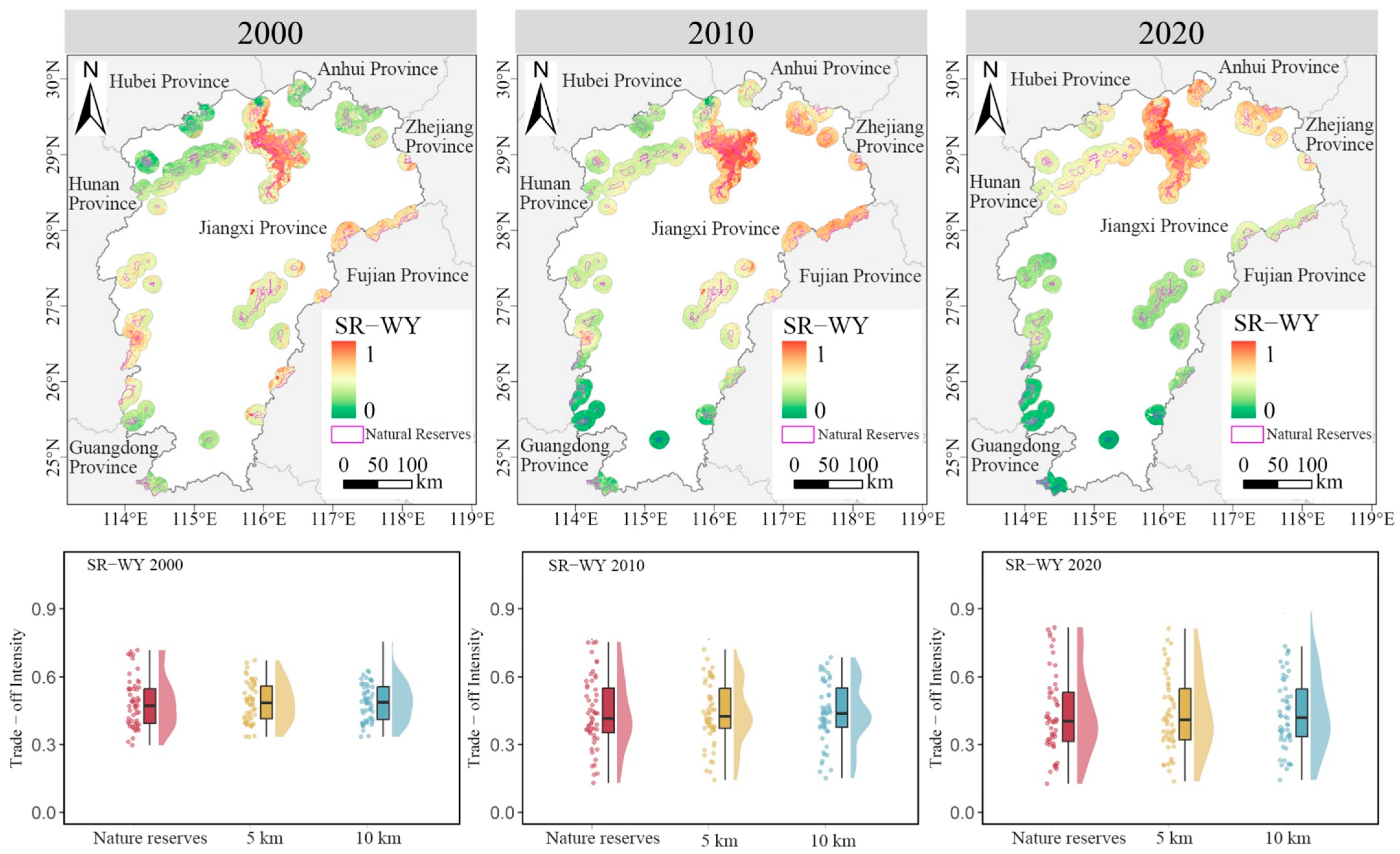
Submission received: 29 July 2026 / Revised: 20 August 2026 / Accepted: 21 August 2026 / Published: 24 August 2026

Abstract

Nature reserves (NRs) sustain biodiversity and multiple ecosystem services (ESs), yet assessments commonly stop at administrative boundaries and seldom examine how service relationships and associated factors vary across surrounding landscape gradients. We assessed carbon storage (CS), habitat quality (HQ), soil retention (SR), and water yield (WY) in 54 NRs in Jiangxi Province, China, and nested 5 and 10 km surrounding zones for 2000, 2010, and 2020. The InVEST model, a comprehensive ecosystem service index (CESI), correlation analysis, RMSE, and GeoDetector were used to characterize service dynamics, trade-offs/synergies, and spatial associations. CS and HQ increased slightly, whereas SR and WY rose until 2010 and subsequently declined. Mean CESI decreased outward from NR interiors (0.53) to the 5 km (0.50) and 10 km zones (0.49), although WY was higher outside NRs in 2020. CS–HQ and SR–WY were predominantly synergistic, while HQ–SR showed the strongest trade-off. Dominant associated factors and their interactions varied among services and spatial zones. These findings reveal context-dependent cross-boundary differentiation in ecosystem-service patterns, supporting coordinated management of NRs and their surrounding landscapes and service-specific conservation priorities.

1. Introduction

Nature reserves (NRs) serve as critical spatial carriers for conserving natural resources and the environment, playing an indispensable role in maintaining biodiversity, mitigating climate change, and enhancing ecosystem services (ESs) [1,2]. The Kunming–Montreal Global Biodiversity Framework calls for at least 30% of terrestrial, inland-water, coastal, and marine areas to be effectively conserved and managed by 2030. Importantly, Target 3 emphasizes not only protected-area coverage but also ecological representativeness, connectivity, conservation outcomes, and integration into wider landscapes [3]. This policy shift redirects attention from how much land is designated for protection to whether protected areas generate sustained ecological benefits under climate change and increasing human pressure [4,5,6,7,8].
ESs provide an outcome-oriented basis for evaluating these benefits because they connect ecosystem condition with functions that support both biodiversity and human well-being. Nature reserves may contribute simultaneously to carbon storage, soil retention, water regulation, and habitat maintenance [6,9,10,11]. However, these functions are not independent. Changes in vegetation, land use, climate, or management may improve several services simultaneously, but may also enhance one service at the expense of others. Consequently, evaluating only a single service—or aggregating multiple services into one composite value—may conceal important trade-offs and synergies [12,13,14]. A more informative evaluation should therefore consider both the level of service provision and the relationships among services.
Protected-area effectiveness assessments have progressively moved beyond descriptions of temporal change within individual reserves. Recent studies have compared ESs inside reserves with those in adjacent or statistically matched, unprotected areas. At the national scale, Liu et al. [15] assessed multiple ESs across 75 Chinese NRs and examined relationships among their effectiveness indices and associated environmental factors. Zhao et al. [16] compared biodiversity and ES outcomes inside and outside protected areas in the Three-River Source Region. Yu et al. [17] further applied statistical matching to estimate the contribution of Chinese protected areas to multiple ESs. At the global scale, Li et al. [18] combined cross-boundary surrounding-zone gradients with matched comparisons and causal inference to examine how effectively protected areas resisted habitat loss. These studies demonstrate that comparisons between protected and surrounding landscapes are already an important direction in conservation-effectiveness research.
Despite these advances, existing research has rarely integrated spatial gradients, multi-service relationships, and their context-dependent correlates within a unified analytical framework. Large-scale ES assessments typically compare average service levels or effectiveness indices between protected and unprotected areas, while representing surrounding landscapes with a single comparison zone [2,19,20,21,22]. Such designs provide limited insight into how ecological patterns vary with increasing distance from reserve boundaries [5,23]. Cross-boundary and surrounding-zone-gradient studies have also focused primarily on habitat loss, vegetation condition, human pressure, or individual ESs, with comparatively little attention to the relational structure of multiple services. Similarly, analyses of ES trade-offs and synergies are commonly conducted at the scale of entire reserves or broader administrative regions, leaving potential differences between reserve interiors and surrounding landscapes insufficiently explored. The key question is, therefore, not only whether ES values differ across reserve boundaries. It is also how individual services and their relationships vary between reserve interiors and surrounding landscapes. Their associated environmental and anthropogenic correlates may also differ across these spatial contexts.
Analyzing ES relationships within and beyond reserve boundaries is necessary because administrative boundaries are discrete, whereas ecological processes and human pressures operate continuously across space. Hydrological flows, species movement, climate forcing, land-use change, and displaced development pressure can connect reserve interiors with surrounding landscapes [15]. Higher ES values inside a reserve may therefore coexist with declining services, intensified trade-offs, or increased human pressure immediately outside its boundary. Conversely, favorable conditions in surrounding landscapes may support ecological functions within the reserve. Comparing ES relationships across reserve interiors and distance-defined surrounding zones can reveal these spatial differences and provide a stronger basis for coordinated conservation beyond administrative boundaries [22,24]. Because reserve designation is spatially non-random, however, adjacent surrounding zones should be interpreted as surrounding landscape contexts rather than as strict counterfactual control areas unless environmental differences are controlled statistically.
Jiangxi Province provides an appropriate setting for such an assessment because its 54 NRs encompass national and provincial administrative levels and four conservation types, including forest ecosystems, wildlife, wild plants, and inland wetlands [24]. These reserves are embedded in landscapes with substantial climatic, topographic, ecological, and human-pressure gradients. This study therefore evaluates carbon storage, habitat quality, soil retention, water yield, and their comprehensive performance within NRs and in 5 km and 10 km surrounding zones in 2000, 2010, and 2020. It addresses three questions: (1) How do individual and comprehensive ES performance vary over time and among reserve interiors, surrounding zones, administrative levels, and conservation types? (2) Do the direction and intensity of ES trade-offs and synergies change across reserve boundaries? (3) Do the dominant environmental and anthropogenic factors associated with ES patterns differ among reserve interiors and surrounding landscapes? By integrating temporal change, reserve characteristics, distance from boundaries, ES relationships, and associated drivers, this study extends existing protected–unprotected comparisons from determining whether service levels differ to explaining how multiple ESs and their relationships vary across reserve boundaries.

2. Materials and Methods

2.1. Study Area

Jiangxi Province (24°29′14″–30°04′43″ N, 113°34′18″–118°28′56″ E) contains 54 NRs listed in the 2017 National Directory of Nature Reserves, including 16 national reserves (254,677.8 ha) and 38 provincial reserves (386,974.2 ha) (Supplementary Table S1). The reserves comprise 35 forest ecosystem reserves, 16 wildlife reserves, two wild-plant reserves, and one inland-wetland reserve. Establishment-year records show that 34 reserves (63%) were established by 2000 and 42 (78%) by 2005; 20 were established after 2000.
To strengthen conservation capacity and biodiversity protection, Jiangxi Province has introduced a series of monitoring and management plans. NRs in the province play a vital role in safeguarding biodiversity and delivering ESs; however, their ecological effectiveness is facing increasing challenges under rapid socioeconomic development and intensive land-use change. In response, the provincial government released two policy frameworks: the “Medium- and Long-term Biodiversity Monitoring Plan for NRs in Jiangxi Province (2021–2035)” and the “Implementation Plan for Biodiversity Monitoring in NRs (2021–2025)”. These plans aim to ensure effective protection of biodiversity and representative ecosystems by 2025, and to substantially enhance reserve management and ecological product supply capacity by 2035.
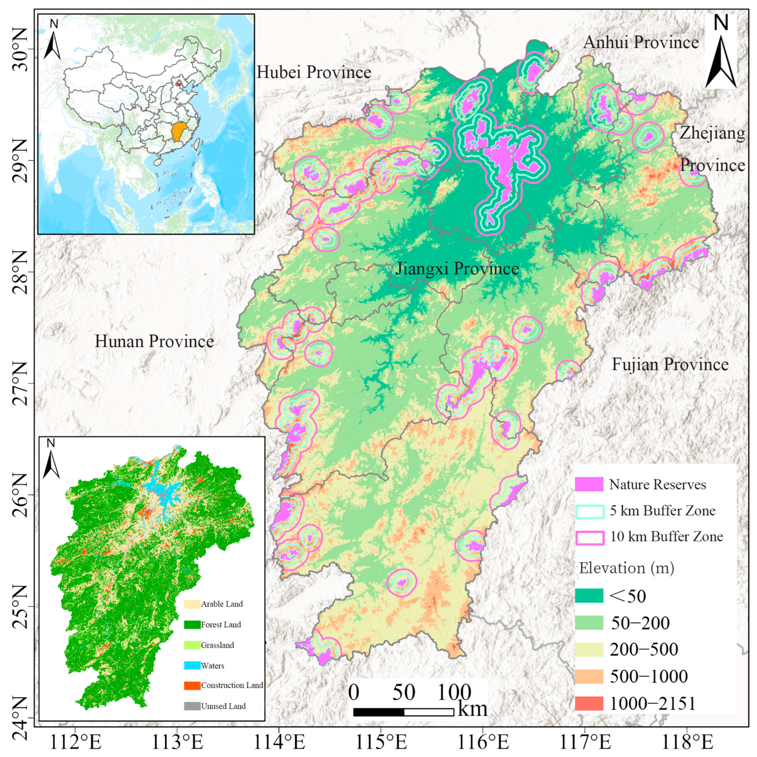
We constructed nested 5 km and 10 km distance envelopes around each reserve to examine whether ES patterns changed with proximity to reserve boundaries (Figure 1 and Figure S1). These fixed distances provide comparable diagnostic scales across a heterogeneous reserve system and are consistent with recent protected-area studies that evaluate adjacent landscapes using multi-distance surrounding zones [18]. The two zones are not ecological thresholds and were not treated as independent controls. Surrounding zones of nearby reserves can overlap with one another and with other protected areas; analyses were conducted reserve by reserve, and these overlaps were retained. Accordingly, the zones represent surrounding landscape contexts, not strictly unprotected areas.

2.2. Assessment of ESs

This study employs the InVEST model to analyze spatiotemporal changes in ESs within NRs, constructs a comprehensive ecosystem service index, and evaluates the conservation effectiveness of NRs [25].

2.2.1. Water Yield

The InVEST model is the most widely used tool for assessing WY services [26]. The WY module evaluates annual WY based on precipitation, potential evapotranspiration, vegetation type, soil depth, and plant-available water content. The calculation formula is as follows:
W Y x j = 1 A E T x P x × P x
where W Y x j is the annual W Y of grid cell x ; A E T x is the annual actual evapotranspiration of grid cell x (mm); P x is the annual precipitation of grid cell x (mm).

2.2.2. Soil Retention

SR service refers to the capacity of ecosystems to store soil nutrients and prevent their loss through erosion processes. This study employs the SR module of the InVEST model to quantify SR in Jiangxi Province’s nature reserves, calculated as the difference between potential soil erosion and actual soil erosion [27]. The formula is expressed as follows:
S R = S L P S L
S L P = R × K × L S
S L = R × K × L S × C × P
In the formula, S R is the soil conservation amount; S L P is the potential soil erosion amount; S L is the actual soil erosion amount; R is the rainfall erosivity factor; K is the soil erodibility factor; L S is the slope length and steepness factor; C is the cover and management factor; and P is the support practice factor.

2.2.3. Carbon Storage

The InVEST model demonstrates strong reliability in estimating CS [27]. Terrestrial ecosystems such as grasslands, wetlands, and forests absorb and sequester atmospheric CO2 through photosynthesis in soil, vegetation, and litter layers, thereby providing climate regulation services. Consequently, the primary carbon pools within a land parcel depend on four fundamental carbon pools: above ground biomass, below ground biomass, soil, and dead organic matter. The calculation formula for CS is expressed as follows:
C t a t a l = C a b a v e + C b e l o w + C s o i l + C d e a d
In the above formula, C t a t a l represents the total of CS; C a b a v e represents the CS above ground; C b e l o w represents the CS below ground; C s o i l represents the CS of soil; C d e a d represents the CS of dead organic. The carbon density refers to the research results of similar study areas [28].

2.2.4. Habitat Quality

HQ reflects the potential of ecosystems to provide necessary conditions for species survival and reproduction, serving as a critical indicator for biodiversity conservation. This module integrates land type sensitivity and the intensity of external threats, which are dominated by human activities, to analyze the distribution of HQ responses to threat sources across different land use types [29]. The formula is expressed as follows:
H Q x j = H j 1 D x j z D x j z + K z
D x j = r = 1 R y = 1 Y r w r r = 1 R w r R y i r x y β x S j r
In the above formula, H Q x j denotes the HQ of grid x in land use type j ; H j represents the habitat suitability of grid x in land use type j ; D x j indicates the habitat degradation degree of grid x in land use type j ; K is the half-saturation constant, typically set to half of the maximum degradation value; z denotes the default normalization constant of the model; R refers to the number of threat factors; y represents the total number of grids containing threat factor r ; Y r is the number of grids occupied by threat factor r ; w r indicates the weight assigned to threat factor r ; R y reflects the value of threat factor y in a given grid (binary values: 0 or 1); i r x y describes the stress intensity imposed on habitat grid x by the threat value R y from grid y ; β x represents the accessibility level of threat factors to grid x (ranging from 0 to 1); S j r signifies the sensitivity of land use type to threat factor r (ranging from 0 to 1).

2.2.5. Comprehensive Ecosystem Service Index (CESI)

The CESI summarizes the four normalized indicators on a common 0–1 scale. We first applied min–max normalization separately to CS, HQ, SR, and WY, and then assigned each service an equal weight of 0.25 before aggregation [30,31]. Equal weighting was selected as a transparent baseline because no defensible stakeholder-derived, policy-derived, or empirical priority weights were available across all 54 reserves and four reserve types. It prevents any service from being privileged by an unverified value judgment, but it does not imply that the services are ecologically equivalent. Composite-index results can vary with normalization, weighting, and aggregation choices, so continuous individual-service results remain primary.
y i j = x i j x m i n x m a x x m i n
In the formula, y i j represents the standardized value of ecosystem service i ; x i j denotes the original data value of ecosystem service i ; x m a x and x m i n refer to the maximum and minimum values, respectively, of the state index j for the ecosystem service.
C E S I = i = 1 n e s i
In the formula, CESI denotes the comprehensive ecosystem service index, while e s i represents the standardized value of the i -th category of ecosystem service.
Based on the computed results, the CESI in this study was categorized into three distinct classes: Class I was defined as the high-benefit zone (CESI > 0.6); Class II as the medium-benefit zone (0.4 < CESI ≤ 0.6); and Class III as the low-benefit zone (CESI ≤ 0.4). A higher CESI value is indicative of greater provision of ESs and improved ecological benefits.

2.3. Trade-Off and Synergistic Evaluation

2.3.1. Pearson Correlation Analysis

Based on the Pearson correlation coefficient, we calculated the trade-offs and synergistic relationships among the overall ESs for 2000, 2010, and 2020. A positive correlation coefficient indicates a synergistic relationship, whereas a negative value suggests a trade-off relationship. The formula is given as follows:
r = i = 1 n E S 1 i j E S ¯ 1 i j E S 2 i j E S ¯ 2 i j i = 1 n ( E S 1 i j E S ¯ 1 i j ) 2 i = 1 n ( E S 1 i j E S ¯ 1 i j ) 2
In the formula, E S 1 and E S 2 represent two distinct ESs, and r denotes the correlation coefficient between E S 1 and E S 2 . The variable n refers to the time series of the raster data, while i and j correspond to the row and column indices of the raster cells, respectively.

2.3.2. Root Mean Square Error (RMSE)

Correlation analysis is a widely used method for assessing trade-offs among ESs; however, it does not quantify the strength of trade-offs between two or more ESs. The Root Mean Square Error (RMSE), as a straightforward and effective metric, can be applied to quantify the intensity of trade-offs among multiple ESs. A higher RMSE value indicates a stronger trade-off intensity. The calculation formula is given as follows:
R M S E = 1 n 1 i = 1 n ( E S E S ¯ ) 2
where RMSE represents the trade-off intensity, E S denotes the ecosystem service value, n is the number of ESs considered, and E S ¯ refers to the expected value of the n ESs.
Based on the definitions of trade-offs and synergies and the results of Pearson correlation analysis, the relationships between ESs were classified into five categories: (a) Strong synergistic relationship: r > 0, with a significance level of p < 0.05; (b) Weak synergistic relationship: r > 0, p > 0.05; (c) Strong trade-off relationship: r < 0, p < 0.05; (d) Weak trade-off relationship: r < 0, p > 0.05; (e) No correlation: r = 0. The same classification procedure was applied to both the 5 km and 10 km surrounding zones. The trade-off intensity between ESs was quantitatively evaluated using RMSE, where a higher RMSE corresponds to a stronger trade-off. The results of trade-off intensity were further categorized into two groups: high trade-off (RMSE ≥ 0.5) and low trade-off (RMSE < 0.5) [32].

2.4. Geographical Detector

GeoDetector was used to quantify spatially stratified heterogeneity and the explanatory power of service-specific candidate factors and their pairwise interactions. The analysis was conducted once, using three-year mean ES values as the dependent variables and predominantly 2020 covariates as the explanatory context. Direct InVEST inputs and close proxies were screened separately for each service before external-factor interpretation (Section 3.3). GeoDetector q values indicate spatial co-distribution and explanatory power, not independent causal effects. The equation is:
q = 1 i = 1 L N i σ i 2 N σ 2
where q denotes the explanatory power of the driving factor; i refers to the stratification of the independent or dependent variable; N i represents the number of units in the i -th stratum; N is the total number of units across the study area; σ i 2 is the variance of the dependent variable within the i -th stratum; and σ 2 denotes the overall variance of the dependent variable in the entire region. A higher q value indicates a stronger explanatory power of the factor regarding the spatial distribution of ESs [26].

2.5. Data

We integrated meteorological, topographic, vegetation, soil, land-use, and human-activity datasets (Table 1). Land use and meteorological inputs were available for 2000, 2010, and 2020. All layers were aligned to a 30 m analysis grid. Categorical layers were resampled with nearest-neighbor assignment and continuous layers with bilinear interpolation. Resampling 1 km data to 30 m ensured grid alignment only; it did not create new fine-scale information.

3. Results

3.1. Spatial and Temporal Patterns of Ecosystem Services in NRs and Surrounding Zones

3.1.1. Individual Ecosystem Service Indicators

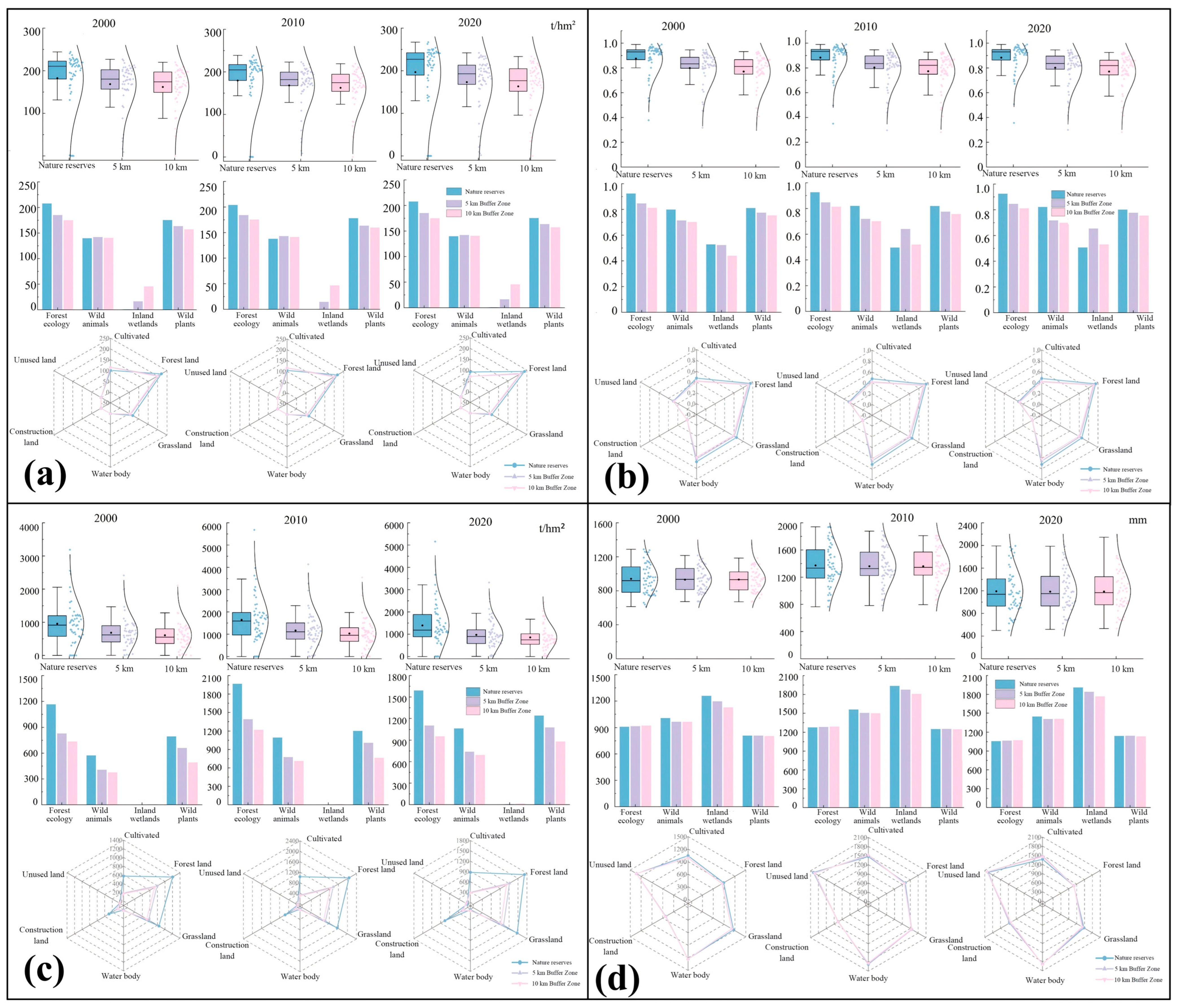
Across the study area, total CS decreased slightly from 966 million t in 2000 to 954 million t in 2010. It then increased to 1.037 billion t in 2020, representing a net increase of 7.35% over the study period (Figure 2a). Mean HQ remained relatively stable, increasing from 0.875 to 0.883. The net increase was 0.0076, or 0.91% (Figure 2b). SR increased sharply from 955.18 t/ha in 2000 to 1,643.46 t/ha in 2010, an increase of 72.06%. It subsequently decreased by 15.26% to 1392.59 t/ha in 2020 (Figure 2c). Annual WY showed a similar pattern. It increased from 940.98 mm in 2000 to 1373.10 mm in 2010 and then decreased to 1191.40 mm in 2020. These changes corresponded to an increase of 45.92% followed by a decrease of 13.23% (Figure 2d). Overall, CS and HQ showed only small net increases, whereas SR and WY varied more strongly and did not follow a consistent upward or downward trend.
Similar temporal patterns of SR and WY were observed within NRs and in both surrounding zones. Both services increased from 2000 to 2010 and decreased thereafter, while HQ remained relatively stable. CS increased gradually in the 5 km zone. In the 10 km zone, it initially decreased and then recovered. CS, HQ, and SR were generally higher within NRs than in the surrounding zones. In contrast, WY was higher in both surrounding zones than within NRs in 2020. Areas with greater forest cover also tended to have higher CS, HQ, and SR values (Figure 2). These differences should be interpreted as spatial contrasts rather than direct management effects because the analysis did not control for pre-existing differences in topography, ecosystem type, and land-cover composition between reserve interiors and surrounding zones.
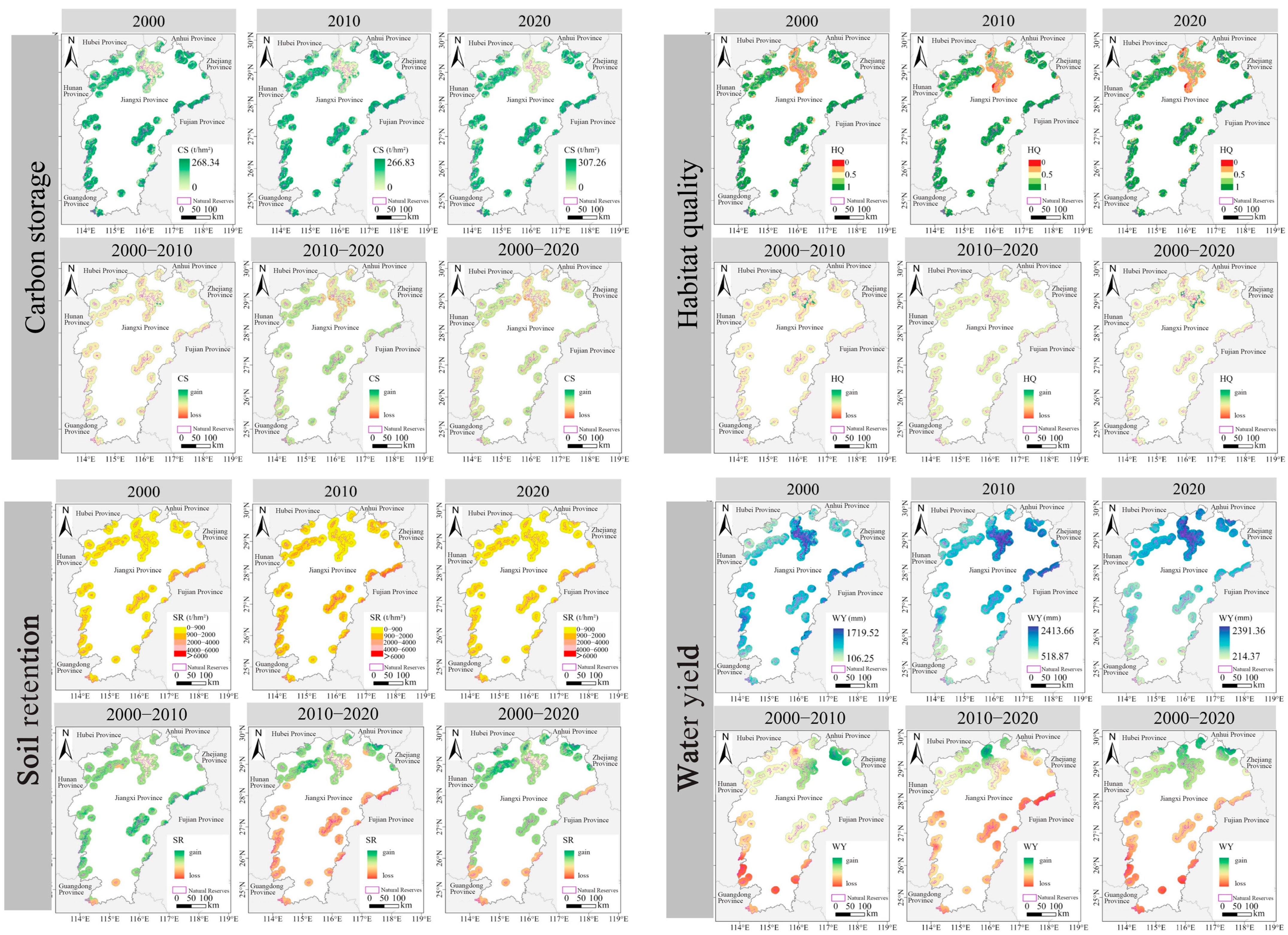
Spatially, from 2000 to 2020, the four key ESs—CS, HQ, SR, and WY—exhibited marked spatial heterogeneity across NRs in Jiangxi Province, China. CS showed pronounced spatial divergence, with relatively low values concentrated in reserves located in the Poyang Lake region of northern Jiangxi, while high values were predominantly found in reserves in the southern part of the province. HQ displayed a similar pattern, with low-value areas mainly concentrated within reserves in the northern Poyang Lake region (Figure 3).

3.1.2. The Assessment of CESI

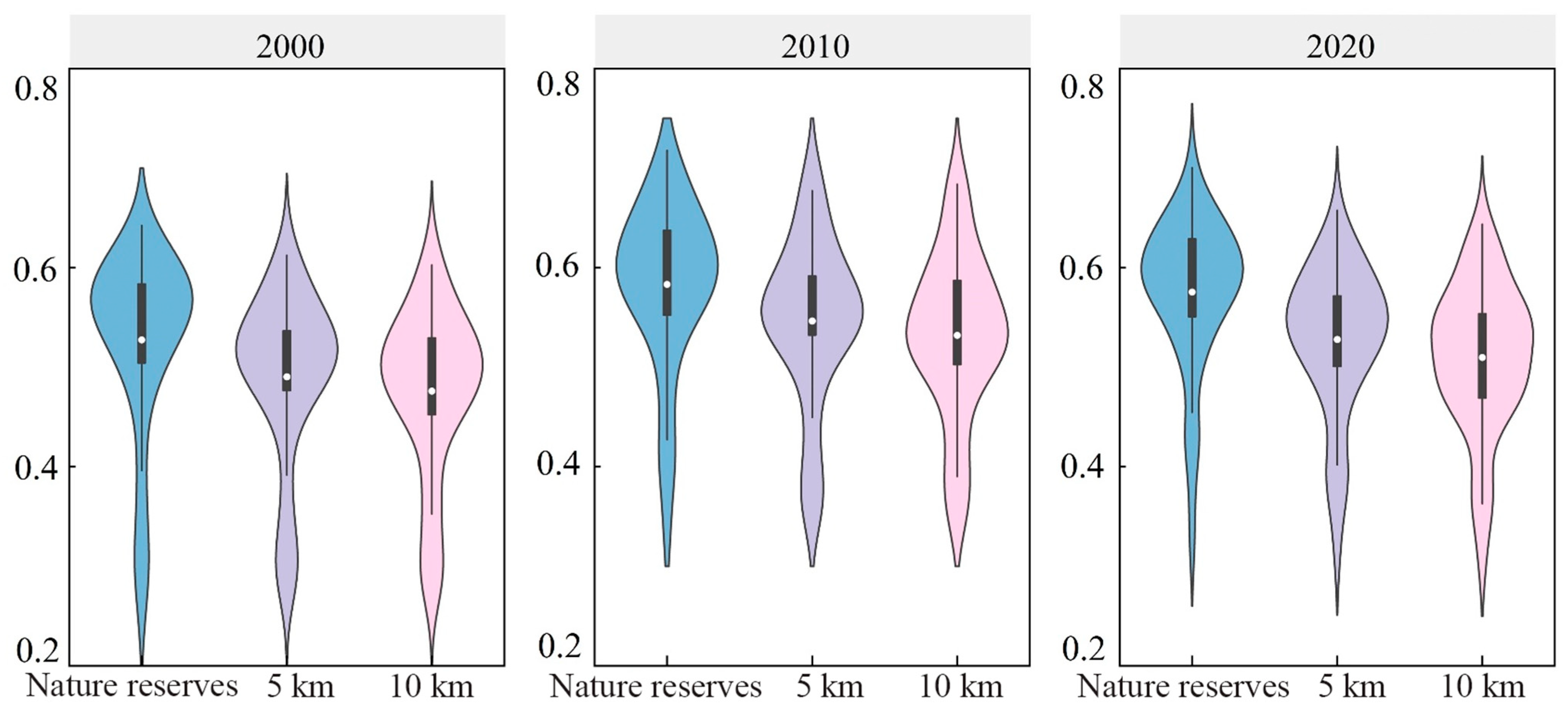
From 2000 to 2020, the overall ecosystem service benefits of NRs in Jiangxi Province remained at a moderate level but followed a pattern of initial increase followed by a slight decline (Figure 4). The CESI rose from 0.486 in 2000 to a peak before decreasing slightly to 0.545 in 2020. Based on the mean area distribution of CESI values over the study period, high-benefit zones accounted for the largest proportion of reserve areas (45.18%), followed by medium-benefit zones (35.01%), while low-benefit zones comprised a smaller share (19.81%).
A comparison of ecosystem service benefits between reserves and their surrounding zones (Figure 4) revealed the following order: NRs (0.53) > 5 km zones (0.50) > 10 km zones (0.49). This indicates that ecosystem service benefits were consistently higher within reserves and exhibited a gradual decline moving outward toward the surrounding zones.
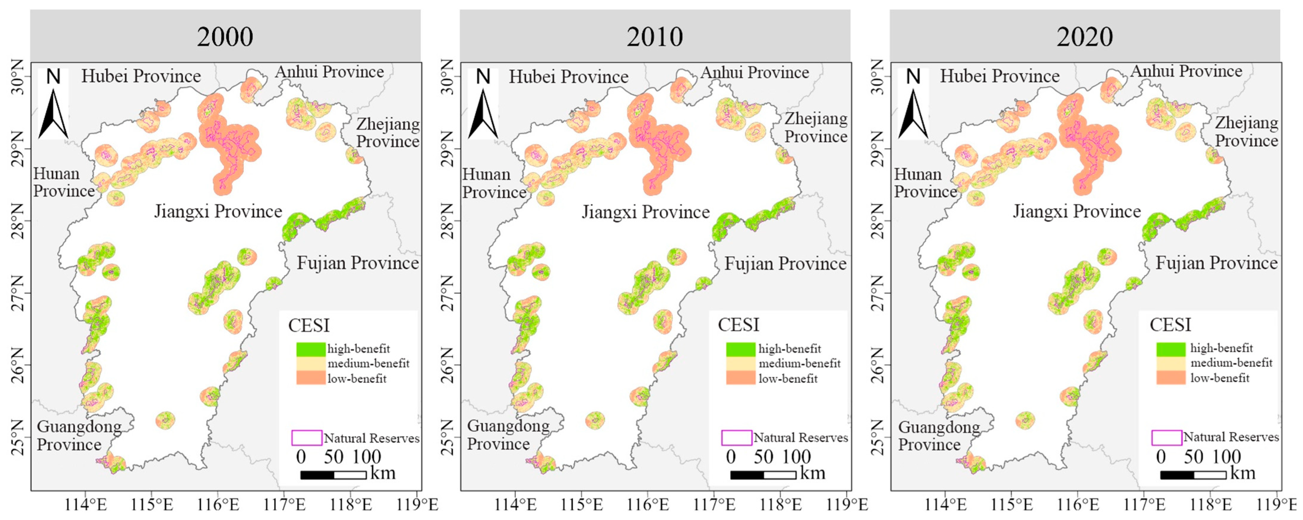
Spatially, Figure 5 shows that reserves in northern Jiangxi had lower CESI values than those in the south. During 2000–2020, five reserves recorded low conservation effectiveness (CESI ≤ 0.4), including the Poyang Lake Migratory Bird Reserve (0.38), Nanji Wetland Reserve (0.34), Duchang Migratory Bird Reserve (0.39), Poyang Lake Carp Reserve (0.39), and Poyang Lake Silverfish Reserve (0.30). In addition, the spatiotemporal variations in the comprehensive ecosystem service indices for each reserve are presented in Figure 5.
These findings highlight that, while NRs in Jiangxi generally maintain moderate to high ecosystem service effectiveness, spatial disparities persist, with northern reserves facing greater conservation challenges than those in the south.

3.2. Dynamic Relationships in the Spatiotemporal Trade-Offs and Synergies of ESs

3.2.1. Spatial Characteristics of Trade-Offs and Synergies

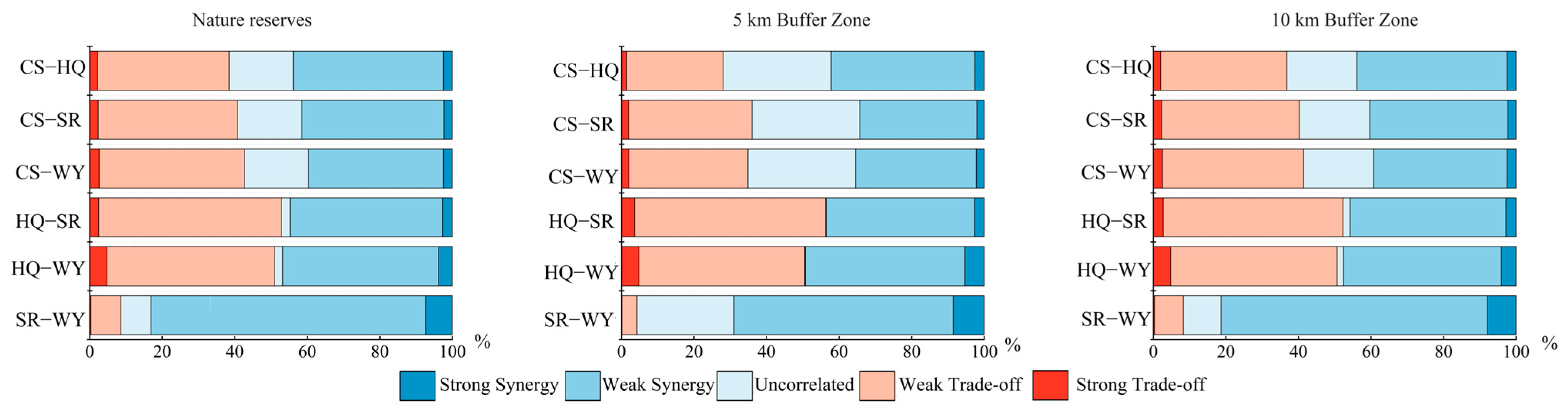
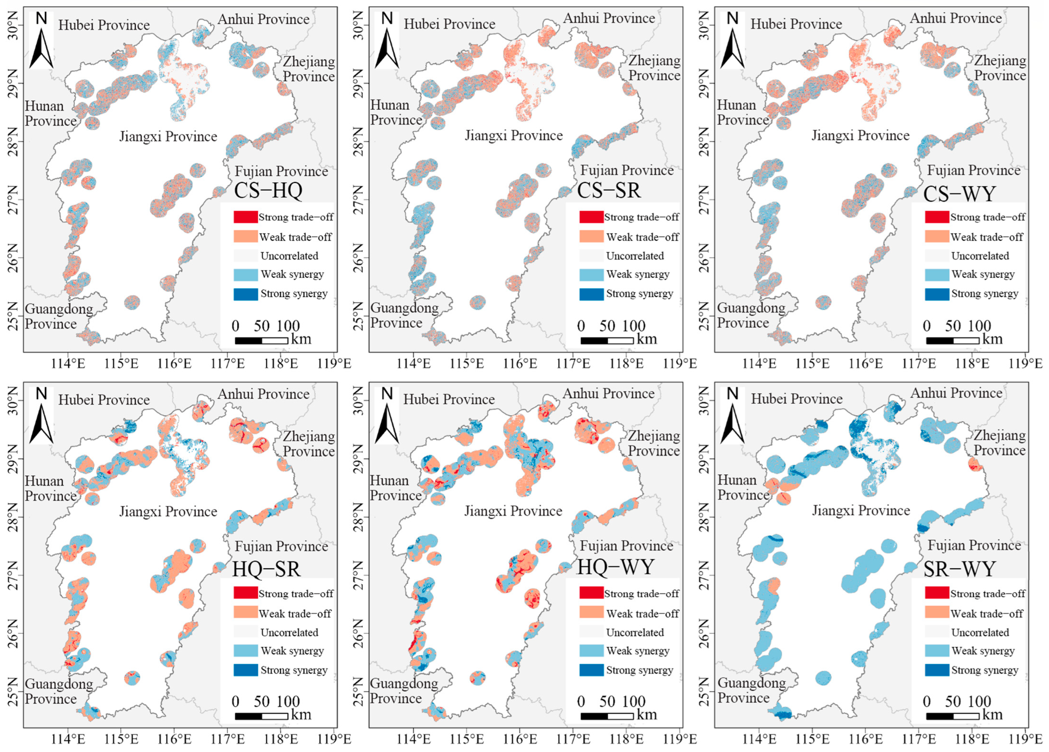
Ecosystem service trade-offs and synergies exhibited pronounced spatial differentiation across NRs. In the Poyang Lake region, between CS and SR (CS–SR), HQ–SR, and HQ–WY were dominated by trade-offs, whereas in southern Jiangxi, CS–SR and SR–WY were primarily characterized by synergies (Figure 6). Weak synergies were observed between HQ–CS, CS–WY, and SR–WY, accounting for 39.61%, 35.44%, and 60.43% of the area, respectively. In contrast, weak trade-offs were evident for CS–SR (34.02%), HQ–SR (52.66%), and HQ–WY (50.53%) (Figure 6).
Ninety-one percent of the NRs exhibit a dominant synergistic relationship between SR and WY; 61% show a dominant synergistic relationship between HQ and CS; 57% demonstrate a dominant synergistic relationship between CS and WY; 52% display a dominant synergistic relationship between CS and SR; 50% have a dominant synergistic relationship between HQ and SR; and 41% exhibit a dominant synergistic relationship between HQ and WY. Additionally, we found that weakly synergistic areas also dominate the relationship between HQ and CS within both the 5 km and 10 km zones.
Overall, these patterns suggest that, while trade-offs are more concentrated in the Poyang Lake region, synergies dominate in southern Jiangxi and across most reserves, particularly for SR–WY interactions (Figure 7).

3.2.2. Variation in Trade-Off Intensity

Among the trade-offs and synergies among the four types of ESs from 2000 to 2020, the relationships between CS–HQ (0.30), CS–WY (0.48), and HQ–WY (0.40) were characterized by low trade-offs, whereas those between HQ and SR (0.81), CS–SR (0.53), and SR–WY (0.51) were characterized by high trade-offs. In terms of temporal trends, four ecosystem service pairs exhibited increasing trade-off intensities: CS–HQ, CS–WY, HQ–SR, and HQ–WY. In contrast, the trade-off intensity between CS–SR declined over time, while SR–WY showed a fluctuating pattern without a clear directional trend (Figure S2).
These findings indicate that, although some ecosystem service interactions have become increasingly competitive over time, others, such as CS–SR, have shifted toward reduced trade-offs, highlighting the dynamic nature of ecosystem service relationships.
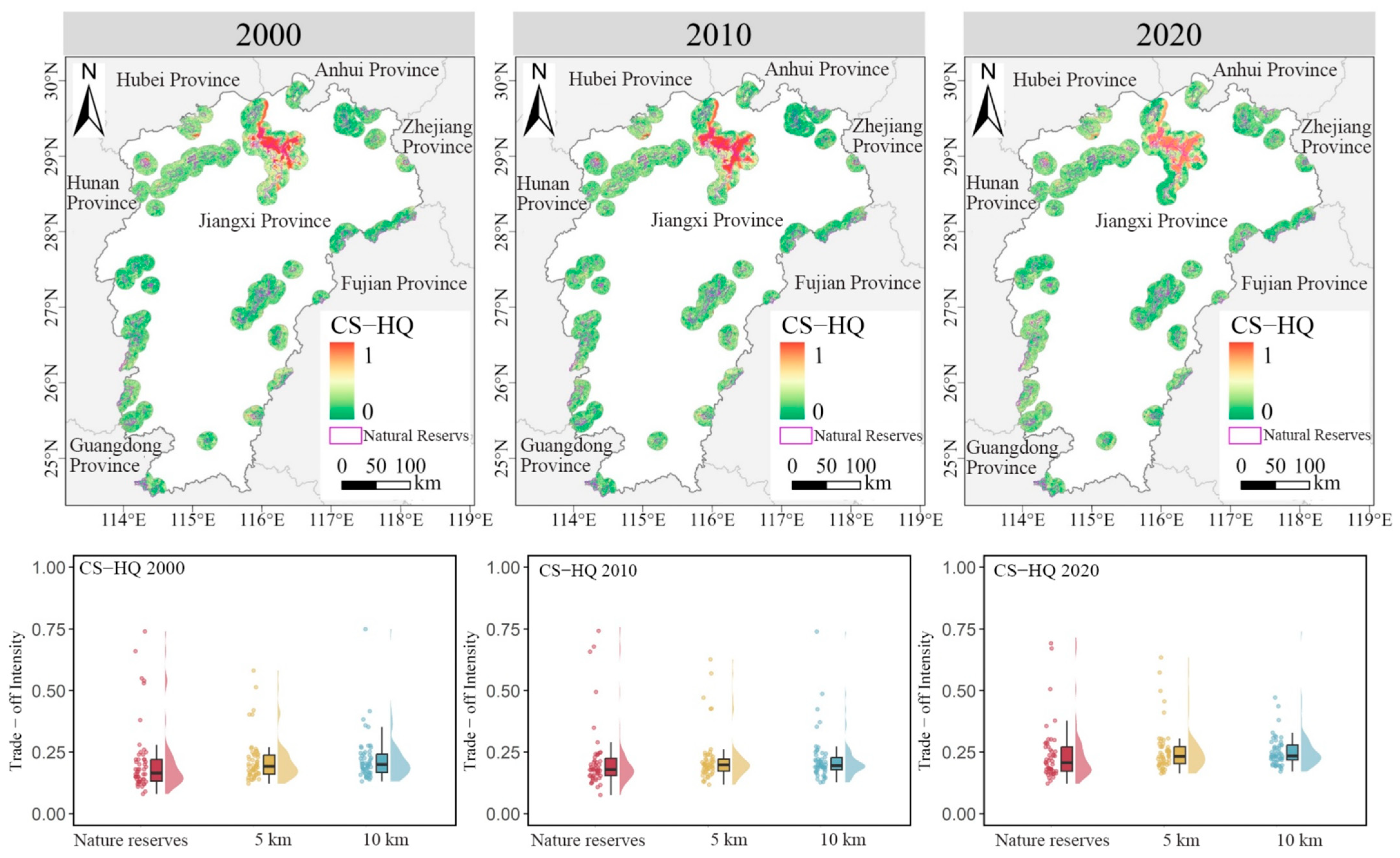
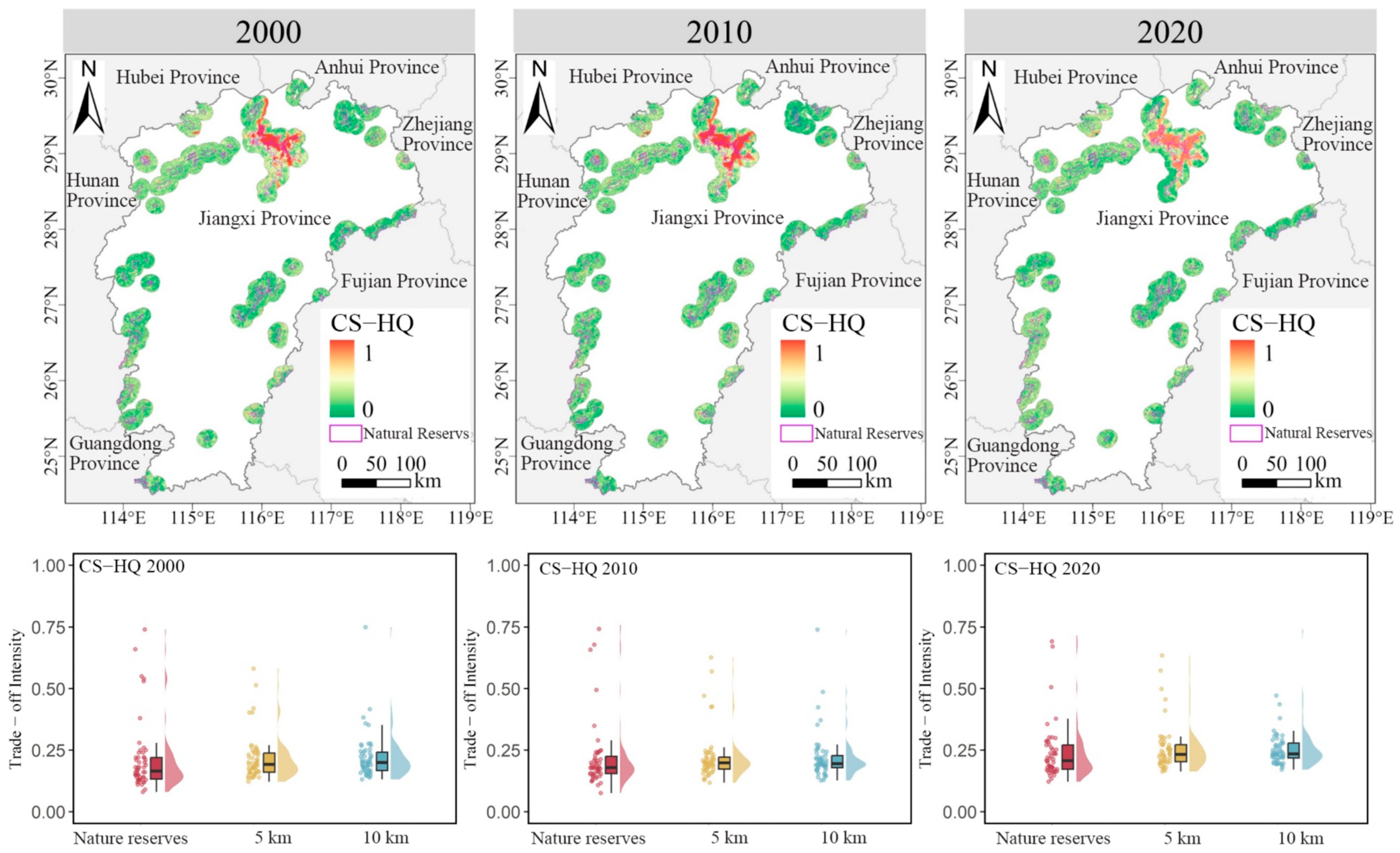
Trade-off intensities among ESs exhibited clear spatial variation. High-intensity trade-offs between CS and HQ were concentrated in reserves within the Poyang Lake region and showed a southward expansion trend during 2000–2020 (Figure 8). The reserves with the highest trade-off intensities included the Poyang Lake Migratory Bird Reserve (0.64), Nanji Wetland Reserve (0.51), Duchang Migratory Bird Reserve (0.66), Poyang Lake Carp Reserve (0.67), and the Yangtze Finless Porpoise Reserve (0.76). These areas were primarily located within the lake zone, where CS was relatively low but HQ remained high, resulting in stronger trade-offs. When compared with surrounding zones (Figure 8), differences in trade-off intensities between reserves and surrounding zones were relatively minor, with both showing an overall increasing trend.
These results suggest that trade-offs between CS and HQ are most pronounced in lake-dominated reserves, and their intensification over time highlights the ecological vulnerability of wetland systems in northern Jiangxi.
The trade-off intensity CS–SR exhibited pronounced spatial heterogeneity. Areas with low trade-off intensity were located within NRs around Poyang Lake and demonstrated a spreading trend from 2000 to 2020 (Figure 9). Eight NRs exhibited low ecosystem service trade-off intensity, predominantly within the lake region. These areas had relatively low CS and SR, resulting in correspondingly low trade-off intensity. Moreover, from 2000 to 2020, trade-off intensity within NRs consistently exceeded that of the 5 km and 10 km surrounding zones (Figure 9).
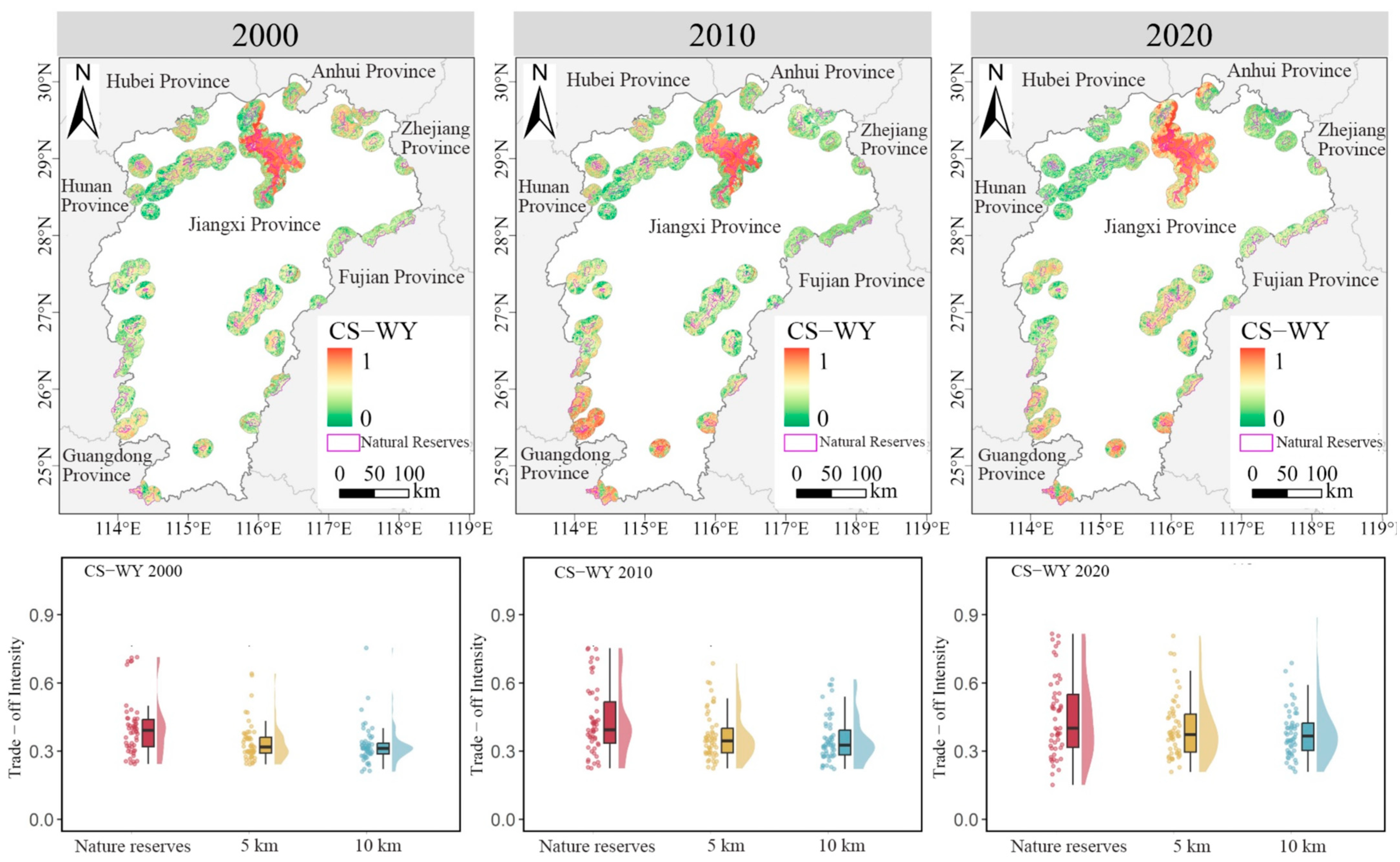
Figure 10 shows that high CS–WY trade-off intensity zones in natural reserves were concentrated in the Poyang Lake region and southern Ganzhou, exhibiting both spatial expansion and a gradual annual increase between 2000 and 2020. From 2000 to 2020, trade-off intensity within natural reserves followed the sequence: NR interiors > 5 km zones > 10 km zones. This pattern primarily reflects high WY but low CS in the Poyang Lake region, leading to elevated trade-off intensity (Figure 10).
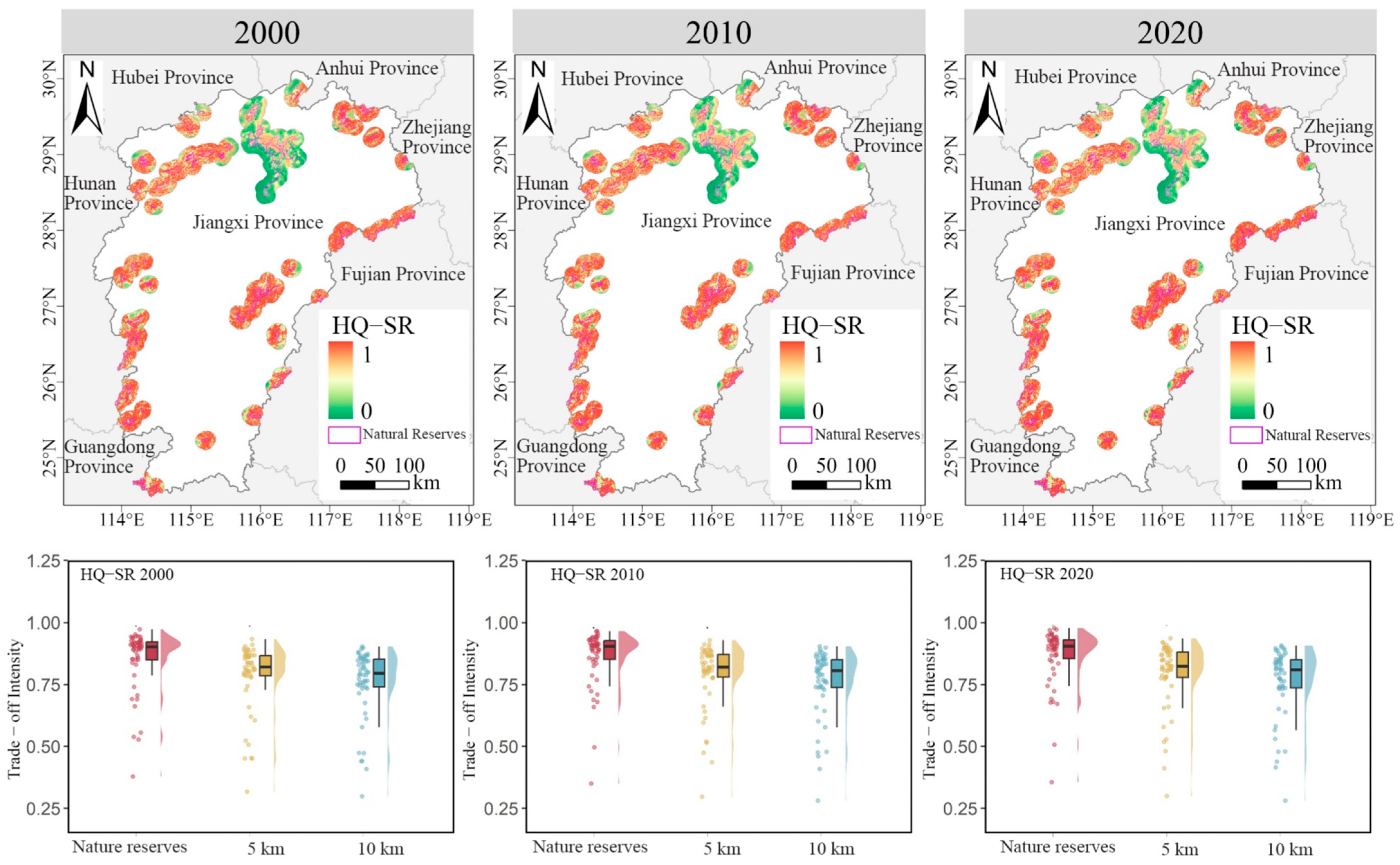
The province-wide HQ–SR trade-off intensity increased steadily over time, reaching a peak of 0.82 in 2020, representing the highest median among the six pairs of ecosystem service trade-offs. Low-intensity areas were mainly distributed around Poyang Lake, where low HQ and SR contributed to reduced trade-off intensity (Figure 11). In contrast, NRs with higher trade-off intensity were characterized by high HQ but relatively low SR, which resulted in elevated trade-off intensity. Furthermore, from 2000 to 2020, HQ–SR trade-off intensity differed markedly between NRs and surrounding zones, following the pattern: nature reserves > 5 km zones > 10 km zones (Figure 11).
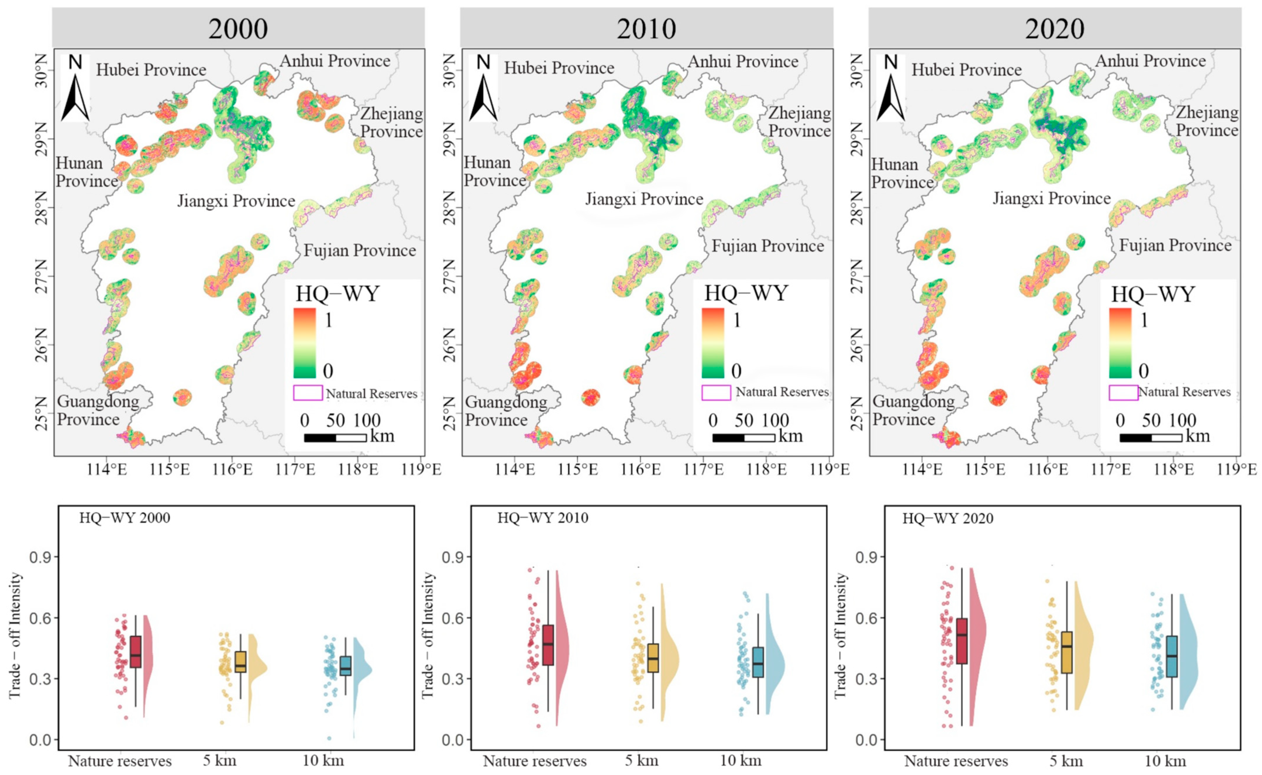
HQ–WY disparity increased across the three observations, with lower values concentrated in northern Jiangxi (Figure 12). Thirty-three NRs showed an increase, and seventeen had a mean value above 0.5; Xinfeng Jinpenshan Nature Reserve had the highest value. Mean disparity was higher inside NRs than in the 5 km and 10 km zones. This relationship describes co-variation between modeled habitat condition and annual water yield.
The trade-off intensity of SR–WY exhibited a fluctuating yet overall declining trend, with minimal differences between natural reserves and surrounding zones; both showed a decreasing pattern (Figure 13). From 2000 to 2020, 57% of NRs experienced a decline in ecosystem service trade-off intensity. Spatially, high trade-off intensity zones were concentrated in the northern and northeastern natural reserves of Jiangxi Province, with the highest intensity observed within the Poyang Lake region (Figure 13). This pattern likely reflects the combination of high WY and low SR in the lake area, resulting in a characteristic high trade-off distribution.

3.3. Multi-Level Potential Driving Factor Analysis

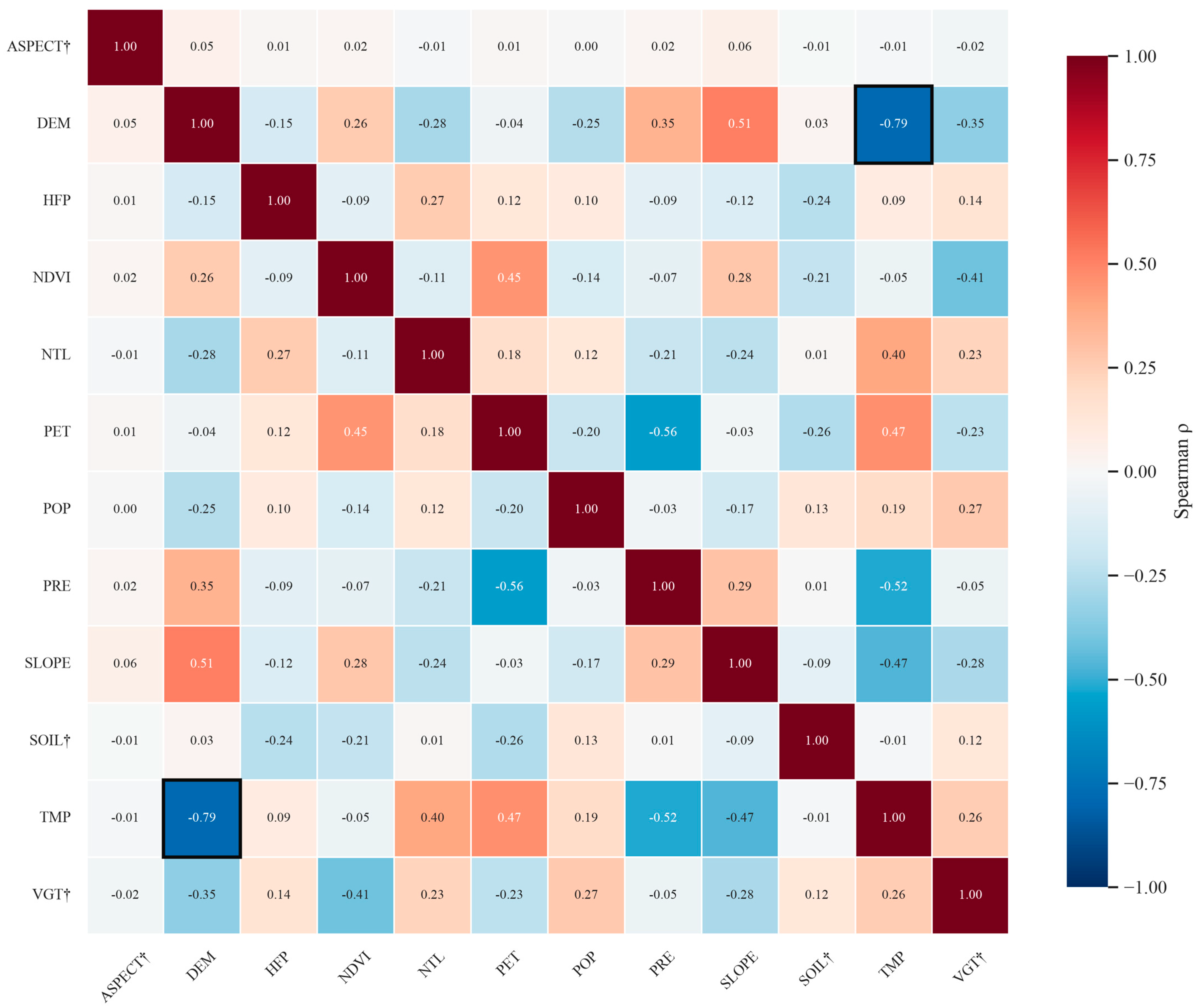
To explore the potential drivers of the four ESs, we used their mean values across the three observation years as response variables and the 2020 environmental variables as the explanatory context. Twelve candidate environmental and anthropogenic variables were initially considered. To reduce circular interpretation, the variables were screened separately for each ES. Variables used directly in the corresponding InVEST module, or closely related to its input data, were excluded from the external-factor analysis. This screening retained nine factors for CS, nine for HQ, five for SR, and three for WY (Table 2). Spearman correlation analysis identified a strong correlation only between DEM and temperature (TMP) (γ = −0.79) (Figure 14). To avoid including both variables in the same service-specific analysis, TMP was retained for CS, whereas DEM was retained for HQ (Figure S3).
Associations based on the three-year mean ES values differed among services. Due to the absence of explicit modeling of spatial dependence among neighboring raster cells, the interpretation focused primarily on coefficient magnitude, and nominal statistical significance was treated cautiously. CS and HQ were mainly related to topography and human pressure. SLOPE showed the strongest positive correlation with both CS (γ = 0.433) and HQ (γ = 0.366), whereas POP and HFP were negatively correlated with these services. Associations with SR were generally weak, with a maximum absolute correlation of 0.265. WY was most strongly correlated with POP (γ = 0.433). Although ASPECT was statistically significant, its effect was negligible for CS (ε2 = 0.004) and small for HQ (ε2 = 0.022). SOIL had larger effects on both CS (ε2 = 0.307) and HQ (ε2 = 0.238) (Table 2).
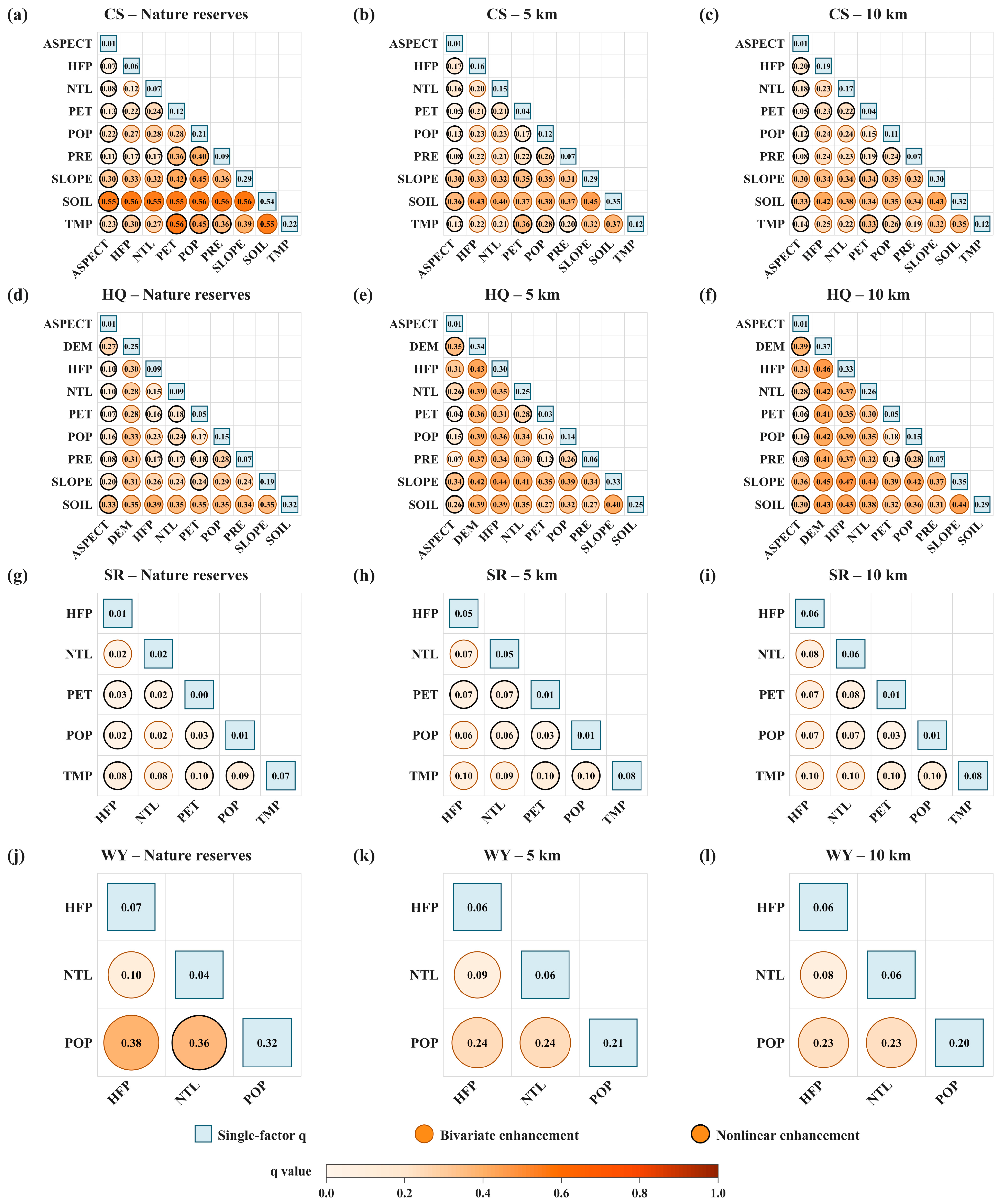
Single-factor GeoDetector results showed no consistent increase in explanatory power from reserve interiors to the surrounding zones (Figure S3). For CS, SOIL had the highest explanatory power, but its q value decreased from 0.539 inside NRs to 0.324 in the 10 km zone. For HQ, the leading factor shifted from SOIL inside NRs to DEM in the surrounding zones. TMP remained the leading factor for SR, although its explanatory power was consistently low (q = 0.075–0.078). POP was the leading factor for WY, but its q value decreased from 0.319 inside NRs to 0.205 in the 10 km zone. These patterns indicate that the factors associated with ES distributions varied by service and spatial context.
All evaluated factor pairs showed either bivariate or nonlinear enhancement in the interaction analysis (Figure 15). For CS, the interaction between SLOPE and SOIL consistently had the highest explanatory power, although its q value decreased from 0.564 within NRs to 0.427 in the 10 km surrounding zone. For HQ, the dominant interaction shifted from HFP and SOIL within NRs to HFP and SLOPE in the surrounding zone. The corresponding maximum q value increased from 0.386 to 0.470. Interactions associated with SR remained weak across all spatial zones (q ≤ 0.105). For WY, the dominant interaction weakened with increasing distance from NRs and shifted from HFP and POP to NTL and POP. Overall, interaction explanatory power was highest for CS and HQ and consistently lowest for SR. These findings indicate that cross-boundary interaction patterns differed among ESs.

4. Discussion

4.1. Cross-Boundary Patterns in the Context of Comparable Protected-Area Studies

The principal empirical pattern was an outward CESI gradient (0.53 within NRs, 0.50 in the 5 km zones, and 0.49 in the 10 km zones), accompanied by service-specific exceptions, such as higher annual WY outside NRs in 2020. The direction is broadly consistent with matched national evidence showing that many Chinese protected areas maintain at least one ES better than comparable unprotected sites [17] and with global evidence that protected areas often resist habitat loss better than matched controls [18]. The magnitude is not directly comparable, however, because those studies used matching or causal designs, whereas our nested zones retain pre-existing differences in terrain, ecosystem type, reserve siting, and land-cover composition. We therefore interpret the gradient as a cross-boundary spatial pattern rather than proof of management effectiveness.
Service trajectories were also heterogeneous. CS and HQ showed small net increases (7.35% and 0.91%), whereas SR and annual WY increased strongly to 2010 and then declined by 15.26% and 13.23%, respectively, by 2020. A recent forest-reserve study in Jiulianshan, Jiangxi, likewise reported that land-cover and climate contributions differed among services [24], while a tropical forest national-park assessment found that HQ could increase even when water-related and soil-related services declined [34]. These comparisons support a service-specific interpretation rather than a single trajectory of ecological improvement. Because our association models use three-year mean responses and mainly 2020 covariates, they cannot identify the causes of the changes from 2000 to 2020.
Lower CESI values were clustered in five Poyang Lake wetland and wildlife reserves. Independent remote-sensing evidence from Poyang Lake shows strong seasonal and interannual hydrological variability, including a long-term decline in dry-season water area while wet-season area remained comparatively stable [35]. Such hydrological variability is a plausible context for the modeled wetland patterns, but it does not demonstrate that drought or river regulation caused the specific CESI values reported here. Differences between provincial-level and national-level reserves likewise should not be attributed to administrative performance without controlling for ecosystem composition, reserve objectives, and baseline conditions.

4.2. Interactive Relationships Between Ecosystem Service Trade-Offs and Synergies

The positive SR–WY association may reflect the combined influence of precipitation, terrain, and vegetation cover. In areas with high precipitation and steep terrain, greater rainfall can increase both modeled water yield and potential erosion. Where vegetation cover reduces actual soil loss, relatively high SR may, therefore, coexist with high WY. This combination provides a plausible explanation for the positive SR–WY relationships observed in parts of southern Jiangxi. Similar synergies between WY and SR have been reported in a semiarid watershed, although their strength varied with climatic and landscape conditions [36,37,38]. Other studies have found that well-vegetated land can provide greater sediment retention but lower water yield because of increased evapotranspiration [39]. The SR–WY relationship is therefore likely to depend on precipitation, topography, vegetation, and land-cover composition. In the present study, it is most appropriately interpreted as a context-dependent spatial association. Further analysis using observations of erosion, streamflow, soil moisture, and seasonal water balance would help determine the hydrological processes underlying this relationship.
The negative HQ–SR and HQ–WY associations may represent differences in the service profiles of forests, wetlands, open water, cropland, and other land-cover types rather than direct conflicts between biodiversity and hydrological or erosion-control functions. Modeled HQ reflects the capacity of land-cover types to provide suitable habitat under different threat levels, but it is not a direct measure of species richness. Similarly, the magnitude of SR depends partly on the underlying erosion risk. A location with low potential erosion may have a relatively low SR value even when its habitat condition is favorable. In densely vegetated areas, higher evapotranspiration may also reduce annual WY while supporting habitat condition and soil protection. Such conditions could contribute to negative HQ–WY relationships without implying ecological degradation. These interpretations remain tentative because the present analysis does not include species observations, vegetation structure, soil-moisture dynamics, or seasonal discharge. Land-cover-specific analyses and field observations would be needed to determine which mechanisms are most relevant in different reserve types. Nevertheless, the observed relationships help identify areas where habitat conservation, erosion control, and hydrological management may require different priorities.
The generally higher CS, HQ, and SR values within NRs are consistent with the expected ecological outcomes of long-term protection. Restrictions on land conversion, reduced human disturbance, vegetation restoration, and forest protection may help maintain carbon stocks, habitat condition, and erosion-control capacity. Previous studies in China have similarly reported that many NRs maintained or enhanced ecosystem services, with stronger outcomes often observed in older reserves or more strictly managed zones [22,23]. A national assessment using statistically matched controls also found that most protected areas enhanced at least one ecosystem service [17]. These findings provide external support for the possibility that protection and management contributed to the higher ES values observed within Jiangxi’s NRs.

4.3. Optimization of Ecosystem Service Functions in NRs

The cross-boundary results support a tiered management strategy. First priority should be given to the five low-CESI reserves around Poyang Lake—Poyang Lake Migratory Bird, Nanji Wetland, Duchang Migratory Bird, Poyang Lake Carp, and Poyang Lake Silverfish reserves—together with their 5 km surrounding zones, where land-use changes can most directly influence wetland edges. Management should track the four component services separately rather than attempting to maximize CESI alone.
In the Poyang Lake region, priority actions should focus on habitat condition, wetland hydroperiod, and shoreline land use. Practical measures include protecting seasonal inundation and mudflat–vegetation mosaics, restoring hydrological connectivity where locally feasible, limiting new reclamation and hard shoreline conversion, and maintaining low-input farmland or ecological set-asides adjacent to sensitive wetland boundaries. Annual WY should not be used as a target for water-storage restoration; hydrological decisions require water level, discharge, hydroperiod, and ecological demand observations.
In southern Jiangxi, where CS, HQ, and SR are generally higher but several service disparities remain strong, management should retain continuous forest cover, avoid road-driven fragmentation, stabilize erosion-prone slopes with native vegetation, and maintain riparian buffers. In surrounding agricultural zones, contour farming, vegetated field margins, and reduced soil disturbance can be targeted to locations with high erosion risk. In urbanizing zones, development controls should prioritize boundary-adjacent habitat corridors, limits on impervious-surface expansion, and ecological connectivity among neighboring reserves. These recommendations are based on the observed spatial patterns and established ecological principles. However, their effectiveness should be carefully validated through site-specific monitoring rather than inferred directly from the associations identified in this study.

4.4. Limitations and Future Directions

When assessing ESs, this study integrated multi-source remote-sensing and environmental datasets. Owing to differences in data sources, spatial resolutions, and observation periods, some uncertainties should be considered when interpreting the results. Although all spatial layers were aligned to a common 30 m grid, several variables were originally available at a 1 km resolution. The resampling procedure improved spatial consistency among datasets but did not increase their original level of spatial detail. The InVEST outputs are model-based estimates and may differ from field observations because they depend on land-cover accuracy, biophysical parameters, threat settings, and the assumptions of individual modules. In particular, HQ represents modeled habitat condition rather than direct biodiversity observations, while annual WY represents modeled water production rather than the full range of water-retention and hydrological-regulation functions. Nevertheless, the recurrence of the main spatial patterns across multiple years and surrounding zones provides confidence in the broad comparative findings, although the exact values and local differences would benefit from field validation. The 2017 reserve boundaries were used as a consistent spatial framework for all observation years because complete historical boundaries were unavailable. Consequently, estimates for the earlier years represent historical landscape conditions within the present-day reserve footprints. The standardized surrounding zones also provided a consistent basis for cross-boundary comparison, although differences among reserve interiors and surrounding landscapes may reflect the combined influence of protection, terrain, ecosystem composition, accessibility, and land-use history. In addition, the three observation years were suitable for identifying decadal changes but provided limited information on interannual variability. The association analyses used three-year mean ES values and covariates representing mainly 2020 conditions, and are therefore more appropriate for identifying spatial associations than temporal responses. Spatial autocorrelation was not explicitly incorporated into the statistical models, and the reserve types were represented unevenly because forest and wildlife reserves constitute most of Jiangxi’s reserve network. These factors may influence model performance and the generalization of results for less-represented reserve types. The equally weighted CESI offered a transparent summary of multiple services, although alternative normalization and weighting schemes may produce some differences in relative rankings. Due to data availability, the analysis did not include detailed information on conservation investment, management intensity, policy implementation, or other reserve-specific socioeconomic conditions that may contribute to ES performance. Future studies could integrate these management variables with time-specific reserve boundaries, longer annual data series, matched comparison areas, multiscale analyses, spatially blocked validation, CESI sensitivity tests, and field observations of biodiversity, soil erosion, and hydrological processes. These improvements would help clarify the mechanisms underlying the observed patterns and provide a more detailed assessment of the contribution of reserve management to ES maintenance.

5. Conclusions

This study compared four modeled ESs across 54 NRs and nested 5 and 10 km surrounding zones in 2000, 2010, and 2020. CS increased by 7.35% and HQ by 0.91% over the two decades. SR increased by 72.06% to 2010 and then decreased by 15.26%, while annual WY increased by 45.92% and then decreased by 13.23%. CESI values followed the pattern: NR interiors (0.53) > 5 km zones (0.50) > 10 km zones (0.49). From 2000 to 2020, carbon storage and habitat quality increased slightly, whereas soil retention and water yield showed an increase followed by a decrease. Carbon storage, habitat quality, and soil retention were generally higher within NRs, and the comprehensive ecosystem service index declined from reserve interiors to the surrounding zones. These patterns suggest that NRs may contribute to maintaining multiple ecosystem services, although differences in environmental conditions and land-use history should also be considered. The relationships among ecosystem services varied across spatial zones. Carbon storage and habitat quality, as well as soil retention and water yield, were predominantly synergistic, whereas the strongest trade-off occurred between habitat quality and soil retention. The factors associated with these services also differed among reserve interiors and surrounding landscapes. Overall, the findings highlight the need to manage NRs together with their surrounding areas and to consider context-dependent trade-offs and synergies when developing conservation strategies.

Supplementary Materials

The following supporting information can be downloaded at: https://www.mdpi.com/article/10.3390/land15091551/s1, Figure S1: Changes in the CESI within the NRs and their buffer zones of Jiangxi Province from 2000 to 2020; Figure S2: Changes in trade-off intensity within the NRs of Jiangxi Province from 2000 to 2020; Figure S3: Importance scores of driving factors for four types of ESs in NRs and surrounding zones of Jiangxi Province. Table S1: National Directory of Nature Reserves in Jiangxi Province (2017).

Author Contributions

Conceptualization, Y.W.; Methodology, Y.W. and F.Z.; Software, Y.W.; Validation, Y.W. and D.G.; Formal analysis, Y.W., D.G., F.Z. and W.Z.; Investigation, Y.W.; Resources, M.D.; Data curation, Y.W., F.Z. and M.D.; Writing—original draft, Y.W., D.G. and F.Z.; Writing—review & editing, Y.W., D.G. and M.D.; Visualization, Y.W., M.D. and W.Z.; Supervision, M.D.; Funding acquisition, M.D. All authors have read and agreed to the published version of the manuscript.

Funding

This research was funded by the Jiangxi Provincial Natural Science Foundation (No. 20252BAC250033), the National Natural Science Foundation of China (NSFC) program (No. 42161021), the Jiangxi Normal University Graduate Student Innovation Fund (No. YJS2024009), and the key research and development projects of China Railway Corporation (No. 2023-major-05).

Data Availability Statement

The data that support the findings of this research are available from the corresponding author, [MJD], upon reasonable request.

Conflicts of Interest

Author Yonggang Wang was employed by the company China Railway Water Conservancy and Hydropower Planning and Design Group Co., Ltd. The remaining authors declare that the research was conducted in the absence of any commercial or financial relationships that could be construed as a potential conflict of interest.

References

  1. Costanza, R.; d’Arge, R.; de Groot, R.; Farber, S.; Grasso, M.; Hannon, B.; Limburg, K.; Naeem, S.; O’Neill, R.V.; Paruelo, J.; et al. The Value of the World’s Ecosystem Services and Natural Capital. Nature 1997, 387, 253–260. [Google Scholar] [CrossRef] [Scilit]
  2. Curtis, P.G.; Slay, C.M.; Harris, N.L.; Tyukavina, A.; Hansen, M.C. Classifying Drivers of Global Forest Loss. Science 2018, 361, 1108–1111. [Google Scholar] [CrossRef] [Scilit]
  3. Convention on Biological Diversity (CBD). Kunming–Montreal Global Biodiversity Framework; Decision 15/4, CBD/COP/DEC/15/4. In Proceedings of the Conference of the Parties to the Convention on Biological Diversity, Montreal, QC, Canada, 7–19 December 2022. [Google Scholar]
  4. Huang, M.; Gong, D.; Deng, Y.; Ge, Y.; Lin, H.; Zhu, D.; Xiao, C.; Jiang, T.; Altan, O. Spatiotemporal Dynamics of Carbon Balance Considering Multi-Dimensional Urbanization Across 366 Cities in China. Earth’s Future 2026, 14, e2025EF007265. [Google Scholar] [CrossRef] [Scilit]
  5. Watson, J.E.M.; Dudley, N.; Segan, D.B.; Hockings, M. The Performance and Potential of Protected Areas. Nature 2014, 515, 67–73. [Google Scholar] [CrossRef] [Scilit] [PubMed]
  6. Wu, H.; Song, F.; Li, H.; Bai, J.; Cui, L.; Su, F.; Kalantari, Z.; Ferreira, C.S. The Role of Nature Reserves in Ecosystem Services and Urban Ecological Sustainable Development. Land 2025, 14, 136. [Google Scholar] [CrossRef] [Scilit]
  7. Zeng, Y.; Koh, L.P.; Wilcove, D.S. Gains in Biodiversity Conservation and Ecosystem Services from the Expansion of the Planet’s Protected Areas. Sci. Adv. 2022, 8, eabl9885. [Google Scholar] [CrossRef] [Scilit]
  8. Zhao, Y.; Wu, Y.; Han, P.; Wen, Z.; Wang, Z.; Liu, Y.; Hu, E.; Shi, H.; Wang, Z. Mechanistic Drivers and Sustainability Implications of Ecosystem Service Interactions in the Yinshan Mountain Region. Land Degrad. Dev. 2026, 37, 5459–5479. [Google Scholar] [CrossRef] [Scilit]
  9. Marcolin, F.; Mammola, S.; Alba, R.; Segurado, P.; Reino, L.; Chamberlain, D. Socio-Economic Status and Non-Native Species Drive Bird Ecosystem Service Provision in Urban Areas. Glob. Change Biol. 2025, 31, e70311. [Google Scholar] [CrossRef] [Scilit]
  10. Yang, L.; Zhou, X.; Gu, X.; Liang, Y. Impact Mechanism of Ecosystem Services on Resident Well-Being under Sustainable Development Goals: A Case Study of the Shanghai Metropolitan Area. Environ. Impact Assess. Rev. 2023, 103, 107262. [Google Scholar] [CrossRef] [Scilit]
  11. Zhou, Q.; Li, X.; Wang, Y.; Xin, Z.; Musa, A.; Wang, L. Mesophytic and Less-Disturbed Mountainous Habitats Are Important for in Situ Conservation of Rare and Endangered Plants. Glob. Ecol. Conserv. 2023, 44, e02488. [Google Scholar] [CrossRef] [Scilit]
  12. Cord, A.F.; Bartkowski, B.; Beckmann, M.; Dittrich, A.; Hermans-Neumann, K.; Kaim, A.; Lienhoop, N.; Locher-Krause, K.; Priess, J.; Schröter-Schlaack, C.; et al. Towards Systematic Analyses of Ecosystem Service Trade-Offs and Synergies: Main Concepts, Methods and the Road Ahead. Ecosyst. Serv. 2017, 28, 264–272. [Google Scholar] [CrossRef] [Scilit]
  13. Gonçalves-Souza, D.; Vilela, B.; Phalan, B.; Dobrovolski, R. The Role of Protected Areas in Maintaining Natural Vegetation in Brazil. Sci. Adv. 2021, 7, eabh2932. [Google Scholar] [CrossRef] [Scilit]
  14. Howe, C.; Suich, H.; Vira, B.; Mace, G.M. Creating Win-Wins from Trade-Offs? Ecosystem Services for Human Well-Being: A Meta-Analysis of Ecosystem Service Trade-Offs and Synergies in the Real World. Glob. Environ. Change 2014, 28, 263–275. [Google Scholar] [CrossRef] [Scilit]
  15. Liu, Y.; Zhao, W.; Zhang, Z.; Hua, T.; Ferreira, C.S.S. The Role of Nature Reserves in Conservation Effectiveness of Ecosystem Services in China. J. Environ. Manag. 2023, 342, 118228. [Google Scholar] [CrossRef] [Scilit]
  16. Zhao, C.; Su, S.; Gong, Z.; Lv, C.; Li, N.; Luo, Q.; Zhou, X.; Li, S. Effectiveness of Protected Areas in the Three-River Source Region of the Tibetan Plateau for Biodiversity and Ecosystem Services. Ecol. Indic. 2023, 154, 110861. [Google Scholar] [CrossRef] [Scilit]
  17. Yu, C.; Zhang, Z.; Jeppesen, E.; Gao, Y.; Liu, Y.; Liu, Y.; Lu, Q.; Wang, C.; Sun, X. Assessment of the Effectiveness of China’s Protected Areas in Enhancing Ecosystem Services. Ecosyst. Serv. 2024, 65, 101588. [Google Scholar] [CrossRef] [Scilit]
  18. Li, G.; Fang, C.; Watson, J.E.M.; Sun, S.; Qi, W.; Wang, Z.; Liu, J. Mixed Effectiveness of Global Protected Areas in Resisting Habitat Loss. Nat. Commun. 2024, 15, 8389. [Google Scholar] [CrossRef] [Scilit]
  19. Brown, C.J.; Adame, M.F.; Buelow, C.A.; Frassl, M.A.; Lee, S.Y.; Mackey, B.; McClure, E.C.; Pearson, R.M.; Rajkaran, A.; Rayner, T.S.; et al. Opportunities for Improving Recognition of Coastal Wetlands in Global Ecosystem Assessment Frameworks. Ecol. Indic. 2021, 126, 107694. [Google Scholar] [CrossRef] [Scilit]
  20. Hardaker, A.; Styles, D.; Williams, P.; Chadwick, D.; Dandy, N. A Framework for Integrating Ecosystem Services as Endpoint Impacts in Life Cycle Assessment. J. Clean. Prod. 2022, 370, 133450. [Google Scholar] [CrossRef] [Scilit]
  21. Xie, G.; Lu, C.; Cheng, S. Progress in Evaluating the Global Ecosystem Services. Resour. Sci. 2001, 23, 5–9. [Google Scholar]
  22. Zhao, J.; Liu, S.; Wang, Z.; Gao, H.; Feng, S.; Wei, B.; Hou, Z.; Xiao, F.; Jing, L.; Liao, X. The Impact of Land Use and Landscape Pattern on Ecosystem Services in the Dongting Lake Region, China. Remote Sens. 2023, 15, 2228. [Google Scholar] [CrossRef] [Scilit]
  23. Liu, Y.; Fu, B.; Wang, S.; Rhodes, J.R.; Li, Y.; Zhao, W.; Li, C.; Zhou, S.; Wang, C. Global Assessment of Nature’s Contributions to People. Sci. Bull. 2023, 68, 424–435. [Google Scholar] [CrossRef] [Scilit]
  24. Feng, J.; Li, S.; Huang, C.; Tang, F.; Li, Y.; He, G.; Zhang, X.; Chen, F. Effects of Climate Change, Land Use/Cover Change, and Interactions on Ecosystem Services in Jiulianshan National Nature Reserve of Jiangxi Province, China. J. For. Res. 2025, 36, 66. [Google Scholar] [CrossRef] [Scilit]
  25. Cao, M.; Li, J.; Wang, W.; Xia, J.; Feng, C.; Fu, G.; Huang, W.; Liu, F. Assessing the Effectiveness of Water Retention Ecosystem Service in Qinling National Nature Reserve Based on InVEST and Propensity Score Matching Model. Biodivers. Sci. 2021, 29, 617–628. [Google Scholar] [CrossRef] [Scilit]
  26. Fang, L.; Wang, L.; Chen, W.; Sun, J.; Cao, Q.; Wang, S.; Wang, L. Identifying the Impacts of Natural and Human Factors on Ecosystem Service in the Yangtze and Yellow River Basins. J. Clean. Prod. 2021, 314, 127995. [Google Scholar] [CrossRef] [Scilit]
  27. Feng, Z.; Jin, X.; Chen, T.; Wu, J. Understanding Trade-Offs and Synergies of Ecosystem Services to Support the Decision-Making in the Beijing–Tianjin–Hebei Region. Land Use Policy 2021, 106, 105446. [Google Scholar] [CrossRef] [Scilit]
  28. Fang, C.; Cai, Z.; Devlin, A.T.; Yan, X.; Chen, H.; Zeng, X.; Xia, Y.; Zhang, Q. Ecosystem Services in Conservation Planning: Assessing Compatible vs. Incompatible Conservation. J. Environ. Manag. 2022, 312, 114906. [Google Scholar] [CrossRef] [Scilit]
  29. Natural Capital Project. InVEST, 3.16.0a1; Natural Capital Project: Stanford, CA, USA, 2025. [Google Scholar]
  30. Chen, F.; Li, H.; Zhang, A. Ecological risk assessment based on terrestrial ecosystem services in China. Acta Geogr. Sin. 2019, 74, 432–445. [Google Scholar]
  31. Wang, K.P.; Feng, Y.; Qiu, C.L.; Wang, X.Y.; Ma, J.; Zhang, Y.L. Spatial and Temporal Evolution and Drivers of Ecosystem Services in Beijing, Tianjin and the Beijing–Tianjin Ring Urban Agglomeration. Acta Ecol. Sin. 2022, 42, 7871–7883. [Google Scholar] [CrossRef] [Scilit]
  32. Fan, Y.; Gan, L.; Hong, C.; Jessup, L.H.; Jin, X.; Pijanowski, B.C.; Sun, Y.; Lv, L. Spatial Identification and Determinants of Trade-Offs among Multiple Land Use Functions in Jiangsu Province, China. Sci. Total Environ. 2021, 772, 145022. [Google Scholar] [CrossRef] [Scilit] [PubMed]
  33. Mu, H.; Li, X.; Wen, Y.; Huang, J.; Du, P.; Su, W.; Miao, S.; Geng, M. A Global Record of Annual Terrestrial Human Footprint Dataset from 2000 to 2018. Sci. Data 2022, 9, 176. [Google Scholar] [CrossRef] [Scilit]
  34. Lin, X.; Fu, H. Optimization of Tropical Rainforest Ecosystem Management: Implications from the Responses of Ecosystem Service Values to Landscape Pattern Changes in Hainan Tropical Rainforest National Park, China, over the Past 40 Years. Front. For. Glob. Change 2023, 6, 1242068. [Google Scholar] [CrossRef] [Scilit]
  35. Zhen, H.; Tang, C.; Zhang, S.; Wang, H.; Wu, C.; Sun, J.; Liu, W. Exploring the Vegetation Changes in Poyang Lake Wetlands: Succession and Key Drivers over Past 30 Years. Remote Sens. 2025, 17, 1370. [Google Scholar] [CrossRef] [Scilit]
  36. Chen, S.; Wang, W.; Xu, W.; Wang, Y.; Wan, H.; Chen, D.; Tang, Z.; Tang, X.; Zhou, G.; Xie, Z.; et al. Plant Diversity Enhances Productivity and Soil Carbon Storage. Proc. Natl. Acad. Sci. USA 2018, 115, 4027–4032. [Google Scholar] [CrossRef] [Scilit]
  37. Chen, S.; Liu, X. Spatio-Temporal Variations of Habitat Quality and Its Driving Factors in the Yangtze River Delta Region of China. Glob. Ecol. Conserv. 2024, 52, e02978. [Google Scholar] [CrossRef] [Scilit]
  38. Huang, T.; Yu, D. Water-Soil Conservation Services Dynamic and Its Implication for Landscape Management in a Fragile Semiarid Landscape. Ecol. Indic. 2021, 130, 108150. [Google Scholar] [CrossRef] [Scilit]
  39. Ureta, J.C.; Clay, L.; Motallebi, M.; Ureta, J. Quantifying the Landscape’s Ecological Benefits—An Analysis of the Effect of Land Cover Change on Ecosystem Services. Land 2020, 10, 21. [Google Scholar] [CrossRef] [Scilit]
Figure 1. Distribution of NRs in Jiangxi Province and their nested 5 km and 10 km surrounding zones.
Land 15 01551 g001
Figure 2. Temporal changes in CS (a), HQ (b), SR (c), and WY (d) within the NRs and their surrounding zones in Jiangxi Province.
Land 15 01551 g002
Figure 3. The spatial distribution of CS, HQ, SR, and WY in the NRs and their surrounding zones of Jiangxi Province from 2000 to 2020.
Land 15 01551 g003
Figure 4. Temporal changes in the CESI within the NRs and their surrounding zones in Jiangxi Province from 2000 to 2020.
Land 15 01551 g004
Figure 5. Spatial patterns of the CESI in the NRs and their surrounding zones of Jiangxi Province from 2000 to 2020.
Land 15 01551 g005
Figure 6. Trade-off relationship between NRs and their surrounding zones in Jiangxi Province.
Land 15 01551 g006
Figure 7. Spatial distribution of trade-offs and synergies between NRs and surrounding zones in Jiangxi Province.
Land 15 01551 g007
Figure 8. Spatial distribution and average changes in CS–HQ trade-off intensity in the NRs and surrounding zones of Jiangxi Province from 2000 to 2020.
Land 15 01551 g008
Figure 9. Spatial distribution and average changes in CS–SR trade-off intensity in the NRs and surrounding zones of Jiangxi Province from 2000 to 2020.
Land 15 01551 g009
Figure 10. Spatial distribution and average changes in CS–WY trade-off intensity in the NRs and surrounding zones of Jiangxi Province from 2000 to 2020.
Land 15 01551 g010
Figure 11. Spatial distribution and average changes in HQ–SR trade-off intensity in the NRs and surrounding zones of Jiangxi Province from 2000 to 2020.
Land 15 01551 g011
Figure 12. Spatial distribution and average changes in HQ–WY trade-off intensity in the NRs and surrounding zones of Jiangxi Province from 2000 to 2020.
Land 15 01551 g012
Figure 13. Spatial distribution and average changes in SR–WY trade-off intensity in the NRs and surrounding zones of Jiangxi Province from 2000 to 2020.
Land 15 01551 g013
Figure 14. Spearman correlation matrix among 12 environmental variables (black outlines indicate |γ| ≥ 0.70). The ⟊ symbol represents a categorical environmental factor.
Land 15 01551 g014
Figure 15. Interaction-detector q values for eligible external drivers of four ESs within NRs (a,d,g,j)and the 5 km (b,e,h,k) and 10 km (c,f,i,l) surrounding zones in Jiangxi Province. Diagonal squares show single-factor q values; circles show enhanced two-factor q values.
Land 15 01551 g015
Table 1. Data sources.
Data NamePurposeResolutionTime PeriodSource
Land useWY, HQ, CS30 m2000, 2010, 2020http://www.resdc.cn/
Soil dataDriving factor for SR and WY1000 m2009http://www.ncdc.ac.cn/
DEMDriving factor for SR and WY30 m2009http://www.gscloud.cn/
Meteorological dataDriving factor for SR and WY30 m2000, 2010, 2020http://data.cma.cn/
NDVIDriving factor1000 m2020http://modis.gsfc.nasa.gov/
Population densityDriving factor1000 m2020http://www.resdc.cn/
Vegetation typeDriving factor2020http://www.resdc.cn/
Nighttime lightsDriving factor1000 m2020http://www.resdc.cn/
Human footprintDriving factor1000 m2020[33]
Nature reservesDemarcation of protected area boundaries2017http://www.zrbhq.com.cn/
Table 2. Correlation analysis between ESs and driving factors in the NRs of Jiangxi Province.
Driving FactorsCSHQSRWY
PET(Evapotranspiration)0.312 ***0.209 ***−0.058 ***--
PRE (Precipitation)0.102 ***0.086 ***----
TMP (Temperature)−0.259 ***--−0.265 ***--
ASPECT0.004 ***0.022 ***----
DEM--0.363 ***----
SLOPE0.433 ***0.366 ***----
HFP (Human footprint)−0.146 ***−0.324 ***−0.079 ***0.112 ***
NTL (Nighttime lights)−0.162 ***−0.256 ***−0.073 ***0.127 ***
POP (Population)−0.326 ***−0.302 ***−0.049 ***0.433 ***
NDVI--------
VGT (Vegetation type)--------
SOIL (Soil type)0.307 ***0.238 ***----
(*** represents p < 0.001; -- indicates that the variable was not analyzed as an independent external factor. The reported p-values were not adjusted for spatial autocorrelation and should therefore be interpreted cautiously.).
Disclaimer/Publisher’s Note: The statements, opinions and data contained in all publications are solely those of the individual author(s) and contributor(s) and not of MDPI and/or the editor(s). MDPI and/or the editor(s) disclaim responsibility for any injury to people or property resulting from any ideas, methods, instructions or products referred to in the content.