Can the Implementation of Smart Agriculture Reduce the Urban–Rural Disparity in Land Use Efficiency? Evidence Based on Digital Agriculture in China

Abstract

The deep integration of digital technologies with agricultural production is reshaping how rural land is used and offers new opportunities for narrowing the urban–rural gap in land use efficiency. Building on theoretical analysis, this study uses panel data for 700 Chinese counties from 2010 to 2024, treats the Digital Agriculture Innovation and Application Base pilot program as a quasi-natural experiment, and applies a double machine learning model to examine the effect of smart agriculture construction on the urban–rural gap in land use efficiency. The results show the following: (1) Smart agriculture construction significantly narrows the urban–rural gap in land use efficiency, with channel evidence pointing to agricultural technological progress, improved capital allocation, and agricultural industrial upgrading. (2) The policy effect is statistically significant only in formerly poverty-stricken counties, counties with higher land-transfer rates, and counties with stronger digital foundations, while Fisher permutation tests do not establish statistically significant cross-group differences. (3) Decomposition results show that the program raises rural land use efficiency and the rural marginal returns to capital and labor while leaving the corresponding urban indicators statistically unchanged, so the observed convergence is driven primarily by rural catch-up rather than urban decline. From a factor allocation perspective, this study clarifies how smart agriculture construction can rebalance urban–rural land resource use while identifying the statistical limits of the heterogeneity and channel evidence.

1. Introduction

China’s agricultural production is still characterized by the coexistence of smallholder-based household farming and expanding scale operations. Small and fragmented plots remain widespread, while land transfer and the development of commercial family farms have gradually promoted larger-scale and more specialized production [1]. This production structure creates practical constraints on the transition toward smart agriculture. Fragmented farmland, relatively high technology costs, gaps in digital infrastructure and technical capacity, and uncertainty about investment returns can restrict the adoption of precision and digital technologies [1,2]. Farmers do not uniformly reject agricultural modernization: evidence from China indicates broad openness to precision-agriculture technologies, but willingness and readiness to adopt them vary substantially with farm scale, perceived economic returns, access to information, financing, and service support [1]. Against this background, public smart agriculture programs can serve not only as technology-demonstration projects but also as institutional interventions that lower adoption barriers and facilitate the transition from traditional, decentralized production toward more digitalized, standardized, and intensive agricultural production.

Land use efficiency has become an important constraint on high-quality county development in China as extensive spatial expansion becomes less sustainable [3,4]. The issue is relational as well as aggregate: urban land benefits from denser concentrations of capital, technology, and industry, whereas rural land is more often constrained by lower technological intensity, fragmented management, and limited factor inputs [5,6,7,8]. The resulting within-county disparity can impede urban–rural factor integration, making improvement on the rural side central to efficiency-enhancing convergence.

Digital technologies, represented by the Internet of Things, big data, artificial intelligence, remote sensing, and intelligent machinery, provide a potential route for improving the precision of agricultural production and the productivity of rural land [9,10]. Since 2017, the Digital Agriculture Innovation and Application Base program has introduced precision production, digital management, and intelligent equipment through successive county-level pilots. This staggered policy setting makes it possible to examine whether a production-oriented digital intervention narrows the urban–rural land use efficiency gap and, crucially, whether convergence occurs through rural catch-up rather than urban contraction.

The adoption constraints observed in China have close international parallels. Evidence from European farms shows that precision-agriculture uptake varies with farm scale, expected returns, investment costs, and regional conditions [11,12]; U.S. evidence likewise documents strong scale gradients in adoption and links precision technologies to technical efficiency [13,14]. Research on smallholders in India and Sub-Saharan Africa highlights information quality, connectivity, affordability, skills, and advisory support as recurring adoption constraints [15,16,17]. These cross-country regularities provide a comparative benchmark for the Chinese case: scale, digital readiness, and complementary services are general boundary conditions, whereas the collective land system and the national pilot designation process are institutionally specific to China.

This study makes three contributions. First, it shifts attention from the level of agricultural productivity to convergence within the county urban–rural land use system and distinguishes rural catch-up from urban contraction. Second, it treats agricultural technological progress, capital allocation improvement, and agricultural industrial upgrading as complementary transmission channels rather than isolated mechanisms, clarifying their theoretical connections and the limits of comparing their relative magnitudes. Third, it uses DML to flexibly partial out high-dimensional and nonlinear observed confounding while treating the conventional TWFE event study as an auxiliary diagnostic in view of the staggered timing of treatment.

2. Literature Review

Existing research on digital agriculture identifies several routes through which technology can affect agricultural and land productivity. One strand emphasizes production efficiency: sensing, data analytics, variable-rate technologies, and other precision-agriculture tools can improve input targeting and technical efficiency [10,13,18,19,20]. A second strand focuses on information and coordination. Digital advice, data platforms, and agricultural knowledge networks can reduce information frictions, support technology adoption, and strengthen coordination across production and value chains [9,15,17,21,22,23,24]. A third strand highlights farm scale and fixed costs. Cross-regional evidence from Europe and the United States, together with reviews of small-scale precision farming, shows that farm size and the ability to spread technology costs materially condition adoption [11,12,14,25,26].

The same literature also identifies constraints that can limit or unevenly distribute digital agriculture gains. High up-front costs, limited skills, weak connectivity, and insufficient complementary services can slow adoption, especially among smaller farms and resource-constrained producers [12,15,16,25]. Data governance, trust, advisory capacity, and the organization of agricultural innovation systems can further shape whether digital tools are converted into effective production decisions [9,24,27,28,29]. These constraints imply that digitalization can widen rather than narrow performance differences when access to capital, infrastructure, skills, and services is highly unequal, a concern documented particularly in smallholder settings [16,30].

Comparative evidence therefore points to conditional rather than universal effects. European studies emphasize the roles of farm structure and adoption costs [11,12,19], U.S. evidence shows that adoption is closely related to farm scale [13,14], and field evidence from India and other developing-country settings shows that digital advisory services depend on trust, information quality, connectivity, and complementary support [17,21,22]. Evidence from Sub-Saharan Africa similarly identifies affordability, infrastructure, skills, and institutional support as central barriers for smallholders [15,16]. These results closely mirror the boundary conditions examined later in this study while also showing that the institutional route through which those constraints operate may differ across countries.

Against this international literature, the unresolved issue is not an absence of research on digital agriculture itself. Rather, three more specific gaps remain. First, most studies evaluate farm productivity, technology adoption, technical efficiency, income, or environmental performance, while the relative efficiency of urban and rural land within the same local land system is rarely the outcome of interest [9,11,13,19,20]. Second, technological progress, factor allocation, and rural industrial integration are often examined separately even though digital transformation can connect these processes through information, investment, and value-chain coordination [9,24,31,32]. Third, conventional linear specifications can be restrictive when policy selection and outcomes depend on high-dimensional and nonlinear county characteristics. Accordingly, this study examines whether the staggered Digital Agriculture Innovation and Application Base program changes the within-county urban–rural gap in land use efficiency, how the adjustment is distributed between the rural and urban sides, and which complementary conditions shape the observed response.

3. Institutional Background and Theoretical Analysis

3.1. Institutional Background

Smart agriculture construction is an important institutional arrangement formed against the background of the Digital China initiative and the in-depth advancement of the rural revitalization strategy. For a long time, Chinese agriculture has been dominated by traditional production methods, characterized by limited precision, low resource efficiency, and short industrial chains; rural land output has long lagged behind urban land, and the urban–rural gap in land use efficiency has been pronounced. To promote the digital transformation of agriculture and accelerate agricultural modernization, the relevant national authorities launched the construction of Digital Agriculture Innovation and Application Bases (pilots) in 2017. Relying on the Internet of Things, big data, artificial intelligence, and intelligent equipment, the bases carry out digital transformation in grain, cash crops, livestock and poultry, and aquaculture; explore models and pathways for smart agriculture; and are designated and announced in successive batches. In terms of policy content, smart agriculture construction is not only an agricultural technology-upgrading project but also carries a functional orientation toward optimizing agricultural factor allocation and promoting agricultural industrial upgrading. On the one hand, by introducing digital technologies and intelligent equipment, the program raises the precision and intensification of agricultural production and improves the allocation of land, water, fertilizer, and labor, providing technological support for higher rural land output. On the other hand, by developing digitalized, standardized, and scaled production, the program promotes the integration of agriculture with processing, logistics, and services and extends agricultural value chains, creating conditions for rural land to shift from inefficient to efficient use.

China’s land institutions are also central to interpreting the empirical design. Land in urban areas is state-owned, whereas rural and suburban land is generally collectively owned; farm households hold contractual and land management rights, and agricultural operation can be reorganized through lawful transfer or leasing of land management rights without transferring collective ownership [33,34]. National land survey and cadastral rules distinguish agricultural land from construction land and provide the classification framework from which the study’s rural agricultural land and urban construction land measures are assembled [35]. The county land-transfer rate is therefore a meaningful indicator of whether fragmented management rights have been consolidated into operating units that are better able to absorb machinery and precision technologies. “Formerly poverty-stricken counties” refers to counties previously included in China’s national poverty-targeting classification [36].

3.2. Theoretical Analysis

The urban–rural gap in land use efficiency is defined here as a within-county relative disparity in output density between two land use subsystems: urban construction land supporting secondary- and tertiary-industry output, and rural agricultural land supporting primary-industry output. Because the two subsystems produce different outputs on different land categories, the gap is a scale-free relative measure of output density rather than a like-for-like comparison of production technologies; what it captures is how unevenly economic output is generated per unit of land across the urban and rural subsystems of the same county. The formation and the narrowing of the gap can also operate through fundamentally different mechanisms on the two sides: urban land use efficiency is shaped primarily by agglomeration economies, industrial composition, and the management of construction land supply [3,5,6,7,8], whereas rural land use efficiency depends on agricultural technology, factor allocation, and the scale of operation [11,13,26,37]. The index itself is symmetric: a smaller gap could arise from higher rural efficiency, lower urban efficiency, or simultaneous changes on both sides, and these possibilities have different economic meanings. Because the Digital Agriculture Innovation and Application Base program directly targets agricultural production, its principal adjustment margin is expected to lie on the rural side: urban land already benefits from denser concentrations of capital, technology, and industry, whereas smart agriculture applications can release rural output previously constrained by information, technology, and factor allocation frictions. The theoretically relevant form of convergence is therefore rural catch-up rather than urban decline; Section 6.2.1 later separates the two sides empirically so that the side of adjustment is identified rather than assumed.

Hypothesis H1.

Smart agriculture construction narrows the urban–rural gap in land use efficiency primarily through rural catch-up, that is, by increasing rural land use efficiency without requiring a decline in urban land use efficiency.

From the perspective of technological progress, the primary driver of rural catch-up in land use efficiency is the upgrading of agricultural technology. Agricultural production in rural areas has long relied on experience and traditional methods, with low technological content and extensive resource use, leaving the output potential of land unrealized. By introducing the Internet of Things, remote-sensing monitoring, big data analytics, and intelligent equipment into agricultural production, smart agriculture construction promotes crop-condition sensing, precision irrigation and fertilization, intelligent pest and disease control, and intelligent machinery operations, shifting agricultural production from extensive to precision modes. Precision production reduces the waste of water, fertilizer, and pesticides and raises resource efficiency on the one hand, while it increases yields and product quality, raising agricultural output per unit of land, on the other hand [20]. Evidence from precision-agriculture research links these tools to measurable gains in input targeting and technical efficiency [10,13,18,19], and digital advisory services can substantially improve the quality and reach of production information [22]. Meanwhile, demonstration projects and agricultural advisory networks can lower the threshold for surrounding farmers to learn and use modern technologies [23]. Cross-country studies nevertheless show that such gains depend on complementary skills, connectivity, and service support, so a public demonstration program that bundles equipment, data platforms, and technical guidance would address precisely the constraints that slow private adoption [15,16,30]. Where land management rights can be consolidated through lawful transfer, these technologies are also more readily combined with appropriately scaled operation [37,38]. As agricultural technology improves, rural output per unit of land catches up with urban levels more quickly, narrowing the urban–rural gap in land use efficiency. Accordingly, Hypothesis H2 is proposed.

Hypothesis H2.

Smart agriculture construction narrows the urban–rural gap in land use efficiency by promoting agricultural technological progress.

From the perspective of capital allocation, the second driver of rural catch-up is the relaxation of capital constraints. Rural areas have long suffered from underinvestment in farmland infrastructure, production equipment, digital facilities, and technology application, which limits the productive potential of land. By establishing demonstrations of digitalized production and raising the expected returns on agricultural investment, smart agriculture construction attracts industrial, social, and financial capital into agriculture, providing new sources of investment in digital infrastructure, intelligent equipment, and technological upgrading for rural land [7,8,32]. Digitalization also makes agricultural production more observable and verifiable, which lowers information asymmetries in rural financing and helps convert investment demand into realized capital formation [17,21,39]. The new capital improves irrigation, storage, cold-chain, and intelligent equipment conditions and strengthens the capacity of rural land to support scaled, standardized, and intensive production. At the same time, smart agriculture shifts capital from inefficient, dispersed traditional segments toward digitalized, intensive, high-efficiency segments, alleviating capital misallocation between urban and rural areas [5,6,7,8]. In the misallocation literature, output losses arise when the allocation of capital across uses departs from the allocation implied by relative productivities; policies that redirect capital toward its higher-return rural uses therefore raise aggregate land output for given factor totals [5,6,7]. Because rural capital is relatively scarce, the marginal improvement generated by additional capital exceeds that in capital-abundant urban areas. As capital misallocation declines, the matching between rural land and capital improves, rural output per unit of land accelerates its catch-up, and the urban–rural gap narrows. Accordingly, Hypothesis H3 is proposed.

Hypothesis H3.

Smart agriculture construction narrows the urban–rural gap in land use efficiency by correcting capital misallocation.

From the perspective of industrial structure, the third driver of rural catch-up is agricultural industrial upgrading. Traditional agriculture remains confined to cultivation, breeding, and primary production; weak connections among processing, storage, logistics, and marketing limit agricultural value added and the returns to land operation [9,31]. Digital platforms, e-commerce, and knowledge networks lower the coordination costs that have historically kept processing, logistics, and marketing weakly connected to primary production [24,32]. Through digital transformation and standardized production, smart agriculture construction promotes the integration of agriculture with processing, distribution, and services; extends agricultural value chains; upgrades products from primary goods toward deep processing and branded products; and fosters the integrated development of the primary, secondary, and tertiary industries [9,10,31]. Rural industrial integration supported by digital technologies has been shown to raise the value captured locally from agricultural output and to strengthen the linkage between farm production and downstream demand [31,32]. The extension of value chains and industrial integration raise agricultural value added and land operating returns on the one hand and expand the economic output of agricultural land on the other hand. Because the rural industrial-chain base is relatively weak, the marginal improvement from industrial upgrading is more pronounced, rural land use efficiency accelerates its catch-up, and the urban–rural gap narrows further. Accordingly, Hypothesis H4 is proposed.

Hypothesis H4.

Smart agriculture construction narrows the urban–rural gap in land use efficiency by promoting agricultural industrial upgrading.

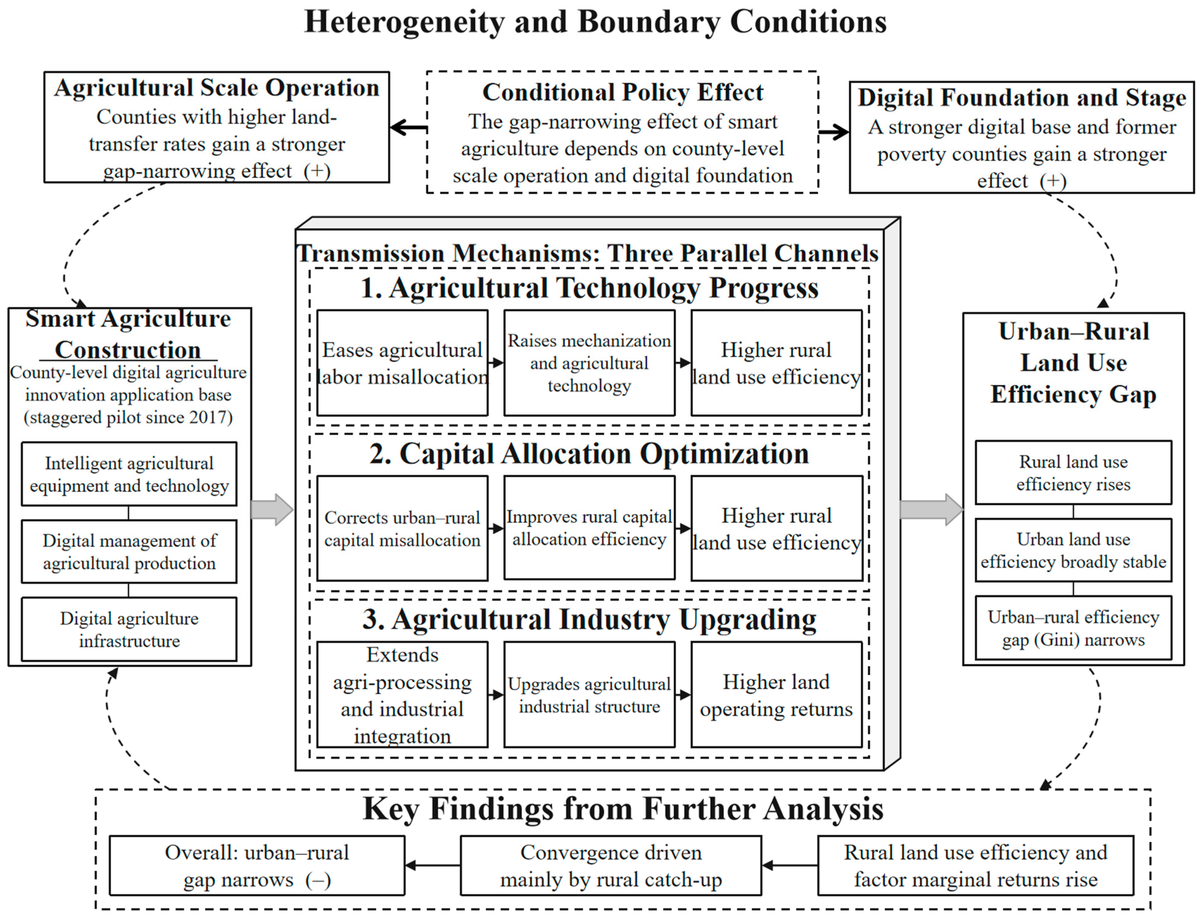
The three channels are complementary rather than mutually exclusive. Agricultural technological progress is the proximate production-efficiency channel: better sensing, information, and precision operations raise the productivity of inputs already used on rural land. Improved information and more observable production processes can reduce financing and allocation frictions, while additional capital supports the adoption of digital equipment and infrastructure. Agricultural industrial upgrading then increases the value captured from agricultural output through processing, logistics, marketing, and agricultural services, which can in turn raise the returns to further technological and capital investment. Accordingly, the channels form a mutually reinforcing configuration rather than three strictly parallel paths (Figure 1). Because ATP, Kmis, and Isu are measured in different units and the channel regressions do not constitute a formal mediation decomposition, their coefficients cannot be compared directly to rank quantitative importance.

3.3. Boundary Conditions and Ex Ante Heterogeneity Hypotheses

The policy effect may depend on the conditions under which digital technologies are absorbed; three ex ante boundary conditions, understood as conditions rather than deterministic treatment–effect rankings, are developed here and evaluated later with both subgroup estimates and formal between-group Fisher permutation tests. The first boundary condition is agricultural scale operation. Intelligent machinery, precision management, and data-intensive field operations involve substantial fixed costs and coordination requirements, so their per-unit cost falls rapidly with contiguous and scaled operation [11,25,26]. Counties with higher land-transfer rates have converted more fragmented household plots into operating units that can spread these fixed costs and standardize production, and farm-level evidence shows that the adoption of advanced production technologies rises with operational scale [1,37]. Accordingly, Hypothesis H5a is proposed.

Hypothesis H5a.

The gap-narrowing effect of smart agriculture construction is expected to be larger in counties with a higher degree of agricultural scale operation.

The second boundary condition is the digital foundation. Smart agriculture applications are data-intensive: they require network connectivity, digital logistics, platform access, and the local capability to use data-based services [15,16,29]. Counties with a stronger digital economy, proxied here by the density of e-commerce (Taobao) villages, already possess the complementary infrastructure, logistics networks, and digitally experienced producers that lower the cost of absorbing new applications, whereas weak connectivity and skills can leave digital investment underused [30,32]. Accordingly, Hypothesis H5b is proposed.

Hypothesis H5b.

The gap-narrowing effect of smart agriculture construction is expected to be larger in counties with stronger digital foundations.

The third boundary condition is initial development status. Formerly poverty-stricken counties are identified by the national poverty-targeting classification [36] and generally start from weaker agricultural foundations, lower capital intensity, and larger unrealized land-output potential. Development evidence indicates that digital technologies can generate comparatively large gains where baseline information, technology, and market access are weakest, provided complementary support is supplied [16,17,21]; a national program that bundles equipment, infrastructure, and technical services provides exactly such support, so the catch-up margin is expected to be larger in these counties. Accordingly, Hypothesis H5c is proposed.

Hypothesis H5c.

The gap-narrowing effect of smart agriculture construction is expected to be larger in formerly poverty-stricken counties because their weaker initial conditions leave greater scope for rural catch-up.

4. Research Design

4.1. Model Specification

The theoretical analysis implies that both pilot selection and the urban–rural land use efficiency gap may depend on nonlinear combinations of economic development, fiscal capacity, population density, investment, urbanization, and their interactions. A conventional TWFE model imposes additive fixed effects and a prespecified linear functional form for observed covariates; this is useful as a benchmark but can be sensitive to functional form misspecification when the covariate space is high-dimensional. A fully nonparametric specification, by contrast, faces a severe dimensionality problem. The partially linear DML framework developed by Chernozhukov et al. [40] is therefore used for the baseline: flexible learners estimate the high-dimensional nuisance functions, while Neyman-orthogonal scores and cross-fitting reduce sensitivity to first-stage regularization and overfitting. The baseline partially linear model is specified as Equation (1):

$${\mathrm{Gap}}_{it}={\theta }_0{\mathrm{Treat}}_{it}+g\left(X_{it}\right)+U_{it}$$

(1)

where Gap denotes the county-level urban–rural gap in land use efficiency, measured by a two-group Gini coefficient constructed from urban and rural land use efficiency; Treat is the policy indicator, equal to 1 in the year a county is designated as a Digital Agriculture Innovation and Application Base and thereafter and 0 otherwise; $X$ is a high-dimensional set of covariates that includes the controls, their squared terms and pairwise interactions, and county and year fixed-effect dummies; $g\left(·\right)$ is an unknown function linking the covariates to the outcome; and $U$ is an error term satisfying E(U|Treat, X) = 0. The parameter ${\theta }_0$ captures the policy effect of interest. To obtain an unbiased estimate of ${\theta }_0$, an auxiliary regression for the conditional expectation of the treatment is constructed, as shown in Equation (2):

$${\mathrm{Treat}}_{it}=m\left(X_{it}\right)+V_{it}$$

(2)

where $m\left(·\right)$ is the conditional expectation of the treatment given the high-dimensional covariates and V is an error term satisfying E(V|X) = 0. Estimation proceeds by using machine learning algorithms to predict the conditional expectations of the outcome and the treatment and then regressing the resulting residuals on one another. Under Neyman orthogonality, this procedure yields a consistent estimate of ${\theta }_0$. To limit overfitting, the sample is randomly divided at a 1:4 ratio for cross-fitting—models are trained on the training subsample, and residuals are generated on the held-out subsample, with the roles rotated across folds—and the number of cross-validation folds is set to five. Random forests are used as the main learner for the unknown functions. Relative to other generic nonparametric or semiparametric approaches, the practical advantage of DML in this application is that it permits flexible machine learning nuisance estimation while retaining an orthogonal low-dimensional target parameter for the policy indicator.

The program is adopted in successive cohorts after 2017. Under staggered adoption and heterogeneous treatment effects, conventional TWFE event-study coefficients can combine comparisons with different cohort weights and may be contaminated across relative-time periods [41,42]. The baseline DML specification does not use the TWFE treatment coefficient as its primary estimate; nevertheless, it targets a pooled partially linear policy parameter rather than cohort-specific group-time average treatment effects. Accordingly, the TWFE event study in Section 5.2 is interpreted only as an auxiliary diagnostic of pre-policy dynamics, not as a cohort-robust estimator of dynamic treatment effects. This boundary of the design is explicitly acknowledged in Section 7.3.

To clarify whether the program affects the urban–rural gap in land use efficiency through agricultural technological progress, capital misallocation, and agricultural industrial upgrading, the mechanism equation shown in Equation (3) is estimated within the same DML framework:

$$M_{it}={\theta }_m{\mathrm{Treat}}_{it}+g_m\left(X_{it}\right)+e_{it}$$

(3)

where $M$ denotes the mechanism variables: agricultural technological progress (ATP), capital misallocation (Kmis), and agricultural industrial upgrading (Isu); $g_m$(·) is the corresponding unknown function; and e is the error term. The estimation procedure is identical to that of the baseline model. The significance of ${\theta }_m$ indicates whether the program changes each mechanism variable and thereby provides evidence on the channels through which it affects the urban–rural gap in land use efficiency.

Because ATP, Kmis, Isu, and Aser are post-treatment variables, entering them as controls in the baseline outcome equation could condition on policy-induced outcomes and create a bad-controls problem; the baseline DML equation therefore never includes them. Mechanism testing instead follows the three-step procedure detailed in Section 5.6: the first step is the baseline policy effect on the gap; the second step estimates Equation (3), the effect of the policy on each mechanism variable; and the third step augments the outcome equation with one mechanism variable at a time. The third step conditions on a post-treatment variable, so its mediation reading requires sequential ignorability, that is, no unobserved mechanism–outcome confounding conditional on the policy, the controls, and the fixed effects; the results are accordingly interpreted as suggestive channel evidence rather than formal indirect effects, mediation shares, or a causal ordering among channels.

4.2. Variable Definitions

The dependent variable is the urban–rural gap in land use efficiency, measured by a Gini coefficient constructed from urban and rural land use efficiency. Urban land use efficiency is the sum of secondary- and tertiary-industry output divided by urban construction land [43], and rural land use efficiency is primary-industry output divided by agricultural land, which includes cultivated land, orchards, forestland, grassland, land for agricultural water facilities, aquaculture areas, and facility-agriculture land. On this basis, urban and rural land use efficiency are treated as two equally weighted observations within each county, and the urban–rural gap is computed with the standard Gini formula [44,45]. Because the two components are output-to-land ratios rather than a globally harmonized land-use-efficiency indicator, the measurement follows the same logic as international land-use-efficiency assessments that derive built-up and land consumption baselines from consistent settlement-layer data, such as the Global Human Settlement Layer framework developed for the SDG 11.3.1 land-use-efficiency indicator [46,47].

Specifically, the urban and rural land use efficiency values for county i in year t are calculated as shown in Equation (4):

$${\mathrm{ULE}}_{it}^U={\displaystyle \frac{{\mathrm{VA}}_{it}^2+{\mathrm{VA}}_{it}^3}{{\mathrm{UrbanLand}}_{it}}}, {\mathrm{ULE}}_{it}^R={\displaystyle \frac{{\mathrm{VA}}_{it}^1}{{\mathrm{RuralLand}}_{it}}}$$

(4)

where VA¹, VA², and VA³ denote the output values of the primary, secondary, and tertiary industries, respectively; UrbanLand denotes urban construction land; and RuralLand denotes agricultural land.

Second, the urban and rural land use efficiency values are treated as two observations within the same county. The general Gini coefficient is given by Equation (5):

$${\mathrm{Gini}}_{it}={\displaystyle \frac{{\displaystyle {\sum }_{g=1}^n}{\displaystyle {\sum }_{h=1}^n}\left|{\mathrm{ULE}}_{git}-{\mathrm{ULE}}_{hit}\right|}{2n^2{\overline{\mathrm{ULE}}}_{it}}}$$

(5)

where $n$ denotes the number of groups. Because the analysis contains only urban and rural areas ($n$ = 2), mean land use efficiency is given by Equation (6):

$${\overline{\mathrm{ULE}}}_{it}={\displaystyle \frac{{\mathrm{ULE}}_{it}^U+{\mathrm{ULE}}_{it}^R}{2}}$$

(6)

Substituting $n$ = 2 and the mean into Equation (5), the index simplifies to Equation (7):

$${\mathrm{Gap}}_{it}={\displaystyle \frac{\left|{\mathrm{ULE}}_{it}^U-{\mathrm{ULE}}_{it}^R\right|}{2\left({\mathrm{ULE}}_{it}^U+{\mathrm{ULE}}_{it}^R\right)}}$$

(7)

This index is the dependent variable used in the analysis. With two positive and equally weighted components, the two-group Gini is a monotone transformation of the absolute urban–rural efficiency ratio: Gap_it = 0.5 × tanh(|ln(ULE_it^U/ULE_it^R)|/2). A value of 0 represents parity between urban and rural land use efficiency, whereas the upper bound of 0.5 is approached when one sector’s efficiency tends toward zero relative to the other. Thus, the index and the absolute log-ratio rank the degree of disparity in the same order, although a signed log-ratio would additionally encode which side is more efficient.

Conceptually, Gap is a symmetric relative-inequality index rather than a direct decomposition of the causes of urban and rural efficiency. A reduction in Gap alone does not reveal whether convergence comes from rural improvement or urban deterioration. This distinction is central to the interpretation of H1; the two components are therefore estimated separately in Section 6.2.1 to identify the side on which adjustment occurs.

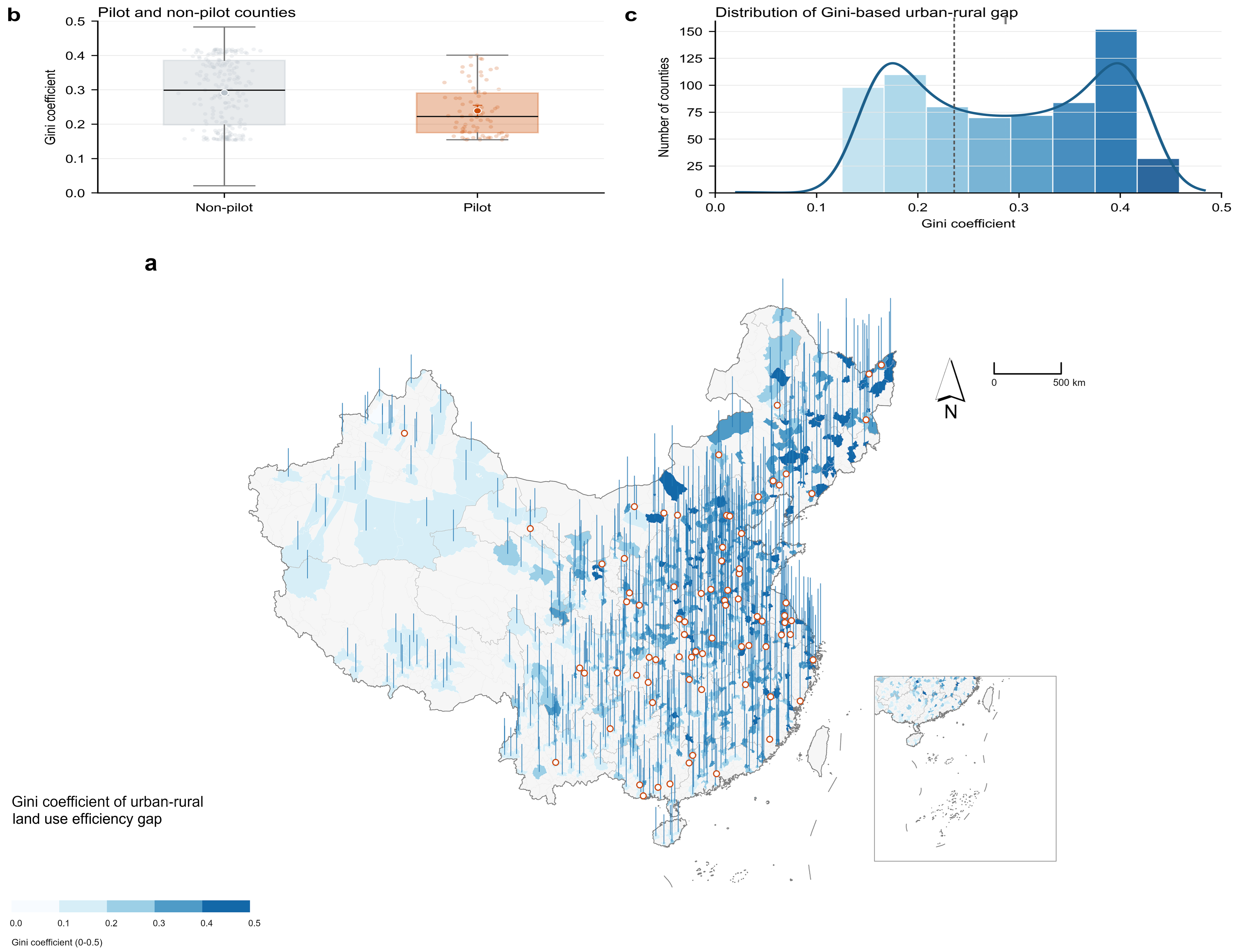
The core explanatory variable is the implementation of the Digital Agriculture Innovation and Application Base pilot program. The bases are designated and announced in successive batches by the relevant national authorities, with clearly defined county coverage and start years, so the program is treated as a quasi-natural experiment. Treat equals 1 from the year a county is included in the base list onward and 0 otherwise. Figure 2 shows the spatial distribution of the policy and of the dependent variable.

To reduce omitted-variable bias, the analysis controls for the following county characteristics: economic development, measured by the natural logarithm of GDP per capita; fiscal self-sufficiency, measured by the ratio of county fiscal revenue to fiscal expenditure; population size, measured by the natural logarithm of population density; fixed-asset investment, measured by total fixed-asset investment as a share of GDP; and urbanization, measured by the share of the urban population in the county population.

Table 1. Variable definitions and measurements.

Type	Variable	Symbol	Definition
Dependent variable	Urban–rural gap in land use efficiency	Gap	Two-group Gini coefficient constructed from urban and rural land use efficiency
Treatment variable	Policy implementation	Treat	Dummy variable equal to 1 from the year a county is designated as a Digital Agriculture Innovation and Application Base onward, and 0 otherwise
Control variable	Economic development	lnPGDP	GDP per capita (natural logarithm)
	Fiscal self-sufficiency	GOV	Fiscal revenue divided by fiscal expenditure
	Population size	lnPD	Population density (natural logarithm)
	Fixed-asset investment	INV	Total fixed-asset investment divided by GDP
	Urbanization	UR	Urban population divided by total population

reports the definitions and measurements.

Measurement and Validity of the Mechanism Variables

Agricultural technological progress (ATP) is measured as the natural logarithm of one plus the number of agricultural technology patent applications filed by entities located in the county. Patent applications in agricultural technology classes capture codified innovation output associated with the digital transformation of agriculture; respond to policy-induced research, adaptation, and application activity; and are consistently observable at the county level over the full sample period. The measure reflects innovation activity rather than farm-level adoption of specific digital devices; it does not separately identify sensors, software, algorithms, or digital decision systems, and estimates are similar when the alternative proxy, total agricultural machinery power per agricultural laborer, is used instead.

Capital misallocation (Kmis) is measured with the factor-price distortion approach of Bai and Liu [48], which builds on the aggregate-misallocation framework [5,6,7]. Within each county, the urban and rural sectors are treated as two capital-using sectors. Let s_it^R = Y_it^R/(Y_it^U + Y_it^R) denote the rural output share, β_t^U and β_t^R the sectoral output elasticities of capital estimated in Section 4.4, and ${\overline{\beta }}_{it}$ = s_it^Uβ_t^U + s_it^Rβ_t^R the output-weighted average elasticity. The rural relative distortion coefficient of the capital price is γ_it^R = [K_it^R/(K_it^U + K_it^R)]/(s_it^Rβ_t^R/${\overline{\beta }}_{it}$), which compares the actual rural capital share with the share that would be obtained if capital were allocated in proportion to output-weighted marginal products. The rural capital-misallocation index is then τ_it^R = 1/γ_it^R − 1, where positive values indicate under-allocation and negative values indicate over-allocation of capital to the rural sector relative to the efficient benchmark, and Kmis_it = |τ_it^R|, so higher values indicate more severe misallocation regardless of direction. The capital stocks, constant-price treatment, and elasticity estimation are described in Section 4.3 and Section 4.4.

Agricultural industrial upgrading (Isu) is measured as agricultural-product-processing output divided by gross agricultural output. The measure captures processing-led value-chain extension and the deepening of production–processing linkages. It does not provide a complete measure of agricultural servitization, such as digital services, technical services, logistics, or marketing services, so the empirical result is interpreted as evidence for one observable dimension of industrial upgrading rather than for the entire service-integration process.

Agricultural servitization (Aser) complements Isu on the service dimension of industrial upgrading. It is measured as the output value of agricultural, forestry, animal husbandry, and fishery services divided by the gross output value of agriculture, forestry, animal husbandry, and fishery services. The service subsector covers productive services supplied to primary production, including machinery operation, irrigation and drainage, pest and disease control, technical extension, and related outsourced services, so a rising share indicates deepening service-based integration of agricultural production. Together, Isu and Aser capture the processing-led and the service-led dimensions of the industrial-upgrading channel.

4.3. Data Sources

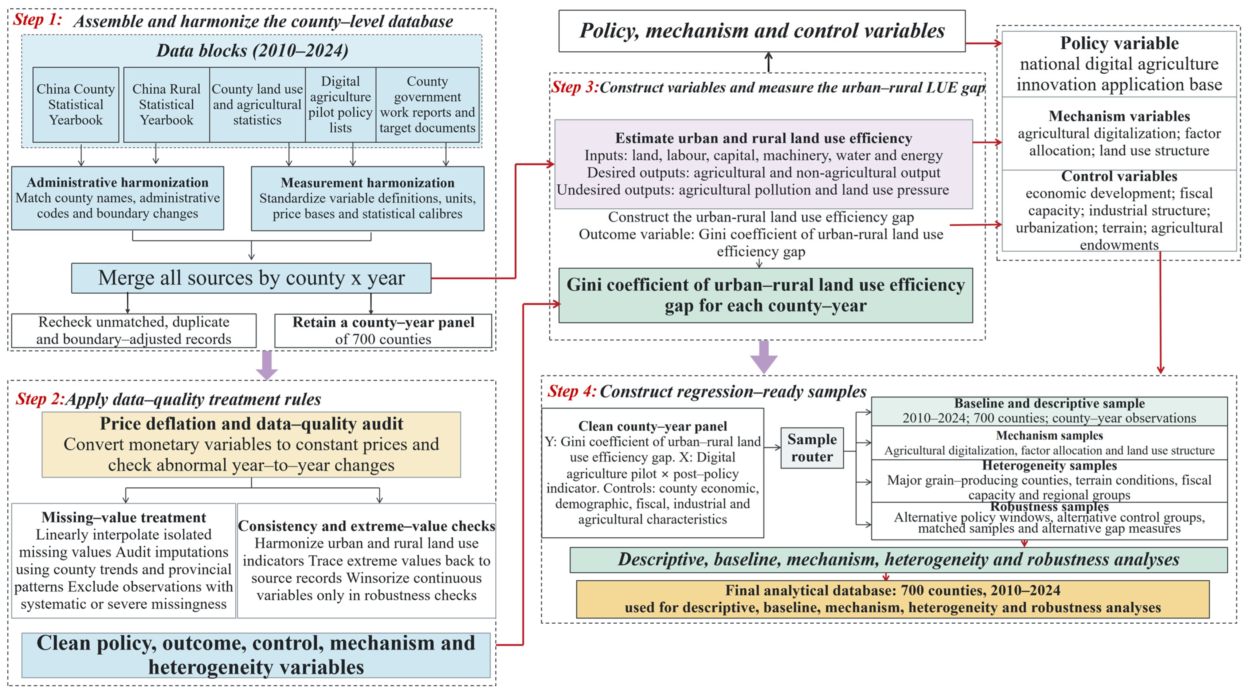
The data are drawn primarily from the China County Statistical Yearbook, the China Statistical Yearbook for Regional Economy, the China Urban–Rural Construction Statistical Yearbook, the China County Seat Construction Statistical Yearbook, and the China Statistical Yearbook.1 These are complemented by the CEIC database, the Wind Economic Database, and the China Economic and Social Big Data Research Platform.2 Land area series are compiled from annual land use change survey records and harmonized to the national land survey and land classification framework [35,49]. County statistical bulletins and official county government websites are used only to fill isolated gaps; an itemized source log is available from the corresponding author. The study period is 2010–2024. Treatment counties and start years are compiled from the national digital agriculture plan, official project notices, and the corresponding public project lists issued by the Ministry of Agriculture and Rural Affairs.3 To ensure consistency and continuity, counties with substantial missing data or major administrative-boundary adjustments are excluded. For the remaining sporadic missing values, which account for less than 5% of all observations, linear interpolation is used to complete the series, yielding a balanced county panel for the empirical analysis.

Table 2. Descriptive statistics.

Variable	Symbol	Observations	Mean	Std. Dev.	Minimum	Maximum
Urban–rural gap in land use efficiency	Gap	10,500	0.236	0.073	0.021	0.483
Digital Agriculture Innovation and Application Base pilot	Treat	10,500	0.102	0.303	0	1
GDP per capita	lnPGDP	10,500	10.485	0.634	8.748	12.036
Population size	lnPD	10,500	5.943	0.931	3.497	7.902
Fiscal self-sufficiency	GOV	10,500	0.429	0.182	0.087	0.901
Fixed-asset investment	INV	10,500	0.537	0.198	0.148	1.042
Urbanization	UR	10,500	0.509	0.147	0.192	0.887

reports the descriptive statistics, and Figure 3 summarizes the data-cleaning and sample construction process.

4.4. Construction of Marginal Return Indicators

For the extended factor-return analysis, urban output is measured by the sum of secondary- and tertiary-industry value added, with the corresponding capital stocks and employment representing urban capital and labor inputs. Rural output is measured by primary-industry value added, with agricultural capital stocks and primary-industry employment representing rural inputs. Capital stocks are constructed using the perpetual-inventory method with a depreciation rate of 9.6%, taking 2010 as the initialization year. Output and investment are converted to constant prices using their corresponding price indices. The output elasticities of capital and labor are estimated separately for the urban and rural sectors at the national sectoral level and are allowed to vary over time.

Under the Cobb–Douglas specification, the marginal return to a factor equals its estimated output elasticity multiplied by its average product. The construction is documented at the level of the depreciation rate, the initialization year, the sectoral aggregation, and the constant-price treatment; component-level deflator series and the county-specific initialization equation are not reported separately. We therefore avoid imposing an unverified additional formula and treat this remaining measurement detail as a reproducibility limitation in Section 7.3.

5. Empirical Results

5.1. Baseline Results

Table 3. Baseline regression results.

Variable	(1)	(2)
Treat	−0.016 *** (0.006)	−0.015 ** (0.007)
lnPGDP		−0.011 * (0.006)
lnPD		0.007 (0.006)
GOV		−0.014 ** (0.006)
INV		0.006 (0.005)
UR		−0.017 ** (0.008)
Constant	0.298 *** (0.008)	0.279 *** (0.037)
County fixed effects	YES	YES
Year fixed effects	YES	YES
Observations	10,500	10,500
Adjusted R2	0.641	0.663

Notes: The dependent variable is the Gini coefficient of the urban–rural gap in land use efficiency. County-clustered robust standard errors are reported in parentheses. The coefficient on Treat is the DML orthogonalized estimate; the coefficients on the controls and the constant, together with the adjusted R², are taken from an auxiliary two-way fixed-effects regression and are reported for reference. ***, **, and * denote statistical significance at the 1%, 5%, and 10% levels, respectively. The same conventions apply to all subsequent tables.

presents the baseline estimates. Column (1) includes county and year fixed effects but no controls. The policy coefficient is −0.016 and is significant at the 1% level, indicating that the program significantly lowers the Gini coefficient of urban–rural land use efficiency and narrows the gap. Column (2) adds the control variables; the coefficient remains negative and significant at the 5% level at −0.015. Relative to the sample mean of 0.236, the estimate represents a reduction of approximately 6.4%. The sign, magnitude, and statistical significance therefore support H1 and indicate an economically meaningful convergence effect.

5.2. Parallel Trends Test

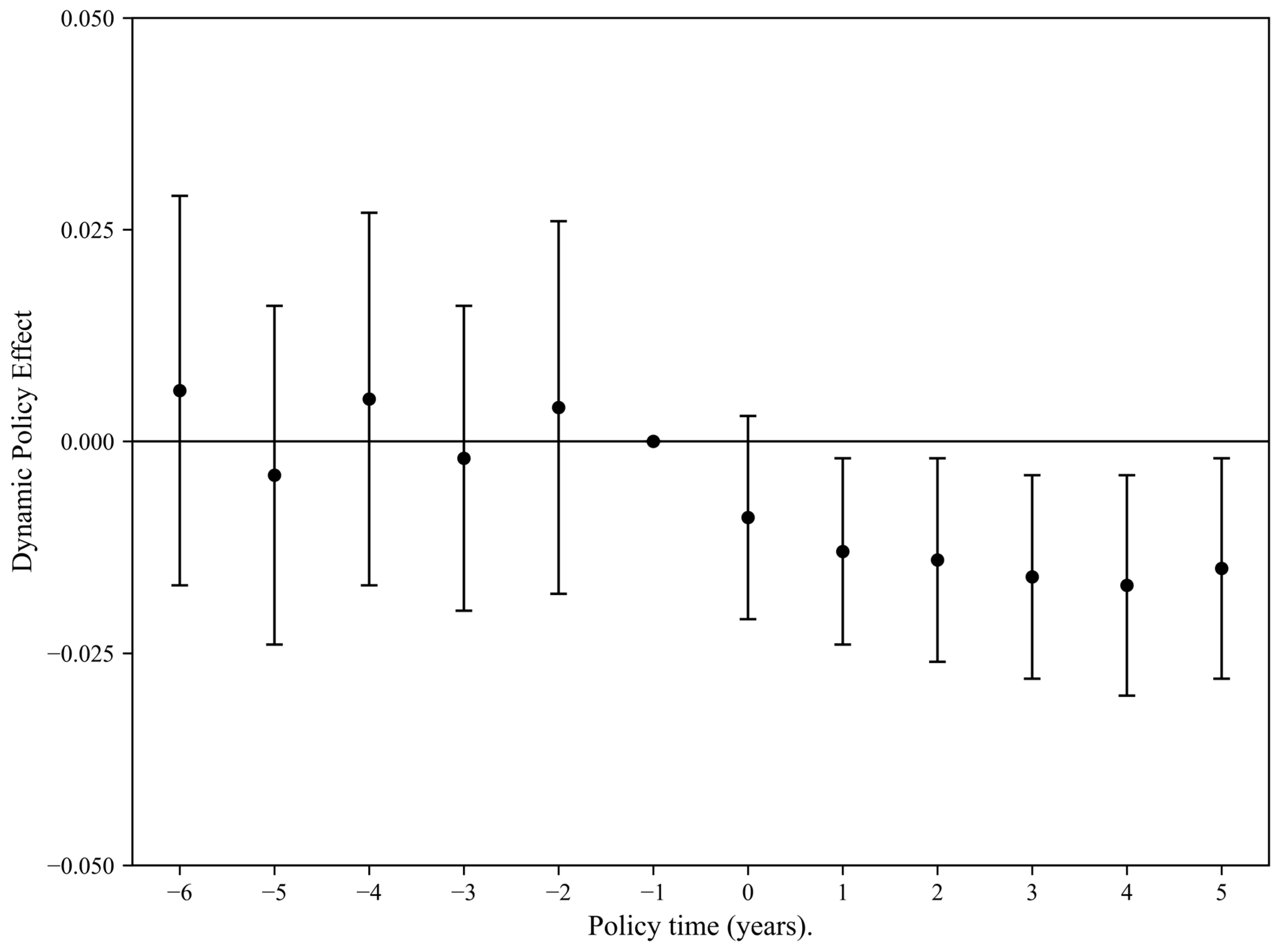
As auxiliary evidence for identification, an event-study specification is estimated within a conventional two-way fixed-effects framework. The year immediately preceding policy implementation is the reference period, and relative-time indicators are interacted with treatment status. Figure 4 reports the dynamic coefficients and confidence intervals. The pre-policy coefficients are statistically insignificant and display no systematic trend. However, because treatment begins in different years across cohorts, the TWFE dynamic coefficients are not interpreted as cohort-robust causal effects when the treatment effects may be heterogeneous [41,42]. Figure 4 is therefore used primarily as a diagnostic showing no visible differential pre-policy trend; the negative post-policy pattern is consistent with, but is not by itself the basis for, the pooled DML conclusion.

5.3. Endogeneity Test

Although DML flexibly controls for observable confounders, pilot selection may still be related to unobserved factors. The interaction between the number of fixed telephones per 10,000 people in 1984 and a time trend is therefore used as an instrument within a partially linear IV-DML framework. The time-invariant 1984 telephone measure would be absorbed by county fixed effects; interacting it with time allows the predictive relevance of historical communication infrastructure for digital agriculture adoption to evolve as digital technologies diffuse nationally. Historical fixed telephone penetration has been used in Chinese digital infrastructure research to capture path dependence in later digital adoption [39]. The relevance of this initial endowment is not assumed to be constant: interacting it with a time trend lets its predictive power for pilot designation strengthen as digital technologies diffuse nationally, which is exactly the pattern expected if early communication infrastructure confers a persistent adoption advantage, and the strong first stage below is consistent with this mechanism. At the same time, the exclusion restriction is stronger and cannot be directly tested. Historical telephone penetration may proxy for persistent development capacity, and its interaction with time could correlate with differential economic trajectories that also affect the current urban–rural land use efficiency gap. County fixed effects absorb time-invariant historical differences, year fixed effects absorb common shocks, and the DML nuisance functions flexibly condition on observed economic development, fiscal capacity, population density, investment, urbanization, and their nonlinear combinations. These controls reduce, but cannot eliminate, the remaining exclusion concern. The first-stage F statistic is 35.91, indicating that the instrument is not weak by conventional criteria, and the second-stage coefficient in

Table 4. Instrumental variable results.

Variable	(1) First Stage	(2) Second Stage
IV	0.186 *** (0.031)
Treat		−0.018 ** (0.008)
Controls	YES	YES
County fixed effects	YES	YES
Year fixed effects	YES	YES
Observations	10,500	10,500
First-stage F-statistic	35.91
Adjusted R2	0.573	0.628

Notes: The dependent variable in column (1) is Treat, and that in column (2) is Gap. IV denotes the interaction between the number of fixed telephones per 10,000 people in 1984 and a time trend. County-clustered robust standard errors are reported in parentheses. *** p < 0.01, ** p < 0.05.

remains negative and significant. Because there is one excluded instrument for one endogenous treatment variable, the specification is exactly identified, and an overidentification test is not available. A development-based second instrument cannot repair this: historical economic development measures, such as early industrial output or income levels, affect both pilot designation and the present-day urban–rural land use efficiency gap through many persistent channels, so they fail the exclusion restriction by construction and are invalid as instruments; the telephone measure is preferred precisely because its dominant persistent channel is communication infrastructure path dependence rather than general development capacity. The IV-DML estimate is therefore treated as supplementary evidence rather than as definitive proof of the exclusion restriction. A remaining concern is that early telephone penetration may also proxy for early industrialization, administrative capacity, or other persistent development conditions that can affect present urban land use efficiency outside the digital agriculture channel. The fixed effects and observed covariates reduce, but do not eliminate, this possibility. A useful extension is therefore to interact harmonized pre-policy measures of industrialization and other initial conditions with time trends when such historical county-level measures are available; in the present analysis, the IV-DML result is interpreted conservatively as supplementary evidence rather than as a standalone validation of the exclusion restriction.

5.4. Robustness Analysis

5.4.1. Alternative Machine Learning Algorithm

The random forest learner in the baseline model is replaced with LASSO. As shown in column (1) of

Table 5. Robustness tests.

Variable	(1) LASSO	(2) Alternative Dependent Variable	(3) Excluding Extreme Values	(4) Alternative Sample Period	(5) Excluding Municipal Districts	(6) Split Ratio 1:7	(7) CS-DID	(8) SA-IW
Treat	−0.014 ** (0.006)	−0.013 ** (0.006)	−0.016 ** (0.007)	−0.014 ** (0.007)	−0.015 ** (0.007)	−0.015 ** (0.006)	−0.014 ** (0.006)	−0.015 ** (0.007)
Controls	YES	YES	YES	YES	YES	YES	YES	YES
County fixed effects	YES	YES	YES	YES	YES	YES	YES	YES
Year fixed effects	YES	YES	YES	YES	YES	YES	YES	YES
Observations	10,500	10,500	10,395	7000	9300	10,500	10,500	10,500
Adjusted R2	0.663	0.612	0.681	0.657	0.668	0.663	—	—

Notes: Column (1) replaces random forests with LASSO; column (2) uses an alternative measure of the dependent variable; column (3) excludes the most extreme 1% of observations; column (4) restricts the sample to 2010–2019; column (5) excludes municipal districts; and column (6) changes the sample-splitting ratio to 1:7. County-clustered robust standard errors are reported in parentheses. ** p < 0.05. Column (3) removes 105 county-year observations, corresponding to the stated 1% trimming rule. Column (7) reports the Callaway–Sant’Anna group-time average treatment effect aggregated across cohorts and periods, and column (8) reports the Sun–Abraham interaction-weighted aggregate estimate; both use not-yet-treated and never-treated counties as comparison units, and adjusted R² is not applicable to these estimators.

, the policy coefficient is −0.014 and is significant at the 5% level, indicating that the effect does not depend on the choice of machine learning algorithm.

5.4.2. Alternative Dependent Variable

The urban component is redefined as GDP per unit of urban construction land and the rural component as the gross output value of agriculture, forestry, animal husbandry, and fisheries per unit of agricultural land. Reconstructing the gap measure with these alternatives yields a policy coefficient of −0.013 in column (2), which is significant at the 5% level, indicating robustness to the alternative measurement. Because the two-group Gini is monotone in the absolute log-ratio, the baseline index and |ln(ULE_it^U/ULE_it^R)| order urban–rural disparity equivalently. A signed ln(ULE_it^U/ULE_it^R) would answer an additional directional question rather than merely re-expressing disparity. The present robustness exercise therefore changes the economic components of the gap measure, while Section 6.2.1 addresses direction directly by estimating urban and rural land use efficiency separately. For completeness, re-estimating the baseline model with the signed log-ratio ln(ULE_it^U/ULE_it^R) as the dependent variable yields a policy coefficient of −0.078 (standard error 0.034), which is significant at the 5% level, so the conclusion does not hinge on the two-group Gini functional form.

5.4.3. Excluding Extreme Values

After excluding the most extreme 1% of observations of the gap measure (0.5% in each tail), the policy coefficient remains negative and significant at the 5% level (−0.016; column (3)), indicating that the estimate is not driven by extreme observations.

5.4.4. Placebo Test

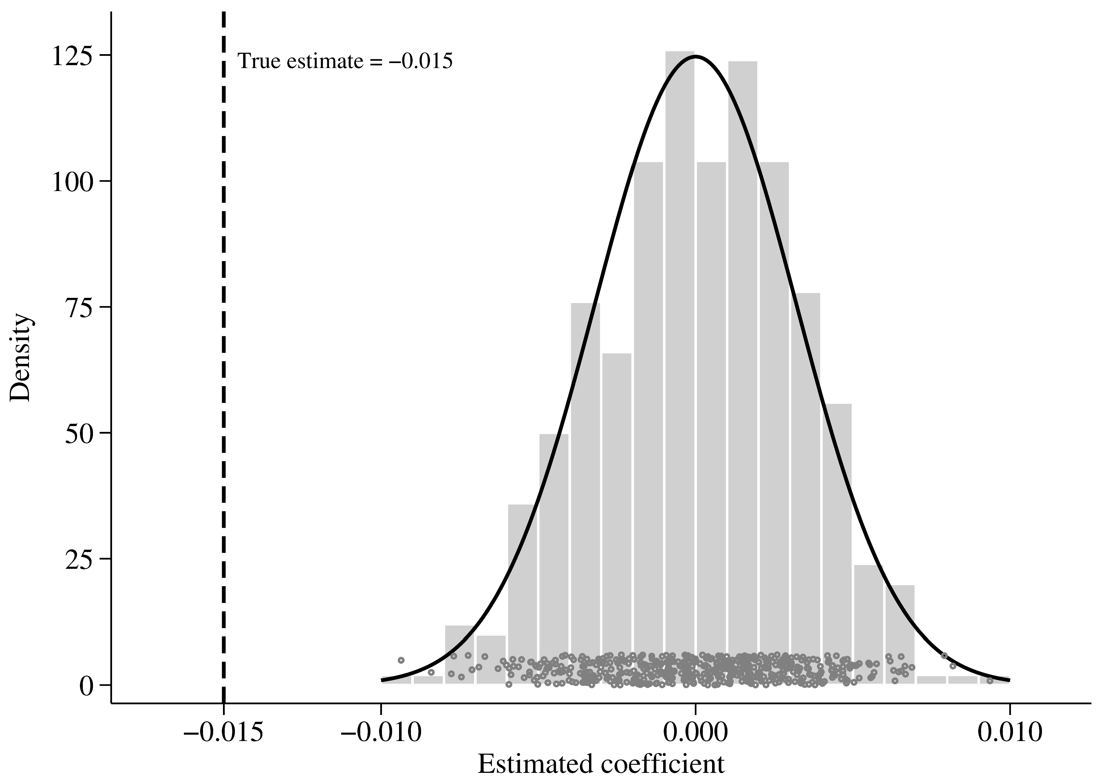
A placebo exercise randomly assigns the same number of counties as in the actual treatment group to a fictitious policy and repeats the estimation 1000 times. The mean placebo coefficient is −0.002, which is close to zero and statistically insignificant, indicating that the baseline effect is unlikely to be generated by random factors. Figure 5 presents the distribution of the placebo coefficients.

5.4.5. Alternative Sample Period

To remove potential disturbances from the COVID-19 pandemic, the model is re-estimated using only the pre-pandemic period, 2010–2019. The policy coefficient remains negative and significant at the 5% level (−0.014; column (4)), showing that the main conclusion is not driven by pandemic-related shocks.

5.4.6. Excluding Municipal Districts

Municipal districts may differ from ordinary counties in land management, urbanization, and the degree of administrative integration. Excluding them reduces the sample from 10,500 to 9300 county-year observations. Given the balanced 2010–2024 panel, this corresponds to removing 80 county-level units and retaining 620 county-level units. The policy coefficient remains negative and significant at the 5% level, indicating that the baseline result is not driven by municipal districts. This exercise is interpreted as a sensitivity check rather than a redefinition of the target population: it shifts the empirical scope toward ordinary counties, so the resulting estimate has narrower external validity. In the restricted sample, the mean of the gap measure is 0.233 with a standard deviation of 0.071, and the distributions of the control variables remain close to their full-sample counterparts.

5.4.7. Alternative Sample-Splitting Ratio

The baseline 1:4 sample split is replaced by a 1:7 split. The estimate remains negative and significant at the 5% level (−0.015; column (6)), indicating that the results are insensitive to the cross-fitting configuration.

5.5. Controlling for Concurrent Policies

To determine whether the results are affected by concurrent policies, dummy variables are constructed for four programs that may overlap with the Digital Agriculture Innovation and Application Base program—the E-Commerce into Rural Areas Comprehensive Demonstration Counties (ECRD), the Digital Village Pilot Counties (DVP), the High-Standard Farmland Construction Counties (HSF), and the Agricultural Modernization Demonstration Areas (AMD). Each dummy equals 1 from the year a county enters the corresponding policy list onward and 0 otherwise, and the dummies are added to the baseline model one at a time.

Table 6. Results after controlling for concurrent policies.

Variable	(1) +ECRD	(2) +DVP	(3) +HSF	(4) +AMD
Treat	−0.014 ** (0.006)	−0.015 ** (0.006)	−0.013 ** (0.006)	−0.016 ** (0.007)
Controls	YES	YES	YES	YES
Concurrent policy	YES	YES	YES	YES
County fixed effects	YES	YES	YES	YES
Year fixed effects	YES	YES	YES	YES
Observations	10,500	10,500	10,500	10,500
Adjusted R2	0.664	0.665	0.664	0.666

Notes: ECRD, DVP, HSF, and AMD denote E-Commerce into Rural Areas Comprehensive Demonstration Counties, Digital Village Pilot Counties, High-Standard Farmland Construction Counties, and Agricultural Modernization Demonstration Area Counties, respectively. Each column adds the corresponding policy dummy to the baseline model as an additional control. County-clustered robust standard errors are reported in parentheses. ** p < 0.05.

shows that after controlling for the ECRD, DVP, HSF, and AMD in turn, the estimated policy coefficient remains significantly negative and close to the baseline estimate, indicating that the conclusion is not materially disturbed by related concurrent policies.

5.6. Mechanism Analysis

Because ATP, Kmis, Isu, and Aser may respond to the policy, to the outcome, and to unobserved contemporaneous shocks, mechanism testing must confront the potential endogeneity of the intermediate variables; inserting them directly into the outcome equation would condition on policy-induced variation and could bias the treatment coefficient. The analysis therefore follows the three-step procedure. The first step is the baseline effect of the policy on the gap in Table 3. The second step estimates Equation (3), the effect of the policy on each mechanism variable, reported in the odd-numbered columns of

Table 7. Mechanism tests.

Variable	(1) ATP	(2) Gap	(3) Kmis	(4) Gap	(5) Isu	(6) Gap	(7) Aser	(8) Gap
Treat	0.083 ** (0.035)	−0.011 * (0.006)	−0.037 ** (0.015)	−0.010 * (0.006)	0.039 ** (0.016)	−0.011 * (0.006)	0.009 ** (0.004)	−0.012 ** (0.006)
Mechanism variable	—	−0.052 ** (0.021)	—	0.068 ** (0.027)	—	−0.044 ** (0.019)	—	−0.031 * (0.017)
Controls	YES	YES	YES	YES	YES	YES	YES	YES
County fixed effects	YES	YES	YES	YES	YES	YES	YES	YES
Year fixed effects	YES	YES	YES	YES	YES	YES	YES	YES
Observations	10,500	10,500	10,500	10,500	10,500	10,500	10,500	10,500
Adjusted R2	0.744	0.421	0.512	0.418	0.633	0.415	0.586	0.413

Notes: ATP, Kmis, Isu, and Aser denote agricultural technological progress, capital misallocation, agricultural industrial upgrading, and agricultural servitization, respectively. Odd-numbered columns report second-step regressions of each mechanism variable on the policy; even-numbered columns report third-step regressions of the gap on the policy and the corresponding mechanism variable, whose coefficient appears in the row “Mechanism variable”. County-clustered robust standard errors are reported in parentheses. * p < 0.1, ** p < 0.05.

. The third step augments the outcome equation with one mechanism variable at a time, reported in the even-numbered columns of Table 7. A significant mechanism coefficient with the expected sign, together with an attenuated policy coefficient, is consistent with partial transmission through that channel. The third step conditions on a post-treatment variable, so its mediation interpretation requires sequential ignorability, that is, no unobserved confounding between the mechanism and the outcome after conditioning on the policy, the controls, and the fixed effects; the results are read as suggestive channel evidence rather than formally identified mediation shares.

5.6.1. Agricultural Technological Progress Channel

Agricultural technological progress (ATP) is measured by the natural logarithm of one plus the number of county agricultural technology patent applications, as defined under “Measurement and Validity of the Mechanism Variables”. Column (1) of Table 7 reports a significantly positive policy coefficient, showing that smart agriculture construction is associated with an increase in agricultural innovation output. In the third-step regression in column (2), the ATP coefficient is significantly negative, and the policy coefficient is attenuated relative to the baseline, a pattern that is consistent with partial transmission through technological progress. These results support H2, subject to the sequential ignorability caveat stated above.

5.6.2. Capital Misallocation Channel

Capital misallocation (Kmis) is measured as the absolute rural capital-price distortion constructed using the Bai–Liu approach, as described under “Measurement and Validity of the Mechanism Variables”; higher values indicate a larger deviation of the rural capital share from its efficient benchmark. Column (3) of Table 7 reports a significantly negative policy coefficient, indicating that smart agriculture construction moves the county capital allocation closer to the allocation implied by sectoral marginal products. In column (4), the Kmis coefficient is significantly positive, and the policy coefficient is attenuated, consistent with partial transmission through improved capital allocation. These results support H3 under the same caveat.

5.6.3. Agricultural Industrial Upgrading Channel

Agricultural industrial upgrading (Isu) is measured by the ratio of agricultural-product-processing output to gross agricultural output and captures processing-led value-chain extension. Column (5) of Table 7 reports a significantly positive policy coefficient, and in column (6) the Isu coefficient is significantly negative with an attenuated policy coefficient, consistent with partial transmission through processing-led upgrading. These results support H4 on the processing and value-chain dimension.

5.6.4. Agricultural Servitization Channel

Agricultural servitization (Aser) is measured as the output share of agricultural, forestry, animal husbandry, and fishery services, as defined under “Measurement and Validity of the Mechanism Variables”, and captures the service-led dimension of industrial upgrading. Column (7) of Table 7 reports a significantly positive policy coefficient, indicating that smart agriculture construction deepens the service-based integration of agricultural production. In column (8), the Aser coefficient is negative and significant at the 10% level, and the policy coefficient is attenuated, consistent with a complementary service-side transmission route. Together with Isu, the evidence indicates that the industrial-upgrading channel operates through both processing-led extension and service-led integration.

6. Further Analysis

6.1. Heterogeneity Analysis

6.1.1. Heterogeneity by Poverty Status

Formerly poverty-stricken counties generally begin with weaker agricultural foundations and greater potential for rural catch-up [21,36], motivating H5c. Columns (1) and (2) of

Table 8. Heterogeneity and boundary condition analysis.

Variable	(1) Poverty-Stricken Counties	(2) Non-Poverty-Stricken Counties	(3) High Land Transfer	(4) Low Land Transfer	(5) More Taobao Villages	(6) Fewer Taobao Villages
Treat	−0.022 ** (0.009)	−0.009 (0.007)	−0.021 ** (0.009)	−0.008 (0.008)	−0.023 ** (0.009)	−0.007 (0.008)
Controls	YES	YES	YES	YES	YES	YES
County fixed effects	YES	YES	YES	YES	YES	YES
Year fixed effects	YES	YES	YES	YES	YES	YES
Observations	4245	6255	5250	5250	5250	5250
Adjusted R2	0.671	0.659	0.668	0.655	0.673	0.652
Between-group p-value	0.253		0.281		0.184

Notes: Counties are classified as formerly poverty-stricken or other counties according to whether they were formerly designated national poverty counties; as high- or low-land-transfer counties according to the sample median of the land-transfer rate; and as counties with more or fewer Taobao villages according to the sample median. Between-group p-values are obtained from Fisher permutation tests. Because all three p-values exceed 0.10, significance within one subgroup and insignificance within another should not be interpreted as a statistically significant cross-group difference. County-clustered robust standard errors are reported in parentheses. ** p < 0.05.

show a coefficient of −0.022 in formerly poverty-stricken counties, which is significant at the 5% level, and −0.009 in other counties, which is statistically insignificant. However, the Fisher permutation p-value for the between-group difference is 0.253. Therefore, the null of equal treatment effects across the two groups cannot be rejected at conventional levels. The statistically defensible conclusion is that the effect is detectable within the former-poverty group, not that the policy effect is proven to be larger than in the comparison group. H5c is thus not statistically confirmed by the between-group test.

6.1.2. Heterogeneity by Agricultural Scale Operation

Agricultural scale operation is an ex ante boundary condition because contiguous and scaled land facilitates the use of intelligent machinery and precision management [11,25,26,37], motivating H5a. Columns (3) and (4) of Table 8 report coefficients of −0.021 in the high-transfer group, which is significant at the 5% level, and −0.008 in the low-transfer group, which is statistically insignificant. The Fisher permutation p-value is 0.281, so the between-group coefficient difference is not statistically significant. The results therefore identify a within-group pattern consistent with the theoretical mechanism but do not establish that treatment effects differ across the two scale operation groups. H5a is not statistically confirmed by the formal cross-group test.

6.1.3. Heterogeneity by Digital Foundation

Digital foundations are an ex ante boundary condition because network connectivity, logistics, and digital application capacity facilitate the absorption of smart agriculture technologies [15,16,32], motivating H5b. Columns (5) and (6) of Table 8 report coefficients of −0.023 for counties with more Taobao villages, which is significant at the 5% level, and −0.007 for those with fewer, which is statistically insignificant. The Fisher permutation p-value is 0.184. Consequently, the between-group difference is not statistically significant at conventional levels. The evidence is consistent with stronger within-group detectability under better digital conditions but does not prove treatment effect heterogeneity across the two groups. H5b is not statistically confirmed by the formal cross-group test.

6.2. Extended Analysis

6.2.1. Decomposing the Urban–Rural Gap in Land Use Efficiency

To identify the source of the narrowing effect, urban land use efficiency (lnULE) and rural land use efficiency (lnRLE) are separately used as dependent variables.

Table 9. Decomposition of the urban–rural gap in land use efficiency.

Variable	(1) lnULE	(2) lnRLE
Treat	0.006 (0.031)	0.089 ** (0.038)
Controls	YES	YES
County fixed effects	YES	YES
Year fixed effects	YES	YES
Observations	10,500	10,500
Adjusted R2	0.716	0.594

Notes: lnULE and lnRLE denote the natural logarithms of urban and rural land use efficiency, respectively. County-clustered robust standard errors are reported in parentheses. ** p < 0.05.

shows that the program significantly increases rural land use efficiency but has no statistically significant effect on urban land use efficiency. The narrowing of the gap therefore comes primarily from improved rural efficiency rather than declining urban efficiency, indicating that smart agriculture construction narrows the urban–rural gap mainly by raising the agricultural output of rural land.

6.2.2. Urban–Rural Gaps in the Marginal Returns to Capital and Labor

The decomposition above shows that the program raises rural land use efficiency but does not significantly affect urban land use efficiency. Section 4.4 describes the construction of the marginal return indicators. The factor-return analysis is used to assess whether the same rural-side adjustment is accompanied by a narrowing of urban–rural factor-price signals. The mechanism variables in Section 5.6 characterize changes in technology and allocation structure, whereas the marginal return indicators characterize factor-price signals; the two analyses are complementary rather than duplicative.

To avoid duplicating the methodological details, the Cobb–Douglas specification, sectoral output and input definitions, capital-stock construction, price treatment, and estimation level for output elasticities are reported in Section 4.4. This subsection focuses on the empirical interpretation of the resulting marginal return indicators.

Following the measurement of the gap in land use efficiency, Gini coefficients are constructed from the relative differences between urban and rural marginal returns to capital (KGini) and labor (LGini); higher values indicate wider urban–rural gaps.

Table 10. Marginal returns to capital and labor in urban and rural areas.

Variable	(1) KGini	(2) LGini	(3) UMPK	(4) RMPK	(5) UMPL	(6) RMPL
Treat	−0.014 **	−0.012 **	0.007	0.092 **	0.005	0.086 **
	(0.006)	(0.005)	(0.024)	(0.039)	(0.022)	(0.037)
Controls	YES	YES	YES	YES	YES	YES
County fixed effects	YES	YES	YES	YES	YES	YES
Year fixed effects	YES	YES	YES	YES	YES	YES
Observations	10,500	10,500	10,500	10,500	10,500	10,500
Adjusted R2	0.637	0.621	0.586	0.548	0.579	0.536

Notes: KGini and LGini denote the Gini coefficients of urban–rural inequality in the marginal returns to capital and labor, respectively. UMPK and RMPK denote the marginal returns to capital in urban and rural areas; UMPL and RMPL denote the marginal returns to labor in urban and rural areas. County-clustered robust standard errors are reported in parentheses. ** p < 0.05.

reports significantly negative coefficients for both Gini measures. The logical connection runs through allocative efficiency: under the Cobb–Douglas technology of Section 4.4, a factor’s marginal return equals its output elasticity multiplied by its average product, so higher rural output per unit of land and higher rural marginal returns are two observable faces of the same rural-side adjustment, and movement of factor rewards toward the cross-sector equalization benchmark is the defining condition of efficient allocation [5,6,7]. The urban–rural gap in land use efficiency remains the dependent variable of this study; the marginal return gaps are auxiliary outcomes that corroborate the factor allocation content of the main result rather than competing outcome measures. The urban marginal returns to capital and labor are statistically unchanged, whereas the corresponding rural returns increase significantly. In an allocation interpretation, closer marginal returns are consistent with reduced factor misallocation: better matching of capital and labor with rural land can raise the productivity of rural inputs and can thereby contribute to higher rural land use efficiency. However, the current regressions do not establish a causal sequence in which equalization of factor marginal returns formally mediates the policy effect on the gap in land use efficiency. The factor-return results are therefore treated as complementary evidence on rural-side adjustment rather than as an identified underlying mediator.

7. Conclusions and Policy Implications

7.1. Conclusions

Using panel data for 700 Chinese counties from 2010 to 2024 and a double machine learning framework, this study examines the effect of smart agriculture construction on the urban–rural gap in land use efficiency and reaches three conclusions. First, smart agriculture construction significantly lowers the two-group Gini coefficient and narrows the urban–rural land use efficiency gap. Decomposition shows that the change is driven primarily by higher rural land use efficiency rather than lower urban land use efficiency, supporting the rural catch-up interpretation of H1. Second, the policy is associated with agricultural technological upgrading, lower capital misallocation, and agricultural industrial upgrading. These channels are theoretically complementary, but the mechanism regressions do not identify mediation shares or permit a quantitative ranking of relative importance. Third, within-group estimates are statistically detectable in former poverty counties, high-land-transfer counties, and counties with stronger digital foundations, but Fisher permutation tests do not establish statistically significant cross-group differences. The marginal return analysis similarly shows higher rural capital and labor returns and narrower urban–rural return gaps while urban returns remain statistically stable; these findings provide complementary allocation evidence rather than proof of a causal mediation sequence. This rural-side technology response is consistent with micro-level evidence that digital economy exposure and digital technology adoption can facilitate ecological technology adoption and technological innovation in agricultural production [50,51]. The rural catch-up pattern is consistent with international evidence that the returns to digital agriculture depend on farm scale, complementary infrastructure, advisory capacity, and the ability to finance and use new technologies [11,12,14,15,16,17,19]. The national pilot architecture and collective land institutions are specific to China, but the identified adoption constraints and complementarity conditions have broader relevance for digital agriculture and land-policy research.

7.2. Policy Implications

First, smart agriculture construction should be advanced on a sustained basis to consolidate the technological foundation for narrowing the urban–rural gap in land use efficiency. Building on the experience of the Digital Agriculture Innovation and Application Bases, policy coverage should be expanded in an orderly manner, and the application of the Internet of Things, big data, and intelligent equipment in agricultural production should be accelerated to raise the precision and intensity of rural land use, creating favorable conditions for narrowing the gap.

Second, complementary mechanisms are needed to convert smart agriculture construction into better factor allocation. Because the narrowing effect operates mainly through agricultural technological progress, the correction of capital misallocation, and agricultural industrial upgrading, the promotion of digital applications should be coordinated with stronger agricultural technology extension and talent cultivation, improved financial support and land use safeguards for capital entering rural areas, and platforms for agricultural processing, cold-chain logistics, and digital agriculture services, so that technology, capital, and industry agglomerate rationally in rural areas and rural land is used intensively and efficiently.

Third, implementation should be adapted to county agricultural and digital conditions, but the heterogeneity results should guide diagnostic attention rather than rigid targeting because the formal Fisher tests do not establish significant cross-group treatment effect differences. Counties with weaker digital infrastructure or fragmented operation may require basic connectivity, shared equipment, and service capacity, while counties with stronger foundations can deepen data integration and value-chain applications. Across settings, the priority should remain the release of rural productive potential, which is the empirically identified source of urban–rural convergence.

Beyond China, policy transferability should therefore be treated as conditional. Similar digital agriculture programs are more likely to raise rural land productivity where land use or operating rights are sufficiently secure to support investment, fragmented plots can be consolidated or served through shared-service arrangements, rural broadband and data infrastructure are reliable, and farmers have access to finance, extension, and technical support [12,15,16,17,21,23,24,25,29,30]. Where these complements are weak, fixed costs and coordination requirements can limit adoption and productivity gains. The Chinese evidence should therefore be read as evidence on a conditional mechanism—digital technology releasing underused rural productive potential—rather than as a universally transportable policy effect.

7.3. Research Limitations

Several limitations delimit the interpretation of the findings. First, data availability constrains variable measurement. Urban and rural land use efficiency are output-to-land ratios and do not incorporate land quality, undesirable outputs, ecosystem services, or the full set of production inputs; ATP captures agricultural patenting activity rather than farm-level adoption of specific digital devices; Kmis relies on estimated sectoral output elasticities; and Isu and Aser capture the processing and service dimensions of industrial upgrading rather than its finer components. The capital-stock construction is documented at the available methodological level, but more granular project, adoption, initialization, and price-deflator information would improve reproducibility. Second, DML flexibly controls for observed high-dimensional covariates but does not by itself resolve every identification issue created by staggered treatment timing and heterogeneous effects. The baseline parameter is pooled, whereas the conventional TWFE event study is used only as an auxiliary diagnostic; future work with sufficiently detailed cohort information could complement the analysis with cohort-specific staggered-DiD estimators. Unobserved selection and the IV exclusion restriction also remain potential concerns. Third, the three-step mechanism tests the condition on post-treatment mediators and therefore rests on sequential ignorability; they are read as suggestive channel evidence rather than formal mediation shares, and the factor-return analysis does not establish a causal mediation sequence. Finally, the empirical setting is a Chinese county-level digital agriculture pilot embedded in China’s land institutions, agricultural organization, fiscal system, and digital infrastructure. Generalizing the findings to other countries or institutional settings therefore requires caution. Future research could also strengthen the historical instrument design by adding harmonized pre-policy industrialization and other initial condition measures interacted with time trends, thereby testing more directly whether the telephone-based instrument proxies for persistent development trajectories.

References

1. Kendall, H.; Clark, B.; Li, W.; Jin, S.; Jones, G.D.; Chen, J.; Taylor, J.; Li, Z.; Frewer, L.J. Precision Agriculture Technology Adoption: A Qualitative Study of Small-Scale Commercial “Family Farms” Located in the North China Plain. Precis. Agric. 2022, 23, 319–351. [Google Scholar] [CrossRef] [Scilit]
2. Sun, Y.; Miao, Y.; Xie, Z.; Wu, R. Drivers and Barriers to Digital Transformation in Agriculture: An Evolutionary Game Analysis Based on the Experience of China. Agric. Syst. 2024, 221, 104136. [Google Scholar] [CrossRef] [Scilit]
3. Zhu, J.; Liu, W.; Zheng, S.; Sun, Y. Unraveling Drivers of Land Use Efficiency in Rapidly Urbanizing Areas: A Hybrid SBM-DDF and Explainable Machine Learning Framework. Habitat Int. 2025, 164, 103518. [Google Scholar] [CrossRef] [Scilit]
4. Zhang, J.; Zhang, W. The Impact Mechanism of Digital Rural Construction on Land Use Efficiency: Evidence from 255 Cities in China. Sustainability 2025, 17, 45. [Google Scholar] [CrossRef] [Scilit]
5. Hsieh, C.-T.; Klenow, P.J. Misallocation and Manufacturing TFP in China and India. Q. J. Econ. 2009, 124, 1403–1448. [Google Scholar] [CrossRef] [Scilit]
6. Restuccia, D.; Rogerson, R. The Causes and Costs of Misallocation. J. Econ. Perspect. 2017, 31, 151–174. [Google Scholar] [CrossRef] [Scilit]
7. Adamopoulos, T.; Brandt, L.; Leight, J.; Restuccia, D. Misallocation, Selection, and Productivity: A Quantitative Analysis with Panel Data from China. Econometrica 2022, 90, 1261–1282. [Google Scholar] [CrossRef] [Scilit]
8. Zhou, X.; Li, X.; Gu, X. How Does Urban–Rural Capital Flow Affect Rural Reconstruction near Metropolitan Areas? Evidence from Shanghai, China. Land 2023, 12, 620. [Google Scholar] [CrossRef] [Scilit]
9. Klerkx, L.; Jakku, E.; Labarthe, P. A Review of Social Science on Digital Agriculture, Smart Farming and Agriculture 4.0: New Contributions and a Future Research Agenda. NJAS—Wagening. J. Life Sci. 2019, 90–91, 1–16. [Google Scholar] [CrossRef] [Scilit]
10. Wolfert, S.; Ge, L.; Verdouw, C.; Bogaardt, M.J. Big Data in Smart Farming—A Review. Agric. Syst. 2017, 153, 69–80. [Google Scholar] [CrossRef] [Scilit]
11. Barnes, A.P.; Soto, I.; Eory, V.; Beck, B.; Balafoutis, A.; Sánchez, B.; Vangeyte, J.; Fountas, S.; van der Wal, T.; Gómez-Barbero, M. Exploring the Adoption of Precision Agricultural Technologies: A Cross Regional Study of EU Farmers. Land Use Policy 2019, 80, 163–174. [Google Scholar] [CrossRef] [Scilit]
12. Blasch, J.; van der Kroon, B.; van Beukering, P.; Munster, R.; Fabiani, S.; Nino, P.; Vanino, S. Farmer Preferences for Adopting Precision Farming Technologies: A Case Study from Italy. Eur. Rev. Agric. Econ. 2022, 49, 33–81. [Google Scholar] [CrossRef] [Scilit]
13. DeLay, N.D.; Thompson, N.M.; Mintert, J.R. Precision Agriculture Technology Adoption and Technical Efficiency. J. Agric. Econ. 2022, 73, 195–219. [Google Scholar] [CrossRef] [Scilit]
14. McFadden, J.; Njuki, E.; Griffin, T. Precision Agriculture in the Digital Era: Recent Adoption on U.S. Farms; Economic Information Bulletin No. 248; U.S. Department of Agriculture, Economic Research Service: Washington, DC, USA, 2023. Available online: https://www.ers.usda.gov/publications/105893 (accessed on 7 August 2026).
15. Smidt, H.J.; Jokonya, O. Factors Affecting Digital Technology Adoption by Small-Scale Farmers in Agriculture Value Chains (AVCs) in South Africa. Inf. Technol. Dev. 2022, 28, 558–584. [Google Scholar] [CrossRef] [Scilit]
16. Choruma, D.J.; Dirwai, T.L.; Mutenje, M.J.; Mustafa, M.; Chimonyo, V.G.P.; Jacobs-Mata, I.; Mabhaudhi, T. Digitalisation in Agriculture: A Scoping Review of Technologies in Practice, Challenges, and Opportunities for Smallholder Farmers in Sub-Saharan Africa. J. Agric. Food Res. 2024, 18, 101286. [Google Scholar] [CrossRef] [Scilit]
17. Cole, S.A.; Fernando, A.N. ‘Mobile’izing Agricultural Advice: Technology Adoption, Diffusion and Sustainability. Econ. J. 2021, 131, 192–219. [Google Scholar] [CrossRef] [Scilit]
18. Balafoutis, A.; Beck, B.; Fountas, S.; Vangeyte, J.; van der Wal, T.; Soto, I.; Gómez-Barbero, M.; Barnes, A.P.; Eory, V. Precision Agriculture Technologies Positively Contributing to GHG Emissions Mitigation, Farm Productivity and Economics. Sustainability 2017, 9, 1339. [Google Scholar] [CrossRef] [Scilit]
19. Walter, A.; Finger, R.; Huber, R.; Buchmann, N. Smart Farming Is Key to Developing Sustainable Agriculture. Proc. Natl. Acad. Sci. USA 2017, 114, 6148–6150. [Google Scholar] [CrossRef] [Scilit] [PubMed]
20. Finger, R.; Swinton, S.M.; El Benni, N.; Walter, A. Precision Farming at the Nexus of Agricultural Production and the Environment. Annu. Rev. Resour. Econ. 2019, 11, 313–335. [Google Scholar] [CrossRef] [Scilit]
21. Deichmann, U.; Goyal, A.; Mishra, D. Will Digital Technologies Transform Agriculture in Developing Countries? Agric. Econ. 2016, 47, 21–33. [Google Scholar] [CrossRef] [Scilit]
22. Fabregas, R.; Kremer, M.; Schilbach, F. Realizing the Potential of Digital Development: The Case of Agricultural Advice. Science 2019, 366, eaay3038. [Google Scholar] [CrossRef] [Scilit] [PubMed]
23. Ayre, M.; Mc Collum, V.; Waters, W.; Samson, P.; Curro, A.; Nettle, R.; Paschen, J.-A.; King, B.; Reichelt, N. Supporting and Practising Digital Innovation with Advisers in Smart Farming. NJAS—Wagening. J. Life Sci. 2019, 90–91, 1–12. [Google Scholar] [CrossRef] [Scilit]
24. Fielke, S.; Taylor, B.; Jakku, E. Digitalisation of Agricultural Knowledge and Advice Networks: A State-of-the-Art Review. Agric. Syst. 2020, 180, 102763. [Google Scholar] [CrossRef] [Scilit]
25. Mizik, T. How Can Precision Farming Work on a Small Scale? A Systematic Literature Review. Precis. Agric. 2023, 24, 384–406. [Google Scholar] [CrossRef] [Scilit]
26. Adamopoulos, T.; Restuccia, D. The Size Distribution of Farms and International Productivity Differences. Am. Econ. Rev. 2014, 104, 1667–1697. [Google Scholar] [CrossRef] [Scilit]
27. Rotz, S.; Duncan, E.; Small, M.; Botschner, J.; Dara, R.; Mosby, I.; Reed, M.; Fraser, E.D.G. The Politics of Digital Agricultural Technologies: A Preliminary Review. Sociol. Rural. 2019, 59, 203–229. [Google Scholar] [CrossRef] [Scilit]
28. Eastwood, C.; Klerkx, L.; Ayre, M.; Dela Rue, B. Managing Socio-Ethical Challenges in the Development of Smart Farming: From a Fragmented to a Comprehensive Approach for Responsible Research and Innovation. J. Agric. Environ. Ethics 2019, 32, 741–768. [Google Scholar] [CrossRef] [Scilit]
29. Shepherd, M.; Turner, J.A.; Small, B.; Wheeler, D. Priorities for Science to Overcome Hurdles Thwarting the Full Promise of the ‘Digital Agriculture’ Revolution. J. Sci. Food Agric. 2020, 100, 5083–5092. [Google Scholar] [CrossRef] [Scilit] [PubMed]
30. Finger, R. Digital Innovations for Sustainable and Resilient Agricultural Systems. Eur. Rev. Agric. Econ. 2023, 50, 1277–1309. [Google Scholar] [CrossRef] [Scilit]
31. Zhang, J.; Zhang, W. Harnessing Digital Technologies for Rural Industrial Integration: A Pathway to Sustainable Growth. Systems 2024, 12, 564. [Google Scholar] [CrossRef] [Scilit]
32. Qiao, C. Coupling Digital Inclusive Finance and Rural E-Commerce: A Systems Perspective on China’s Urban–Rural Income Gap. Systems 2025, 13, 911. [Google Scholar] [CrossRef] [Scilit]
33. Standing Committee of the National People’s Congress of the People’s Republic of China. Land Administration Law of the People’s Republic of China (2019 Amendment); Standing Committee of the National People’s Congress of the People’s Republic of China: Beijing, China, 2019. Available online: https://www.mee.gov.cn/ywgz/fgbz/fl/201904/t20190428_701293.shtml (accessed on 8 August 2026). (In Chinese)
34. Ministry of Agriculture and Rural Affairs of the People’s Republic of China. Measures for the Administration of the Transfer of Rural Land Management Rights; Ministry of Agriculture and Rural Affairs Order No. 1 of 2021; Ministry of Agriculture and Rural Affairs of the People’s Republic of China: Beijing, China, 2021. Available online: https://www.moj.gov.cn/pub/sfbgw/flfggz/flfggzbmgz/202104/t20210422_357846.html (accessed on 8 August 2026). (In Chinese)
35. GB/T 21010-2017; Current Land Use Classification. General Administration of Quality Supervision, Inspection and Quarantine of the People’s Republic of China, Standards Press of China: Beijing, China, 2017. Available online: https://openstd.samr.gov.cn/bzgk/std/newGbInfo?hcno=224BF9DA69F053DA22AC758AAAADEEAA (accessed on 8 August 2026).
36. National Bureau of Statistics of China. Income of Rural Residents in Poor Areas in the First Quarter of 2020. 2020. Available online: https://www.stats.gov.cn/english/PressRelease/202005/t20200505_1742976.html (accessed on 8 August 2026).
37. Xu, D.; Liu, Y.; Li, Y.; Liu, S.; Liu, G. Effect of Farmland Scale on Agricultural Green Production Technology Adoption: Evidence from Rice Farmers in Jiangsu Province, China. Land Use Policy 2024, 147, 107381. [Google Scholar] [CrossRef] [Scilit]
38. Li, X.; Shi, X.; Qin, Y. Exploring the Effects of Farmland Transfer on Farm Household Well-Being: Evidence from Ore–Agriculture Compound Areas in Northwest China. Land 2024, 13, 2042. [Google Scholar] [CrossRef] [Scilit]
39. Dong, H.; Tao, M.; Wang, J.; Baiocchi, G. How Broadband Infrastructure Development Impacts Green Innovation? A Corporate Financialization Mediated Perspective. Sustain. Dev. 2024, 32, 6881–6902. [Google Scholar] [CrossRef] [Scilit]
40. Chernozhukov, V.; Chetverikov, D.; Demirer, M.; Duflo, E.; Hansen, C.; Newey, W.; Robins, J. Double/Debiased Machine Learning for Treatment and Structural Parameters. Econom. J. 2018, 21, C1–C68. [Google Scholar] [CrossRef] [Scilit]
41. Sun, L.; Abraham, S. Estimating Dynamic Treatment Effects in Event Studies with Heterogeneous Treatment Effects. J. Econom. 2021, 225, 175–199. [Google Scholar] [CrossRef] [Scilit]
42. Callaway, B.; Sant’Anna, P.H.C. Difference-in-Differences with Multiple Time Periods. J. Econom. 2021, 225, 200–230. [Google Scholar] [CrossRef] [Scilit]
43. Lu, X.; Wang, M.; Tang, Y. The Spatial Changes of Transportation Infrastructure and Its Threshold Effects on Urban Land Use Efficiency: Evidence from China. Land 2021, 10, 346. [Google Scholar] [CrossRef] [Scilit]
44. Sicular, T.; Yue, X.; Gustafsson, B.; Li, S. The Urban–Rural Income Gap and Inequality in China. Rev. Income Wealth 2007, 53, 93–126. [Google Scholar] [CrossRef] [Scilit]
45. Cowell, F.A. Measuring Inequality, 3rd ed.; Oxford University Press: Oxford, UK, 2011. [Google Scholar]
46. Zhong, C.; Peng, L.; Yu, J.; Swan, I.; Li, H. Toward More Reliable, Complete, and Equitable Global Urban Land Use Efficiency Assessments. Commun. Earth Environ. 2025, 6, 1055. [Google Scholar] [CrossRef] [Scilit]
47. Melchiorri, M.; Pesaresi, M.; Florczyk, A.J.; Corbane, C.; Kemper, T. Principles and Applications of the Global Human Settlement Layer as Baseline for the Land Use Efficiency Indicator—SDG 11.3.1. ISPRS Int. J. Geo-Inf. 2019, 8, 96. [Google Scholar] [CrossRef] [Scilit]
48. Bai, J.H.; Liu, Y.Y. Can Outward Foreign Direct Investment Improve the Resource Misallocation of China? China Ind. Econ. 2018, 1, 60–78. (In Chinese) [Google Scholar] [CrossRef]
49. TD/T 1055-2019; Technical Regulation of the Third Nationwide Land Survey. Ministry of Natural Resources of the People’s Republic of China, Geological Publishing House: Beijing, China, 2019.
50. Yang, C.; Ji, X.; Cheng, C.; Liao, S.; Obuobi, B.; Zhang, Y. Digital Economy Empowers Sustainable Agriculture: Implications for Farmers’ Adoption of Ecological Agricultural Technologies. Ecol. Indic. 2024, 159, 111723. [Google Scholar] [CrossRef] [Scilit]
51. Wang, W.; Huang, Z.; Fu, Z.; Jia, L.; Li, Q.; Song, J. Impact of Digital Technology Adoption on Technological Innovation in Grain Production. J. Innov. Knowl. 2024, 9, 100520. [Google Scholar] [CrossRef] [Scilit]
Figure 1. Theoretical framework of how smart agriculture construction narrows the urban–rural gap in land use efficiency. The three central channels are complementary and potentially mutually reinforcing. The upper boxes summarize the ex ante boundary-condition hypotheses, whereas the lower boxes indicate that the Fisher permutation tests do not establish statistically significant cross-group differences in treatment effects.
Land 15 01531 g001
Figure 2. Spatial distribution of the smart agriculture pilot policy and the urban–rural gap in land use efficiency. Notes: The map is based on the 2024 standard map service system of China (approval number GS(2024)0650) published by the Ministry of Natural Resources; the base map is unmodified and is used for academic presentation only. Panel (a) shows the spatial distribution of the urban–rural gap in land use efficiency across the 700 sample counties in 2020. County fill colors and column heights both represent the Gini coefficient of the gap, which ranges from 0 to 0.5 with a sample mean of 0.236 and a standard deviation of 0.073; darker colors and taller columns indicate a wider gap. Ring markers denote counties designated as national Digital Agriculture Innovation and Application Bases, and the inset in the lower right shows the South China Sea islands in full. Panel (b) compares the raw distributions of the Gini coefficient in pilot and non-pilot counties using box plots and individual observations; no regression estimate is overlaid on the box plot. The baseline DML estimate is −0.015 and is reported here only for reference, not as the raw pilot–non-pilot difference. Panel (c) shows the distribution of the gap across the 700 counties; bars denote county frequencies, the solid line is a kernel density estimate, and the vertical dashed line marks the sample mean (0.236).
Land 15 01531 g002
Figure 3. Data cleaning, variable construction, and sample formation.
Land 15 01531 g003
Figure 4. Dynamic effects of the Digital Agriculture Innovation and Application Base pilot program.
Land 15 01531 g004
Figure 5. Distribution of coefficients from the placebo test.
Land 15 01531 g005