Research on the Dynamic Response of Urban Blue–Green–Grey Space Trade-Off/Synergy and Waterlogging Disaster Risks

Abstract

The layout of urban blue, green and grey spaces plays a crucial role in flood risk, but the potential trade-offs and synergistic effects of these spaces on urban flood risk have not been fully studied. This research uses the spatial Durbin model to analyze the direct impact of changes in urban blue, green and grey spaces on risk changes and the spatial spillover effects, revealing how the balance and coordination states and their changes affect urban flood risk. The results show the following: (1) An increase in the balance effect is often accompanied by an increase in risk, but there are differences in the intensity and direction of response at different stages, and the risk changes show significant spatial dependence and spillover effects. (3) The analysis of the spatial Durbin model indicates that the increase in blue and green spaces mainly alleviates risks through local retention and storage. It is notable that in the later stage, the neighborhood spillover effect of green spaces has exceeded its direct local effect, highlighting the collaborative value of green network connectivity at the regional level; while the impact of grey spaces is the most complex—although the construction of sponge cities and urban rainwater management have led to a negative direct local effect (2020–2024), its positive neighborhood spillover effect still persists. Clearly understanding how “balance and coordination” affects risk at different development stages can help urban managers formulate differentiated strategies for the proportion of blue, green and grey spaces based on the development stage of the city, thereby avoiding the use of “one-size-fits-all” planning standards.

1. Introduction

Urban flooding caused by heavy rainfall is a typical urban disaster resulting from the combined effects of global climate change and rapid urbanization [1]. Every year, more than 100 cities at or above the county level in China are hit by urban flooding, and the recent frequent occurrence of heavy rainfall events has further exacerbated the risk of such disasters [2]. According to statistics, approximately two-thirds of China’s land area is at risk of flooding, and more than two-thirds of its cities have experienced relatively severe flooding. Examples include the “21 July” extreme rainstorm in Beijing in 2012 and the “20 July” extreme rainstorm in Zhengzhou in 2021, both of which resulted in significant property damage and loss of life [3].

Currently, China’s extreme weather events are exacerbating urban waterlogging problems [4], while the rapid urbanization process has increased impermeable surfaces, significantly altering hydrological response processes in urban environments [5,6,7,8]. Taking the extreme rainstorm in Guangzhou as an example, relevant studies have examined the spatiotemporal distribution patterns, evolution processes and formation mechanisms of urban surface flooding in relation to drainage system capacity, as well as corresponding disaster mitigation strategies [9]. The combined effect of extreme rainfall and insufficient drainage capacity may significantly exacerbate the potential economic and social consequences of floods [10,11,12]. Against the backdrop of rapid urbanization, urban waterlogging has become one of the most prominent challenges for public welfare and sustainable development [13,14]. Since 2006, more than 100 cities in China have experienced urban waterlogging each year [15]. China has taken measures such as formulating disaster prevention and mitigation plans, establishing disaster reduction centers and building sponge cities to effectively reduce the impact of urban flooding disasters. However, in extreme circumstances, these measures can still cause significant losses. Improving the infrastructure and landscape can help alleviate the risk of water accumulation [16]. However, the traditional “mainly relying on drainage” concept for flood prevention is no longer sufficient to cope with the complexity and uncertainty presented by the urban water system under the dual influence of intense human activities and climate change [17]. Therefore, it is urgent to explore new, more resilient and adaptable approaches for urban flood control from the perspective of coordinated regulation of infrastructure [18]. Urban infrastructure refers to the basic facilities that maintain the normal operation of a city, including drainage systems, water supply systems, transportation networks and power facilities. These infrastructures not only provide the fundamental guarantee for urban development and residents’ lives, but also play a crucial role in responding to urban flood risks [19]: (1) Blue infrastructure refers to spaces where water is an important ecological element, including lakes, rivers and constructed urban water landscapes, which provide significant psychological and recreational benefits due to human proximity to water [20,21]. (2) Green infrastructure refers to an ecosystem network constructed on the carrier of various green spaces, including small-scale facilities such as rain gardens and green roofs, as well as natural spaces at the catchment scale such as forests and grasslands, as well as elements such as parks and green streets in cities [22,23,24]. (3) Grey infrastructure refers to build-up and impermeable infrastructure [25,26,27]. In rapidly urbanizing areas, the expansion of impervious surfaces is widely recognized as a major driver of increased surface runoff and heightened flood risks [28,29]. Impermeable areas reduce infiltration capacity and increase direct runoff, leading to higher peak flows and shorter lag times. In contrast, green and blue infrastructure—such as vegetation, open water bodies and nature-based drainage systems—can mitigate flood risks by increasing infiltration, enhancing water storage capacity and delaying runoff responses [30]. Consequently, the hydrological behavior of urban systems depends not only on the proportion of different land cover types but also on their spatial arrangement—the latter determining the connectivity and interactions of runoff pathways [31].

Currently, a large number of studies have systematically analyzed the mechanism and effectiveness of the role of different types of infrastructure in mitigating urban waterlogging risks; With a consensus indicating that a combined blue–green–grey infrastructure strategy is superior to single infrastructure solutions [32,33,34], some scholars have developed a cost–benefit performance model to assess the cooling effect of green and blue spaces in the Beijing area [35], especially with green and blue infrastructure being considered one of the most effective natural climate adaptation measures to mitigate urban heat islands [36,37,38]. Existing research has confirmed that grey infrastructure, green infrastructure and topography are the main factors affecting the city’s ability to cope with waterlogging, and most of the research focuses on exploring the optimal configuration and function of grey and green infrastructure [39,40,41]. To meet the needs of multifunctional spaces, scholars have developed an integrated assessment framework for the multifunctional potential and cost of blue–green infrastructure, providing a scientific basis for high-density cities to prioritize cost-effective, optimized blue–green infrastructure [42]. Orak et al. proposed a systematic method based on Bayesian networks to evaluate and prioritize mixed infrastructure solutions that integrate blue–green and grey infrastructure [43]. Gomes et al. verified in the Brazilian basin that the combination of blue–green infrastructure and grey facilities can enhance land value and environmental quality index, highlighting the economic feasibility of synergistic benefits [44]. When some facilities are located in areas prone to flooding, improving connectivity can significantly reduce local flooding [45]. Constructing and optimizing the BGI network can alter the runoff pathways within the watershed and the patterns of water flow into rivers and lakes, significantly changing the key input parameters of the lake water resource balance model [46]; this has thereby enhanced surface drainage and improved the hydrological connectivity of the runoff pathways within the watershed [47]. It is noteworthy that related research has further proposed trade-offs and synergistic benefits of different types of infrastructure in improving waterlogging management [48]; The relevant research employed the backward planning method, taking into account land-use change scenarios and CCS, and optimizing the spatial configuration of the traditional, cost-intensive grey infrastructure (GREI) and the rapidly developing green infrastructure (GI) integration [49]. However, relatively little attention has been paid to how the spatial distribution of urban land cover components and their interactions influence hydrological responses and flood risk dynamics. In particular, the potential trade-off and synergy among grey, green and blue surfaces in regulating runoff have not been fully explored, especially at the microscale.

Furthermore, due to the interdependence of hydrological processes, the risk of urban flooding exhibits significant spatial dependence [50]. Runoff generated in a given area can propagate outward through drainage networks and surface channels, leading to a spatial spillover effect on waterlogging disaster risk. Traditional analytical methods often overlooked such spatial interactions, which may result in biased estimates of the impact of urban land-use changes. Combining spatial econometric methods with data-driven models can help better capture the local and neighboring effects of urban surface on waterlogging disaster risk.

Regarding the evolution of the relationship between urban blue, green, and grey spaces, scholars have traced the historical progression of infrastructure spatial configuration from a phase dominated by “grey infrastructure” through the emergence of “green infrastructure” to the “integration of green and grey infrastructure” [51,52]. The current research mainly focuses on the temporal and spatial evolution characteristics and driving mechanisms of blue–green spaces and blue–green–grey areas [53,54]. Existing research has focused on the spatiotemporal evolution characteristics and driving mechanisms of blue–green and blue–green–grey areas, among other aspects. Current research indicates that urban land use patterns and infrastructure directly influence urban flood risk by altering surface runoff pathways, drainage efficiency and stormwater retention capacity [55]. Significant progress has been made in existing research on the differentiated impacts of the three types of infrastructure. A study by Wang et al., which used an extreme precipitation index to fit a flood risk function for Beijing, showed that the impact of the three types of infrastructure on flood risk, in order of magnitude, is green infrastructure > grey infrastructure > blue infrastructure [56]. Under extreme rainfall conditions, performance differences among various types of infrastructure become even more pronounced; the three categories of infrastructure should be evaluated through a comprehensive and optimized approach. The “top-support effect” of blue infrastructure reflects the importance of its hydraulic connections and coupling relationships [57,58]. With regard to quantitative research on synergistic effects, findings indicate that not all blue–green–grey combinations produce synergistic effects; the mechanisms of interaction between facilities are key to determining the extent of these effects [59].

Domestic and international research on the balance and coordination of urban blue, green and grey spaces mainly focuses on the coordination of two types of elements. The research mainly concentrates on three fields: ecological environment, economic benefits and human health. In terms of ecological services, researchers have proposed an ecological logic for the integration of blue and green spaces, emphasizing the need to enhance system efficiency by reconfiguring the ecological order [60]. In the study on the temporal and spatial evolution of carbon storage in urban blue, green and grey spaces in Henan Province, China from 2000 to 2020, the relationship between the changes in urban blue, green and grey spaces and carbon storage under four scenarios in the next 20 years was simulated [61]. Guo et al. systematically integrated 82 global studies to investigate the response patterns of birds with different habitat preferences to the characteristics of urban green spaces. They found that vegetation complexity and grey space would interfere with bird diversity [62]. In terms of economic benefits, scholars have proposed a dual-performance model that balances ecological benefits and economic benefits to optimize the layout of urban green spaces and enhance the comprehensive functions of urban green spaces [63]. In terms of human health, Potter et al. explored the impact of urban blue, green and grey spaces on human health, and studied biodiversity, microbial communities and their relationship with the environment [64]. The results showed that human activities encroaching on the natural environment led to ecological imbalance, which in turn affected health. The research methods concerning the coordination of urban blue, green and grey spaces focus on the integration of multiple disciplines and empirical analysis. Based on the InVEST model and correlation analysis, scholars studied the trade-off/collaborative effects of the blue and green infrastructure ecosystem services in Wuhan at three different scales: administrative districts, townships and streets, and river basin units [65].

The comprehensive analysis of existing studies reveals that although considerable progress has been made in researching the relationship between urban blue, green and grey spaces and urban flood risk, the following deficiencies still exist. Most of the existing studies focus on the disaster mitigation effects of blue and green infrastructure and the optimization of their spatial layout, but pay insufficient attention to the dynamic changes of blue, green and grey spaces during urban expansion. The blue, green and grey space layout of the city often exhibit a structural reorganization of this kind of interdependence, which may either form a mutually reinforcing synergy or trigger a trade-off effect due to space occupation, pattern fragmentation and decreased connectivity, thereby having a phased impact on the flood risk pattern and risk changes. This study is the first to extend the trade-off-cooperation theory from the relationship of ecosystem services to the configuration relationship between urban blue, green and grey spaces. It constructs a framework for evaluating the trade-off and cooperation between blue, green and grey spaces, thereby overcoming the limitations of traditional methods that only focus on the correlation of single variables or static assessment. Moreover, by integrating spatial scales and temporal dynamics, this indicator can more accurately identify the dynamic response of urban flood risks to the configuration process of blue–green infrastructure. Exploring the trade-off/cooperation effects of urban blue–green–grey spaces and their spatial optimization configuration strategies to enhance the city’s ability to prevent flood disasters has become a key research direction in urban stormwater management.

2. Research Area, Data Sources, and Evaluation Index System

2.1. Research Area

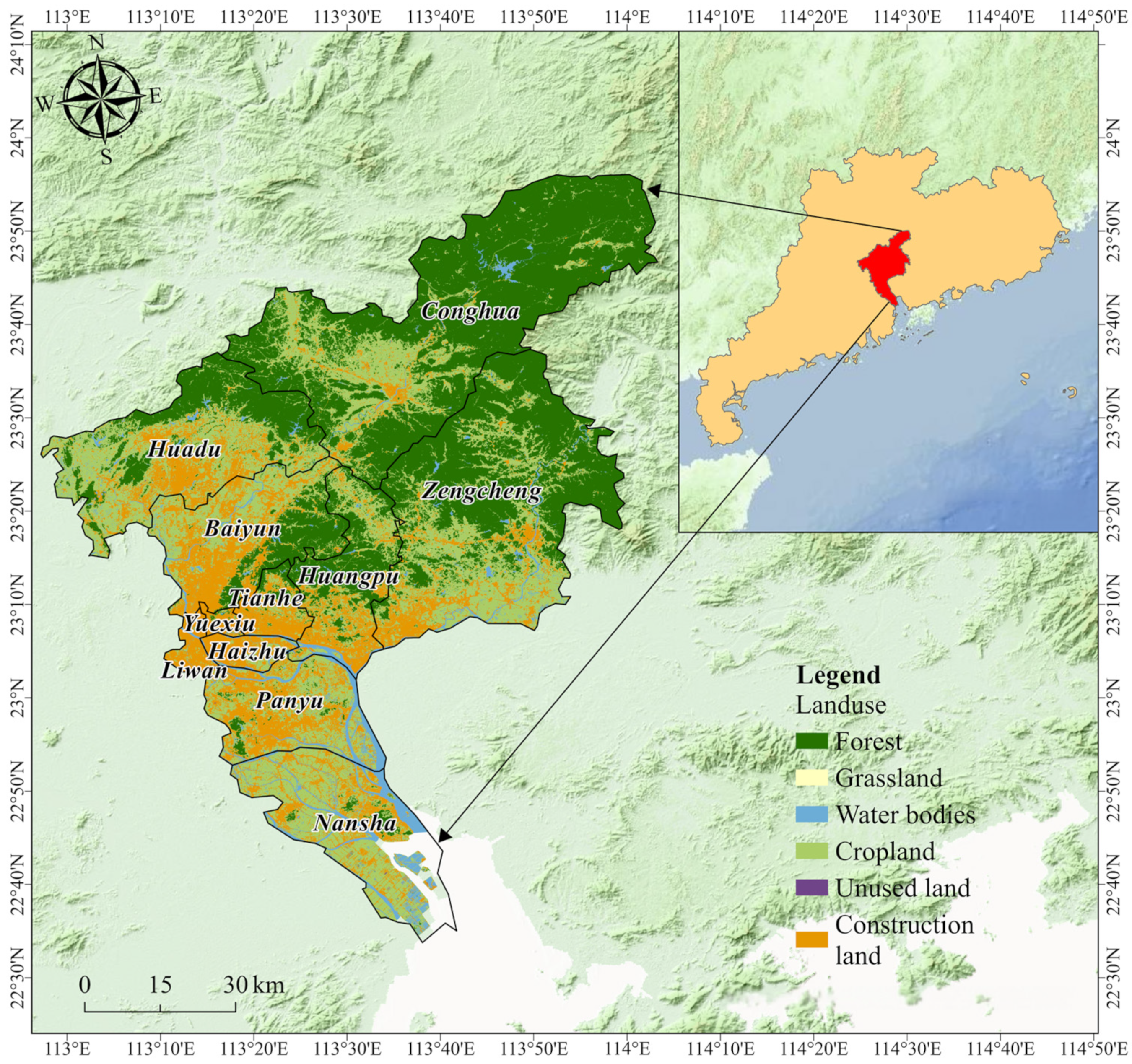
As the core node of the Guangdong–Hong Kong–Macau Greater Bay Area and the political center of Guangdong Province (Figure 1), Guangzhou bears multiple functions as a national central city, an international comprehensive hub, a commercial and technological innovation center and a historical and cultural city. Its administrative jurisdiction covers a total area of 7434.4 km², including 11 districts, including Yuexiu, Haizhu and Liwan. As shown in Figure 1, due to its location in the heart of the Pearl River Delta and the influence of terrain and climate, the region is densely covered with rivers and has a developed water system, making it a typical delta network river area. In recent years, Guangzhou has frequently experienced severe rain waterlogging events. For example, the major rainstorms in 2017 (“5·7”), 2018 (“6·8”), 2019 (“6·13”), 2020 (“5·22” and “6·7”) and 2025 (“8·2”) resulted in six severe rainstorms. Due to the complex nature of urban waterlogging, which is influenced by natural climate, terrain, urbanization and many other factors, the problem is extremely complex and difficult to manage. It is imperative to accurately diagnose the current situation and problems of waterlogging prevention and control in Guangzhou. The low standards of water and pipeline systems and insufficient drainage capacity; therefore, the risk management of waterlogging disasters in Guangzhou is urgent.

2.2. Data Sources and Data Processing

This study constructs an index system for flood risk (

Table 1. Waterlogging disaster risk evaluation index system.

Target Layer	Indicator Layer	Sub-Index Level	Hierarchical Analysis Method	Weight Entropy Weight Method	Combination	Property	Reference
Urban waterlogging Disaster Risk Index	Risk (0.335)	C1 Heavy Rainfall Days (days)	0.3280	0.2092	0.2756	(+)	[66]
		C2 waterlogging season rainfall (mm)	0.6720	0.7908	0.7244	(+)	[67]
	Sensitivity (0.290)	Elevation (m)	0.4070	0.0100	0.3090	(−)	[67]
		Slope (°)	0.1830	0.0191	0.1425	(−)	[66]
		Vegetation Coverage (%)	0.1100	0.0982	0.1071	(−)	[68]
		River network density (km/km2)	0.3000	0.8727	0.4414	(+)	[67]
	Vulnerability (0.270)	Per capita GDP (10,000 yuan/km2)	0.1890	0.3561	0.2604	(+)	[67]
		Population Density (people/km2)	0.4930	0.4178	0.4608	(+)	[67]
		Building Density (km2/km2)	0.3180	0.2262	0.2787	(+)	[66]
	Disaster Prevention and Mitigation Capacity (0.105)	Government Public Budget (Billion Yuan)	0.2380	0.7753	0.3719	(−)	[67]
		Drainage pipeline density (km/km2)	0.6080	0.1518	0.4943	(−)	[67]
		Healthcare institution beds per 10,000 people (units)	0.1540	0.0729	0.1338	(−)	[67]

“+” and “−” indicate that the indicator is positive and negative, respectively.

). Heavy rainfall days: Data were sourced from the “China Meteorological Data Network.” Daily precipitation data from weather stations in the study area were selected to calculate the number of heavy rain days (

Table A1. Weather station information.

Year	Weather Station Name	Latitude	Longitude	Number of Valid Observations Recorded
2010	LAU FAU SHAN, CH	22.4666666	113.9833333	183
	CHEUNG CHAU, CH	22.2	114.0166666	183
	HUIMIN, CH	37.5	117.5333333	180
	TAI SHAN, CH	36.25	117.1	182
	HUILI, CH	26.65	102.25	181
	HUIZE, CH	26.4	103.25	180
	MACHENG, CH	31.1333333	114.95	183
	SHAOGUAN, CH	24.6666666	113.6	182
	FOGANG, CH	23.8833333	113.5166666	183
	LIANPING, CH	24.3666666	114.4833333	183
	GAOYAO, CH	23.05	112.4666666	181
	BAIYUN INTERNATIONAL, CH	23.392436	113.298786	174
	BAOAN INTERNATIONAL, CH	22.639258	113.810664	177
	SHANGCHUAN DAO, CH	21.7333333	112.7666666	182
2015	LAU FAU SHAN, CH	22.4666666	113.9833333	183
	CHEUNG CHAU, CH	22.2	114.0166666	183
	TAI SHAN, CH	36.25	117.1	183
	MACHENG, CH	31.1333333	114.95	183
	LIANPING, CH	24.3666666	114.4833333	183
	SHAOGUAN, CH	24.6666666	113.6	180
	FOGANG, CH	23.8833333	113.5166666	183
	LIANPING, CH	24.3666666	114.4833333	183
	GAOYAO, CH	23.05	112.4666666	181
	BAIYUN INTERNATIONAL, CH	23.392436	113.298786	168
	BAOAN INTERNATIONAL, CH	22.639258	113.810664	173
	SHANGCHUAN DAO, CH	21.7333333	112.7666666	183
2020	LAU FAU SHAN, CH	22.4666666	113.9833333	183
	CHEUNG CHAU, CH	22.2	114.0166666	179
	TAI SHAN, CH	36.25	117.1	183
	MACHENG, CH	31.1333333	114.95	183
	LIANZHOU, CH	24.8	112.3666666	183
	SHAOGUAN, CH	24.6666666	113.6	183
	FOGANG, CH	23.8833333	113.5166666	183
	LIANPING, CH	24.3666666	114.4833333	182
	GAOYAO, CH	23.05	112.4666666	178
	BAIYUN INTERNATIONAL, CH	23.392436	113.298786	183
	BAOAN INTERNATIONAL, CH	22.639258	113.810664	110
	SHANGCHUAN DAO, CH	21.7333333	112.7666666	183
2024	LAU FAU SHAN, CH	22.4666666	113.9833333	177
	CHEUNG CHAU, CH	22.2	114.0166666	179
	HUIMIN, CH	37.5	117.5333333	180
	TAI SHAN, CH	36.25	117.1	173
	HUIZE, CH	26.4	103.25	172
	MACHENG, CH	31.1333333	114.95	176
	SHAOGUAN, CH	24.6666666	113.6	178
	FOGANG, CH	23.8833333	113.5166666	179
	LIANPING, CH	24.3666666	114.4833333	179
	GAOYAO, CH	23.05	112.4666666	179
	BAIYUN INTERNATIONAL, CH	23.392436	113.298786	179
	BAOAN INTERNATIONAL, CH	22.639258	113.810664	181
	SHANGCHUAN DAO, CH	21.7333333	112.7666666	178

). The specific processing procedure was as follows: ① Collect data from weather stations in Guangzhou and calculate the number of heavy rain days at each station based on China’s meteorological classification standards: Number of heavy rain days = number of days within the year with daily precipitation ≥50 mm. ② Quality control: Remove outliers, such as missing values and invalid codes (e.g., 999.9, 99.99). ③ Calculate the number of heavy rainfall days by year: Tally the number of days with daily precipitation ≥50 mm for each meteorological station from 2010 to 2024. Use ordinary Kriging interpolation in ArcGIS Pro3.7 to interpolate the data from the meteorological stations and generate a raster of heavy rainfall days. ④ Calculate the root mean square error (RMSE) for leave-one-out cross-validation (LOOCV): Estimate the RMSE using the Geostatistics Wizard analysis.

Waterlogging season rainfall (mm): The annual average rainfall during the flood season is defined as the summation of the cumulative rainfall during the flood period (from April to September) within the study period. ① Using data from weather stations, calculate the cumulative rainfall for the annual flood season based on daily rainfall records. ② In ArcGIS Pro, use ordinary Kriging interpolation to interpolate data from the weather stations and generate a raster of the number of days with heavy rainfall. ③ Calculate the root mean square error (RMSE) for leave-one-out cross-validation (LOOCV): estimate the RMSE in the Geostatistics Wizard analysis.

Elevation data: Sourced from the Geospatial Data Cloud (https://www.gscloud.cn/); spatial resolution converted to 1 km via resampling; slope data: derived from elevation data using slope analysis in ArcGIS; vegetation cover data: sourced from the National Qinghai–Tibet Plateau Scientific Data Center; spatial resolution was converted to 1 km via resampling; River Network Density Data: the data are sourced from the National Basic Geographic Information Database. Using ArcGIS10.8 software, the river vector data were processed through; per capita GDP data: data sourced from the Guangzhou Statistical Yearbook; population density data: data sourced from the Guangzhou Statistical Yearbook; building density data: data sourced from OpenStreetMap’s full-featured geographic data; government general budget data: data sourced from the Guangzhou Statistical Yearbook; Drainage pipeline density data: data sourced from Guangzhou municipal facility statistics; Healthcare institution beds per 10,000 people: data sourced from the Guangzhou Statistical Yearbook.

The land use data were obtained from the China Land Use Remote Sensing Monitoring Dataset maintained by the Resource and Environmental Science Data Center (RESDC) of the Chinese Academy of Sciences. To ensure consistency in spatial scale across multiple data sources, all land-use raster data were resampled to a spatial resolution of 1 km. First, the land use data were uniformly projected into the WGS 1984 UTM coordinate system and cropped to the study area. Subsequently, based on the study objectives, the original land-use types were reclassified into built-up areas, cropland, forested land, water bodies, grassland and unutilized land. Blue spaces: water bodies such as rivers and lakes; green spaces: ecological spaces such as forested land and grassland; grey spaces: built-up areas and unutilized land.

3. Research Methods

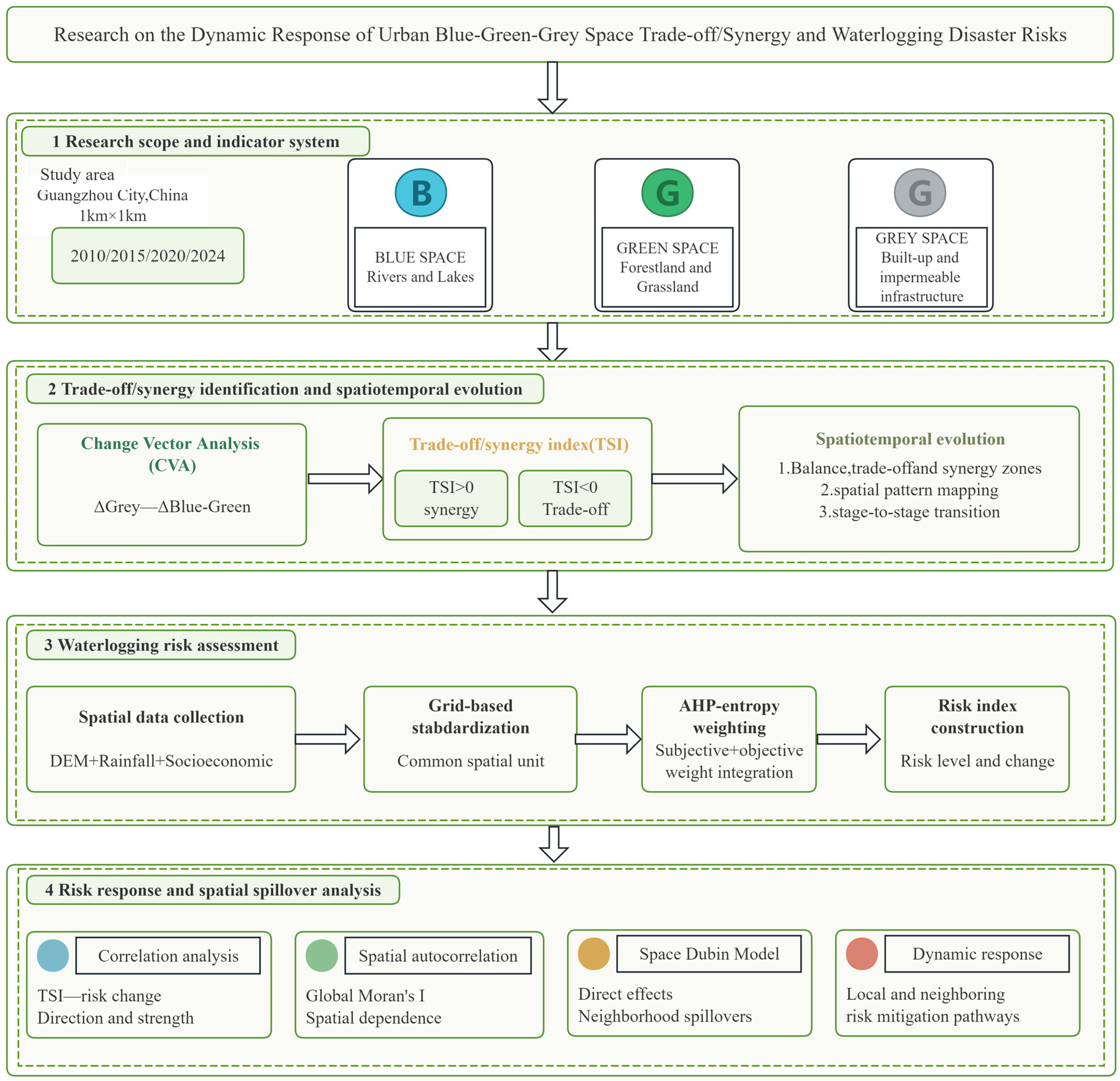
The overall framework of this study is as follows (Figure 2): (1) quantitatively characterize the trade-offs and synergies among urban blue, green and grey spaces and map their spatiotemporal evolution; (2) assess urban flood risk patterns across multiple time periods and measure their dynamic changes; (3) analyze the impact of changes in trade-offs and synergies among urban blue, green and grey spaces on urban flooding risk.

3.1. Urban Blue–Green–Grey Space Trade-Off/Synergy Research Method

Drawing on the trade-off/synergy framework in ecosystem service research [69] and the urban grey–green scale coordination index [70], and combining the needs of urban waterlogging management, this paper defines the trade-off/synergy of urban blue–green–grey spaces as follows:

Synergy: The change in blue–green space can match or exceed the change in grey space. For example, when grey expands, blue–green synchronously increases or decreases only slightly, or when grey retreats, blue–green can recover/increase, indicating that urban development and ecological regulation functions are relatively coordinated. Trade-off: The change in grey space is significantly better than the change in blue–green space. For example, when grey rapidly expands, blue–green significantly shrinks, or when the compensation for blue–green is insufficient to match the grey increment, it is at the expense of ecological space for construction expansion, and the regulatory capacity tends to weaken.

Change Vector Analysis (CVA)

This paper uses a 1 km × 1 km regular grid as the basic analysis unit and sets the study period from t₁ to t₂. Let A be the area of the corresponding element within the grid (unit: km²), and the blue space, green space and grey space are denoted as B, G and Grey, respectively. Define the change amount of the grey space and the change amount of the blue–green space:

$$\Delta \mathrm{Grey} = {\mathrm{A}}_{\mathrm{Grey},{\mathrm{t}}_2}-{\mathrm{A}}_{\mathrm{Grey},{\mathrm{t}}_1}$$

(1)

$$\Delta \mathrm{BG}=({\mathrm{A}}_{\mathrm{B},{\mathrm{t}}_2}+{\mathrm{A}}_{\mathrm{G},{\mathrm{t}}_2})-({\mathrm{A}}_{\mathrm{B},{\mathrm{t}}_1}+{\mathrm{A}}_{\mathrm{G},{\mathrm{t}}_1})$$

(2)

Accordingly, the change in blue–green–grey in grid units over [${\mathrm{t}}_1$, ${\mathrm{t}}_2$] can be represented as a two-dimensional point ($\Delta \mathrm{Grey}$, $\Delta \mathrm{BG}$). The “direction” of the vector is used to identify the type of synergy/compensation, and the “magnitude” of the vector is used to measure the intensity of the change.

The direction angle $\mathsf{\theta }$ of the change vector is calculated using the four-quadrant arctangent function:

$$\mathsf{\theta } = \mathrm{atan}2(\Delta \mathrm{BG}, \Delta \mathrm{Grey})$$

(3)

To unify θ to the interval [0, 2π), define

$${\mathsf{\theta }}^{*}=\{\begin{array}{ll}\mathsf{\theta }+2\mathsf{\pi }& \mathrm{if} \mathsf{\theta } < 0\\ \mathsf{\theta }& \mathrm{if} \mathsf{\theta } \ge 0\end{array}$$

(4)

With the straight line $\Delta \mathrm{BG}= \Delta \mathrm{Grey}$ (y = x, 45° direction line) as the geometric boundary, in this context, the use of 45° as the discriminant criterion in this study is not an empirical setting but is based on geometric relationships in a two-dimensional coordinate space. When constructing a coordinate system with the change in grey space ($\Delta \mathrm{Grey}$) as the x-axis and the combined change in blue–green space ($\Delta \mathrm{BG}$) as the y-axis, the line $\Delta \mathrm{BG}= \Delta \mathrm{Grey}$ (i.e., y = x) represents the equilibrium line where the magnitudes of change in the two spaces are equal. Since this line forms a 45° angle with the x-axis, the 45° angle corresponds to a geometric state in which changes in blue–green space and grey space are consistent, rather than an arbitrarily determined empirical threshold.

When a data point lies on or above the line y = x ($\Delta \mathrm{BG}$ ≥ $\Delta \mathrm{Grey}$), it indicates that the increase in blue–green space (or a smaller decrease) matches or even exceeds the change in grey space, reflecting the urban ecological space’s strong capacity to compensate for the expansion of built-up space; this is therefore defined as a “synergy” state.

Conversely, when a data point lies below y = x ($\Delta \mathrm{BG}$ < $\Delta \mathrm{Grey}$), it indicates that the expansion of grey space outpaces the improvement in blue–green space, or that the degree of blue–green space degradation exceeds the change in grey space. This suggests insufficient ecological compensation and a tendency toward imbalance in the allocation of blue–green and grey spaces; therefore, this is defined as a “Trade-off” state.

Furthermore, when $\Delta \mathrm{BG}$ = 0 and $\Delta \mathrm{Grey}$ = 0, it indicates that neither blue–green space nor grey space has changed, and the system remains in a stable state (Stable).

Therefore, 45° is not an empirical threshold but rather a discriminatory benchmark naturally determined by the geometric relationship of the two-dimensional coordinates. Based on this, the directional factor is defined:

$$\mathrm{S}=\{\begin{array}{c}+1 \mathrm{i}\mathrm{f} {\mathsf{\theta }}^{*}\in [{\displaystyle \frac{\mathsf{\pi }}{4}},{\displaystyle \frac{5\mathsf{\pi }}{4}})\\ -1 \mathrm{if} {\mathsf{\theta }}^{*}\in [0,{\displaystyle \frac{\mathsf{\pi }}{4}})\cup [{\displaystyle \frac{5\mathsf{\pi }}{4}},2\mathsf{\pi })\\ 0 \mathrm{i}\mathrm{f} \Delta \mathrm{B}\mathrm{G}=0 \mathrm{a}\mathrm{n}\mathrm{d} \Delta \mathrm{G}\mathrm{r}\mathrm{e}\mathrm{y}=0\end{array}$$

(5)

The intensity factor L takes the magnitude of the change vector (Euclidean distance):

$$\mathrm{L} = \sqrt{{(\Delta \mathrm{Grey})}^2+{(\Delta \mathrm{BG})}^2}$$

(6)

The direction factor is synthesized with the intensity factor to obtain the blue–green–grey space trade-off/collaboration index (TSI):

$$\mathrm{TSI}=\mathrm{S}\times \mathrm{L}$$

(7)

$\mathrm{TSI}$ stands for signed continuous variables (unit: km²): $\mathrm{TSI}$ > 0 indicates synergy, $\mathrm{TSI}$ < 0 indicates trade-off, $\mathrm{TSI}$ = 0 indicates no change; a higher $\left|\mathrm{TSI}\right|$ value indicates a stronger degree of synergy or trade-off.

To support the spatial zoning analysis, this paper classifies based on the continuous TSI (

Table 2. Balance/synergy strength grading.

Level	TSI Range (km2)	Waterlogging Regulation Changes
Significant synergy	TSI ≥ 0.03	Blue–green space changes significantly match or exceed grey space changes, regulating capacity is significantly improved
Intermediate synergy	0.001 ≤ TSI < 0.03	Blue–green space change matching or better than grey space change, regulating capacity slightly improved
Balance	−0.001 < TSI < 0.001	Changes are slight, in a stable or slight update range, the regulation and storage capacity is basically stable
Intermediate synergy	−0.03 < TSI ≤ −0.01	Grey space changes are relatively dominant, the regulation and storage capacity slightly decreases
Significant trade-off	TSI ≤ −0.03	Grey space changes significantly dominate or blue–green space significantly attenuates, regulating capacity is obviously weakened (key focus area)

). According to the Classification Standards for Urban Green Spaces issued by the Ministry of Housing and Urban–Rural Development of the People’s Republic of China, a discrepancy of 0.001 km² may result from statistical errors caused by grid pixels; furthermore, basic functional units of green spaces, such as neighborhood parks, typically correspond to an area of 1–5 hectares (https://www.mohurd.gov.cn/). On the other hand, the Technical Guidelines for Sponge City Construction (2014) indicate that a change of 0.03 km² in green space can result in differences in flood retention capacity, and that changes in the proportion of impervious surfaces are highly sensitive to flood peaks (https://www.gz.gov.cn/zwgk/fggw/sfbgtwj/content/mpost_9224696.html) (accessed on 20 December 2025). Taking both the planning scale and hydrological significance into account, 0.001 km² and 0.03 km² are adopted as thresholds for moderate to high-level changes.

3.2. Urban Waterlogging Disaster Risk Assessment Method

3.2.1. Weighted Sum Method

Given that urban flood risks are influenced by a combination of factors—including the natural environment, land use and socioeconomic conditions—and that each evaluation indicator possesses both clear theoretical significance and distinct data dispersion characteristics, this study employs a combined weighting method that integrates the Analytic Hierarchy Process (AHP) with the entropy weighting method. AHP can reflect the importance of indicators based on existing theories and expert knowledge, while the entropy weighting method can objectively determine weights based on the information entropy of indicators, reflecting the degree to which each indicator contributes to distinguishing differences among evaluation units and reducing human subjective bias. The combined weighting method balances theoretical understanding with data characteristics, achieving complementarity between subjective and objective weighting, and enhancing the scientific rigor and reliability of the evaluation results; therefore, it is suitable for comprehensive evaluations of urban flood risks and research on blue–green–grey spaces.

(1)

Analytic Hierarchy Process, AHP

To determine the relative importance of each indicator in the indicator system, first, based on the formation mechanism of urban flooding risk, a hierarchical model comprising the objective layer, criterion layer and indicator layer is constructed. Subsequently, using the 1–9 rating scale proposed by Saaty, pairwise comparisons were conducted among indicators at the same level to construct a judgment matrix. This judgment matrix was developed based on existing research findings on urban flooding risk assessment, the theoretical significance of the indicators and the actual conditions of the study area, and was refined by incorporating relevant domain knowledge.

This paper uses the Consistency Ratio (CR) to evaluate the validity of the judgment matrix.

$$CI={\displaystyle \frac{{\lambda }_{max}-n}{n-1}}$$

(8)

$$CR={\displaystyle \frac{CI}{RI}}$$

(9)

where ${\lambda }_{max}$ is the largest eigenvalue of the decision matrix; $n$ is the order of the matrix; $CI$ is the consistency index; $RI$ is the random consistency index. When $CR<0.10$, the decision matrix is considered to have passed the consistency test, and the results are deemed to have good consistency.

(2)

Entropy Weight Method, EWM

The entropy weight method is an objective weighting method that determines weights based on the degree of discretization of the indicator data itself [71]. The information entropy of each index is used to determine its weight.

There is an $\mathrm{m}$ evaluation index and $\mathrm{n}$ evaluation unit, and the original data matrix is $\mathrm{X} = {\left({\mathrm{x}}_{\mathrm{ij}}\right)}_{\mathrm{n}\times \mathrm{m}}$, where ${\mathrm{x}}_{\mathrm{ij}}$ represents the original value of the $i$-th evaluation unit for the $\mathrm{j}$-th index. The calculation steps of the entropy weight method are as follows:

Original data are standardized to obtain the standardized matrix $\mathrm{Z} ={\left({\mathrm{z}}_{\mathrm{ij}}\right)}_{\mathrm{n}\times \mathrm{m}}$, Calculate the weight ${\mathrm{p}}_{\mathrm{i}\mathrm{j}}$ of the $i$-th evaluation unit under the $j$-th indicator:

$${\mathrm{p}}_{\mathrm{ij}} = {\displaystyle \frac{{\mathrm{z}}_{\mathrm{ij}}}{{\displaystyle {\sum }_{\mathrm{i}=1}^{\mathrm{n}}}{\mathrm{z}}_{\mathrm{ij}}}}$$

(10)

In the formula, when ${\mathrm{z}}_{\mathrm{i}\mathrm{j}}=0$, let ${\mathrm{p}}_{\mathrm{i}\mathrm{j}}\mathrm{l}\mathrm{n}{\mathrm{p}}_{\mathrm{i}\mathrm{j}}=0$.

Calculate the information entropy ${\mathrm{H}}_{\mathrm{j}}$ of the $j$-th indicator:

$${\mathrm{H}}_{\mathrm{j}} = -{\displaystyle \frac{1}{\mathrm{lnn}}}{\displaystyle {\sum }_{\mathrm{i}=1}^{\mathrm{n}}}{\mathrm{p}}_{\mathrm{ij}}{\mathrm{lnp}}_{\mathrm{ij}}$$

(11)

In the formula, $\mathrm{n}$ represents the number of evaluation units; ${\displaystyle \frac{1}{\mathrm{l}\mathrm{n}\mathrm{n}}}$ is the normalization coefficient, used to ensure $0\le {\mathrm{H}}_{\mathrm{j}}\le 1$.

Calculate the difference coefficient of the ${\mathrm{g}}_{\mathrm{j}}$ for the $j$-th indicator:

$${\mathrm{g}}_{\mathrm{j}} = 1 - {\mathrm{H}}_{\mathrm{j}}$$

(12)

The coefficient of variation ${\mathrm{g}}_{\mathrm{j}}$ reflects the degree of variation of the data of the $j$-th indicator, the larger ${\mathrm{g}}_{\mathrm{j}}$ it is, the higher the discriminability of the indicator, and the greater its contribution to the evaluation results.

Calculate the entropy weight of the ${\mathrm{w}}_{\mathrm{j}}$ for the $j$-th indicator:

$${\mathrm{W}}_{\mathrm{j}} = {\displaystyle \frac{{\mathrm{g}}_{\mathrm{j}}}{{\displaystyle {\sum }_{\mathrm{j}=1}^{\mathrm{m}}}{\mathrm{g}}_{\mathrm{j}}}}={\displaystyle \frac{1 -{ \mathrm{H}}_{\mathrm{j}}}{{\displaystyle {\sum }_{\mathrm{j}=1}^{\mathrm{m}}}\left(1 -{ \mathrm{H}}_{\mathrm{j}}\right)}}$$

(13)

In the formula, ${\mathrm{W}}_{\mathrm{j}}$ is the entropy weight of the $i$-th indicator, satisfying $0 \le { \mathrm{W}}_{\mathrm{j}} \le 1$ and ${\displaystyle {\sum }_{\mathrm{j}=1}^{\mathrm{m}}}{\mathrm{W}}_{\mathrm{j}} = 1$.

(3)

Weighted Sum Method

In practical applications, the range transformation method is first used to preprocess the raw data in order to eliminate differences in units and values among the data points. The formula for calculating the composite weight is as follows:

$${\mathrm{w}}_{\mathrm{j}} = \mathsf{\alpha }\mathrm{w}{\prime }_{\mathrm{j}}+\mathsf{\beta }\mathrm{w}{″}_{\mathrm{j}}$$

(14)

In the formula, ${\mathrm{w}}_{\mathrm{j}}$ is the combined weight of the $j$-th indicator; $\mathrm{w}{\prime }_{\mathrm{j}}$ is the subjective weight obtained from the Analytic Hierarchy Process; $\mathrm{w}{″}_{\mathrm{j}}$ is the objective weight obtained from the Entropy Weight Method; $\mathsf{\alpha }$ and $\mathsf{\beta }$ are the weight distribution coefficients, satisfying $\mathsf{\alpha } + \mathsf{\beta } = 1$.

To coordinate the degree of difference between $\mathsf{\alpha }$ and $\mathsf{\beta }$ with the difference in subjective $\mathrm{w}{\prime }_{\mathrm{j}}$ and objective weights $\mathrm{w}{″}_{\mathrm{j}}$, this paper introduces the concept of a distance function to determine the allocation coefficient [72]. The distance between subjective and objective weights is defined as

$$\mathrm{d}\left(\mathrm{w}\prime ,\mathrm{w}″\right)=\sqrt{{\displaystyle \frac{1}{2}}{\displaystyle {\sum }_{\mathrm{j}=1}^{\mathrm{m}}}{\left(\mathrm{w}{\prime }_{\mathrm{j}}-\mathrm{w}{″}_{\mathrm{j}}\right)}^2}$$

(15)

Let the difference of the distribution coefficients $\left|\mathsf{\alpha }-\mathsf{\beta }\right|$ be equal to the weighted distance $\mathrm{d}\left(\mathrm{w}\prime , \mathrm{w}″\right)$, combine $\mathsf{\alpha } + \mathsf{\beta } = 1$, and solve to obtain:

$$\mathsf{\alpha } = {\displaystyle \frac{1+\mathrm{d}}{2}}, \mathsf{\beta } = {\displaystyle \frac{1 - \mathrm{d}}{2}} \mathrm{or} \mathsf{\alpha } = {\displaystyle \frac{1 - \mathrm{d}}{2}},\mathsf{\beta } = {\displaystyle \frac{1+\mathrm{d}}{2}}.$$

(16)

This article selects a set of distribution coefficients that yield a more reasonable combined weight based on actual calculations.

3.2.2. Urban Waterlogging Disaster Risk Assessment Model

This paper adopts geometric weighting to construct a comprehensive risk index that characterizes the “shortage effect” and the multi-dimensional coupling characteristics of the waterlogging disaster risk system.

Firstly, calculate the hazard factor risk index (H), the disaster-prone environment sensitivity index (S), the disaster-affected body vulnerability index (V) and the disaster prevention and reduction capacity index (C), and finally input the results into the urban waterlogging disaster risk assessment model (R). The formula is as follows:

$${\mathrm{H}}_{\left(\mathrm{x}\right)} = {\displaystyle {\sum }_{\mathrm{j}=1}^{\mathrm{i}}}\left[{\mathrm{w}}_{\mathrm{j}}\times {\mathrm{H}}_{\mathrm{j}\left(\mathrm{x}\right)}\right]$$

(17)

$${\mathrm{S}}_{\left(\mathrm{x}\right)}={\displaystyle {\sum }_{\mathrm{j}=1}^{\mathrm{i}}}\left[{\mathrm{w}}_{\mathrm{j}}\times {\mathrm{S}}_{\mathrm{j}\left(\mathrm{x}\right)}\right]$$

(18)

$${\mathrm{V}}_{\left(\mathrm{x}\right)}={\displaystyle {\sum }_{\mathrm{j}=1}^{\mathrm{i}}}\left[{\mathrm{w}}_{\mathrm{j}}\times {\mathrm{V}}_{\mathrm{j}\left(\mathrm{x}\right)}\right]$$

(19)

$${\mathrm{C}}_{\left(\mathrm{x}\right)}={\displaystyle {\sum }_{\mathrm{j}=1}^{\mathrm{i}}}\left[{\mathrm{w}}_{\mathrm{j}}\times {\mathrm{C}}_{\mathrm{j}\left(\mathrm{x}\right)}\right]$$

(20)

$${\mathrm{R}}_{\left(\mathrm{x}\right)}={{\mathrm{H}}_{\left(\mathrm{x}\right)}}^{{\mathrm{W}}_{\mathrm{H}}}\times {{\mathrm{S}}_{\left(\mathrm{x}\right)}}^{{\mathrm{W}}_{\mathrm{S}}}\times {{\mathrm{V}}_{\left(\mathrm{x}\right)}}^{{\mathrm{W}}_{\mathrm{V}}}\times {{\mathrm{C}}_{\left(\mathrm{x}\right)}}^{{\mathrm{W}}_{\mathrm{C}}}$$

(21)

In the formula, the evaluation unit is $\mathrm{x}$; ${\mathrm{w}}_{\mathrm{j}}$ the weight of each indicator; ${\mathrm{H}}_{\mathrm{j}\left(\mathrm{x}\right)}$, ${\mathrm{S}}_{\mathrm{j}\left(\mathrm{x}\right)}$, ${\mathrm{V}}_{\mathrm{j}\left(\mathrm{x}\right)}$, ${\mathrm{C}}_{\mathrm{j}\left(\mathrm{x}\right)}$ are the standardized values of each indicator; ${\mathrm{R}}_{\left(\mathrm{x}\right)}$ is the comprehensive risk index of waterlogging disaster for the evaluation unit $\mathrm{x}$; ${\mathrm{W}}_{\mathrm{H}}$, ${\mathrm{W}}_{\mathrm{S}}$, ${\mathrm{W}}_{\mathrm{V}}$, ${\mathrm{W}}_{\mathrm{C}}$ are the criterion layer weights of the four factors, respectively.

To identify the changes in the risk of urban waterlogging for subsequent effects, the spatial distribution maps for the risk changes of urban waterlogging in Guangzhou during the three periods of 2010–2015, 2015–2020 and 2020–2024 were drawn. A positive change value indicates an increase in the risk of urban waterlogging during that period, a negative value indicates a decrease in risk and the larger the absolute value, the more dramatic the change.

$${\Delta \mathrm{R}}_{\mathrm{i}} ({\mathrm{t}}_1\to {\mathrm{t}}_2)={\mathrm{R}}_{\mathrm{i}} \left({\mathrm{t}}_2\right)-{\mathrm{R}}_{\mathrm{i}}\left({\mathrm{t}}_1\right)$$

(22)

In the formula, ${\Delta \mathrm{R}}_{\mathrm{i}}({\mathrm{t}}_1\to {\mathrm{t}}_2)$ represents the incremental increase in waterlogging disaster risk between ${\mathrm{t}}_1$ − ${\mathrm{t}}_2$.

3.3. Response Process Analysis Method

3.3.1. Correlation Analysis

Examining the degree of correlation between two or more variables that are non-normal or have unknown distributions, the calculation formula is as follows:

$$\mathsf{\rho } = 1 - {\displaystyle \frac{6{\displaystyle {\sum }_{\mathrm{i}=1}^{\mathrm{n}}}{\mathrm{d}}_{\mathrm{i}}^2}{\mathrm{n}\left({\mathrm{n}}^2-1\right)}}$$

(23)

$${\mathrm{d}}_{\mathrm{i}}=\mathrm{R}({\mathrm{x}}_{\mathrm{i}})-\mathrm{R}({\mathrm{y}}_{\mathrm{i}})$$

(24)

In the formula, $\mathsf{\rho }$ is the rank correlation coefficient; $\mathrm{R}\left({\mathrm{x}}_{\mathrm{i}}\right)$ and $\mathrm{R}\left({\mathrm{y}}_{\mathrm{i}}\right)$ are the ranks of ${\mathrm{x}}_{\mathrm{i}}$ and ${\mathrm{y}}_{\mathrm{i}}$, respectively; ${\mathrm{d}}_{\mathrm{i}}$ is the sorted position; n is the number of 1 km × 1 km grid samples.

3.3.2. Kruskal–Wallis H Test

The Kruskal–Wallis H test is based on rank comparisons to determine differences in distribution location across multiple groups, without requiring normality or homogeneity of variance, and is relatively robust to outliers. Suppose there are k groups, with the group sample being j-th, and the total sample size being N. Merge all observations, sort them, assign ranks and denote the sum of ranks for the j-th group as. Then, the H statistic can be expressed as

$$\mathrm{H}={\displaystyle \frac{12}{\mathrm{N}(\mathrm{N}+1)}} {\sum }_{{\mathrm{j}=1}^{\mathrm{k}}}({{\mathrm{R}}_{\mathrm{j}}}^2/{\mathrm{n}}_{\mathrm{j}})-3(\mathrm{N}+1)$$

(25)

When parallel values occur, tie correction can be applied to H. Under large sample conditions, $\mathrm{H}$ approximately follows a chi-square distribution with $df=k-1$ degrees of freedom. Based on this, the p-value is calculated. To enhance the robustness of the results, the p_perm (from 1000 random permutations) is also reported.

Considering that the spatial grid sample size is large, the significance is easily affected by the sample size, and further report the Kruskal–Wallis ${\mathsf{\epsilon }}^2$ effect size to measure the actual strength of the differences between groups:

$${\mathsf{\epsilon }}^2=(\mathrm{H}-\mathrm{k}+1)/(\mathrm{N}-\mathrm{k})$$

(26)

Post hoc pairwise comparisons. If the overall test is significant, the Dunn test is used for pairwise comparisons between groups, and the Holm method is applied to adjust p-values for multiple testing.

3.3.3. Space Dubin Model

Non-parametric tests were used to reveal the inter-group differences in the relationship between the collaborative/compromising state and the risk of flood disasters. However, this method cannot quantify the independent contributions of various types of blue, green and grey spaces to the risk of flood disasters, nor can it control the interference of spatial dependence. Flood disaster risk often exhibits a clustered distribution pattern in geographical space, with mutual influence between adjacent grids. The traditional ordinary least squares (OLS) regression ignores this spatial autocorrelation, which may lead to estimation errors. Therefore, a spatial econometric model was introduced to quantitatively evaluate the impact mechanism and temporal–spatial heterogeneity of urban blue–green–grey space changes on flood disaster risk, while controlling for spatial effects.

Using the Python3.11 software, the changes in the area proportions of blue space, green space and grey space within each grid during the three time periods of 2010–2015, 2015–2020 and 2020–2024 were taken as explanatory variables, and the change values of the flood disaster risk index were taken as the dependent variable. Regression analysis was conducted for each time period. The spatial Durbin model can simultaneously estimate the direct effect of the explanatory variables on the local area and the indirect effect on the neighboring area, thereby further understanding why the equilibrium state exacerbates the risk and why the collaborative state reduces the risk. This study determined the candidate variables based on the relevant theoretical foundations, existing research results and the availability of data for the variables.

Before conducting spatial regression analysis, the global Moran’s I index is first used to test for spatial autocorrelation in the dependent variable, with the calculation formula being

$$\mathrm{I}={\displaystyle \frac{{\sum }_{\mathrm{i}=1}^{\mathrm{n}}{\sum }_{\mathrm{j}=1}^{\mathrm{n}}{\mathrm{W}}_{\mathrm{ij}}({\mathrm{X}}_{\mathrm{i}}-\overline{\mathrm{X}}\left)\right({\mathrm{X}}_{\mathrm{j}}-\overline{\mathrm{X}}))}{{\mathrm{S}}^2{\sum }_{\mathrm{i}=1}^{\mathrm{n}}{\sum }_{\mathrm{j}=1}^{\mathrm{n}}{\mathrm{W}}_{\mathrm{ij}}}}$$

(27)

$${\mathrm{S}}^2={\sum }_{\mathrm{i}=1}^{\mathrm{n}}{({\mathrm{X}}_{\mathrm{i}}-\overline{\mathrm{X}})}^2,\overline{\mathrm{X}}={\displaystyle \frac{1}{\mathrm{n}}} {\sum }_{\mathrm{i}=1}^{\mathrm{n}}{\mathrm{X}}_{\mathrm{i}}$$

(28)

In the formula, $\mathrm{n}$ is the number of spatial units; ${\mathrm{W}}_{\mathrm{ij}}$ is the element of the spatial weight matrix; ${\mathrm{X}}_{\mathrm{i}}$ and ${\mathrm{X}}_{\mathrm{j}}$ are the observed values of the spatial unit and its sum, respectively; $\overline{\mathrm{X}}$ is the mean; ${\mathrm{S}}^2$ is the sum of all spatial weights. Moran’s I ranges from [−1, 1], with positive values indicating positive spatial autocorrelation, negative values indicating negative spatial autocorrelation and values close to 0 indicating a random distribution. This paper constructs a spatial weight matrix using the Queen adjacency criterion, in which grids sharing boundaries or vertices are considered adjacent. When the Moran’s I test is significant, a spatial econometric model should replace OLS, and the following four types of models should be compared:

Ordinary least squares (OLS) as a benchmark model does not consider spatial effects. In it, $\mathrm{y}$ is the dependent variable, $\mathrm{X}$ is the matrix of independent variables, $\mathsf{\beta }$ is the parameter to be estimated and $\mathsf{\epsilon }$ is the error term. The error term is typically assumed to be independently and identically distributed normal, $\mathsf{\epsilon } ~ \mathrm{N}(0, {\mathsf{\sigma }}^2\mathrm{I})$, the formula is as follows:

$$\mathrm{y}=\mathsf{\beta }\mathrm{X}+\mathsf{\epsilon }$$

(29)

Spatial Lag Model (SAR):

$$\mathrm{y}=\mathsf{\rho }\mathrm{W}\mathrm{y}+\mathsf{\beta }\mathrm{X}+\mathsf{\epsilon }$$

(30)

Among them, $\mathsf{\rho }$ represents the spatial autoregressive coefficient, $\mathrm{W}\mathrm{y}$ indicates the spatial lag term of the dependent variable, capturing the direct impact of neighborhood risk on local risk.

Spatial Error Model (SEM):

$$\mathrm{y}=\mathsf{\beta }\mathrm{X}+\mathrm{u},\mathrm{u}=\mathsf{\lambda }\mathrm{W}\mathrm{u}+\mathsf{\epsilon }$$

(31)

Among them, $\mathsf{\lambda }$ is the spatial error coefficient, $\mathrm{u}$ is the error term with spatial correlation and $\mathrm{W}$ is the spatial weight matrix. It is used to handle the spatial correlation of the error term and is suitable for spatial dependence caused by omitted variables.

The spatial Durbin model (SDM) combines the SAR model with spatial spillover effects in the independent variables and can characterize the direct and indirect effects of the independent variables and their spatial neighborhoods on the dependent variable. $\mathrm{WX}$ represents the spatial lag term of the independent variable, $\mathsf{\theta }$ is the corresponding coefficient, as shown in the following formula:

$$\mathrm{y}=\mathsf{\rho }\mathrm{W}\mathrm{y}+\mathsf{\beta }\mathrm{X}+\mathsf{\theta }\mathrm{W}\mathrm{X}+\mathsf{\epsilon }$$

(32)

4. Results and Analysis

4.1. Spatiotemporal Evolution Characteristics of the Blue–Green–Grey Space Trade-Off/Synergy in Cities

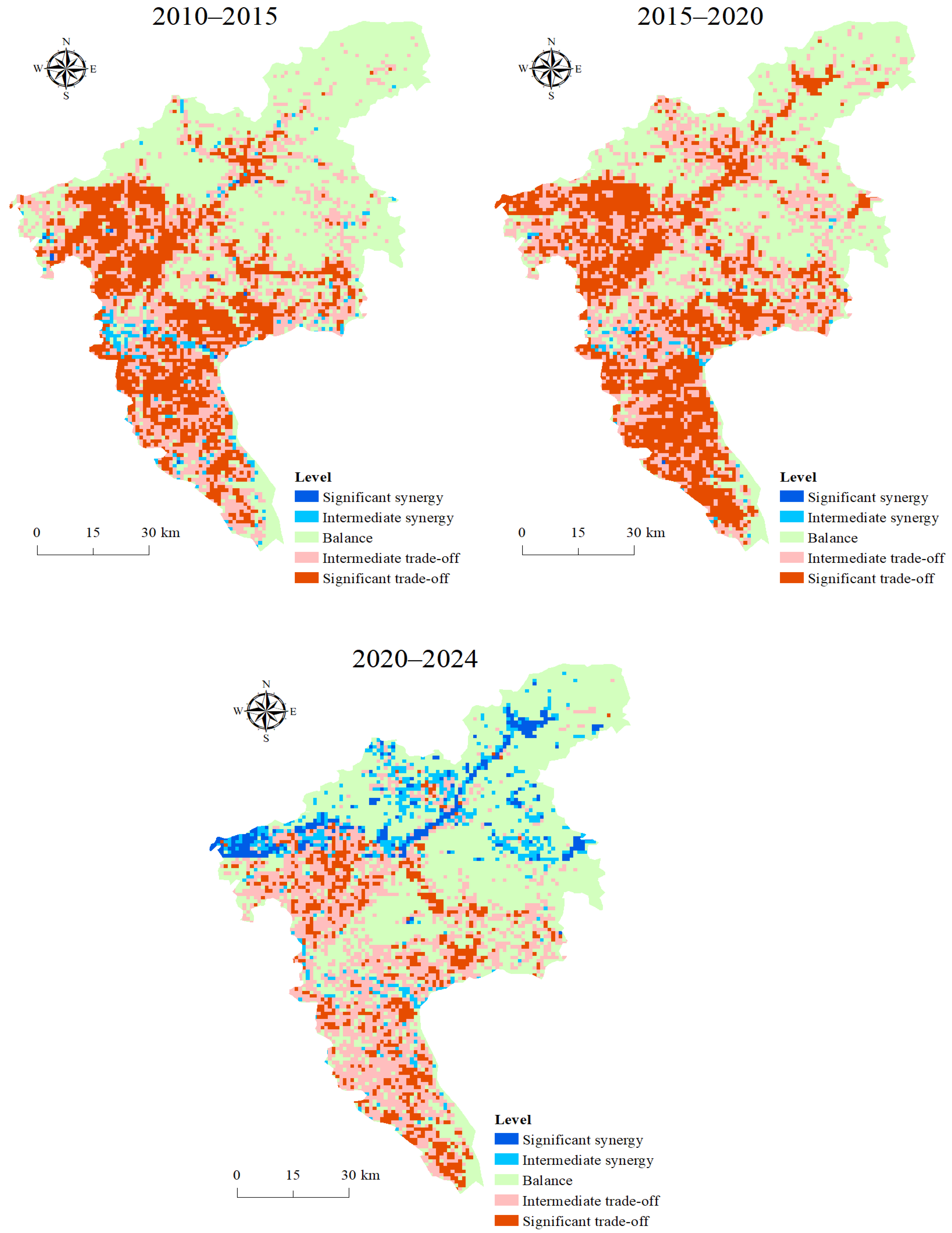
Based on the aforementioned method, the Trade-off/Synergy Index (TSI) for the three periods 2010–2015, 2015–2020 and 2020–2024 was calculated, and spatial mapping was conducted using the five-level classification standards (Figure 3). From an overall perspective, the balance and synergy among blue, green and grey spaces in Guangzhou exhibit distinct spatial differentiation—stable in the north and balanced in the central and southern regions. In terms of spatial distribution, areas with a high degree of balance are primarily concentrated in the central and southern regions, including Panyu, Nansha, the southern part of Baiyun, eastern Tianhe and Huangpu. These areas coincide with the regions experiencing the most intense urbanization in Guangzhou. The stable zones are primarily distributed in the mountainous areas of Conghua and Zengcheng in the north. In these areas, ecological conservation is the dominant function, urban development activities are relatively limited and changes in the structure of blue, green and grey spaces are minimal. Synergistic zones were virtually nonexistent in the early stages of the study but began to emerge significantly along the northern periphery in the later stages.

(1)

During the period of 2010–2015, the urban blue–green–grey space trade-off/synergy pattern in Guangzhou City was dominated by the trade-off type. The highly trade-off areas were distributed in a continuous and concentrated manner in the central and southern regions, with a wide coverage range and strong spatial continuity, mainly involving the northern part of Panyu District, Nansha District, the southern part of Baiyun District and the eastern part of Tianhe District, forming a nearly inverted triangle trade-off core area. The moderately trade-off areas were distributed around the highly trade-off areas, mainly distributed in the outer periphery of the trade-off core area and the junction of the central urban area and the northern mountainous area. The stable areas were mainly distributed in the mountainous and hilly areas of the northern Conghua District and Zengcheng District, showing a large-scale continuous pattern. However, during this period, the distribution of highly and moderately synergistic areas was extremely limited, almost indistinguishable in space, and appeared only sporadically at the local scale.

(2)

During 2015–2020, the balance/collaboration pattern continued the basic characteristics of the previous period, but the spatial range of the balance area further expanded. The most significant change was the substantial increase in the area of the moderate balance area, which spread from the central and southern regions to the north, beginning to invade originally relatively stable areas such as the western part of Zengcheng and the northern part of Huangpu. The distribution pattern of the high-balance area was generally consistent with the previous period, still concentrated in the central and southern regions, but the balance areas within were denser. The collaboration areas were still extremely rare, scattered only locally and high collaboration almost disappeared. This period was at the peak of Guangzhou’s Eastward and Southern Expansion strategy, with the focus of urban development gradually shifting to the east in Huangpu and Zengcheng, and to the south in Nansha. Urbanization development caused the originally stable urban fringe areas to become disturbed, with the balance relationship spreading from the core to the peripheral areas. At the same time, the continuous absence of collaboration areas indicated that the restorative growth of blue and green spaces during this period had not yet formed a scale.

(3)

The balance/synergy pattern of 2020–2024 has undergone significant changes. The most prominent feature is the significant increase in the area of synergy in the northern region: highly synergistic areas begin to appear patchily at the northern edge, mainly distributed in the northern part of Conghua District and the northeast of Zengcheng District, and extend in a strip-like manner along the waterway corridors such as the Liuxi River and Zeng River; the area of moderately synergistic regions has expanded significantly, forming a relatively continuous distribution area in the northern parts of Conghua, Zengcheng and Huangpu, and intertwining with the stable areas. Although the balance pattern in the central and southern regions still exists, it shows a trend of contraction. The spatial continuity of highly balanced areas has decreased, with some areas changing from highly balanced to moderately balanced or stable states. The distribution of moderately balanced areas has become more fragmented, no longer presenting a continuous strip-like pattern surrounding the highly balanced areas in the previous period, but instead showing a scattered distribution.

4.2. Spatiotemporal Evolution Characteristics of Waterlogging Disaster Risk in Guangzhou City

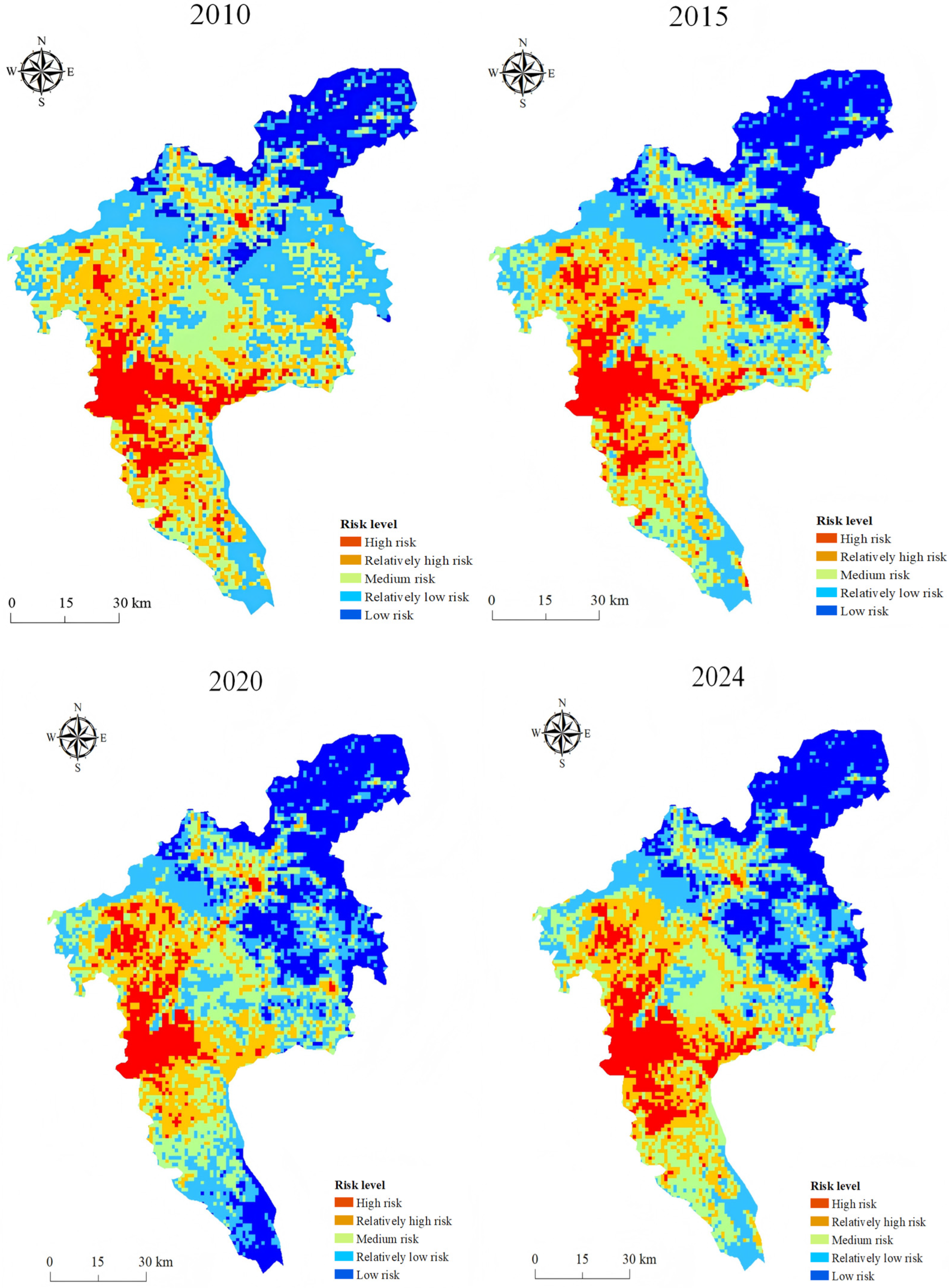
The risk of urban waterlogging in Guangzhou City shows a characteristic of being higher in the southwest and lower in the northeast (Figure 4). High-risk and relatively high-risk areas are mainly concentrated in the central urban areas of the southwest part of Guangzhou City, forming a high-risk agglomeration area centered on Yuexiu District and radiating to the surrounding areas. It covers most of the traditional central urban areas such as Yuexiu, Liwan, Haizhu and Tianhe, and extends to the southern part of Baiyun District and the northern part of Panyu District. In terms of spatial form, the high-risk areas show a strip-like distribution along both sides of the Pearl River. The low-risk and relatively low-risk areas are mainly distributed in the northern part of Conghua District and the northern part of Zengcheng District in the northeast of Guangzhou City, and the risk of urban waterlogging has remained at a relatively low level during the period from 2010 to 2024. The hilly area in the northern part of Huadu District also shows a relatively low risk level. The moderately risky areas are distributed in a ring between the high-risk and low-risk areas, forming a transitional zone between the two. This transitional zone is not uniformly distributed in space but undergoes dynamic changes as urban development advances.

4.3. Analysis of the Dynamic Response Process of Urban Blue–Green–Grey Space Trade-Off/Synergy to Waterlogging Disaster Risk

4.3.1. Analysis of the Correlation Between Urban Blue–Green–Grey Space Trade-Off/Synergy and the Risk of Waterlogging Disasters

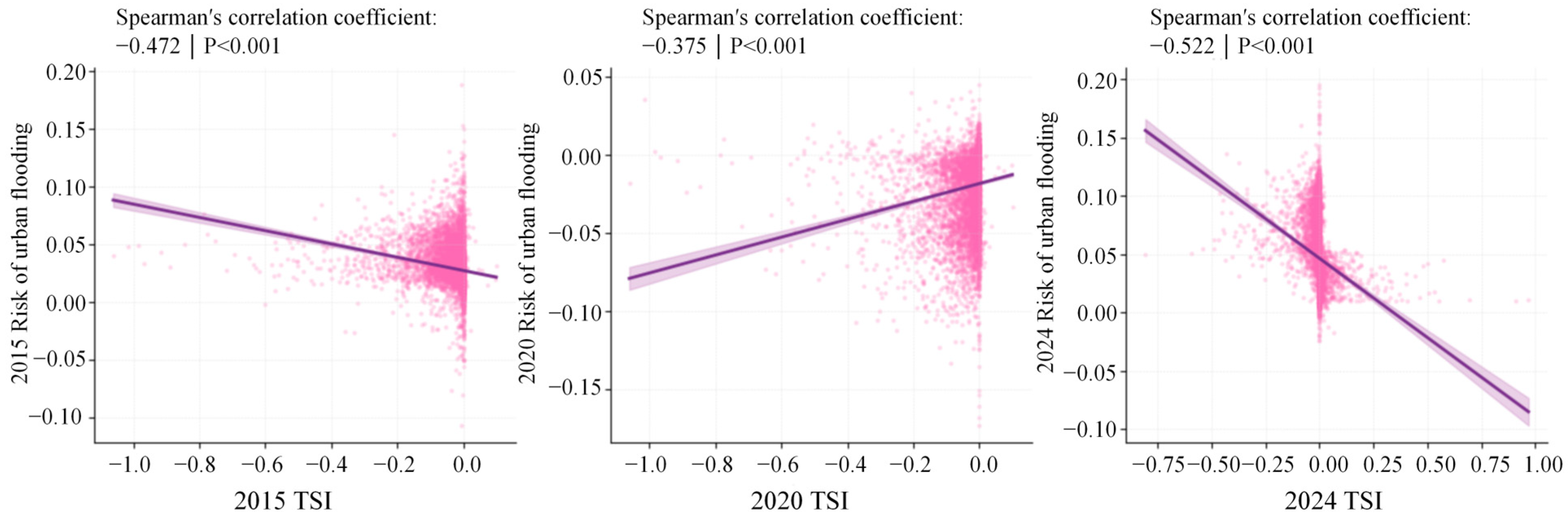
Figure 5 shows that the TSI across three periods is significantly correlated with the risk of waterlogging disasters, but the direction of correlation differs. In 2015, the TSI was significantly negatively correlated with risk change, and in 2024, it remained significantly negatively correlated. However, in 2020, it is significantly positively correlated.

The negative correlation in 2015 and 2024 indicates that the greater the decrease in TSI values (i.e., the more biased towards the trade-off state), the greater the increase in the risk of waterlogging disasters; the higher the TSI values (i.e., the more biased towards the synergy state), the smaller the increase in the risk of waterlogging disasters, or even a decrease. The phenomenon of positive correlation in 2020 is worth in-depth exploration. From the scatter plot distribution, most of the grid risk change values during this period are concentrated in the range from −0.15 to 0.05, with a slight bias towards negative values, indicating that the risk of waterlogging disasters in Guangzhou during 2015–2020 has been alleviated overall. In addition, the absolute value of the correlation coefficient in 2020 was significantly lower than in 2015 and 2024, indicating that the association between TSI and the change in waterlogging disaster risk during this period has weakened. This change may be related to the development of sponge cities, ecological restoration measures and adjustments to urban stormwater management strategies.

4.3.2. Analysis of the Difference in Urban Blue–Green–Grey Space Trade-Off/Synergy State Waterlogging Disaster Risk

(1)

Weighting/Synergistic Group Differences

As shown in

Table 3. Results of Kruskal–Wallis H test for risk changes under balance/synergy relationship in different periods.

Period	N	k	H	Data Frame	p	p_perm	ε2
2010–2015	7572	3	2251.343	2	<0.001	<0.001	0.297
2015–2020	7572	3	1387.922	2	<0.001	<0.001	0.183
2020–2024	7572	3	2815.333	2	<0.001	<0.001	0.372

Note: p is the approximate χ² p-value; p_perm is the p-value from 1000 permutation tests; ε² is the effect size.

, there are extremely significant differences in risk changes between the three types of synergy/balance/trade-off within the three periods (p values are all much less than 0.001), and the results of the permutation test also support this conclusion. From the perspective of effect size, the ε² values for the periods 2010–2015 and 2020–2024 are 0.297 and 0.372, respectively, indicating strong intergroup differentiation; the ε² value for the period 2015–2020 is 0.183, with relatively weak intergroup differences but still demonstrating clear practical differentiation. This indicates that at the grid scale, the trade-off/synergy state can form a stable differentiation of risk change levels.

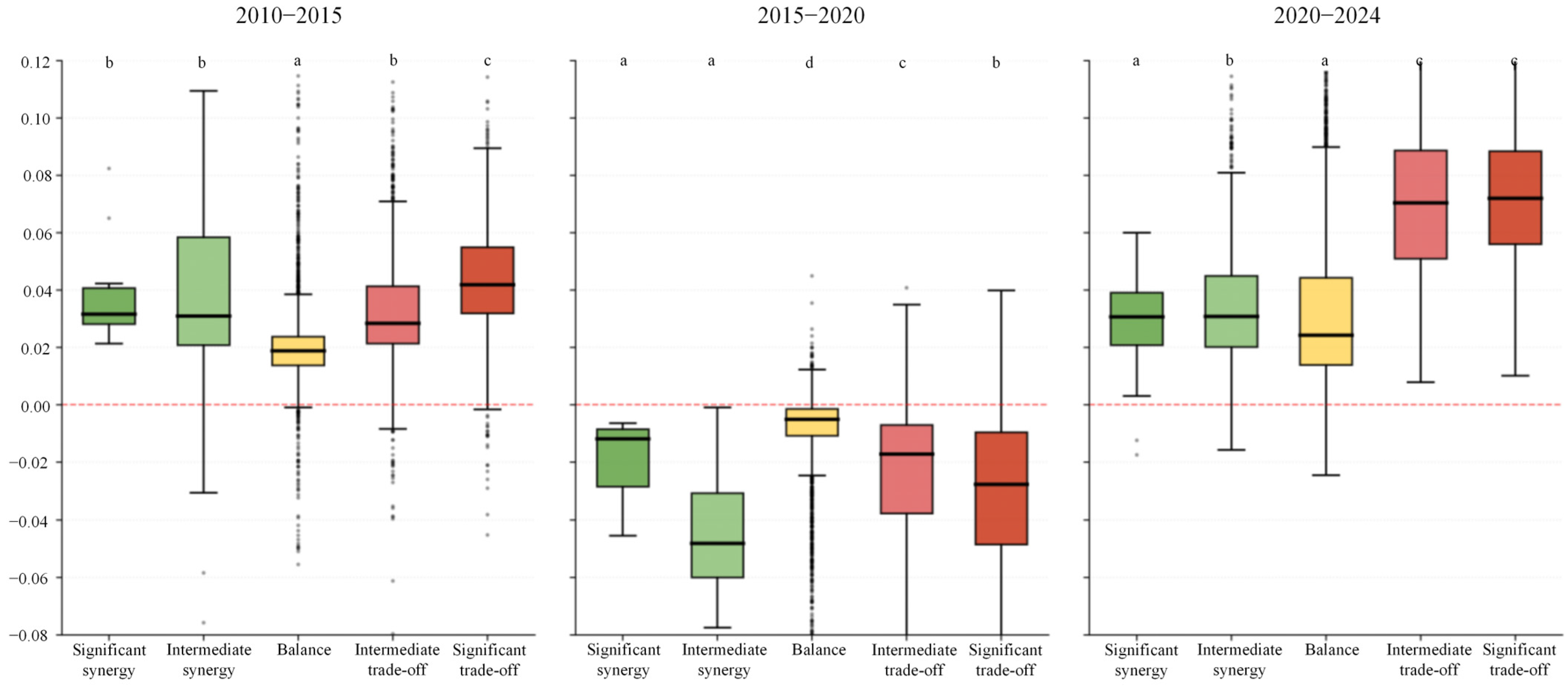
Combining

Table 4. Descriptive statistics of risk changes in each period under balance/synergy state.

Period	Type	n	Median [Q1, Q3]	Interquartile Range
2010–2015	Synergy	204	0.0312 [0.0214, 0.0573]	0.0360
2010–2015	Balance	3570	0.0188 [0.0138, 0.0237]	0.0099
2010–2015	Balance	3798	0.0352 [0.0249, 0.0496]	0.0248
2015–2020	Synergy	70	−0.0451 [−0.0594, −0.0285]	0.0309
2015–2020	Balance	2952	−0.0050 [−0.0107, −0.0014]	0.0093
2015–2020	Balance	4550	−0.0210 [−0.0446, −0.0079]	0.0366
2020–2024	Synergy	886	0.0308 [0.0203, 0.0418]	0.0216
2020–2024	Balance	3885	0.0243 [0.0138, 0.0443]	0.0304
2020–2024	Balance	2801	0.0708 [0.0521, 0.0885]	0.0364

Note: Q1 and Q3 are the 25th and 75th percentiles, respectively; IQR = Q3 − Q1.

and Figure 6, it can be seen that the risk changes in the three phases show a gradient type with consistent direction. The differences in risk changes between the synergistic group and the trade-off group exhibit significant period heterogeneity. From 2010 to 2015, the differences between the two groups were not significant (p = 0.272), with the median of the synergistic group (+0.0312) being close to that of the trade-off group (+0.0352), indicating that during this period, the impact of the synergy/trade-off state on risk changes was limited. From 2015 to 2020, the differences between the two groups reached an extremely significant level; the median reduction in risk for the synergistic group was −0.0451, and for the trade-off group was −0.0210, with the risk reduction of the synergistic group being 2.1 times that of the trade-off group, indicating that during the risk reduction period, the synergistic state could significantly amplify the reduction effect of risk. From 2020 to 2024, the differences between the two groups were also significant: the median increase in risk for the collaborative group was +0.0308, and for the trade-off group was +0.0708, with the risk increase of the synergistic group being only 43% of that of the trade-off group, indicating that during the risk increase period, the synergistic state could effectively suppress the increase in risk.

Post hoc comparison results (

Table 5. Dunn post hoc comparison (Holm correction).

Period	Comparison	Z	p_raw	p_holm	Significance
2010–2015	Synergy vs. Balance	13.274	<0.001	<0.001	***
2010–2015	Synergy vs. Trade-off	−1.991	0.046	0.046	**
2010–2015	Balance vs. Trade-off	−47.130	<0.001	<0.001	***
2015–2020	Synergy vs. Balance	−12.421	<0.001	<0.001	***
2015–2020	Synergy vs. Balance	−5.339	<0.001	<0.001	***
2015–2020	Balance vs. Trade-off	36.348	<0.001	<0.001	***
2020–2024	Synergy vs. Balance	2.837	0.005	0.005	**
2020–2024	Synergy vs. Balance	−30.489	<0.001	<0.001	***
2020–2024	Balance vs. Trade-off	−51.672	<0.001	<0.001	***

Note: Significance marking rules: ** (p_holm < 0.01), *** (p_holm < 0.001).

) further verify the above differences: except for the boundary between synergy and trade-off being significantly different during the period 2010–2015 (p_holm = 0.046), pairwise comparisons between the three categories reached ** and above significant levels for the other periods, indicating that the three-category results have good statistical stability and interpretability.

(2)

Analysis of differences between five-level classification groups

At the five-level classification, the overall differences in the three periods also reached an extremely significant level (Table 6), and the effect sizes for the 2010–2015 and 2020–2024 periods were 0.342 and 0.373, respectively, indicating that the differentiation between groups remains clear after refining the intensity. Compared to the three-level classification, the five-level classification can further reveal the phenomena of intensity gradient and boundary overlap:

First, the median of moderate synergy (0.0310) and moderate trade-off (0.0284) is relatively close (Table 7), and some pairwise comparisons are not significant, which statistically explains the marginal significance between the synergy group and the trade-off group in the three categories—when synergy/trade-off is merged, intragroup heterogeneity dilutes some differences. Second, the overall level of trade-off-related grades was in the high range from 2020 to 2024, and the difference between the two was not significant, suggesting that the risk increase during this period is more likely to manifest as entering the trade-off range, i.e., a significant increase.

During the 2010–2015 period, the results of Dunn’s post hoc comparisons, adjusted using Holm’s correction (Table 8), indicated significant differences among the various risk change categories. Specifically, highly synergistic versus balanced, moderately synergistic versus balanced, moderately synergistic versus highly trade-off, balanced versus moderately trade-off, balanced versus highly trade-off and moderately trade-off versus highly trade-off all reached the level of extreme significance (p < 0.001). In contrast, the differences between high synergy and moderate synergy, high synergy and moderate trade-off, high synergy and high trade-off, and moderate synergy and moderate trade-off were not significant (p > 0.05).

During the 2015–2020 period, highly significant differences were observed between “moderate synergy and balance,” “moderate synergy and moderate trade-off,” “moderate synergy and high trade-off,” “balance and moderate trade-off,” “balance and high trade-off” and “moderate trade-off and high trade-off” (p < 0.001). In contrast, no significant differences were observed between high synergy and moderate synergy, high synergy and balance, high synergy and moderate trade-off, or high synergy and high trade-off (p > 0.05), indicating that the risk variation characteristics of the high synergy type are relatively similar to those of the other categories.

During the 2020–2024 period, highly significant differences (p < 0.001) were observed between “high synergy and moderate trade-off,” “high synergy and high trade-off,” “moderate synergy and balance,” “moderate synergy and moderate trade-off,” “moderate synergy and high trade-off,” “balance and moderate trade-off” and “balance and high trade-off.” Furthermore, a significant difference was observed between “high synergy” and “moderate synergy” (p < 0.05), whereas the differences between “high synergy” and “balance,” as well as between “moderate trade-off” and “high trade-off,” were not significant (p > 0.05).

Overall, the differences among the five risk change types exhibit distinct similarities. Significant differences are primarily concentrated between the synergy and trade-off types, indicating that the synergy state in blue–green–grey spaces is strongly associated with the risk reduction process, while the trade-off state corresponds to higher levels of risk change. The differences between different synergy levels and between different trade-off levels are not significant, suggesting that the impact of varying degrees of spatial change within the same type on risk response is relatively similar; that is, the transition from a synergy to a trade-off state may be a key factor influencing risk change.

In general, 2010–2015 and 2020–2024 show an increase in risk, while 2015–2020 shows a decrease in risk; against this background, the trade-offs/synergies state and risk changes exhibit a repeatable correspondence: the increase in the risk increase option group is greater, and the decrease in the risk decrease option group is greater. In addition, the 2020–2024 period shows a stepwise increase in the balance interval, suggesting that, in certain spatial units, when the grey space expansion exceeds a threshold, or the drainage system capacity reaches its limit, the risk change will shift from slow to rapid increase.

Table 6. Results of Kruskal–Wallis H test for risk changes under five-level classification in different periods.

Period	N	k	H	Data Frame	p	p_perm	ε2
2010–2015	7572	5	2593.227	4	<0.001	<0.001	0.342
2015–2020	7572	5	1450.433	4	<0.001	<0.001	0.191
2020–2024	7572	5	2826.438	4	<0.001	<0.001	0.373

Note: The meaning of the statistics is the same as in Table 3.

Table 6. Results of Kruskal–Wallis H test for risk changes under five-level classification in different periods.

Period	N	k	H	Data Frame	p	p_perm	ε2
2010–2015	7572	5	2593.227	4	<0.001	<0.001	0.342
2015–2020	7572	5	1450.433	4	<0.001	<0.001	0.191
2020–2024	7572	5	2826.438	4	<0.001	<0.001	0.373

Note: The meaning of the statistics is the same as in Table 3.

Table 7. Descriptive statistics of risk changes under five-level classification in different periods.

Period	Type	n	Median [Q1, Q3]	Interquartile Range
2010–2015	Significant synergy	13	0.0317 [0.0282, 0.0406]	0.0124
2010–2015	Intermediate synergy	191	0.0310 [0.0208, 0.0584]	0.0376
2010–2015	Balance	3570	0.0188 [0.0138, 0.0237]	0.0099
2010–2015	Intermediate trade-off	1940	0.0284 [0.0214, 0.0413]	0.0199
2010–2015	Significant trade-off	1858	0.0419 [0.0319, 0.0549]	0.0230
2015–2020	Significant synergy	6	−0.0119 [−0.0285, −0.0085]	0.0200
2015–2020	Intermediate synergy	64	−0.0482 [−0.0601, −0.0307]	0.0293
2015–2020	Balance	2952	−0.0050 [−0.0107, −0.0014]	0.0093
2015–2020	Intermediate trade-off	2289	−0.0171 [−0.0378, −0.0070]	0.0308
2015–2020	Significant trade-off	2261	−0.0276 [−0.0485, −0.0095]	0.0390
2020–2024	Significant synergy	324	0.0307 [0.0208, 0.0390]	0.0182
2020–2024	Intermediate synergy	562	0.0309 [0.0202, 0.0450]	0.0248
2020–2024	Balance	3885	0.0243 [0.0138, 0.0443]	0.0304
2020–2024	Intermediate trade-off	2026	0.0704 [0.0510, 0.0886]	0.0377
2020–2024	Significant trade-off	775	0.0720 [0.0560, 0.0884]	0.0324

Note: The statistical criteria are the same as in Table 4; attention should be paid to the fact that the sample sizes of some extreme categories are relatively small (e.g., significant synergy n = 13 for the period 2010–2015, significant synergy n = 6 for the period 2015–2020).

Table 7. Descriptive statistics of risk changes under five-level classification in different periods.

Period	Type	n	Median [Q1, Q3]	Interquartile Range
2010–2015	Significant synergy	13	0.0317 [0.0282, 0.0406]	0.0124
2010–2015	Intermediate synergy	191	0.0310 [0.0208, 0.0584]	0.0376
2010–2015	Balance	3570	0.0188 [0.0138, 0.0237]	0.0099
2010–2015	Intermediate trade-off	1940	0.0284 [0.0214, 0.0413]	0.0199
2010–2015	Significant trade-off	1858	0.0419 [0.0319, 0.0549]	0.0230
2015–2020	Significant synergy	6	−0.0119 [−0.0285, −0.0085]	0.0200
2015–2020	Intermediate synergy	64	−0.0482 [−0.0601, −0.0307]	0.0293
2015–2020	Balance	2952	−0.0050 [−0.0107, −0.0014]	0.0093
2015–2020	Intermediate trade-off	2289	−0.0171 [−0.0378, −0.0070]	0.0308
2015–2020	Significant trade-off	2261	−0.0276 [−0.0485, −0.0095]	0.0390
2020–2024	Significant synergy	324	0.0307 [0.0208, 0.0390]	0.0182
2020–2024	Intermediate synergy	562	0.0309 [0.0202, 0.0450]	0.0248
2020–2024	Balance	3885	0.0243 [0.0138, 0.0443]	0.0304
2020–2024	Intermediate trade-off	2026	0.0704 [0.0510, 0.0886]	0.0377
2020–2024	Significant trade-off	775	0.0720 [0.0560, 0.0884]	0.0324

Note: The statistical criteria are the same as in Table 4; attention should be paid to the fact that the sample sizes of some extreme categories are relatively small (e.g., significant synergy n = 13 for the period 2010–2015, significant synergy n = 6 for the period 2015–2020).

Table 8. Post hoc Dunn comparisons under five-level classification (Holm correction).

Period	Comparison	Z	p_raw	p_holm	Significance
2010–2015	Significant synergy vs. Intermediate synergy	0.585	0.559	0.808	ns
2010–2015	Significant synergy vs. Balanced	4.004	<0.001	<0.001	***
2010–2015	Significant synergy vs. Intermediate trade-off	1.104	0.269	0.808	ns
2010–2015	Significant synergy vs. Significant trade-off	−1.051	0.293	0.808	ns
2010–2015	Intermediate synergy vs. Balance	12.723	<0.001	<0.001	***
2010–2015	Intermediate synergy vs. Intermediate trade-off	1.842	0.065	0.262	ns
2010–2015	Intermediate synergy vs. Significant trade-off	−6.056	<0.001	<0.001	***
2010–2015	Balance vs. Intermediate trade-off	28.547	<0.001	<0.001	***
2010–2015	Balance vs. Significant trade-off	49.118	<0.001	<0.001	***
2010–2015	Intermediate trade-off vs. Significant trade-off	18.481	<0.001	<0.001	***
2015–2020	Significant synergy vs. Intermediate synergy	1.971	0.049	0.195	ns
2015–2020	Significant synergy vs. Balance	−1.793	0.073	0.219	ns
2015–2020	Significant synergy vs. Intermediate trade-off	0.033	0.974	1.000	ns
2015–2020	Significant synergy vs. Significant trade-off	0.588	0.556	1.000	ns
2015–2020	Intermediate synergy vs. Balance	12.459	<0.001	<0.001	***
2015–2020	Intermediate synergy vs. Intermediate trade-off	−6.533	<0.001	<0.001	***
2015–2020	Intermediate synergy vs. Significant trade-off	−4.741	<0.001	<0.001	***
2015–2020	Balance vs. Intermediate trade-off	26.794	<0.001	<0.001	***
2015–2020	Balance vs. Significant trade-off	34.824	<0.001	<0.001	***
2015–2020	Intermediate trade-off vs. Significant trade-off	7.657	<0.001	<0.001	***
2020–2024	Significant synergy vs. Intermediate synergy	−2.821	0.005	0.014	*
2020–2024	Significant synergy vs. Balance	−0.332	0.740	0.740	ns
2020–2024	Significant synergy vs. Intermediate trade-off	21.381	<0.001	<0.001	***
2020–2024	Significant synergy vs. Significant trade-off	20.470	<0.001	<0.001	***
2020–2024	Intermediate synergy vs. Balance	3.935	<0.001	<0.001	***
2020–2024	Intermediate synergy vs. Intermediate trade-off	22.706	<0.001	<0.001	***
2020–2024	Intermediate synergy vs. Significant trade-off	20.891	<0.001	<0.001	***
2020–2024	Balance vs. Intermediate trade-off	45.982	<0.001	<0.001	***
2020–2024	Balance vs. Significant trade-off	33.935	<0.001	<0.001	***
2020–2024	Intermediate trade-off vs. Significant trade-off	−1.774	0.076	0.152	ns

Note: Significance marking rules: ns (p_holm ≥ 0.05), * (p_holm < 0.05), *** (p_holm < 0.001).

Table 8. Post hoc Dunn comparisons under five-level classification (Holm correction).

Period	Comparison	Z	p_raw	p_holm	Significance
2010–2015	Significant synergy vs. Intermediate synergy	0.585	0.559	0.808	ns
2010–2015	Significant synergy vs. Balanced	4.004	<0.001	<0.001	***
2010–2015	Significant synergy vs. Intermediate trade-off	1.104	0.269	0.808	ns
2010–2015	Significant synergy vs. Significant trade-off	−1.051	0.293	0.808	ns
2010–2015	Intermediate synergy vs. Balance	12.723	<0.001	<0.001	***
2010–2015	Intermediate synergy vs. Intermediate trade-off	1.842	0.065	0.262	ns
2010–2015	Intermediate synergy vs. Significant trade-off	−6.056	<0.001	<0.001	***
2010–2015	Balance vs. Intermediate trade-off	28.547	<0.001	<0.001	***
2010–2015	Balance vs. Significant trade-off	49.118	<0.001	<0.001	***
2010–2015	Intermediate trade-off vs. Significant trade-off	18.481	<0.001	<0.001	***
2015–2020	Significant synergy vs. Intermediate synergy	1.971	0.049	0.195	ns
2015–2020	Significant synergy vs. Balance	−1.793	0.073	0.219	ns
2015–2020	Significant synergy vs. Intermediate trade-off	0.033	0.974	1.000	ns
2015–2020	Significant synergy vs. Significant trade-off	0.588	0.556	1.000	ns
2015–2020	Intermediate synergy vs. Balance	12.459	<0.001	<0.001	***
2015–2020	Intermediate synergy vs. Intermediate trade-off	−6.533	<0.001	<0.001	***
2015–2020	Intermediate synergy vs. Significant trade-off	−4.741	<0.001	<0.001	***
2015–2020	Balance vs. Intermediate trade-off	26.794	<0.001	<0.001	***
2015–2020	Balance vs. Significant trade-off	34.824	<0.001	<0.001	***
2015–2020	Intermediate trade-off vs. Significant trade-off	7.657	<0.001	<0.001	***
2020–2024	Significant synergy vs. Intermediate synergy	−2.821	0.005	0.014	*
2020–2024	Significant synergy vs. Balance	−0.332	0.740	0.740	ns
2020–2024	Significant synergy vs. Intermediate trade-off	21.381	<0.001	<0.001	***
2020–2024	Significant synergy vs. Significant trade-off	20.470	<0.001	<0.001	***
2020–2024	Intermediate synergy vs. Balance	3.935	<0.001	<0.001	***
2020–2024	Intermediate synergy vs. Intermediate trade-off	22.706	<0.001	<0.001	***
2020–2024	Intermediate synergy vs. Significant trade-off	20.891	<0.001	<0.001	***
2020–2024	Balance vs. Intermediate trade-off	45.982	<0.001	<0.001	***
2020–2024	Balance vs. Significant trade-off	33.935	<0.001	<0.001	***
2020–2024	Intermediate trade-off vs. Significant trade-off	−1.774	0.076	0.152	ns

Note: Significance marking rules: ns (p_holm ≥ 0.05), * (p_holm < 0.05), *** (p_holm < 0.001).

4.4. Analysis of the Contribution of Urban Blue, Green and Grey Space Changes to the Risk Change in Urban Waterlogging Disasters

4.4.1. Results of Spatial Econometric Model Selection

Table 9. Global Moran’s I test results for waterlogging disaster risk.

Period	Moran’s I	z Value	p-Value	Spatial Pattern
2015	0.7950	85.98	<0.001 ***	Significant aggregation
2020	0.8341	141.18	<0.001 ***	Highly concentrated
2024	0.9122	154.40	<0.001 ***	Extremely concentrated

Note: *** indicates p < 0.001. The spatial weight matrix is constructed based on the Queen adjacency criterion.

shows the global Moran’s I test results for the risk of waterlogging disasters across three periods. The results indicate that Moran’s I for the three periods are all significant positive values (p < 0.001), indicating that the risk of waterlogging disasters presents a significant positive spatial autocorrelation feature, and there is an increasing evolution trend from period to period. The spatial differentiation between high-risk and low-risk areas becomes increasingly evident, and the spatial dependence of risk continues to strengthen.

Table 10. Lagrange multiplier test results and model selection.

Inspection Item	2015	2020	2024
LM-Lag	5507.54 ***	17649.73 ***	21359.67 ***
LM-Error	4907.23 ***	16821.68 ***	20484.28 ***
Robust LM-Lag	602.46 ***	873.28 ***	998.62 ***
Robust LM-Error	42.15 ***	45.22 ***	123.23 ***

Note: *** indicates p < 0.001. Model selection is based on Anselin’s (1988) decision tree [73].

and

Table 11. Comparison of fitting effects of four types of spatial econometric models.

Period	Model	Log-Likelihood	AIC	BIC	R2/Quasi-R2
2015	Ordinary Least Squares	19508.45	−39008.89	−38981.16	0.0932
	SAR	21,066.88	−42123.76	−42,089.10	0.7765
	SEM	21,001.73	−41995.46	−41967.73	0.1105
	SDM	21099.41	−42182.82	−42127.36	0.7745
2020	Ordinary Least Squares	17823.66	−35639.33	−35611.60	0.0736
	SAR	23480.24	−46950.48	−46915.82	0.8340
	SEM	23486.38	−46964.77	−46937.04	0.0416
	SDM	23,520.70	−47025.41	−46969.95	0.8334
2024	Ordinary Least Squares	15961.29	−31914.58	−31886.85	0.0861
	SAR	24000.31	−47990.62	−47955.96	0.9154
	SEM	23996.21	−47984.43	−47956.70	0.0085
	SDM	24065.69	−48115.37	−48059.91	0.9151

Note: The smaller the AIC and BIC, the better, and the larger the log-likelihood and R-squared, the better.

show the results of the Lagrange multiplier test and the model-fitting effects for each period. In 2015, 2020 and 2024, both robust LM tests were significant, indicating the presence of spatial lag and spatial spillover effects. At the same time, the explanatory power of the spatial effect models (SAR, SEM, SDM) was significantly greater than that of OLS, and the SDM model should be chosen.

4.4.2. Analysis of the Impact of Urban Blue, Green and Grey Space Changes on the Risk of Waterlogging Disasters

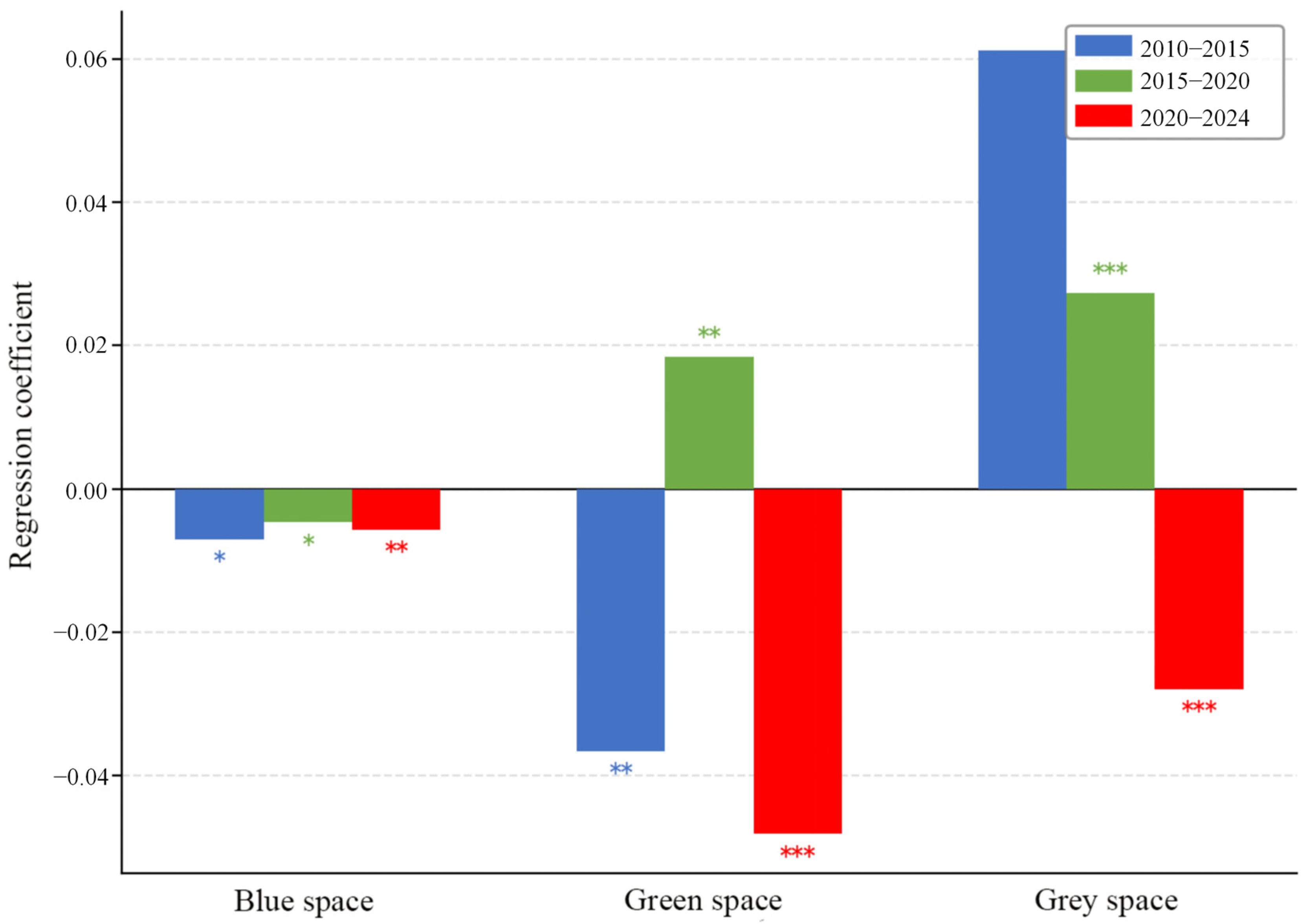
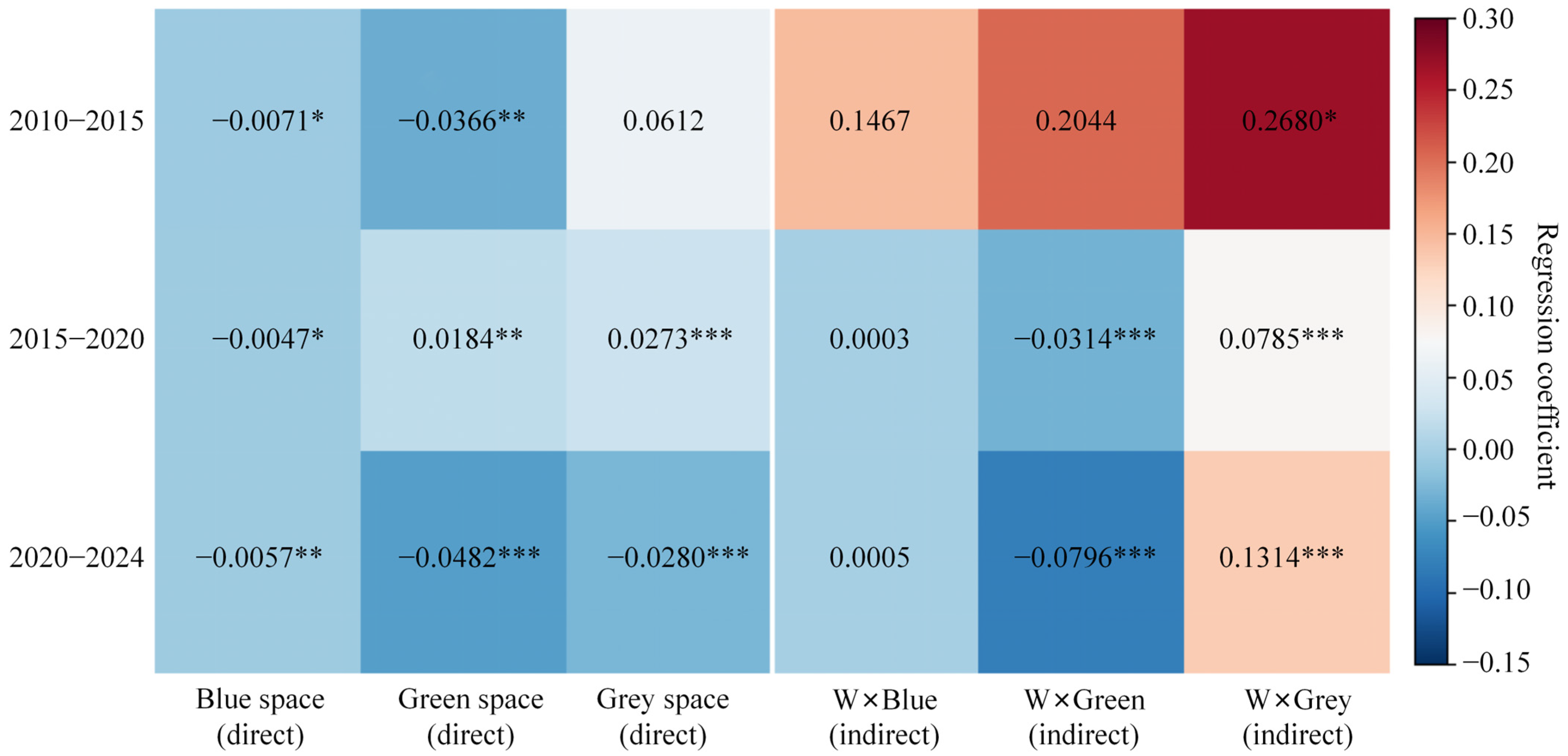
(1) Direct effects of urban blue, green and grey spaces (Figure 7,

Table 12. Spatial Durbin Model (SDM) results.

Variable	2010–2015	2015–2020	2020–2024
Spatial Autoregressive Coefficient ρ	0.7950 ***	0.9072 ***	0.9218 ***
Constant Term	0.0078 ***	−0.0016 ***	0.0035 ***
Direct Effect
Blue Space Ratio Change	−0.0071 *	−0.0047 *	−0.0057 **
Green Space Ratio Change	−0.0366 **	0.0184 **	−0.0482 ***
Grey Space Ratio Change	0.0612	0.0273 ***	−0.0280 ***
Indirect Effects (Spillover Effects)
W × Blue Space	0.1467	0.0003	0.0005
W × Green Space	0.2044	−0.0314 ***	−0.0796 ***
W × Grey Space	0.2680 *	0.0785 ***	0.1314 ***

Note: *** indicates p < 0.001, ** indicates p < 0.01, * indicates p < 0.05; W is the spatial weight matrix.

); the direct effects of blue spaces were significantly negative across all three time periods, with coefficients of −0.0071, −0.0047 and −0.0057, respectively. This indicates that for every 1 percentage point increase in the proportion of local blue spaces, the risk of local urban flooding decreases by approximately 0.005 to 0.007. The stability of this negative effect confirms the stormwater retention and flood control functions of water bodies: blue spaces such as rivers, lakes, wetlands and fish ponds can temporarily store runoff during heavy rainfall, reduce flood peaks and delay the time to first return, thereby effectively reducing the probability and intensity of urban flooding. The absolute values of the coefficients across the three time periods remained within the range of 0.0047 to 0.0071, with a fluctuation range of only 0.0024. This indicates that the storage capacity of core water bodies—such as the main stem of the Pearl River and large reservoirs—remained relatively stable during the study period. Conversely, the shrinkage of blue spaces under the trade-off scenario signifies a systemic loss of storage capacity. These encroached-upon rivers, fish ponds and wetlands originally served as decentralized stormwater retention and detention features; their disappearance directly weakens the region’s ability to reduce flood peaks.

The direct effects of green spaces have fluctuated over different periods. Both the 2010–2015 and 2020–2024 periods showed significant negative effects, reflecting the disaster-mitigation functions of vegetation in retaining rainfall, enhancing infiltration and slowing surface runoff. However, during 2015–2020, the direct effect of green spaces turned positive. In conjunction with the rapid urbanization and land-use conversion processes during this period, the creation and preservation of green spaces tended to occur in low-lying areas with poor drainage and inherently higher risk. At the same time, considering the overall change in risk, the risk variation observed during 2015–2020 may be related to the combination of below-average rainfall during that period and the phased implementation of “sponge city” initiatives and drainage and flood prevention projects. Consequently, the statistical analysis shows a positive correlation between the increase in the proportion of green space and changes in risk, rather than green space itself having the effect of exacerbating risk. From 2020 to 2024, as the rate of urbanization slowed significantly and the delineation of ecological red lines and the implementation of national spatial planning took effect, the structure of existing green spaces stabilized, spatial selection bias gradually dissipated and the intrinsic disaster-mitigation function of green spaces reemerged statistically. The absolute value of the direct effect coefficient during this period was the highest among the three time periods, representing a 31.69% increase compared to the first period. This indicates that sponge city construction, urban stormwater management and ecological restoration measures have achieved certain results, and that the quality and quantity of green space are also continuously improving.

The direct effect of changes in the proportion of grey space shifted from positive to negative. The coefficient was positive but not significant (0.0612) from 2010 to 2015; it was significantly positive (0.0273) from 2015 to 2020; and it turned into a significantly negative value of −0.0280 from 2020 to 2024. This indicates that the expansion of construction land increases impervious areas, hinders stormwater infiltration and exacerbates surface waterlogging. In 2016, Guangzhou was selected as a national pilot city for sponge city construction. Since then, the city has systematically promoted low-impact development measures citywide, including permeable paving, sunken green spaces, rain gardens and grass swales. These measures have ensured that newly added grey space is no longer entirely impervious in the traditional sense but possesses a certain capacity for stormwater infiltration and retention. At the same time, efforts to enhance the “sponge city” capabilities of existing built-up areas during urban renewal have also improved the runoff characteristics of existing grey spaces. The shift from a positive to a negative direct effect of grey spaces between 2020 and 2024 provides a technical pathway for achieving a synergistic state—through planning controls and engineering measures, the traditional correlation between the expansion of grey spaces and increased risks of urban flooding can be mitigated.

(2) The spillover effects of urban blue–green–grey spaces. The indirect effects (spillover effects) reflect the cross-regional transmission of changes in neighboring urban blue–green–grey spaces on local waterlogging disaster risks, revealing the spatial externality characteristics of waterlogging disaster risks. If the direct effects explain how the trade-off state intensifies risks at the local scale, then the indirect effects reveal how the trade-off state leads to the regional spread of risks through spatial spillover.

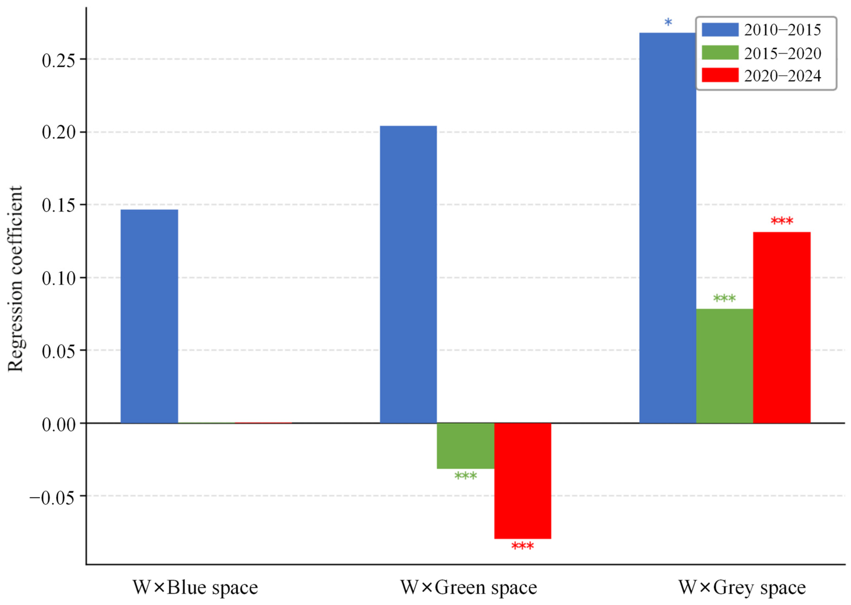
The indirect effects of blue space did not reach significance in all three periods (Figure 8). Further explanation indicates that the mitigating function of the water body mainly acts at the local scale, with limited spatial spillover effects to the neighborhood. The blue space in Guangzhou is structured around the Pearl River system, distributed in a branching network pattern, and the hydrological connectivity between water bodies mainly extends along the longitudinal direction of the river channels. The regulating function of the blue space mainly serves its own catchment area, with limited impact on grids that are spatially adjacent but hydrologically not directly connected. The role of blue space in balancing/collaboration mainly manifests at the local scale, and its protection and restoration should focus on the point or linear layout of key areas rather than on a uniform distribution over a large area.

The indirect effects of green spaces have evolved from insignificant to significantly negative. The coefficient was 0.2044 but not significant from 2010 to 2015, turned to −0.0314 from 2015 to 2020, and further enhanced to −0.0796 from 2020 to 2024. The negative spillover effect means that an increase in the proportion of green spaces in the neighborhood can reduce the risk of local waterlogging disasters, reflecting the regional collaborative value of green spaces in reducing disaster risk. In the early stages of the study, the distribution of green spaces was relatively even but fragmented, forming an interlaced mosaic pattern with grey spaces and poor connectivity between green patches, making it difficult to form systematic runoff interception and transmission barrier functions; thus, the spillover effect was not significant. With urbanization advancing, green spaces in the central and southern regions were largely occupied, and the remaining green spaces gradually concentrated in the northern mountainous areas, forming a continuous ecological barrier, with Pingshan and Zengcheng in the north as the core. This passive agglomeration phenomenon enhanced the spatial continuity and system integrity of green spaces. The absolute value of the indirect effect of green spaces from 2020 to 2024 has exceeded its direct effect, with a ratio of 1.65:1. Therefore, in the process of promoting the transformation of urban blue, green and grey spaces from trade-offs to synergy, the planning and layout of green spaces should not only focus on the improvement in green rates of individual plots but should also pay attention to the systematic construction of green space networks. By connecting scattered patches into a network through ecological corridors, green belts and other linear elements, the regional collaborative disaster reduction effect can be fully utilized.

The indirect effects of the grey space are all significantly positive in the three periods, with coefficients of 0.2680 (p < 0.05), 0.0785 (p < 0.001) and 0.1314 (p < 0.001). The positive spillover effect indicates that an increase in the proportion of grey space in the neighborhood will exacerbate the risk of local waterlogging disasters, revealing the spatial externality characteristics of urban waterlogging. Its transmission mechanism includes two paths: surface runoff, that is, excess runoff generated from impermeable areas upstream or around flows, and downstream flow along the terrain slope. When it exceeds the carrying capacity of the downstream drainage system, it causes waterlogging in low-lying areas; the other is drainage network transmission, that is, the urban drainage network connects each area into an integrated whole. Excessive runoff from upstream high-flow areas is transmitted downstream through the network. When the network is full, or backflow occurs, poor drainage occurs in the downstream area. The concentrated, contiguous distribution of the grey space not only exacerbates local risks but also produces negative spillover effects on surrounding areas through runoff transmission, leading to the regional spread of risks as the weighing area expands.

The temporal evolution of the indirect effects of the grey space shows a “high-low-rising” trend, which contains rich policy information. The indirect effect was highest from 2010 to 2015 (0.2680), which was related to the rapid expansion of the grey space during this period, but the relatively lagging construction of drainage infrastructure, with the runoff inter-regional transfer effect being more prominent. From 2015 to 2020, the indirect effect decreased to 0.0785, a 70.71% decline, which was attributed to the large-scale renovation of drainage networks and the construction of regulating facilities during this period. Although the trade-off area experienced severe greyification during this period, the construction of drainage and waterlogging prevention infrastructure, implemented to some extent simultaneously, partially interrupted the regional runoff transmission path, offsetting the negative spillover effects of the expansion of the grey space. This is also one of the important reasons why the TSI and risk changes showed an abnormal positive correlation during this period.

However, from 2020 to 2024, the indirect effects of the grey area once again increased to 0.1314, a 67.39% increase from the previous period. This rebound phenomenon is worth alerting to, and may be related to two factors: first, the large amount of impervious surface accumulated in the past continues to produce excessive runoff, and its regional conduction effect gradually becomes apparent with time lag, making it difficult for existing drainage facilities to completely digest the runoff input across regions; second, the frequent occurrence of extreme rainfall events has amplified the negative spillover effects of the grey area; under the scenario of excessive rainfall, the intercepting capacity of the drainage system is greatly reduced, and the runoff conduction effect is re-emphasized. More importantly, the direct effect of the grey area from 2020 to 2024 has changed from positive to negative (−0.0280), while the indirect effect has increased from 0.1314, indicating a clear trend of differentiation. This differentiation has important policy implications: the construction of sponge city construction, urban stormwater management and ecological restoration measures can effectively improve the local runoff characteristics in the grey area, but its inhibitory effect on runoff conduction across regions is limited.

The analysis results of the direct and indirect effects (Figure 9) can systematically explain the mechanism of the trade-off/synergistic impact on the risk of waterlogging disasters. The shrinkage of the blue space weakens the regional regulation and storage capacity, with the direct effect coefficient stable in the range from −0.0047 to −0.0071; the shrinkage of the green space weakens the interception and infiltration function and destroys the connectivity of the green network, with the direct effect coefficient ranging from −0.0366 to −0.0482 and the indirect effect coefficient from −0.0314 to −0.0796, the combined impact is more significant; the expansion of the grey space not only increases the local runoff but more importantly, through cross-regional spillover, it amplifies the risk transmission. The three work together to form “increased runoff—reduced regulation and storage—intensified spillover,” which is the intrinsic reason for the continuous deterioration of waterlogging disaster risk due to the trade-off state.

The mechanism for improving the risk of collaborative states lies in functional complementarity.” The data from 2020 to 2024 provide an outline of the collaborative state: the blue space maintains stable regulating functions, the indirect effects of the green space have exceeded the direct effects, and the regional collaborative effects have significantly increased. However, the recovery of the indirect effects of the grey space warns us that the realization of collaborative states cannot rely solely on single-point transformation but also requires overall planning and control of the grey space layout at the basin scale to block cross-regional risk transmission paths.

5. Conclusions and Discussion

5.1. Conclusions

(1)

Evolution of Blue–Green–Grey Spaces and Their Trade-off/Synergy Characteristics

Between 2010 and 2024, the blue–green–grey spatial pattern in Guangzhou underwent significant changes, generally characterized by a trade-off between the reduction of blue and green spaces and the expansion of grey spaces. However, with the advancement of measures such as ecological restoration, urban renewal and sponge city construction, the degree of trade-off among blue, green and grey spaces has diminished in recent years, and some areas have gradually shifted from a state of trade-off to one of synergy. The research findings indicate that, against the backdrop of rapid urbanization, the urban spatial pattern does not involve continuous, unidirectional expansion but rather involves constant adjustments between development and ecological conservation; however, significant spatial heterogeneity still exists across different regions.

(2)

Spatial Response Characteristics of the Relationship Between Blue–Green–Grey Spaces and Flood Risk

The trade-off/synergy relationship among blue, green and grey spaces exhibits significant spatial correlations with urban flood risk. Overall, areas with increased trade-offs among blue, green and grey spaces tend to correspond to higher predicted flood risks, whereas areas with synergistic configurations exhibit lower flood risk levels. At the same time, this influence exhibits a certain degree of spatial spillover effect, indicating that urban flood risk is affected not only by changes in local spatial patterns but also by the combined effects of spatial configurations in surrounding areas. Therefore, the optimization of blue, green and grey spaces requires transcending administrative boundaries and focusing on synergistic planning at the regional scale.

(3)

Practical Implications

The findings of this study offer a new perspective on urban flood risk management and spatial optimization. Urban flood control planning should not rely solely on the expansion of traditional grey infrastructure but should comprehensively consider the protection and restoration of blue and green ecological spaces. By optimizing the allocation of blue–green–grey spaces, urban stormwater regulation capacity and ecological resilience can be enhanced. Given the differences in trade-off and synergy states across various regions, zoned and categorized management strategies can be adopted to achieve a dynamic balance between urban development and ecological security.

(4)

Future Research Directions

Future research could further integrate multiscale spatial analysis, hydrodynamic modeling and causal inference methods to thoroughly elucidate the mechanisms through which different configurations of blue–green–grey spaces influence flood risk. Additionally, by incorporating future climate change scenarios and urban development simulations, researchers can assess long-term trends in urban flood risk under various spatial optimization strategies.

5.2. Discussion

This study developed a Trade-off/Synergy Assessment Framework (TSI) for blue–green–grey spaces. This study examined the relationship between the allocation of blue, green and grey spaces and urban flood risk from the perspectives of spatial associations and variable contributions. Existing research generally agrees that blue–green infrastructure can reduce urban flood risk by enhancing stormwater retention capacity, while the expansion of impervious surfaces resulting from rapid urbanization increases flood risk. However, existing studies have largely focused on the independent effects of individual spatial elements, with insufficient attention paid to the dynamic trade-offs and synergies among blue, green and grey spaces. This study further reveals the relationship between the synergistic/trade-off changes of multiple types of urban spatial elements and flood risk responses, the areas where the balance between blue, green and grey spaces becomes more pronounced typically correspond to higher flood risks, while the areas with coordinated configurations show lower risk levels, possibly related to their comprehensive regulation of the rainfall runoff process. Green spaces can delay the transformation of rainfall into surface runoff through processes such as vegetation interception, soil infiltration and increased surface roughness, while blue spaces like rivers and lakes have functions of temporarily storing and regulating rainwater. When blue and green spaces form a good spatial coordination, their ecological regulation function may shift from the local effect of a single patch to a continuous rainwater regulation process, that is, through “interception—infiltration—transmission—retention” and other links, it can reduce the speed of surface runoff formation and reduce the accumulation of runoff in a short period of time. In contrast, the expansion of grey spaces and the increase in flood risk may mainly be related to the urban surface impermeability and the reduction of natural regulation spaces. When the continuous expansion of construction land and other impermeable surfaces occurs, rainfall infiltration is inhibited, more rainfall quickly accumulates in the form of surface runoff and may increase the peak value of short-term runoff, thereby further increasing the flood risk. This indicates that shifting from a single land use type to the spatial configuration relationship among blue, green and grey infrastructure can help better understand the formation mechanism of urban flood risks. The TSI method can comprehensively characterize the relative relationships among blue, green and grey spaces and identify states of trade-offs and synergies during urban spatial evolution. Compared to evaluation methods based on single land use indicators, it is better suited for analyzing complex spatial transformations in the context of rapid urbanization. At the same time, this framework is highly scalable and can be integrated with spatial statistical models and machine learning methods to explore the relationship between urban spatial configuration and ecological risks. However, as the TSI is primarily constructed based on spatial area and landscape pattern characteristics, it has not yet fully accounted for differences in spatial quality and ecological functions, such as green space types, vegetation structure and water body storage and regulation capacity. Therefore, future research could further integrate ecological function indicators, hydrological process models and machine learning models to improve the characterization of the actual regulatory capacity of blue–green–grey spaces.

Although this study uses Guangzhou as a case study, the TSI framework has certain generalizability for regions experiencing rapid urbanization and high flood risk, and is particularly applicable to high-density coastal cities and cities with dense river networks. However, given differences among cities in terms of climatic conditions, topographic characteristics and stages of urban development, adjustments must still be made in practical applications to account for regional hydrological environments and planning needs.

This study still involves some uncertainties. Firstly, due to limitations in data structure and research conditions, this paper has not conducted a systematic VIF correlation test on the variables of SDM. Therefore, it is impossible to completely rule out the potential multiple collinearity issues among the variables. Although the variable selection was mainly based on theoretical mechanisms and existing studies, there may be a certain degree of information overlap among some indicators, which may affect the stability of parameter estimation. Therefore, the conclusions regarding the direction of influence of each explanatory variable and the spatial spillover effect in this paper should be understood as results in a statistical correlation sense. The specific mechanism of their effects still needs to be verified through further variable selection and robustness tests. Secondly, the spatial Durbin model uses the Queen adjacency matrix to construct spatial weighting relationships; while this method can reflect spatial proximity effects, it struggles to fully characterize river network connectivity and hydrological propagation processes, which may affect the identification of certain spatial spillover effects. This study gives limited consideration to socioeconomic factors (such as population density, economic level and drainage network conditions) as well as spatial scale effects, which may lead to a certain degree of uncertainty. Future research could incorporate hydrological connectivity weights, multiscale sensitivity analyses and more comprehensive socioeconomic and infrastructure data to further validate the mechanisms through which the optimization of blue–green–grey spaces mitigates urban flood risk.

References

1. Huang, H.; Wang, X.; Liu, L. A review on urban pluvial floods: Characteristics, mechanisms, data, and research methods. Prog. Geogr. 2021, 40, 1048–1059. [Google Scholar] [CrossRef] [Scilit]
2. Cheng, X.; Li, C. The evolution trend, key features and countermeasures of urban flood risk. China Flood Drought Manag. 2015, 25, 6–9. [Google Scholar]
3. Li, W.; Ding, X.; Wang, Z. Research progress of urban waterlogging depth estimation methods. J. Spatio-Temporal Inf. 2026, 33, 04012. [Google Scholar]
4. Zhu, J.; Zhou, W.; Yu, W.; Wang, W. Block-level spatial integration of population density, social vulnerability, and heavy precipitation reveals intensified urban flooding risk. Sustain. Cities Soc. 2024, 117, 105984. [Google Scholar] [CrossRef] [Scilit]
5. Kleinert, S.; Horton, R. Urban design: An important future force for health and wellbeing. Lancet 2016, 388, 2848–2850. [Google Scholar] [CrossRef] [Scilit] [PubMed]
6. Qin, X.; Wu, Y.; Huang, H.; Yang, X.; Gao, L. Impact of impervious surface spatial morphologies on urban waterlogging: Insights from a cascade modeling chain at catchment scale. Sustain. Cities Soc. 2025, 134, 106912. [Google Scholar] [CrossRef] [Scilit]
7. Rentschler, J.; Avner, P.; Marconcini, M.; Su, R.; Strano, E.; Vousdoukas, M.; Hallegatte, S. Global evidence of rapid urban growth in flood zones since 1985. Nature 2023, 622, 87–92. [Google Scholar] [CrossRef] [Scilit] [PubMed]
8. Tullos, D. How to achieve better flood-risk governance in the United States. Proc. Natl. Acad. Sci. USA 2018, 115, 3731–3734. [Google Scholar] [CrossRef] [Scilit] [PubMed]
9. Zhang, X.; Kang, A.; Song, Q.; Guo, Y.; Liu, Y.; Lei, X.; Wang, H. Characteristics and risk management of urban surface flooding in Guangzhou, China: Insights from 2022 ground monitoring. J. Hydrol. Reg. Stud. 2024, 53, 101831. [Google Scholar] [CrossRef] [Scilit]
10. Shin, S.; Kim, J.; Park, D.; Kang, T.; Jung, K. Assessment of Flood Damage Costs for Different Storm Surge, Climate Change, and Drainage Scenarios in Busan, South Korea. JAWRA J. Am. Water Resour. Assoc. 2025, 61, e70052. [Google Scholar] [CrossRef] [Scilit]
11. Wang, Y.; Zhang, Q.; Zhang, J.; Lin, K. Impact of 2D and 3D factors on urban flooding: Spatial characteristics and interpretable analysis of drivers. Water Res. 2025, 280, 123537. [Google Scholar] [CrossRef] [Scilit] [PubMed]
12. Li, Y.; Hu, X.; Zhang, K.; Chen, J.; Hu, X. Flood response strategies for megacities in the context of global extreme rainstorms patterns—Taking Beijing as an example. China Water Resour. 2023, 12, 31–36. [Google Scholar] [CrossRef]
13. Jiang, Y.; Zevenbergen, C.; Ma, Y. Urban pluvial flooding and stormwater management: A contemporary review of China’s challenges and “sponge cities” strategy. Environ. Sci. Policy 2018, 80, 132–143. [Google Scholar] [CrossRef] [Scilit]
14. Rosenberger, L.; Leandro, J.; Pauleit, S.; Erlwein, S. Sustainable stormwater management under the impact of climate change and urban densification. J. Hydrol. 2021, 596, 126137. [Google Scholar] [CrossRef] [Scilit]
15. Li, C.; Cheng, X.; Shen, R.; Liu, Q. New Characteristics and Formation Mechanism of Flood and Waterlogging Disasters in the Context of Rapid Urbanization. J. Catastrophol. 2019, 34, 57–62. [Google Scholar]
16. Li, X.; Zhao, M.; Lin, F. Exploration of the integration of “Blue-Green-Grey” sponge space for drainage and flood management in Shanghai. China Flood Drought Manag. 2023, 33, 14–18. [Google Scholar]
17. Grimm, N.B.; Faeth, S.H.; Golubiewski, N.E.; Redman, C.L.; Wu, J.; Bai, X.; Briggs, J.M. Global Change and the Ecology of Cities. Science 2008, 319, 756–760. [Google Scholar] [CrossRef] [Scilit] [PubMed]
18. Huang, G.; Yang, G.; Zeng, B.; Lv, Y. Urban flood disaster control based on green-grey-blue infrastructure integration. J. Zhengzhou Univ. (Eng. Sci.) 2023, 44, 14–22. [Google Scholar]
19. Liu, J.; Mei, C.; Shao, W.; Wang, J. Flood Risk Management Transmission from Spatial Master Planning to Regulatory Planning: Practice and Exploration in Guangzhou. J. Hydraul. Eng. 2022, 53, 789–797. [Google Scholar]
20. McDougall, C.W.; Hanley, N.; Quilliam, R.S.; Oliver, D.M. Blue space exposure, health and well-being: Does freshwater type matter? Landsc. Urban Plan. 2022, 224, 104446. [Google Scholar] [CrossRef] [Scilit]
21. White, M.P.; Elliott, L.R.; Gascon, M.; Roberts, B.; Fleming, L.E. Blue space, health and well-being: A narrative overview and synthesis of potential benefits. Environ. Res. 2020, 191, 110169. [Google Scholar] [CrossRef] [Scilit] [PubMed]
22. Hunter, R.F.; Cleland, C.; Cleary, A.; Droomers, M.; Wheeler, B.W.; Sinnett, D.; Nieuwenhuijsen, M.J.; Braubach, M. Environmental, health, wellbeing, social and equity effects of urban green space interventions: A meta-narrative evidence synthesis. Environ. Int. 2019, 130, 104923. [Google Scholar] [CrossRef] [Scilit] [PubMed]
23. Li, J.; Trivic, Z. Impact of “blue-green diet” on human health and wellbeing: A systematic review of potential determinants in shaping the effectiveness of blue-green infrastructure (BGI) in urban settings. Sci. Total Environ. 2024, 926, 171397. [Google Scholar] [CrossRef] [Scilit] [PubMed]
24. Venkataramanan, V.; Packman, A.I.; Peters, D.R.; Lopez, D.; McCuskey, D.J.; McDonald, R.I.; Miller, W.M.; Young, S.L. A systematic review of the human health and social well-being outcomes of green infrastructure for stormwater and flood management. J. Environ. Manag. 2019, 246, 868–880. [Google Scholar] [CrossRef] [Scilit] [PubMed]
25. Chen, M.; Papadikis, K.; Jun, C. An investigation on the non-stationarity of flood frequency across the UK. J. Hydrol. 2021, 597, 126309. [Google Scholar] [CrossRef] [Scilit]
26. Dong, X.; Guo, H.; Zeng, S. Enhancing future resilience in urban drainage system: Green versus grey infrastructure. Water Res. 2017, 124, 280–289. [Google Scholar] [CrossRef] [Scilit] [PubMed]
27. Tansar, H.; Duan, H.-F.; Mark, O. A multi-objective decision-making framework for implementing green-grey infrastructures to enhance urban drainage system resilience. J. Hydrol. 2023, 620, 129381. [Google Scholar] [CrossRef] [Scilit]
28. Xu, C.; Rahman, M.; Haase, D.; Wu, Y.; Su, M.; Pauleit, S. Surface runoff in urban areas: The role of residential cover and urban growth form. J. Clean. Prod. 2020, 262, 121421. [Google Scholar] [CrossRef] [Scilit]
29. Miller, J.D.; Kim, H.; Kjeldsen, T.R.; Packman, J.; Grebby, S.; Dearden, R. Assessing the Impact of Urbanization on Storm Runoff in a Peri-Urban Catchment Using Historical Change in Impervious Cover. J. Hydrol. 2014, 515, 59–70. [Google Scholar] [CrossRef] [Scilit]
30. Kim, H.; Lee, D.-K.; Sung, S. Effect of Urban Green Spaces and Flooded Area Type on Flooding Probability. Sustain. Water Qual. Ecol. 2016, 8, 134. [Google Scholar] [CrossRef] [Scilit]
31. Jia, R.; Fu, C.; Gan, Y. Integrated green-grey-blue system: A bibliometric analysis-based review. In Proceedings of the Fifth International Conference on Green Energy, Environment, and Sustainable Development (GEESD 2024), Mianyang, China, 28–30 June 2024. [Google Scholar]
32. Al-Humaiqani, M.M.; Al-Ghamdi, S.G. Integrating green–blue–grey infrastructure for sustainable urban flood risk management: Enhancing resilience and advantages. In Sustainable Cities in a Changing Climate: Enhancing Urban Resilience; John Wiley and Sons: Hoboken, NJ, USA, 2023; pp. 207–226. [Google Scholar] [CrossRef] [Scilit]
33. Bakhshipour, A.E.; Dittmer, U.; Haghighi, A.; Nowak, W. Hybrid green-blue-grey decentralized urban drainage systems design, a simulation-optimization framework. J. Environ. Manag. 2019, 249, 109364. [Google Scholar] [CrossRef] [Scilit] [PubMed]
34. Yin, D.; Zhang, X.; Cheng, Y.; Jia, H.; Jia, Q.; Yang, Y. Can flood resilience of green-grey-blue system cope with future uncertainty? Water Res. 2023, 242, 120315. [Google Scholar] [CrossRef] [Scilit] [PubMed]
35. He, M.; Yuan, C.; Zhang, X.; Wang, P.; Yao, C. Impacts of green-blue-grey infrastructures on high-density urban thermal environment at multiple spatial scales: A case study in Wuhan. Urban Clim. 2023, 52, 101714. [Google Scholar] [CrossRef] [Scilit]
36. Gunawardena, K.R.; Wells, M.J.; Kershaw, T. Utilising green and bluespace to mitigate urban heat island intensity. Sci. Total Environ. 2017, 584, 1040–1055. [Google Scholar] [CrossRef] [Scilit] [PubMed]
37. Volk, M. Modelling ecosystem services: Current approaches, challenges and perspectives. Sustain. Water Qual. Ecol. 2015, 5, 1–2. [Google Scholar] [CrossRef] [Scilit]
38. Kumar, P.; Debele, S.E.; Khalili, S.; Halios, C.H.; Sahani, J.; Aghamohammadi, N.; Andrade, M.d.F.; Athanassiadou, M.; Bhui, K.; Calvillo, N.; et al. Urban heat mitigation by green and blue infrastructure: Drivers, effectiveness, and future needs. Innovation 2024, 5, 100588. [Google Scholar] [CrossRef] [Scilit] [PubMed]
39. Fan, J.; Liu, B.; Lei, T.; Sun, Y.; Ma, Y.; Guo, R.; Chen, D.; Zhou, K.; Li, S.; Gao, X. Exploring how economic level drives urban flood risk. Nat. Commun. 2025, 16, 4857. [Google Scholar] [CrossRef] [Scilit] [PubMed]
40. Zhu, L.; Gao, C.; Wu, M.; Zhu, R. Integrating blue–green infrastructure with grey infrastructure for climate-resilient surface water flood management in the plain river networks. Land 2025, 14, 634. [Google Scholar] [CrossRef] [Scilit]
41. Yuanita, C.N.; Sagala, S. Blue-green infrastructure in Jakarta’s fringe: An analysis of accessibility to blue-green spaces as a flood solution in Bekasi City. Int. J. Disaster Risk Reduct. 2025, 121, 105425. [Google Scholar] [CrossRef] [Scilit]
42. Thorsson, S.; Bäcklin, O.; Friberg, J.; Eriksson, S.F.; Haghighatafshar, S.; Konarska, J.; Kotze, S.; Lindberg, F.; Malmberg, C.-A.; Rayner, D.; et al. A framework for integrated assessment of blue-green infrastructure: A decision support tool for evaluating climate adaptation and social benefits in relation to construction and maintenance costs. Cities 2025, 166, 106239. [Google Scholar] [CrossRef] [Scilit]
43. Orak, N.H.; Smail, L. A Bayesian Network model to integrate blue-green and grey infrastructure systems for different urban conditions. J. Environ. Manag. 2025, 375, 124293. [Google Scholar] [CrossRef] [Scilit] [PubMed]
44. Gomes, M.V.R.; Battemarco, B.P.; Guimarães, L.F.; de Oliveira, A.K.B.; Rutigliani, V.d.A.; Cabral, F.M.; Bezerra, R.d.O.P.; Lourenço, I.B.; Rezende, O.M.; de Magalhães, P.C.; et al. The use of blue-green infrastructure as a multifunctional approach to watersheds with socio-environmental vulnerability. Blue-Green Syst. 2021, 3, 281–297. [Google Scholar] [CrossRef] [Scilit]
45. Azis, S.S.A.; Zulkifli, N.A.A. Green roof for sustainable urban flash flood control via cost benefit approach for local authority. Urban For. Urban Green. 2021, 57, 126876. [Google Scholar] [CrossRef] [Scilit]
46. Chen, X.; Wang, X. Blue–Green Infrastructure Network Planning in Urban Small Watersheds Based on Water Balance. Land 2025, 14, 1652. [Google Scholar] [CrossRef] [Scilit]
47. Hysa, A. Introducing Transversal Connectivity Index (TCI) as a method to evaluate the effectiveness of the blue-green infrastructure at metropolitan scale. Ecol. Indic. 2021, 124, 107432. [Google Scholar] [CrossRef] [Scilit]
48. Alves, A.; Vojinovic, Z.; Kapelan, Z.; Sanchez, A.; Gersonius, B. Exploring trade-offs among the multiple benefits of green-blue-grey infrastructure for urban flood mitigation. Sci. Total Environ. 2020, 703, 134980. [Google Scholar] [CrossRef] [Scilit] [PubMed]
49. Sun, C.; Rao, Q.; Wang, M.; Liu, Y.; Xiong, Z.; Zhao, J.; Fan, C.; Rana, M.A.I.; Li, J.; Zhang, M. Multi-stage optimization of drainage systems for integrated grey–green infrastructure under backward planning. Water 2024, 16, 1825. [Google Scholar] [CrossRef] [Scilit]
50. Chen, W.; Wang, X.; Deng, S.; Liu, C.; Xie, H.; Zhu, Y. Integrated urban flood vulnerability assessment using local spatial dependence-based probabilistic approach. J. Hydrol. 2019, 575, 454–469. [Google Scholar] [CrossRef] [Scilit]
51. Zhu, X.; Xu, Z.; Liu, C.; Sun, Z.; Weng, W.; Li, Y. From constraints to compatibility: Evolution, key issues, and solutions in integration green and grey infrastructure planning. Chin. J. Appl. Ecol. 2025, 36, 2874–2884. [Google Scholar]
52. Li, S.S.; Leitao, J.P.; Bach, P.M. A drainage network-based impact matrix to support targeted blue-green-grey stormwater management solutions. Sci. Total Environ. 2024, 912, 168623. [Google Scholar] [CrossRef] [Scilit] [PubMed]
53. Zhang, C.; Wang, J.; Liu, J.; Lv, Y.; Chen, J.; Yang, Z.; Zhang, N. Performance assessment for the integrated green-grey-blue infrastructure under extreme rainfall scenarios. Front. Ecol. Evol. 2023, 11, 1242492. [Google Scholar] [CrossRef] [Scilit]
54. Liu, Z. Unraveling the efficiency-equity trade-off in urban heat island mitigation by blue–green–grey space optimization in China. Urban Clim. 2026, 68, 103041. [Google Scholar] [CrossRef] [Scilit]
55. Tian, J.; Zhao, L.; Xia, J. Mechanisms of Urban Spatial Patterns and Infrastructure on Urban Flooding: Research Progress. Trop. Geogr. 2026, 46, 419–433. [Google Scholar]
56. Wang, Y.; Peng, L.; Yang, L.E.; Wang, Z.; Deng, X. Attributing effects of classified infrastructure management on mitigating urban flood risks: A case study in Beijing, China. Sustain. Cities Soc. 2024, 101, 105141. [Google Scholar] [CrossRef] [Scilit]
57. Liu, Y.; Zhang, X.; Liu, J.; Gong, L.; Gui, H. Assessment of Flood Control Effectiveness of Green-Grey-Blue Infrastructure During Extreme Rainstorms: A Case Study of East-sha Lake Watershed. J. Basic Sci. Eng. 2024, 32, 740–753. [Google Scholar]
58. Chen, X.; Fang, Z.; Liu, J.; Chai, Y.; Yu, H.; Zhou, H.; Gao, Y. Mitigation effects of integrated green-grey-blue-control systems on urban flooding in plain regions. Water Resour. Manag. 2025, 39, 5313–5338. [Google Scholar] [CrossRef] [Scilit]
59. Zhang, H.; Hong, Q.; Jiang, Y.; Xie, Y. The synergistic effects of green-blue-grey infrastructure for flood risk management in plain river network areas. J. Environ. Manag. 2025, 392, 126671. [Google Scholar] [CrossRef] [Scilit] [PubMed]
60. Cheng, Y.; Hou, Q.; Xie, M. Urban Green Space Planning Method Based on Low Impact Development: Research on Planning Mechanism under Digital Landscape Technology. Digit. Landsc. 2019, 35, 5–12. [Google Scholar]
61. Zhou, K.; Wei, X.; Wang, Y.; Wang, J.; Wang, Z.; Zhang, Y. Spatiotemporal evolution and prediction of blue–green–grey-space carbon stocks in Henan Province, China. Front. Environ. Sci. 2025, 13, 1545455. [Google Scholar] [CrossRef] [Scilit]
62. Guo, Y.; Lu, X.; Wang, Y. Responses of birds with different habitat preferences to urban blue-green spaces: A systematic review and meta-analysis at a global scale. Biol. Conserv. 2025, 307, 111190. [Google Scholar] [CrossRef] [Scilit]
63. Qu, Z.; Zhang, Q.; Zhang, R. The optimization of urban blue-green spatial layout based on dual performances: A case study on Putuo District in Shanghai. J. Nanjing For. Univ. 2023, 47, 235–243. [Google Scholar]
64. Potter, J.D.; Brooks, C.; Donovan, G.; Cunningham, C.; Douwes, J. A perspective on green, blue, and grey spaces, biodiversity, microbiota, and human health. Sci. Total Environ. 2023, 892, 164772. [Google Scholar] [CrossRef] [Scilit] [PubMed]
65. Sun, M.; Liu, J.; Li, X.; Li, P.; Xiao, Z. Urban-rural difference and scale effect of ecosystem services of blue-green infrastructure. Chin. J. Appl. Ecol. 2024, 35, 3295–3303. [Google Scholar] [CrossRef] [Scilit] [PubMed]
66. Wu, R.; Sun, H.; Yan, D. Evaluation of flood disaster risk in China-Pakistan Economic Corridor by combination weighting based on improved game theory and grid data. Trans. Chin. Soc. Agric. Eng. 2021, 37, 145–154. [Google Scholar]
67. Kong, X.; Sun, Y. Risk Assessment of Flood Disaster in Harbin City Based on GIS. Water Conserv. Sci. Technol. Econ. 2024, 30, 95–100. [Google Scholar]
68. Liu, J.; Zhang, B.; Zhu, Y.; Zhang, Z. Investigation into the coupling of urban flood resilience and ecosystem services in the Songhua River Basin, Jilin Province. J. Saf. Environ. 2024, 24, 4870–4880. [Google Scholar]
69. Deng, X.; Li, Z.; Gibson, J. A review on trade-off analysis of ecosystem services for sustainable land-use management. J. Geogr. Sci. 2016, 26, 953–968. [Google Scholar] [CrossRef] [Scilit]
70. Wang, X.; Zhou, L.; López-Carr, D.; Song, Y.; Gao, H.; Che, T.; Liu, Z.; Wei, W. Urban grey-green scales: A new perspective for assessing dynamic spatial trade-offs. Int. J. Appl. Earth Obs. Geoinf. 2025, 142, 104708. [Google Scholar] [CrossRef] [Scilit]
71. He, B.; Tong, Y.; Gao, Y.; Zhou, M.; Li, P.; Zhang, Y. Comprehensive Evaluation of the Implementation Effect of Standardization of Oil Type Gas Prevention and Management Based on AHP-Entropy Weight Method. J. Green Sci. Technol. 2025, 27, 156–162. [Google Scholar] [CrossRef]
72. Liu, Y.; Wang, S.; Wang, X.; Jiang, D.; Ravindranath, N.H.; Rahman, A.; Htwe, N.M.; Vijitpan, T. Flood risk assessment in Bangladesh, India and Myanmar based on the AHP weight method and entropy weight method. Geogr. Res. 2020, 39, 1892–1906. [Google Scholar] [CrossRef]
73. Anselin, L. Model validation in spatial econometrics: A review and evaluation of alternative approaches. Int. Reg. Sci. Rev. 1988, 11, 279–316. [Google Scholar] [CrossRef] [Scilit]
Figure 1. Overview of the study area. Data source: Administrative divisions data of Guangzhou City (2024), Chinese basic geographic information data, Land cover data of Wuhan University (CLCD), compiled and calculated by the first author.
Land 15 01529 g001
Figure 2. Overall framework of the study. Construction and drawing of this study.
Land 15 01529 g002
Figure 3. Spatial and temporal distribution of the Trade-off/Synergy Index from 2010 to 2024. Data source: land use data (2010–2024), compiled and calculated by the first author.
Land 15 01529 g003
Figure 4. Spatial distribution of waterlogging disaster risk in four periods from 2010 to 2024. Data source: meteorological station data and related statistical data, which have been collated and calculated by the first author.
Land 15 01529 g004
Figure 5. Correlation between blue–green–grey trade-off/synergy and waterlogging disaster risk changes from 2020 to 2024. Data source: land use data and flood disaster risk data, calculated and drawn by the first author.
Land 15 01529 g005
Figure 6. Boxplot of risk changes over different periods under synergy/trade-off relationships. Data source: blue–green–grey spatial Trade-off/Synergy Index and Flooding Disaster Risk Index from 2010 to 2024 (2010–2024), calculated, statistically analyzed and plotted by the first author in stages. Note: The box is Q1–Q3, the horizontal line inside the box is the median; the whiskers are 1.5 × IQR; outliers are represented by small, semi-transparent points; the red dashed line is the 0 baseline; within the same period, shared letters indicate non-significant differences (Dunn–Holm, p ≥ 0.05). The y-axis range is set uniformly at the 1–99% quartiles of the full sample, with a fixed step of 0.02.
Land 15 01529 g006
Figure 7. Direct effect of the proportion change in urban blue–green–grey spaces on the risk change in waterlogging disasters. Data source: blue–green–grey space data and flood disaster risk data (2010–2024), compiled and plotted by the first author based on the spatial Durbin model. Note: *** indicates p < 0.001, ** indicates p < 0.01, * indicates p < 0.05.
Land 15 01529 g007
Figure 8. Temporal changes in direct and indirect effects of three types of spaces. Data source: blue–green–grey space data and flood disaster risk data (2010–2024), compiled by the first author, and estimated and plotted based on the spatial Durbin model. Note: *** indicates p < 0.001, * indicates p < 0.05.
Land 15 01529 g008
Figure 9. Temporal changes in the direct and indirect effects of urban blue, green and grey spaces from 2000 to 2024. Data source: urban blue, green and grey space data and flood disaster risk data (2000–2024), compiled by the first author, and estimated and plotted annually based on the spatial Durbin model. Note: *** indicates p < 0.001, ** indicates p < 0.01, * indicates p < 0.05.
Land 15 01529 g009