H-FANet: A Hierarchical Multi-Scale Attention Network for Hyperspectral-LiDAR Land Cover Classification

Abstract

Accurate land cover classification is critical for geographic information science. However, the fusion of hyperspectral and LiDAR data remains constrained by insufficient spectral-geometric coupling and limited scale representation. To address these challenges, we propose H-FANet, a hierarchical fusion attention network with a three-branch backbone (spectral, spatial, and elevation). Multi-scale enhancement modules are embedded in the spatial and elevation branches to capture scale-invariant features through hierarchical aggregation with convolutional splitting. For cross-modal interaction, H-FANet adopts a two-level fusion strategy: shape-level shallow cross-attention for geometric alignment and spectral-level deep residual fusion for semantic integration. Experiments on three benchmark datasets showed that H-FANet achieved overall accuracies of 99.13 ± 0.06% on Trento, 97.43 ± 0.06% on Houston 2013, and 92.11 ± 0.05% on the Muufl Gulfport datasets. The network outperformed five comparison methods by approximately 1.7–2.2% in overall accuracy. Ablation studies confirm the contributions of the multi-scale enhancement and hierarchical fusion modules. This GeoAI-driven framework improved land cover identification accuracy and could be applied to fields such as environmental monitoring, urban land use analysis, and ecological protection.

1. Introduction

With the continuous progress of remote sensing technology and sensor platforms, multi-source remote sensing data has become crucial in related fields such as environmental monitoring, resource investigation, and urban planning [1]. Hyperspectral images (HSIs), light detection and ranging (LiDAR), and other similar data sources provide complementary information from the perspectives of spectrum and spatial structure, significantly boosting the accuracy and reliability of target classification [2]. However, differences in resolution, noise levels, and information representation methods among multi-source data bring significant challenges to the fusion process [3]. How to effectively utilize the rich spectral information in hyperspectral data along with the elevation and structural advantages of LiDAR, and maintain and correlate their complementary characteristics during the fusion process, remains one of the core difficulties in current remote sensing applications [4].

In recent years, deep learning (DL) methods have received extensive attention in the field of remote sensing image analysis. Convolutional neural networks (CNNs) have demonstrated powerful performance in tasks such as remote sensing image classification, object detection, and semantic segmentation. Their achievement is attributed to their utilization of large, labeled datasets and their hierarchical feature abstraction capabilities [5,6]. In addition, Ullah et al. [7] conducted a comprehensive review of deep learning-based hyperspectral image feature learning, pointing out that although model performance is constantly improving, how to extract highly discriminative features under limited labeled samples is still the key research direction.

With the advancement of research, fusion strategies for heterogeneous and multi-source data are also constantly evolving. Cascade fusion can be classified into pixel-level, feature-level, and decision-level methods based on the stage at which fusion occurs in the network [8,9,10,11]. However, traditional cascaded methods have limited capabilities in integrating diverse attributes, especially when dealing with heterogeneous data. Under such circumstances, multi-scale feature learning has become a key focus of attention for both the academic and industrial communities. Multi-scale learning enables the model to simultaneously consider fine-grained local textures and global macroscopic structures, thus enhancing its adaptability and discriminative ability when processing targets of different sizes and shapes [12]. Lu Di et al. [13] introduced the multi-scale feature aggregation module (MSFA) and the multi-scale feature distribution module (MSFD), and adopted a pyramid-structured fusion strategy to hierarchically integrate features from the lower to the higher levels, enriching the context information and ensuring that the feature maps at each level can retain the original semantic and cross-layer semantic features.

Simultaneously, the “Attention Mechanism” has shown promising results in remote sensing data analysis by explicitly learning the importance of different dimensions or regions [14]. In existing work, the SIAM model [15] incorporates a parameter-free spatial cross-attention module that generates channel-wise and spatial-wise attention maps from two directions and combines them into a 3D attention map, enabling the inference of spatially intersecting important regions and capturing location-aware information. Wu et al. [16] proposed a spectral-spatial extensive kernel attention network for HSI classification, utilizing two consecutive spectral-spatial attention blocks with large convolution kernels to jointly capture and enhance features across spectral and spatial domains. Integrating attention mechanisms with multi-scale convolutional networks to construct a multi-scale hierarchical fusion framework for HSI and LiDAR data presents both theoretical value and practical significance.

Most mainstream approaches focus on the explicit spectral dimension of HSI and the elevation dimension of LiDAR, often performing feature concatenation at a shallow level in a single step. This spectral-elevation binary framework brings about three main limitations. First, rich spatial textures and multi-scale shape information in HSI are short of dedicated paths and are typically processed with single-scale convolutions with fixed receptive fields. As a result, they cannot be explicitly represented. Second, early fusion strategies directly concatenate heterogeneous features at shallow stages, and the geometric gradients of LiDAR are prematurely fused before fully interacting with texture features, which may disrupt cross-modal relationships at the low semantic level due to noise. Third, a unified convolution depth cannot meet the differentiated demands of various modalities for receptive fields. In particular, the sparse and irregular gradient distribution of LiDAR elevation data is not adequately distinguished from the continuous texture patterns of HIS. It limits the network’s adaptability to scale changes.

MAHiDFNet (Multi-attentive Hierarchical Dense Fusion Network) [17], as a representative of the three-branch CNN-attention paradigm, verified the effectiveness of explicitly decoupling spectral, spatial, and elevation paths. However, it still faces several weaknesses. The shallow Modality Attention (MA) directly concatenates the three modalities after weighting and lacks a scale-sensitive mechanism, resulting in fine-grained textures being submerged by coarse-scale structures. Its spatial branch and elevation branch adopt the same 4-layer convolutional stacking, failing to notice the significant differences in requirements for the optimal receptive field between LiDAR sparse gradients and HSI continuous textures. Furthermore, deep dense concatenation treats geometric and material information as homogeneous features, only relying on fully connected layers for semantic alignment, which weakens the interpretability and robustness of the model.

With the purpose of overcoming these limitations, we develop the multi-scale Hierarchical Fusion Attention Network (H-FANet). The main contributions of this network are summarized as follows:

• We propose a modality-specific multi-scale enhancement strategy by designing the SpaMsE module for the HSI spatial path and the EleMsE module for the LiDAR elevation path. Through the hierarchical aggregation strategy of convolution splitting, the scale-invariant representations of local textures and geometric gradients are captured.
• We redesign the hierarchical structure of cross-modal interaction so that cross-attention only operates on shape-related paths at the shallow level to guide geometric alignment, while spectral features are delayed to the deep semantic stage and fused with shape information through residual convolution, achieving hierarchical semantic alignment in accordance with the principle of “shape first, spectral qualitative”.
• We evaluate the proposed network on three public datasets (Trento [18], Houston 2013 [19], and Muufl Gulfport [20]). The comparison results demonstrate that H-FANet achieves significant improvements in overall accuracy (OA), average accuracy (AA), and Kappa coefficient. It also possesses better generalization ability and robustness.

2. Related Work

2.1. Evolution of the Multi-Source Remote Sensing Data Fusion Paradigm

In the early days, most fusion methods mainly paid attention to fusion strategies. Initial studies such as EndNet [21] were oriented towards spectral mixing decomposition tasks, extracting material components (endmembers) and abundance information through sparse autoencoders. However, such methods handle only HSI and do not involve heterogeneous data fusion. EndNet integrates physical constraints (such as SAD distance and KL divergence loss) into the network, demonstrating a structural design driven by physical interpretation, which also inspires subsequent HSI-LiDAR models. Although improving the fusion strategy is a crucial first step, the underlying network architecture logic ultimately determines the effectiveness of fusion. In particular, recognizing structural differences between modalities and the independence of information dimensions has become the core when selecting neural network architecture.

Guided by this understanding, researchers proposed a dual-branch architecture. This architecture analyzes HSI and LiDAR through two convolutional paths separately and then fuses them in a later stage, as shown by Li et al. [22] and Xu et al. [23]. This type of framework independently extracts spectral-spatial features and elevation-related features and combines these two types of features in subsequent stages, reflecting the principle of modal separation with post-integration in feature-level fusion. Although this method is simple and efficient, it mixes the spectral features and spatial features in HSI and fails to distinguish between these two basic dimensions.

To address this problem, the three-branch architecture emerged. It decouples the previously intertwined HSI spectral information and spatial information structurally into a three-modal framework of spectral branch + spatial branch + LiDAR branch. This design makes dimensional decoupling more explicit. HSI spectral features are extracted through a 1D CNN, and spatial textures are independently modeled through 2D or multi-scale CNNs, therefore minimizing interference between dimensions to the greatest extent. Each branch can enhance fine-grained modeling capability by incorporating specialized components, such as attention mechanisms, scale enhancement modules, or fusion units. While maintaining the independence of modal features, flexible deep integration can also be achieved through cross-modal interaction and hierarchical integration.

MAHiDFNet [17] shows a typical application of this architectural concept, proving the significant advantages of the three-branch fusion structure over traditional methods in actual remote sensing classification tasks.

Several challenges remain despite the architectural evolution from early fusion to three-branch designs. Existing three-branch models use single-scale convolutions within each branch and fail to capture scale-invariant features. Cross-modal interaction often relies on simple concatenation or shallow attention, leading to premature information coupling. The sparse gradient distribution of LiDAR elevation data is not explicitly addressed by modality-specific processing. H-FANet solves these problems with modality-specific multi-scale enhancement and a hierarchical two-level fusion strategy.

2.2. Three-Branch Convolutional Structure and Modal Attention Mechanism

MAHiDFNet [17] is one of the more mature three-branch deep fusion models for HSI and LiDAR classification. Its main contribution is the systematic introduction of heterogeneous three-branch structures for spectral, spatial, and elevation features, followed by the combination of shallow modal attention mechanisms and deep splicing strategies to effectively integrate multi-modal features.

In terms of architecture, MAHiDFNet models the spectral dimension and spatial dimension of hyperspectral images using one-dimensional convolution and two-dimensional convolution, respectively, and processes LiDAR elevation data with similar configurations. This design effectively decouples the information channels within the HSI and enhances the exclusivity of features. Nevertheless, its spatial branch and elevation branch have a similar structure and lack customized design for LiDAR characteristics. The spatial branch does not introduce multi-scale processing, which will not be helpful for its representational ability.

In terms of fusion, MAHiDFNet applies shallow modal attention (MA) for feature weighting and then directly concatenates deep features to complete classification. Although this approach enhances synergy among modalities, its fusion process is still relatively superficial, lacking semantic alignment and hierarchical refinement, thereby limiting the expressive power of deep interaction.

Regarding training, the model uses weighted cross-entropy loss and Dropout to mitigate overfitting but lacks differentiated regularization across modal paths. Training across the three branches remains largely independent, with minimal collaborative constraints. MAHiDFNet establishes an effective three-branch paradigm. However, the spatial and elevation branches lack scale-differentiated processing, and the fusion strategy does not separate shape-level geometric alignment from spectral-level semantic integration. H-FANet adds multi-scale enhancement modules (SpaMsE and EleMsE) to the spatial and elevation branches to address these issues. It also separates cross-modal interaction into shallow shape-level cross-attention (SF2A) and deep spectral-level residual fusion (DF2C).

2.3. The Transformer Is Oriented to Modeling ‘Relationships’

To overcome the local perception limitations of CNNs, increasing numbers of researchers have adopted Transformers in remote sensing image analysis. Beyond multimodal fusion, hierarchical Transformer architectures have also been explored for large-scale scene classification tasks, demonstrating the effectiveness of multi-level attention mechanisms in capturing contextual information [24]. In the specific domain of HIS-LiDAR multimodal fusion, Transformers exhibit strong relational modeling capabilities, as demonstrated by the following studies.

For instance, GLT-Net [25] proposed a hybrid architecture combining local CNNs and global Transformers for multi-scale spectral-spatial fusion. It introduced the SA-GDR module in the spatial path to strengthen inter-modal guidance and attention regulation. By integrating the local receptive field advantage of multi-scale CNNs with the long-distance modeling ability of Vision Transformers, its multi-scale local spatial feature learning (MLSFL) module aggregates CNN features from three neighborhood scales, fuses them via the SA-GDR attention module, and feeds the output to the global spectral feature learning (GSFL) module, which applies multi-head self-attention along the spectral dimension. A decision-level fusion head then combines global and local predictions.

MFT (Multimodal Fusion Transformer) [20] introduced a cross-modal patch attention (mCrossPA) mechanism, using LiDAR as a guiding signal to help the Transformer accurately identify key positions in HSI. This method addresses the random initialization problem of traditional CLS tokens. MFT replaces the convolutional backbone with a pure visual transformer encoder, tokenizes hyperspectral patches, and uses LiDAR-derived class labels as queries in a multi-head cross-patch attention mechanism. This forms a streamlined single-stream architecture, in which fusion is directly accomplished in self-attention operations, reducing structural complexity with controllable computational costs. However, local spatial textures can only be implicitly modeled through position embedding because of the lack of convolutional layers, which may weaken the boundary characterization ability and detection performance for small targets.

Another notable study is the Cross-HL Transformer [26]. This model demonstrates a unique ability to model cross-modal sequence relationships by building a cross-attention mechanism between LiDAR and HSI. It enables LiDAR tokens to guide the responses of HSI tokens during the query stage. The Cross-Hyperspectral and LiDAR Attention mechanism completely abandons the convolutional structure and extends the Cross-Hyperspectral Attention module on the basis of the standard Vision Transformer. In this framework, LiDAR patch embeddings serve as queries, while hyperspectral patch embeddings act as keys and values. By reinforcing elevation cues in the query vector, the network can learn the long-distance dependency between object height and spectral features without prior modal merging, therefore enhancing the global context reasoning ability. But, similar to other non-convolutional designs, this method may have difficulty maintaining clear target boundaries or fine local textures, suggesting that in the future, hybrid or post-processing approaches may be needed for improvement. For instance, Wang et al. [27] recently proposed a hybrid network combining CNN and Transformer, which effectively compensates for the shortcomings of pure attention mechanisms in local detail extraction through frequency fusion and difference enhancement. In addition, to address the complexity of feature alignment, Jiang et al. [28] explored a fusion strategy based on a diffusion model, providing a new perspective for the deep interaction of multimodal information.

These Transformer-based solutions have introduced a stronger relationship modeling paradigm to the field of remote sensing. They concentrate on directional guidance and information flow between modalities, instead of merely the simple splicing or superposition of features. However, Transformer-based methods that completely replace convolutional layers may weaken the capture of fine-grained textures and precise boundaries. In contrast, H-FANet retains the convolutional backbone for robust local feature extraction. It also complements the Transformer paradigm by enhancing multi-scale perception and hierarchical cross-modal interaction.

3. Methods

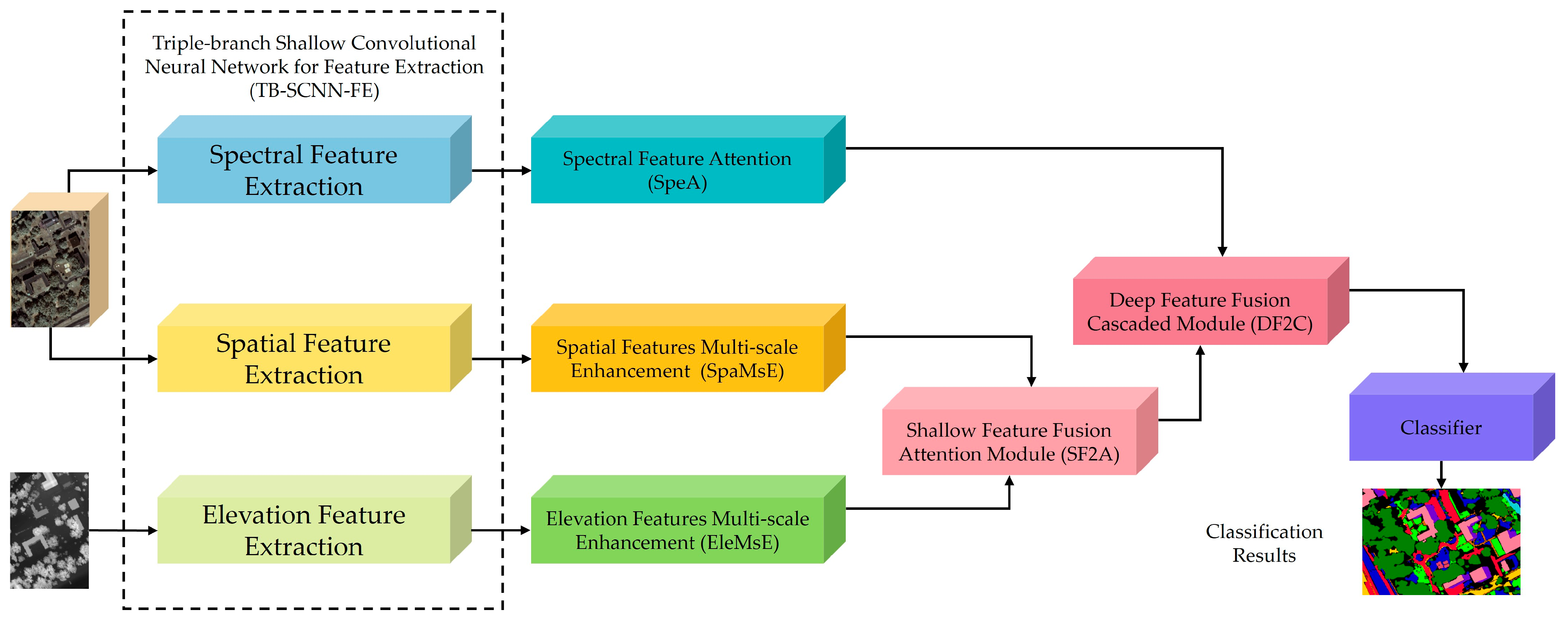
Based on the systematic analysis of MAHiDFNet [17] and the usage of the attention mechanism, the H-FANet put forward in this article retains the three-branch core architecture. Meanwhile, H-FANet introduces three key innovations to solve problems including rough spatial modeling, shallow fusion strategies, and insufficient training coordination.

FANet is reconstructed in terms of branch depth, feature enhancement, and fusion layer design. The shallow convolution of spatial branches and elevation branches has been reduced from the original four blocks to three blocks, reallocating computing resources to multi-scale modules and lowering the risk of overfitting. The spectral branches keep the same structure of two-layer one-dimensional convolution.

In this network, modality-specific multi-scale enhancement is adopted. In order to compensate for the neglect of texture scale and geometric gradient changes in the backbone network, SpaMsE (for HSI spatial branching) and EleMsE (for LiDAR elevation branching) implement convolutional splitting hierarchical aggregation paths for continuous textures and sparse elevations, respectively.

The hierarchical interaction strategy has been optimized. The Shallow Feature Fusion Attention Module (SF2A) only fuses the shape-related paths to guide geometric alignment. The spectral features are delayed to the Deep Feature Fusion Cascaded Module (DF2C) and are coupled with shape information through residual fusion. This optimization prevents early noise amplification and follows the principle of “geometry first, material later” in remote sensing.

The overall architecture has undergone systematic optimization in terms of internal modeling within branches, feature enhancement techniques, and fusion-path control. The H-FANet framework is composed of the modules shown in Figure 1.

Table A1. Detailed architecture of the proposed H-FANet.

Component	Parameter	Setting
Input	HSI patch size	$11\times 11\times B$ ($B=$ number of spectral bands)
	LiDAR patch size	$11\times 11\times 1$
	Patch radius (r)	5
Spectral Branch	Conv1D layers	2 blocks; $kernel=11$, $filters=64$; $kernel=3$, $filters=128$
	Pooling	MaxPool1D ($size=2$) after each Conv1D (except 1st)
	Activation	LeakyReLU ($\alpha =0.2$)
	Normalization	BatchNormalization
	Enhancement	SpeAE (self-attention + residual, coefficient $\gamma$)
Spatial Branch	Conv2D blocks (TB-SCNN-FE)	3 blocks; $filters=100$; $kernel=3\times 3, 3\times 3, 1\times 1$
	Activation	LeakyReLU ($\alpha =0.2$)
	Normalization	BatchNormalization
	Enhancement	SpaMsE (3 splits + 3 hierarchical fusions)
Elevation Branch	Conv2D blocks (TB-SCNN-FE)	3 blocks; $filters=100$; $kernel=3\times 3, 3\times 3, 1\times 1$
	Activation	LeakyReLU ($\alpha =0.2$)
	Normalization	BatchNormalization
	Enhancement	EleMsE (PyConv + EFR)
SpaMsE	Split operations	3 splits; kernels: $1\times 1$ and $3\times 3$
	Fusion operations	3 fusions; $kernel= 3\times 3$
	Output	Concatenation of enhanced + original features; $1\times 1$ Conv + BN + ReLU
EleMsE	Pyramid Convolution (PyConv)	3 parallel paths; kernels: $1\times 1$ (25 ch), $3\times 3$ (25 ch), $5\times 5$ (50 ch)
	Enhanced Feature Refinement (EFR)	ECA channel attention (Conv1D + sigmoid) + Spatial attention (Conv2D $7\times 7$ + sigmoid)
	Threshold	$\beta =0.2$
	Output	Concatenation of 3 refined paths
SF2A	Self-attention	3 Conv2D: {$Q$, $K$, $V$} per modality; Softmax attention map
	Cross-attention	$M_{ele}$ applied to spatial features; $M_{spa}$ applied to elevation features
	Coefficients	${\eta }_1$, ${\eta }_2$ (self-attention); ${\gamma }_1$, ${\gamma }_2$ (cross-attention)
	Weighted combination	${\alpha }_1+{\alpha }_2+{\alpha }_3=1$; ${\epsilon }_1+{\epsilon }_2+{\epsilon }_3=1$
DF2C	CNN processing	3 modality-specific CNNs: $F_{Dfus1-1}$, $F_{Dfus1-2}$, $F_{Dfus1-3}$
	Level-1 fusion	Details in Equations (8) and (9)
	Level-2 fusion	Details in Equation (10)
Classification	FC layers	Dense (1024, ReLU) → Dropout (0.4) → Dense (512, ReLU) → Dropout (0.4)
	Output layer	Dense ($C$, softmax), $C =$ number of classes

summarizes the model input configuration and the architectural details of each branch and module. All convolutional layers use stride = 1 with ‘same’ padding for 2D convolutions and ‘valid’ padding for 1D convolutions, unless otherwise specified.

3.1. Three-Branch Shallow Convolutional Feature Extraction Module TB-SCNN-FE

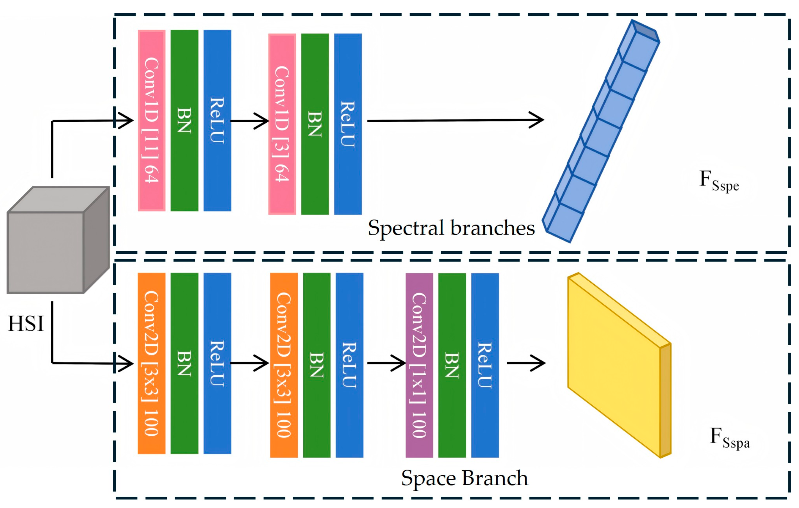
When designing H-FANet, it follows the basic principle of decoupling and extracting tri-modal features: spectral, spatial, and elevation. It uses three independent ways to process the input data corresponding to each mode, as shown in Figure 2.

The spectral branch processes the spectral signature associated with each pixel using two one-dimensional convolutional blocks. Its output is denoted by $F_{Sspe}$. The HSI spatial branch models the local spatial neighborhood, and its output is denoted by $F_{Sspa}$. For each target pixel $P_{ij}$, an HSI patch centered at $P_{ij}$ with a spatial radius $r$ is extracted as the input to the spatial branch, resulting in a patch size of $\left(2r+1\right)\times \left(2r+1\right)$.

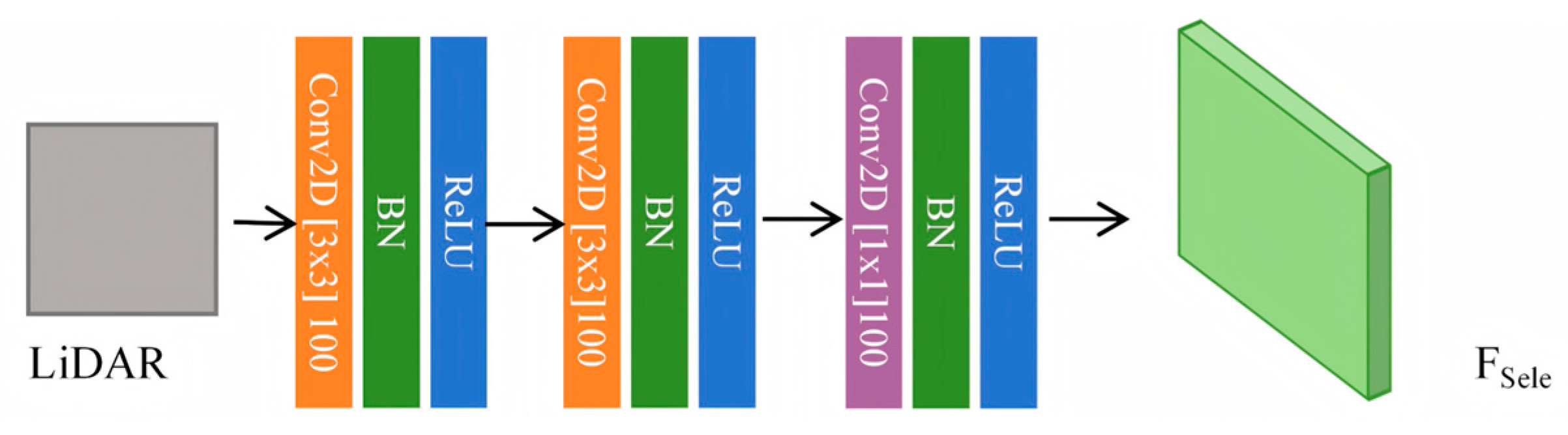
As shown in Figure 3, the path for shallow feature extraction of the LiDAR input is composed of the elevation branch.

The elevation branch processes the LiDAR elevation image to extract spatial geometric features, including terrain and structural information. Its output is denoted by $F_{Sele}$.

In the spatial branch and elevation branch, H-FANet reduces the original four-layer shallow convolutional blocks of MAHiDFNet [17] to three layers. This modification is based on two main considerations. First, due to the introduction of dedicated structural enhancement modules (SpaMsE and EleMsE) for each branch by H-FANet, its multi-scale modeling capability has been improved. To prevent excessive parameter redundancy or feature overfitting in lower layers, it is reasonable to decrease the number of convolutional layer stacks. Second, shallow feature extraction networks may encounter problems like information degradation or gradient dissipation, considering that remote sensing tasks are usually carried out with limited training samples. By moderately compressing the initial network depth, the computational cost can be effectively controlled while maintaining the representation ability of basic features. This structural adjustment enables the architecture budget to be distributed more effectively to subsequent modules without affecting the performance of basic feature extraction.

3.2. Spectral Feature Attention Module SpeA

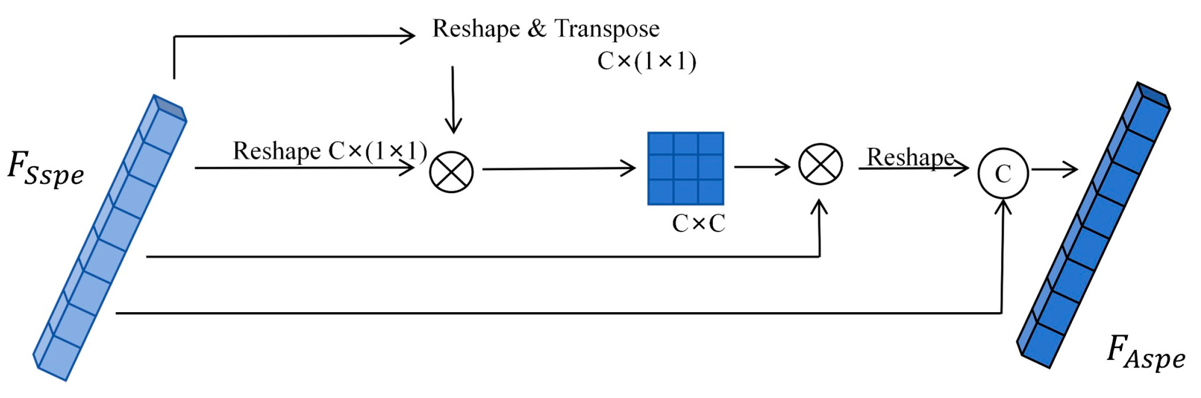
The attention mechanism can automatically allocate weights based on the importance of information, highlighting vital features. In this paper, the spectral attention module adopted the design in reference [14], and its detailed architecture is illustrated in Figure 4.

As shown in Figure 4, $F_{Sspe}$ denotes the shallow spectral feature, while $F_{Aspe}$ denotes the attention-enhanced spectral feature.

3.3. Multi-Scale Spatial Enhancement Module (SpaMsE)

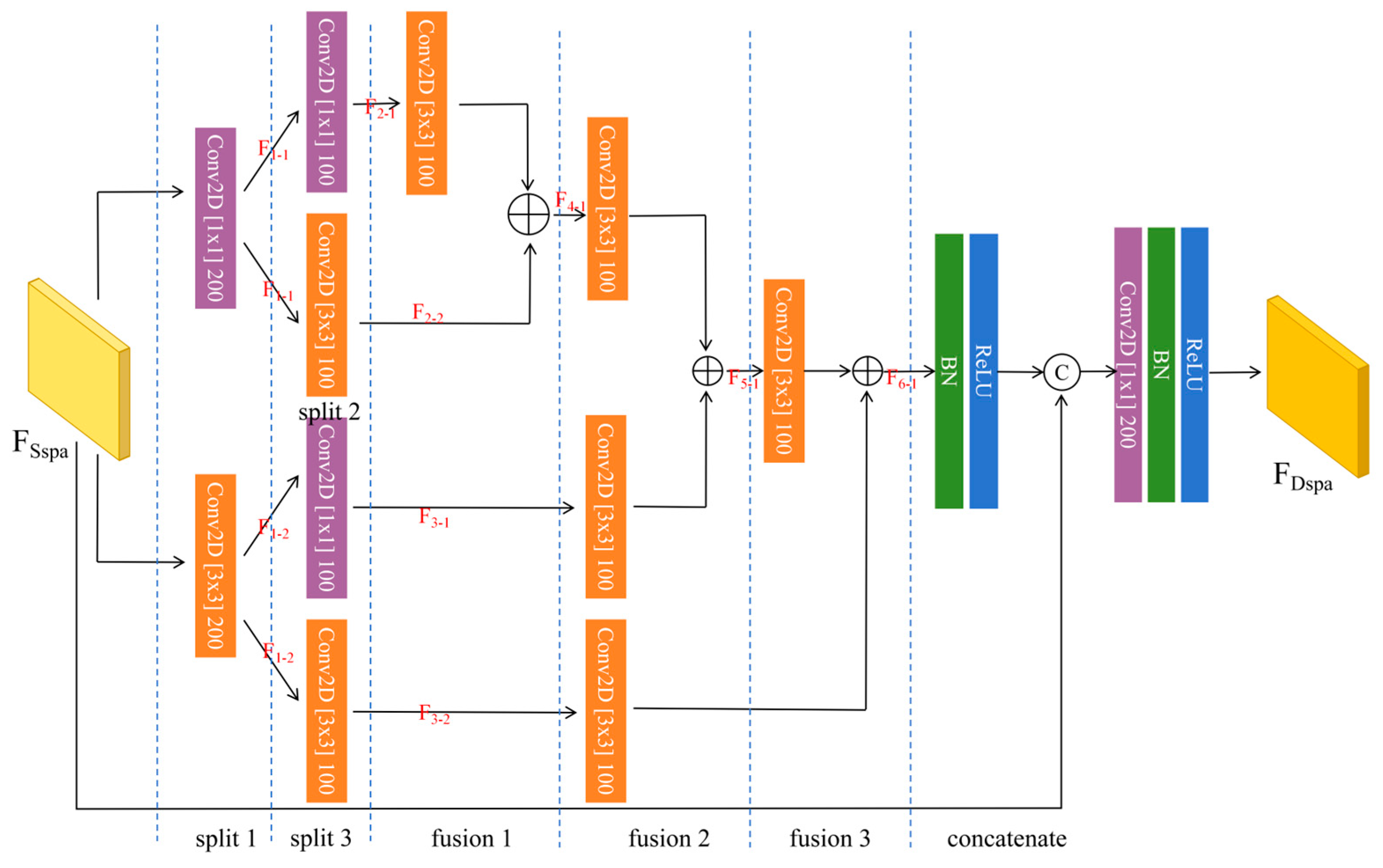
To capture spatial patterns at different scales in hyperspectral images, we propose the Multi-scale Spatial Enhancement Module (SpaMsE), whose architecture is illustrated in Figure 5. Land-cover objects may exhibit substantial variations in size, shape, and spatial arrangement within the same scene. For example, tree crowns may appear as small isolated objects in one region but form large continuous canopies in another. Consequently, a single fixed receptive field may be insufficient to represent both fine-grained textures and broader contextual structures [29].

Given the shallow spatial feature $F_{Sspa}$, SpaMsE applies three convolutional split operations to generate four scale-specific feature maps with progressively enlarged receptive fields. The split process is compactly expressed as Equation (1):

$$\left\{F_{s1},F_{s2},F_{s3},F_{s4}\right\}=\mathcal{S}\left(F_{Sspa}\right)$$

(1)

where $\mathcal{S}\left(\cdot \right)$ denotes the hierarchical convolutional split operation, and $F_{s1}, F_{s2}, F_{s3}, F_{s4}$ represent spatial features at different receptive-field scales. Features with relatively small receptive fields preserve local textures and boundary details, whereas features with larger receptive fields encode broader spatial structures and contextual information.

The resulting multi-scale features are progressively integrated through three hierarchical fusion operations. The fusion process is defined as Equation (2):

$$\begin{array}{c}{G}_1={\varphi }_1\left(F_{s1}\right)+F_{s2}\\ G_2={\varphi }_2\left(G_1\right)+F_{s3}\\ G_3={\varphi }_3\left(G_2\right)+F_{s4}\end{array}$$

(2)

where ${\varphi }_i\left(\cdot \right)$ denotes the convolutional transformation used at the i-th fusion stage, and $G_i$ represents the corresponding fused feature. This progressive aggregation allows information from adjacent receptive-field levels to interact hierarchically.

Although the hierarchically fused feature contains enhanced multi-scale information, directly using it may weaken some low-level spatial details. Therefore, the original shallow spatial feature is retained through a concatenation connection. The final output of SpaMsE is formulated as Equation (3):

$$F_{Dspa}={\varphi }_{\mathrm{o}\mathrm{u}\mathrm{t}}\left(\mathit{Concat}\left[F_{Sspa},G_3\right]\right)$$

(3)

where $Concat\left[\cdot \right]$ denotes channel-wise concatenation and ${\varphi }_{\mathrm{o}\mathrm{u}\mathrm{t}}\left(\cdot \right)$ denotes the final convolutional transformation. The resulting feature $F_{Dspa}$ combines fine-grained spatial details from the original shallow representation with the broader contextual information obtained through hierarchical multi-scale fusion. The complete layer configuration of SpaMsE is summarized in Table A1.

3.4. Multi-Scale Elevation Feature Enhancement Module (EleMsE)

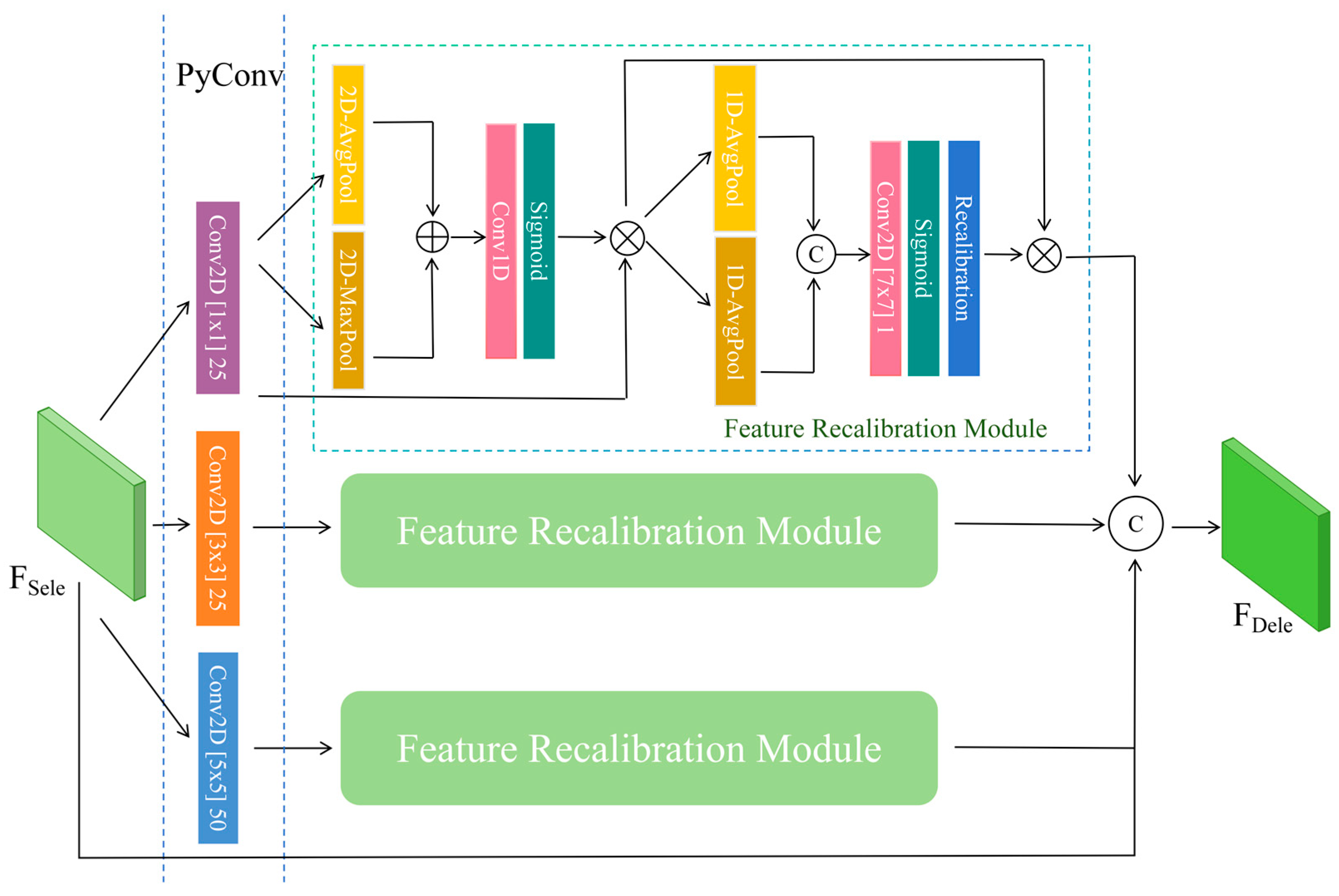
In LiDAR data, the elevation changes of terrain and objects may exhibit different patterns at different scales. In addition, there may be spatial differences in point cloud density, resulting in inconsistent feature resolutions. Facing these challenges, this section introduces the Elevation Feature Multi-Scale Enhancement Module (EleMsE), whose architecture is illustrated in Figure 6.

Considering that pyramid convolution is able to adapt to LiDAR data with different resolutions and densities, as shown in the pyramid convolution (PyConv) module on the left side of Figure 6, this section will adopt three sets of PyConv for extracting multi-scale elevation features. A $1\times 1$ kernel, for instance, responds well to abrupt transitions like building rooftops and road edges; a $3\times 3$ kernel is better suited to gradual terrain relief; while a $5\times 5$ kernel can reach out far enough to encode the layout of an entire block or neighborhood.

After that, we apply the Elevation Feature Enhancement Module (EleFE). This module has both the advantages of efficient channel attention [30] and spatial attention [31]. It optimizes spatial feature distribution and channel weights, which boosts the feature representation capability. This module is applied at each scale to enhance the ability to express features. Eventually, these enhanced features are fused to capture local details and global structural information. The final output $F_{Dele}$ combines the original feature map with the enhanced feature map to keep the underlying details.

In the first stage of the EleFE module, the input feature map $F$ undergoes parallel processing via average pooling (denoted as $2DAvg$) and max pooling (denoted as $2DMax$) along the spatial dimensions, followed by element-wise addition. Subsequently, the resulting tensor passes through a one-dimensional convolutional layer with a sigmoid activation function and finally undergoes element-wise multiplication with the input feature map $F$. The output of the first stage is denoted as $F_1$, with its mathematical expression shown in Equation (4):

$$F_1=F⨂sigmoid\left(Conv1D\left(2DAvg\left(F\right)+2DMax\left(F\right)\right)\right)$$

(4)

In the second stage of EleFE, the output from the first stage is processed in parallel through the channel-wise average pooling layer (denoted as $1DAvg$) and the channel-wise maximum pooling layer (denoted as $1DMax$), followed by a concatenation operation. Subsequently, the concatenated result is passed through a two-dimensional convolutional layer and a sigmoid activation layer. The resulting weight matrix of the second stage is denoted as $M_2$, as defined in Equation (5):

$$M_2=sigmoid\left(Conv2D\left(concatenate\left[1DAvg\left(F_1\right),1DMax\left(F_1\right)\right]\right)\right)$$

(5)

A calibration module is subsequently incorporated to preserve those pixels with a higher probability of having the same label as the central pixel, as defined by Equation (6):

$$\begin{array}{cc} M_{2,ij}=M_2,& M_{2,ij}\ge \beta \\ M_{2,ij}=0,& M_{2,ij}<\beta \end{array}$$

(6)

In the above formula, $\beta$ is the threshold for determining whether the pixel label is likely to be like the center pixel. The threshold $\beta$ is set to 0.2 to filter out weak spatial attention responses. This value retains spatial locations with meaningful attention weights while suppressing near-zero responses that contribute little to feature refinement.

The final two-stage output $F_{Dele}$ can be calculated using Equation (7):

$$F_{Dele}=M_2⨂F_1$$

(7)

3.5. SF2A

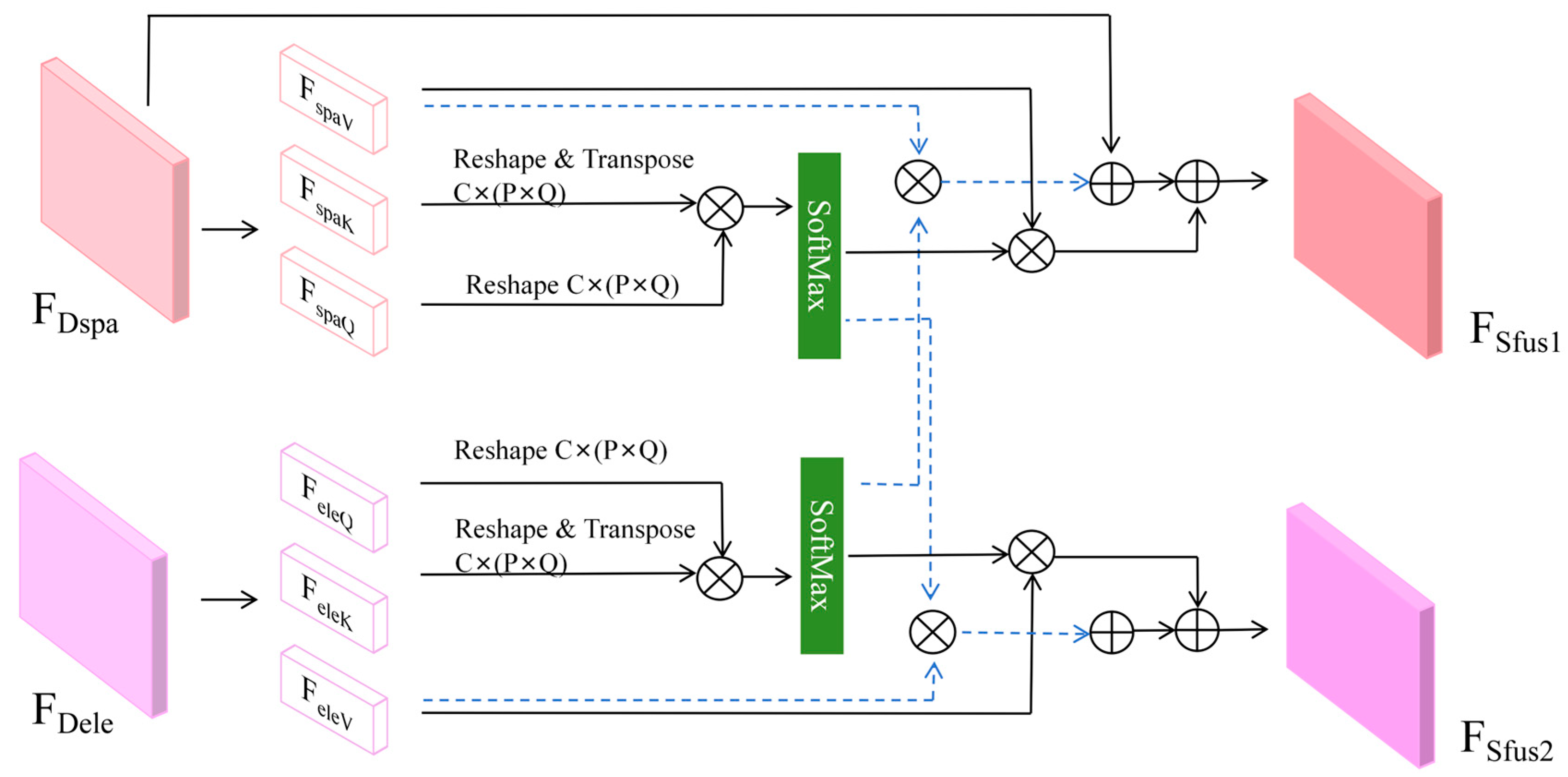
Basic cross-attention [32] enables dynamic focus on correlations between different modalities, and feature fusion integrates this information to improve feature discrimination capabilities. The shallow feature fusion method employed in this network fully exploits the interdependencies among multimodal data and incorporates a modal attention module for HSI-LiDAR fusion to improve fusion accuracy, as illustrated in Figure 7.

The SF2A module performs lightweight cross-attention only between the HSI-Spatial and LiDAR-Elevation pathways at a shallow level, enabling rapid alignment of geometric scales, while the spectral branch bypasses this stage entirely. This is because shallow features retain precise spatial contours, making them more suitable for pixel-level geometric alignment between texture-defined and height-defined boundaries before semantic divergence occurs in deeper layers. Algorithm 1 outlines the data processing steps.

Algorithm 1. Shallow feature fusion
Step	Operate	HSI-Spatial Branch	LiDAR-Elevation Branch
1	Q/K/V Projection	$Q_{spa},K_{spa},V_{spa}\leftarrow Conv(F_{Dspa})$	$Q_{ele},K_{ele},V_{ele}\leftarrow Conv\left(F_{Dele}\right)$
2	Self-Attention	$M_{spa}=Softmax(Q_{spa}\cdot K_{spa}^T)$	$M_{ele}=Softmax(Q_{ele}\cdot K_{ele}^T)$
		$F_{Aspa}={{\eta }_{1}M}_{spa}·V_{spa}$	$F_{Aele}={{\eta }_{2}M}_{ele}·V_{ele}$
3	Shape cross fusion	$F_{Mspa}={{\gamma }_{1}M}_{ele}·V_{spa}$	$F_{Mele}={{\gamma }_{2}M}_{spa}·V_{ele}$
4	Three Features Weighted Aggregation	$F_{Sfus1}={\alpha }_1{F}_{Dspa}+{\alpha }_2{F}_{Aspa}+{\alpha }_3{F}_{Mspa}$	$F_{Sfus2}={\epsilon }_1{F}_{Dele}+{\epsilon }_2{F}_{Aele}+{\epsilon }_3{F}_{Mele}$

In the SF2A module, the network initially receives texture shape features $F_{Dspa}$ from the SpaMsE and geometric elevation features $F_{Dele}$ from the EleMsE. These features are mapped into query, key, and value tensors through convolutional operations. For the spatial branch, they were denoted as $Q_{spa}$, $K_{spa}$, and $V_{spa}$. For the elevation branch, they were denoted as $Q_{ele}$, $K_{ele}$, and $V_{ele}$. And all of them enabled the computation of position-to-position attention matrices $M_{spa}$ and $M_{ele}$. The pure attention features $F_{Aspa}$ and $F_{Aele}$ are then derived by scaling the attention outputs with factors ${\eta }_1$ and ${\eta }_2$.

Subsequently, adaptive combination coefficients ${\gamma }_1$ and ${\gamma }_2$ are applied to integrate the dual-branch features in a cross-adaptive manner, generating “shape-enhanced” features $F_{Mspa}$ and $F_{Mele}$ to facilitate early geometric alignment. Finally, within each branch, the original features, pure attention features, and shape-enhanced features are linearly combined using weights ${\alpha }_1~{\alpha }_3$ and ${\epsilon }_1~{\epsilon }_3$, yielding two shallow outputs $F_{Sfus1}$ and $F_{Sfus2}$. These “shape-first” features are later fused with the spectral branch’s semantic vectors in the deep DF2C module, thereby completing the hierarchical fusion strategy of H-FANet.

Compared to three-way multi-head early fusion approaches, SF2A offers advantages including fewer parameters, reduced computational time, and the mitigation of early spectral noise diffusion. This design also preserves sufficient cross-modal mutual information for effective processing in the subsequent DF2C stage.

3.6. DF2C

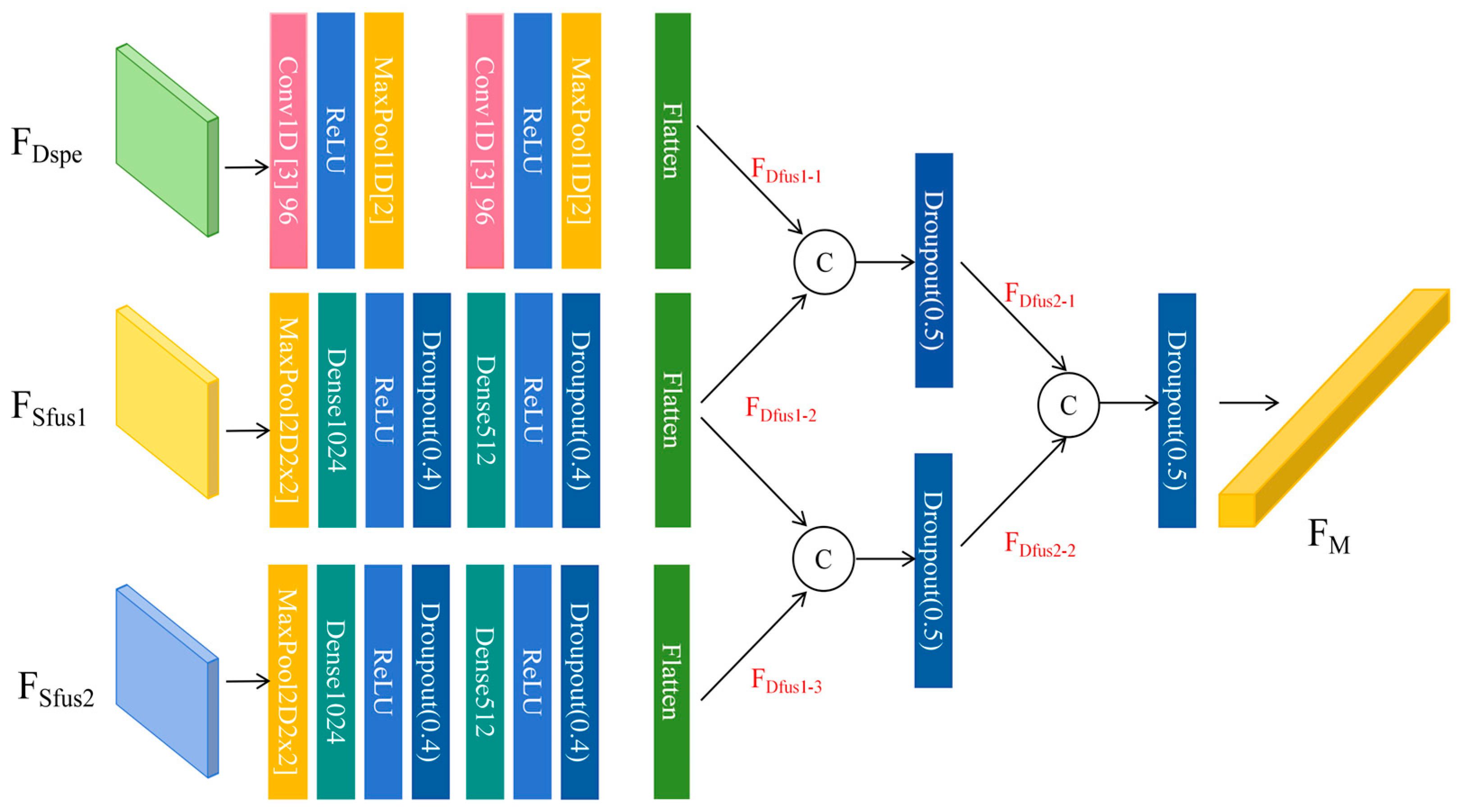
Feature $F_{Aspe}$ is obtained through the spectral feature attention module SpeA, and $F_{Sfus1}$ and $F_{Sfus2}$ are obtained through the shallow feature attention fusion module SF2A. In the deep feature fusion cascade module DF2C, the above three features are respectively input into three different CNNs to prepare for the subsequent cascade fusion operation. Such a two-level cascade mirrors the hierarchical land cover interpretation process: first associating geometric forms with material identities, then refining cross-modal semantics while preserving modality-specific information through residual connections. The output features are $F_{Dfus1-1}$, $F_{Dfus1-2}$ and $F_{Dfus1-3}$. The left side of Figure 8 shows the specific layer structure.

The first-level deep fusion process is described by Equations (8) and (9). Among them, $F_{Dfus2-1}$ and $F_{Dfus2-2}$. These are the output features of the first level of deep fusion.

$$F_{Dfus2-1}=Dropout\left(0.5\right)\left(concatenate\left[F_{Dfus1-1},F_{Dfus1-2}\right]\right)$$

(8)

$$F_{Dfus2-2}=Dropout\left(0.5\right)\left(concatenate\left[F_{Dfus1-2},F_{Dfus1-3}\right]\right)$$

(9)

The second-level deep fusion process is described by Equation (10), where $F_M$ denotes the final fusion feature of H-FANet.

$$F_M=Dropout\left(0.5\right)\left(concatenate\left[F_{Dfus2-1},F_{Dfus2-2}\right]\right)$$

(10)

3.7. Classification Module and Loss Function

The classification and loss function modules in this study adopt the same configuration as MAHiDFNet [17]. This decision is primarily motivated by the fact that the model optimization in this work focuses on enhancing feature extraction methods and feature fusion pathways, rather than modifying the classification or loss function components. To ensure a fair comparison and enable effective evaluation of subsequent performance, the design of these modules is retained without alteration.

The workflow of the classification module is as follows. The final fusion features from each modality are concatenated; the concatenated representation is compressed through a fully connected layer, and then the Softmax activation function is applied to generate classification probability predictions pixel-by-pixel. The formal expression of this process is provided in Equation (11):

$$\begin{array}{c}{F}_m=f\left(W\cdot F_M+b\right)\hfill \\ {\mathit{pred}\left(i,j\right)}_k={\displaystyle \frac{exp\left({\theta }_k\mid F_{m,ij}\right)}{{\displaystyle {\sum }_{c=1}^K} \exp \left({\theta }_c\mid F_{m,ij}\right)}}, k=\mathrm{1,2},\dots ,K\hfill \end{array}$$

(11)

In the equation, $W$ and $b$ represent the weight matrix and bias term of the fully connected layer, respectively, $k$ denotes the class index, $c$ is the summation index running over all $K$ classes, and $K$ is the total number of feature categories. The output $pred(i,j)$ represents the predicted category probability value of the position $(i,j)$.

To avoid the common category imbalance problem in remote sensing scenes, the loss function adopts weighted cross-entropy loss. Its definition is shown in Equation (12):

$${\mathcal{L}}_{W-C}=-{\displaystyle \frac{1}{U}}{\displaystyle \sum _{n=1}^U} {\displaystyle \sum _{j=1}^K}{\omega }_j\log \mathrm{Pr}\left(Y^n=j\mid \left(X_H^n,X_L^n\right);\theta \right),{\omega }_j={\displaystyle \frac{U}{K\cdot n_j}}$$

(12)

Among them, ${\omega }_j$ is the weight of the j-th class, which is determined based on class frequency. $U$ is the total number of training samples. Based on the consistency of classification and loss functions, this research can concentrate more on evaluating the strengths of new feature-extraction methods and fusion paths, as well as the performance improvements they bring.

4. Datasets and Experimental Setting

4.1. Experimental Dataset

To evaluate how the proposed network performs, three public datasets are adopted in this paper: Trento [18], Houston 2013 [19] and Muufl Gulfport [20].

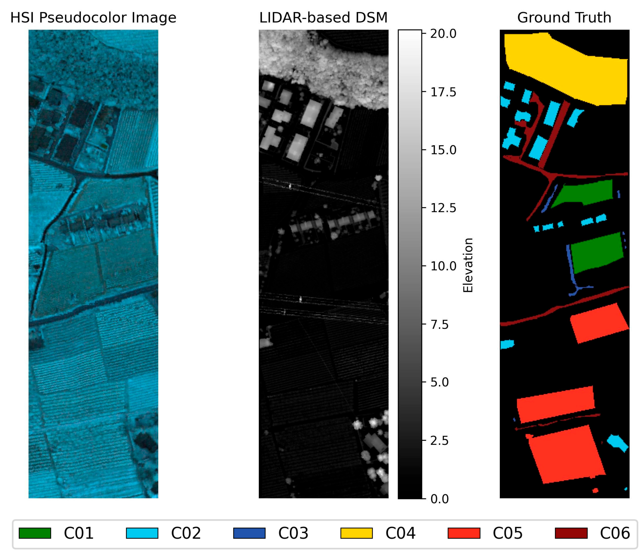
The Trento dataset was collected in a rural area in the south of Trento, Italy. The LiDAR data was collected by the Optech ALTM 3100EA sensor (Teledyne Optech, Vaughan, ON, Canada), while the HSIs were captured by the AISA Eagle sensor (Specim, Oulu, Finland), containing a total of 63 spectral bands. The spatial dimensions of both types of data are 166 × 600 pixels, with a 1 m spatial resolution.

Table 1. The number of training and testing samples for each category in the Trento dataset.

Category Number	Category Name	Number of Training Samples	Number of Test Samples
01	Apple Orchard	100	3934
02	Building	100	2803
03	Corn Field	100	379
04	Forest	100	9023
05	Vineyard	100	10,401
06	Road	100	3274
-	Overall	600	29,814

presents the number of samples across six distinct categories.

To facilitate the understanding of the characteristics of this experimental dataset, Figure 9 shows the pseudo-color synthesized HSI, the grayscale LiDAR data, and the color labels corresponding to different object types. The pseudo-color synthesized HSI image is created using bands 40, 50, and 60.

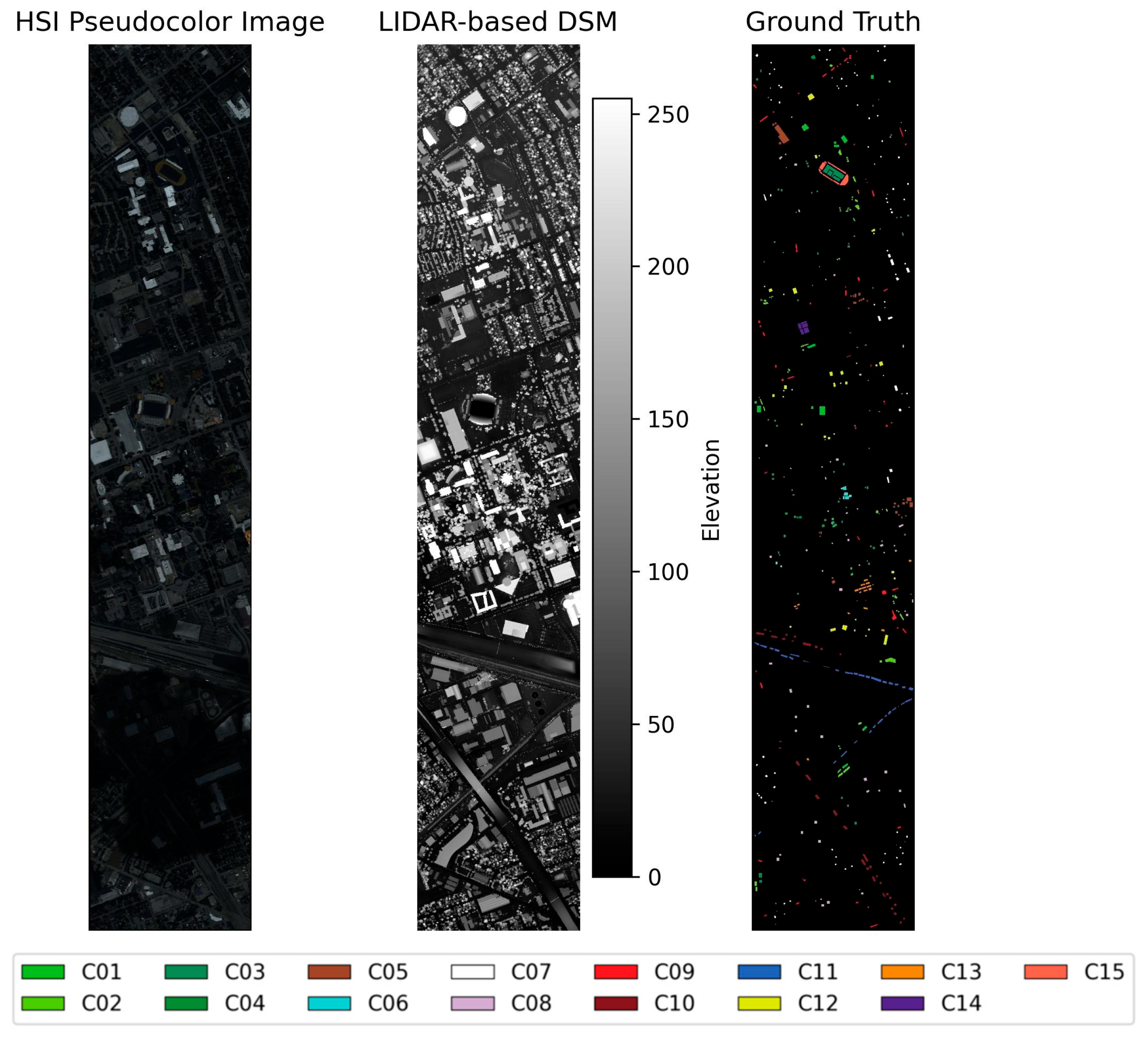
The Houston 2013 dataset comprises HSI and LiDAR data, and both of these data categories have a pixel dimension of 349 × 1905 and a spatial resolution of 2.5 m. The HSI data contains 144 spectral bands, and the dataset includes samples from 15 distinct land cover categories.

Table 2. The number of training and testing samples for each category in the Houston 2013 dataset.

Category Number	Category Name	Number of Training Samples	Number of Test Samples
01	Healthy Grass	100	1151
02	Damaged Grass	100	1154
03	Artificial Grass	100	597
04	Trees	100	1144
05	Bare Land	100	1142
06	Water Body	100	225
07	Residential Area	100	1168
08	Commercial Area	100	1144
09	Road	100	1152
10	Highway	100	1127
11	Railway	100	1135
12	Parking Lot 1	100	1133
13	Parking Lot 2	100	369
14	Tennis Court	100	328
15	Running Track	100	560
-	Overall	1500	13,529

presents the number of training and test samples for the 15 categories in the dataset.

Figure 10 presents the pseudo-color-synthesized HSI image, the grayscale LiDAR data image, and the color-coded labels representing different object types. The pseudo-color-synthesized HSI image is constructed using bands 40, 50, and 60.

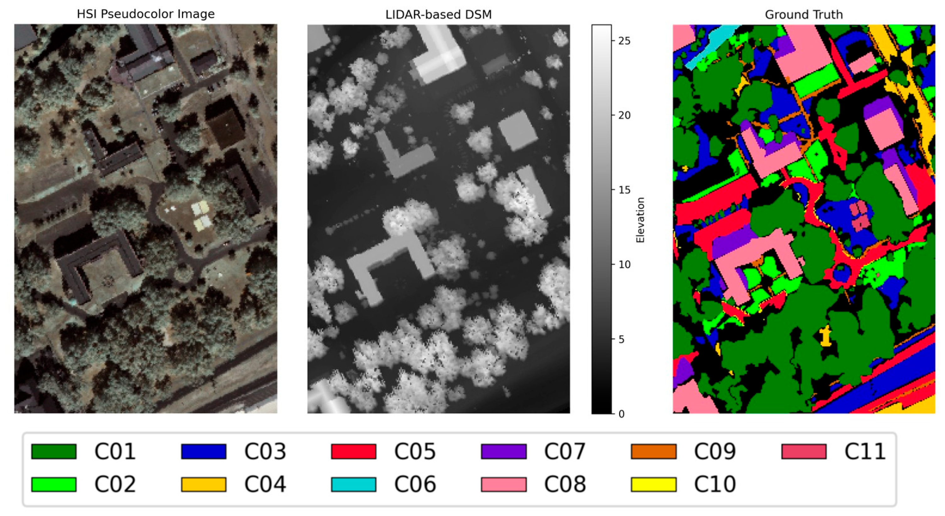
The Muufl Gulfport dataset contains hyperspectral images with pixel sizes of 325 × 220 and 72 spectral bands. The corresponding LiDAR images contain elevation data from two rasters. To mitigate noise effects, the first 8 spectral bands and the final 8 ones were excluded, which left us with a total of 64 usable spectral bands. The dataset represents 11 urban land cover classes.

Table 3. The number of training and testing samples for each category in the Muufl Gulfport dataset.

Category Number	Category Name	Number of Training Samples	Number of Test Samples
01	Trees	100	23,146
02	Pure Grass Cover	100	4170
03	Mixed Surface	100	6782
04	Bare Ground	100	1726
05	Road	100	6587
06	Water body	100	366
07	Building Shadow	100	2133
08	Building	100	6140
09	Sidewalk	100	1285
10	Yellow Curb Strip	100	83
11	Fabric Panel	100	169
-	Overall	1100	52,587

presents the number of training and test samples for 11 categories in the Muufl Gulfport dataset.

Figure 11 presents the pseudo-color synthesized HSI image, the grayscale LiDAR data image, and the color-coded labels corresponding to each ground object type. The pseudo-color synthesized HSI image is derived from bands 40, 50, and 60.

Both the HSI and LiDAR data were normalized using Z-score standardization prior to training. Pixels with zero labels (background or unlabeled) were excluded from sampling.

4.2. Evaluation Metrics

In remote sensing image classification tasks, four evaluation indicators are commonly employed [33]: overall classification accuracy, classification accuracy for each category, average classification accuracy across categories, and the Kappa coefficient. This study utilizes these four metrics, with their formal definitions provided in Equations (13)–(16):

(1)

Overall accuracy (OA)

$$OA={\displaystyle \sum _{i=1}^c}{\displaystyle \frac{N_{ii}}{N}}$$

(13)

(2)

Class accuracy (CA)

$$CA={\displaystyle \frac{N_{ii}}{N_i}}$$

(14)

(3)

Average accuracy (AA)

$$AA={\displaystyle \frac{1}{K}}{\displaystyle \sum _{i=1}^K}C{A}_i={\displaystyle \frac{1}{K}}{\displaystyle \sum _{i=1}^K}{\displaystyle \frac{N_{ii}}{N_i}}$$

(15)

(4)

Kappa coefficient

$$\mathit{Kappa} ={\displaystyle \frac{N{\displaystyle {\sum }_{i=1}^K}{N}_{ii}-{\displaystyle {\sum }_{i=1}^K}\left(N_{i+}\times N_{+i}\right)}{N^2-{\displaystyle {\sum }_{i=1}^K}\left(N_{i+}\times N_{+i}\right)}}$$

(16)

Among them, $N$ represents the total quantity of samples; $K$ denotes the overall quantity of categories; $N_{ii}$ denotes the number of samples in the i-th class that were correctly classified; $N_i$ represents the total number of true samples of i-th class; $N_{i+}$ denotes the total count of row i in the confusion matrix (the true category is the i-th class); $N_{+i}$ denotes the total count of column i of the confusion matrix (the predicted category is the i-th class).

4.3. Experimental Setup and Comparison Models

In this experiment, Python 3.8 and CUDA 10.1 were used to implement the program, and TensorFlow 2.3.2 was employed to construct the convolutional neural network. The server is equipped with an Intel(R) Xeon(R) CPU E5-2699 v4 and a GPU with 8 GB of memory. In the H-FANet designed in this study, the spatial size of the input features is set to $11 \times 11$.

Glorot uniform initialization was adopted for all convolutional and fully connected layers. During training, 80% of the training samples were held out for training and 20% for validation. The checkpoint achieving the lowest validation loss was retained as the final model. No early stopping mechanism was applied. To ensure a fair comparison, all competing models were re-implemented under the same experimental conditions, using the same data splits and evaluation protocol. Each model was independently trained five times with different random seeds for parameter initialization. The training, validation, and test splits remained the same across all runs. Results are reported as mean ± standard deviation. With fixed data splits, the variation comes only from training randomness such as weight initialization, data shuffling order, and dropout patterns. Further details are provided in

Table 4. Experimental parameter configuration.

Parameters	Configuration Values
Input size (r)	5
Batch size	64
Number of training iterations (epoch)	100
Number of training samples for each category	100
Optimizer	Adam
Learning rate decay rate	0.99
Initial learning rate	0.0001

.

To evaluate the fusion classification performance of the method proposed in this study, this section compares the proposed network with five existing advanced multimodal fusion classification methods through classification accuracy and visualization results on three datasets: Trento, Houston 2013, and Muufl Gulfport.

Table 5. Comparison model description.

Method	Architecture	Fusion Mechanism	Attention Design
EndNet (2019) [21]	Two-stage sparse CNN Auto Encoder	Early feature-level fusion inside the encoder	No explicit attention: loss combines SAD + KL for endmember separation
MAHiDFNet (2022) [17]	Triple branch CNN (HSI Spectral/HSI Spatial/LiDAR)	Shallow Modality Attention, deep concatenation	Custom Modality Attention + Self-Attention modules
GLT Net (2021) [25]	Hybrid Multi-scale CNN + ViT	Multi-scale CNN local fusion; ViT global spectral modeling; decision-level weighted fusion;	ViT encoder–decoder does multi-head spectral MSA; CNN side uses SA GDR attention
MFT (2023) [20]	Pure Vision Transformer encoder	HSI patch tokens + LiDAR CLS tokens interact inside the encoder	mCross Patch Attention-LiDAR CLS as Query, HSI patch as Key/Value
Cross HL (2024) [26]	Pure ViT	Feature level via the Cross-HL module	Cross HL Attention-LiDAR Query × HSI Key/Value

provides a concise summary of the design characteristics of the models compared:

To achieve a fair and transparent comparison, all five competing models were re-implemented and re-trained under the same experimental conditions and data splitting scheme. The remaining labeled samples constituted the test set. For each selected sample, an $11 \times 11$ patch centered on the target pixel was extracted as the model input. This random sampling strategy follows the widely adopted protocol in patch-based hyperspectral classification studies.

5. Results

5.1. Comparative Evaluation of Classification Effect

5.1.1. Classification Performance on the Trento Dataset

The classification performance of various models on the Trento dataset was quantitatively compared with the results shown in

Table 6. Performance comparison of different models on the Trento Dataset (%).

Category No.	Category Name	EndNet	MAHiDFNet	MFT	GLT-Net	Cross-HL	H-FANet
01	Apple Orchard	96.24 ± 0.37	96.95 ± 0.33	96.61 ± 0.22	99.88 ± 0.12	98.86 ± 0.45	96.47 ± 0.11
02	Building	94.79 ± 0.40	96.33 ± 0.40	87.76 ± 0.42	94.75 ± 0.22	97.12 ± 0.22	99.90 ± 0.08
03	Corn Field	81.16 ± 0.56	98.41 ± 0.20	97.63 ± 0.34	89.16 ± 0.43	71.72 ± 0.49	98.58 ± 0.12
04	Forest	99.92 ± 0.06	99.93 ± 0.04	99.88 ± 0.07	99.90 ± 0.03	99.88 ± 0.02	99.95 ± 0.03
05	Vineyard	81.53 ± 0.72	93.89 ± 0.31	81.91 ± 0.62	94.74 ± 0.12	89.05 ± 0.43	99.68 ± 0.21
06	Road	91.99 ± 0.47	89.778 ± 0.38	90.04 ± 0.53	98.53 ± 0.30	98.84 ± 0.32	97.68 ± 0.12
OA ↑		91.42 ± 0.32	95.96 ± 0.08	90.93 ± 0.26	97.33 ± 0.05	95.24 ± 0.19	99.13 ± 0.06
AA ↑		90.94 ± 0.29	95.88 ± 0.07	92.31 ± 0.23	96.16 ± 0.14	92.58 ± 0.13	98.71 ± 0.04
Kappa ↑		88.54 ± 0.43	94.660 ± 0.11	87.88 ± 0.35	96.43 ± 0.07	93.63 ± 0.26	98.83 ± 0.09

↑ indicates that higher values denote better performance.

. The proposed H-FANet network obtains the highest OA, AA, and Kappa values.

Specifically, the OA value obtained is 99.13 ± 0.06%, the AA value is 98.71 ± 0.04%, and the Kappa coefficient is 98.83 ± 0.09% in H-FANet. The OA indicates that a large percentage of samples were classified correctly across the dataset. The AA reflects strong classification performance for both minority and majority classes. The Kappa coefficient demonstrates a high level of agreement between the predicted labels and true labels.

Collectively, these experimental results validate the reliability of the proposed model when performing fusion classification on this dataset. In contrast, the OA, AA, and Kappa metrics of the CNN-based encoder-decoder network EndNet are significantly decreased, and its overall performance is inferior to that of all other models. Its OA is only 91.42 ± 0.32%, which is approximately 7.71% lower than that of the H-FANet proposed in this paper. The main reason for this performance gap lies in the fact that the model in this paper fully utilizes the modeling ability of the Attention mechanism for sequential relationships. Despite its relatively low overall performance, EndNet still achieved a 99.92 ± 0.06% classification accuracy in the forest category, indicating that the current CNN-based fusion methods still have potential for further improvement.

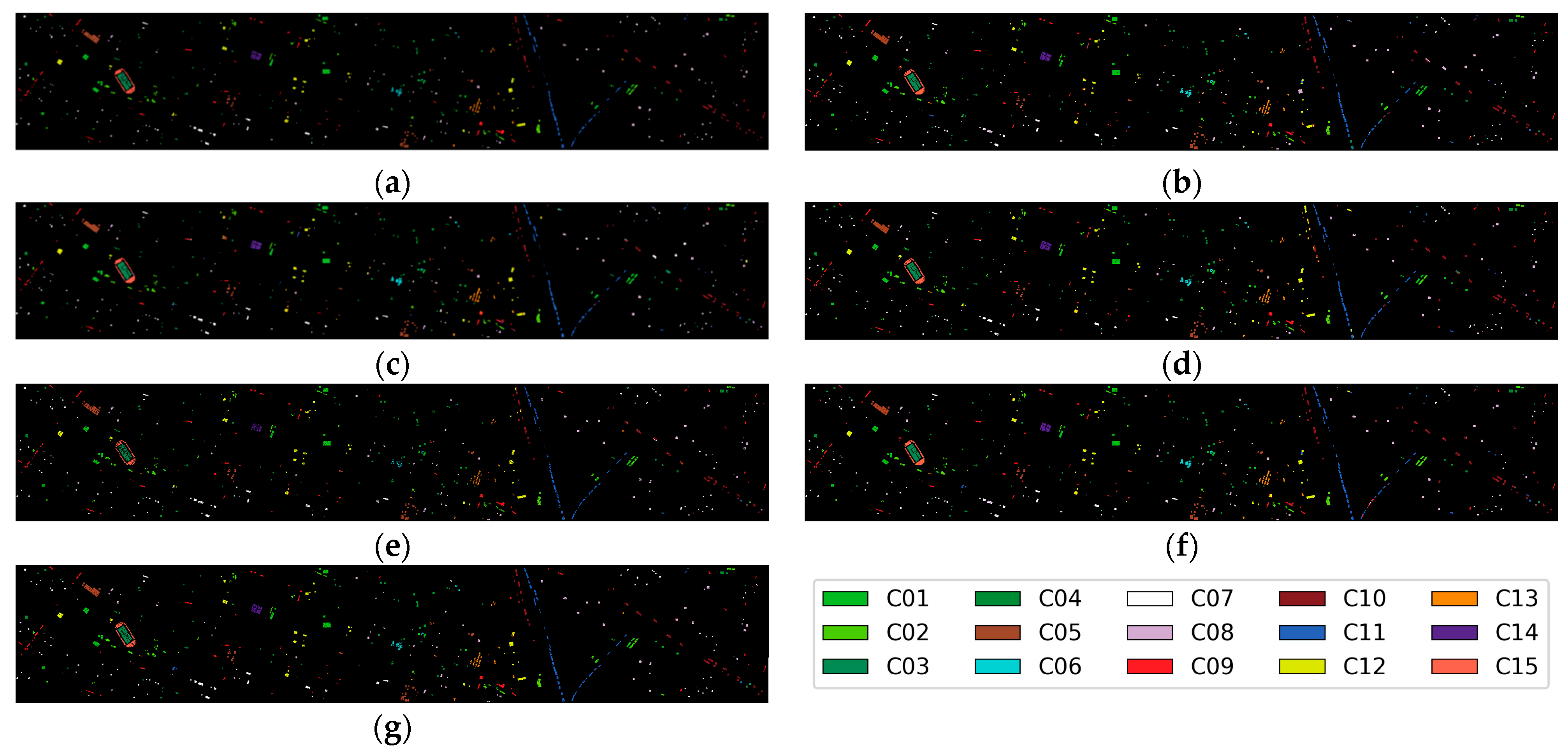
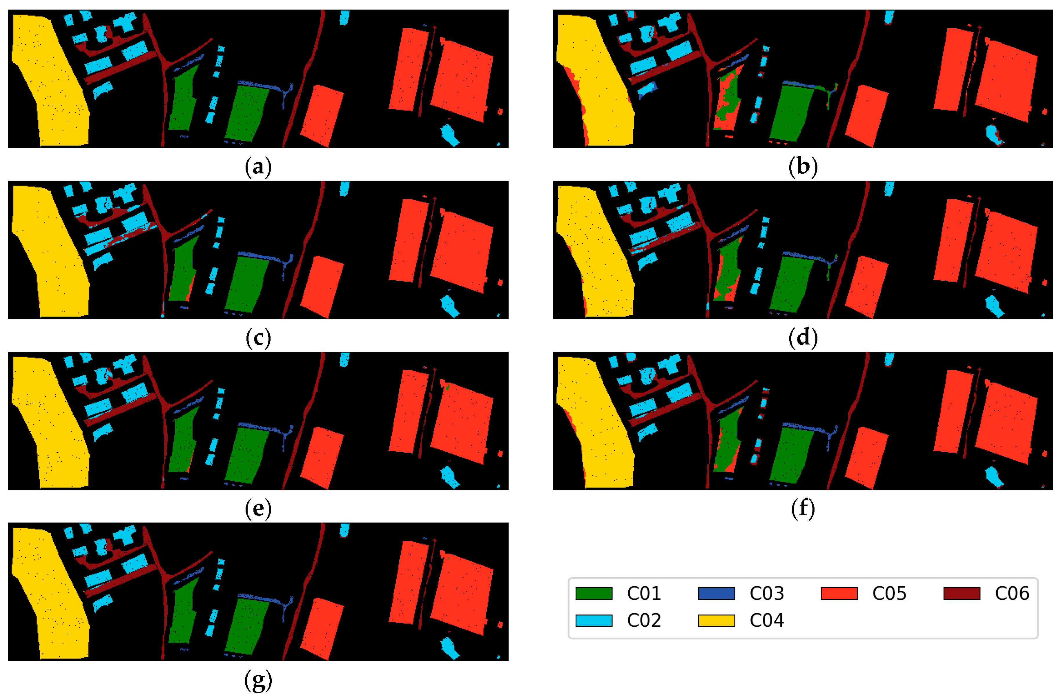
Figure 12 shows the visual classification results of each model on the Trento dataset. For the convenience of comparison, the corresponding real-label images are also provided in Figure 12.

From the visualization results, we can tell that the network proposed in this paper performs outstandingly in classification. It has clearer category boundaries and reduces the phenomenon of misclassification. The qualitative results align closely with the quantitative findings reported earlier. In contrast, EndNet has the most misclassified regions. Conventional CNNs and simple feature-cascading strategies tend to result in substantial information loss and fail to adequately exploit complementary feature representations.

5.1.2. Classification Performance on the Houston 2013 Dataset

The classification experiment results of various models on the Houston 2013 dataset are shown in

Table 7. Performance comparison of different models on the Houston 2013 dataset (%).

Category No.	Category Name	EndNet	MAHiDFNet	MFT	GLT-Net	Cross-HL	H-FANet
01	Healthy Grass	81.60 ± 0.58	93.31 ± 0.44	83.01 ± 0.31	94.09 ± 0.38	83.90 ± 0.62	96.34 ± 0.23
02	Damaged Grass	83.00 ± 0.74	94.82 ± 0.31	82.64 ± 0.57	96.77 ± 0.30	98.55 ± 0.52	93.14 ± 0.13
03	Artificial Grass	99.67 ± 0.23	99.90 ± 0.15	99.89 ± 0.09	99.52 ± 0.26	99.83 ± 0.13	92.85 ± 0.19
04	Trees	93.05 ± 0.60	91.09 ± 0.55	92.32 ± 0.66	98.14 ± 0.19	97.93 ± 0.48	99.63 ± 0.23
05	Bare Land	99.54 ± 0.42	95.54 ± 0.57	99.63 ± 0.27	99.78 ± 0.17	98.26 ± 0.50	99.91 ± 0.06
06	Water Body	95.21 ± 0.69	99.89 ± 0.10	99.88 ± 0.08	97.05 ± 0.30	95.02 ± 0.61	99.93 ± 0.05
07	Residential Area	82.59 ± 0.77	81.61 ± 0.52	92.23 ± 0.55	94.93 ± 0.29	86.91 ± 0.53	99.67 ± 0.07
08	Commercial Area	81.06 ± 0.82	90.18 ± 0.40	91.53 ± 0.71	91.53 ± 0.39	87.66 ± 0.56	99.94 ± 0.05
09	Road	88.31 ± 0.60	90.81 ± 0.51	86.01 ± 0.73	94.29 ± 0.53	82.24 ± 0.55	95.77 ± 0.13
10	Highway	89.37 ± 0.57	92.46 ± 0.42	66.24 ± 0.69	91.95 ± 0.52	87.85 ± 0.61	96.59 ± 0.22
11	Railway	83.86 ± 0.52	83.04 ± 0.52	95.96 ± 0.50	93.16 ± 0.38	93.11 ± 0.57	94.34 ± 0.18
12	Parking Lot 1	90.33 ± 0.53	92.78 ± 0.32	94.13 ± 0.54	90.70 ± 0.53	87.47 ± 0.72	99.03 ± 0.15
13	Parking Lot 2	82.49 ± 0.46	98.01 ± 0.35	98.57 ± 0.48	98.35 ± 0.44	73.61 ± 0.78	97.08 ± 0.19
14	Tennis Court	99.91 ± 0.08	99.89 ± 0.09	99.92 ± 0.08	99.76 ± 0.17	99.86 ± 0.13	99.72 ± 0.20
15	Running Track	98.11 ± 0.64	96.30 ± 0.35	99.92 ± 0.06	99.87 ± 0.13	99.92 ± 0.10	99.94 ± 0.05
OA ↑		88.56 ± 0.12	91.79 ± 0.11	90.12 ± 0.11	95.26 ± 0.09	91.04 ± 0.12	97.43 ± 0.06
AA ↑		89.87 ± 0.10	93.31 ± 0.12	92.13 ± 0.08	95.99 ± 0.08	91.48 ± 0.10	97.59 ± 0.05
Kappa ↑		87.60 ± 0.13	91.10 ± 0.14	89.30 ± 0.12	94.86 ± 0.10	90.30 ± 0.13	97.21 ± 0.06

↑ indicates that higher values denote better performance.

. The proposed H-FANet network obtains the maximum OA, AA, and Kappa values on this dataset, demonstrating its superior performance across all three classification metrics.

On this dataset, the OA and AA of the proposed model exceeded those of the second-best model, GLT-Net, by nearly 2% in accuracy. A comparative analysis of MAHiDFNet, which employs a similar three-branch mechanism, with MFT, GLT-Net, and Cross-HL based on the Transformer architecture reveals that MAHiDFNet achieves a classification accuracy of only 81.61 ± 0.52% for Residential Area.

Figure 13 presents visualizations of the classification results for each model on the Houston 2013 dataset.

5.1.3. Classification Performance on the Muufl Gulfport Dataset

Performance of different models on the Muufl Gulfport dataset is presented in

Table 8. Performance comparison of different models on the Muufl Gulfport dataset (%).

Category No.	Category Name	EndNet	MAHiDFNet	MFT	GLT-Net	Cross-HL	H-FANet
01	Trees	96.02 ± 0.77	96.71 ± 0.73	96.55 ± 0.44	98.03 ± 0.84	99.17 ± 0.39	97.98 ± 0.23
02	Pure Grass Cover	82.81 ± 0.63	79.30 ± 0.97	97.72 ± 0.55	90.03 ± 0.53	83.05 ± 0.40	80.92 ± 0.56
03	Mixed Surface	70.04 ± 0.76	68.33 ± 0.77	63.12 ± 0.72	71.26 ± 0.73	78.38 ± 0.56	89.29 ± 0.31
04	Bare Ground	63.70 ± 0.81	56.41 ± 0.82	58.37 ± 0.80	68.80 ± 0.57	66.07 ± 0.34	76.13 ± 0.53
05	Road	94.84 ± 0.75	94.57 ± 0.89	97.00 ± 0.76	93.43 ± 0.64	92.67 ± 0.44	96.90 ± 0.41
06	Water Body	91.44 ± 0.78	96.56 ± 0.64	94.39 ± 0.50	99.72 ± 0.28	69.16 ± 0.64	68.74 ± 0.53
07	Building Shadow	46.56 ± 0.81	48.61 ± 0.81	62.16 ± 0.49	46.18 ± 0.50	64.25 ± 0.68	60.07 ± 0.41
08	Building	97.43 ± 0.63	99.19 ± 0.77	95.30 ± 0.47	96.55 ± 0.61	97.86 ± 0.48	96.47 ± 0.54
09	Sidewalk	64.35 ± 0.75	32.53 ± 0.87	55.02 ± 0.58	63.09 ± 0.66	64.16 ± 0.40	82.90 ± 0.45
10	Yellow Curb Strip	12.13 ± 0.91	11.07 ± 0.86	29.23 ± 0.42	16.84 ± 0.68	14.95 ± 0.43	27.11 ± 0.52
11	Fabric Panel	25.30 ± 0.85	44.75 ± 0.67	27.22 ± 0.50	34.18 ± 0.51	58.06 ± 0.51	53.67 ± 0.48
OA ↑		87.41 ± 0.21	86.55 ± 0.37	88.23 ± 0.29	88.95 ± 0.42	90.41 ± 0.25	92.11 ± 0.05
AA ↑		67.69 ± 0.31	66.18 ± 0.15	70.55 ± 0.24	70.74 ± 0.15	71.62 ± 0.21	75.47 ± 0.03
Kappa ↑		83.23 ± 0.28	82.08 ± 0.49	84.33 ± 0.39	85.29 ± 0.56	87.23 ± 0.33	89.49 ± 0.07

↑ indicates that higher values denote better performance.

.

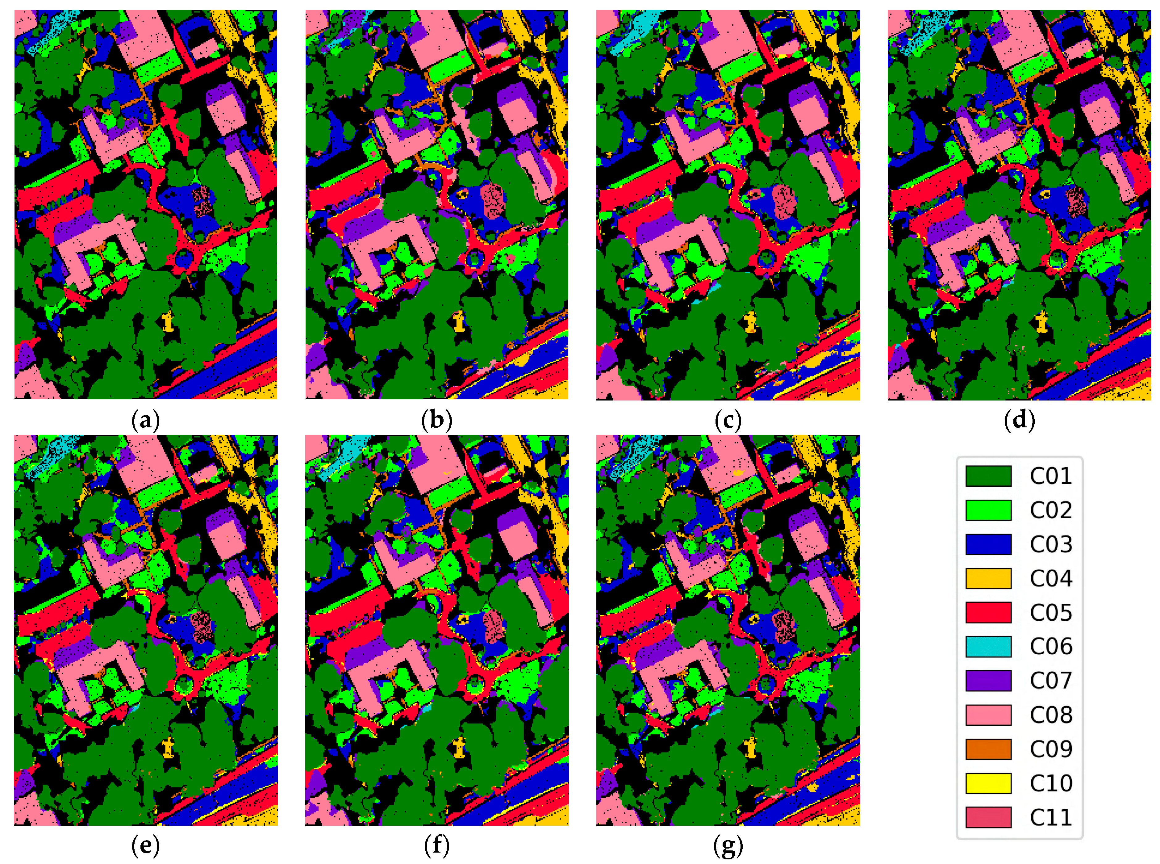
As shown in Table 8, among all five comparative models, Cross-HL achieves the highest overall accuracy. And it shows higher per-class accuracy than H-FANet for Trees, Building Shadow, and Fabric Panel. However, H-FANet still achieves the highest OA, AA, and Kappa values across all models, with an OA of 92.11 ± 0.05% and an AA of 75.47 ± 0.03%. The low AA value was mainly due to the poor performance on two minority categories. The Yellow Curb Strip has only 83 test samples in the dataset. Its spectral signature is highly similar to that of Road and Sidewalk, making it prone to misclassification. All six models achieve accuracy below 30% for this category, indicating that the difficulty is inherent to the data characteristics rather than specific to any single method. Similarly, the Fabric Panel class has only 169 test samples, which is a spatially small target. Its features are easily obscured by the dominant categories within the $11 \times 11$ receptive field. These results suggest that future work should focus on data augmentation strategies or adaptive attention mechanisms designed specifically for minority and spatially compact categories. Figure 14 illustrates the classification results of each model on the Muufl Gulfport dataset.

5.2. Sensitivity Analysis with Different Numbers of Training Samples

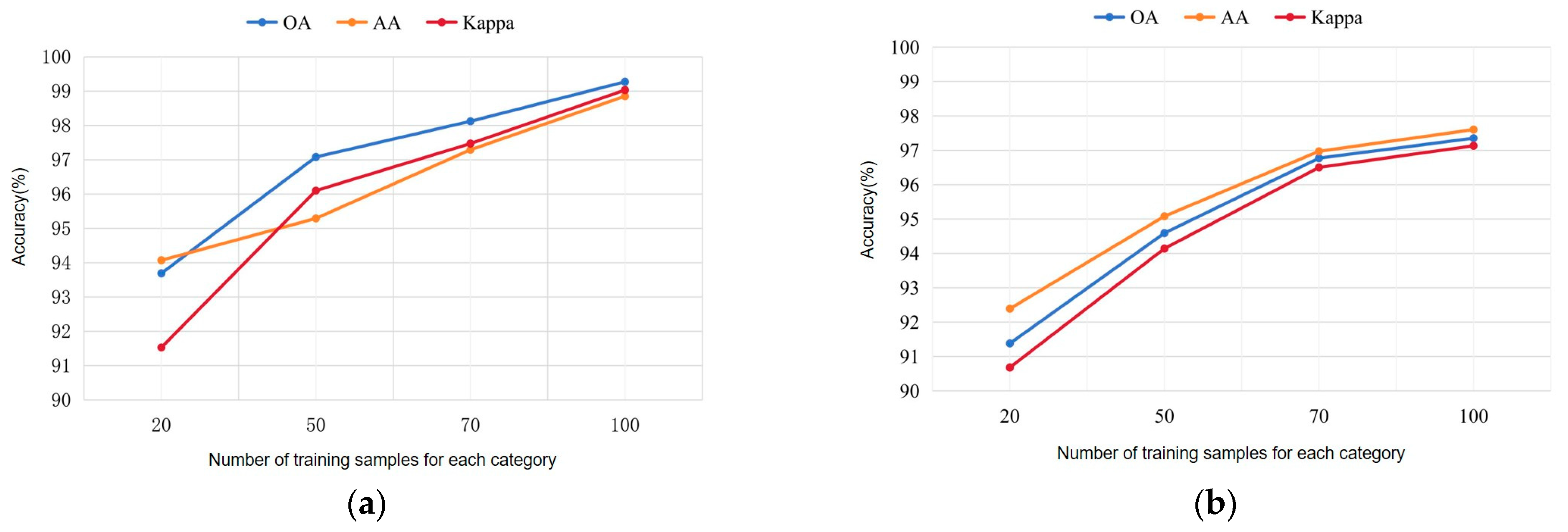
To evaluate the network’s robustness with respect to the size of the training set, this section presents classification performance experiments conducted on the Trento and Houston 2013 datasets using varying numbers of training samples. Specifically, the quantities of training samples per category are set to 20, 50, 70, and 100. As shown in

Table 9. Classification results of different numbers of training samples on the Trento dataset (%).

Number of Training Samples per Category	OA ↑	AA ↑	Kappa ↑
20	93.69	94.07	91.53
50	97.08	95.29	96.10
70	98.12	97.29	97.47
100	99.27	98.85	99.03

↑ indicates that higher values denote better performance.

, for the Trento dataset, even when only 20 training samples per category are used, the model achieves high accuracy, with OA and AA reaching approximately 94%, and a Kappa coefficient of 91.53%. As the quantity of training samples rises to 100 per category, OA exceeds 99%.

Performance of the model on the Houston 2013 dataset is presented in

Table 10. Classification results of different numbers of training samples on the Houston 2013 dataset (%).

Number of Training Samples per Category	OA ↑	AA ↑	Kappa ↑
20	91.38	92.39	90.68
50	94.59	95.08	94.14
70	96.77	96.97	96.50
100	97.35	97.60	97.13

↑ indicates that higher values denote better performance.

. When the number of training samples for each category is limited to 20, the OA has reached a high level of 91.38%. When the number of training samples increased to 100, both OA and AA reached 97%. These results indicate that the proposed H-FANet network can still maintain a high classification effect even in the case of limited training data, which exactly verifies its powerful ability for feature representation and fusion.

Figure 15 clearly illustrates that when the quantity of training samples per category rises, the model achieves better overall performance. This trend is more evident in the two datasets.

5.3. Ablation Experiments on Module Effectiveness

The proposed method is further developed on the basis of the existing three-branch architecture by fully mining diverse feature information in the data. For the two modalities of space and elevation, multi-scale feature enhancement modules (SpaMsE and EleMsE) were specially designed to enhance the perception ability of local structures and scale invariance, so as to compensate for the limited modeling capabilities of the original spatial and elevation branches.

Meanwhile, a hierarchical feature fusion strategy was introduced to achieve compact integration and effective interaction of features. Across the entire network, each multi-scale feature enhancement module and every layer within the feature fusion module play a crucial role in performance improvement. In order to assess the effectiveness of individual components, ablation studies are conducted to compare classification performance with and without each module.

Table 11. Impact of each module on the classification accuracy of the Trento dataset (%).

Evaluation Metrics	SpaMsE (✕)	EleMsE (✕)	SF2A (✕)	DF2C (✕)	H-FANet
OA ↑	98.61	98.69	92.02	94.86	99.27
AA ↑	98.41	97.93	92.24	95.42	98.85
Kappa ↑	98.13	98.25	89.29	93.07	99.03

✕ Indicates that the corresponding module is removed in the ablation setting; ↑ Indicates that higher values denote better performance.

and

Table 12. Impact of each module on the classification accuracy of the Houston 2013 dataset (%).

Evaluation Metrics	SpaMsE (✕)	EleMsE (✕)	SF2A (✕)	DF2C (✕)	H-FANet
OA ↑	95.54	94.52	95.34	94.99	97.35
AA ↑	96.17	95.27	96.13	95.62	97.60
Kappa ↑	95.17	94.07	94.95	94.57	97.13

✕ Indicates that the corresponding module is removed in the ablation setting; ↑ Indicates that higher values denote better performance.

present the impact of individual modules on classification accuracy for the Trento dataset and the Houston 2013 dataset, respectively.

According to the data in Table 11, each feature enhancement module contributes positively to classification accuracy on the Trento dataset. The absence of either the SpaMsE or the EleMsE results in a reduction in OA by less than 1%, indicating that the backbone three-branch extraction alone retains strong baseline performance. The two fusion modules have a considerably larger impact. Removing SF2A causes the most notable performance drop, with OA declining by 7.25%, AA by 6.61%, and Kappa by 9.74%. Removing DF2C also leads to a clear degradation, decreasing OA by 4.41%, AA by 3.43%, and Kappa by 5.96%. These results suggest that the hierarchical fusion strategy is the primary driver of H-FANet’s performance improvement on this dataset, with SF2A contributing more than DF2C.

It can be seen from the data in Table 12 that each feature enhancement module has positively and effectively improved the classification accuracy of the Houston 2013 dataset. Among the two modules, the influence of the EleMsE is more significant. When this module is removed, OA decreases by approximately 3%, AA decreases by approximately 2%, and the Kappa coefficient also drops by approximately 3%.

Combining the experimental results from the two datasets indicates that H-FANet effectively improves the feature modeling ability by introducing the multi-scale enhancement module and the hierarchical fusion mechanism on the basis of retaining the three-branch feature extraction architecture.

Specifically, the multi-scale feature enhancement module enhances local details and optimizes structural perception for the spatial and elevation features in HSI. While greatly strengthening the feature expression ability within the region of interest, it minimizes information loss to a large extent.

We note that the proposed method is designed within a three-branch fusion framework, and its main contribution lies in the multi-scale enhancement and hierarchical fusion strategy rather than single-modality classification. Therefore, single-modality baselines (e.g., HSI-only or LiDAR-only) are not included in the current ablation study. Additionally, the patch size of $11 \times 11$ was selected based on a balance between receptive field coverage and computational cost. Exploring adaptive patch sizes or modality-specific contribution analysis will be considered in future work.

To further evaluate model efficiency, we analyze the computational complexity of H-FANet in terms of the number of parameters and FLOPs. Since the number of input spectral bands differs across the three datasets, the FLOPs may vary slightly, whereas the number of model parameters remains unchanged. Therefore, the reported value is provided as a representative estimate of the computational complexity of H-FANet. As evaluated on the Trento dataset, H-FANet contains approximately 15.7 M parameters and requires 0.64 GFLOPs per input sample.

6. Discussion

The three-branch architecture separates the input into spectral, spatial, and elevation streams. Each stream is allowed to learn its own representation before any cross-modal mixing takes place. Spectral features capture material identity, spatial features carry texture and form, and elevation features encode geometry. Keeping them apart during early extraction avoids the interference that tends to arise when heterogeneous signals are fused too soon. The hierarchical fusion stage then brings them back together, recovering complementary cross-modal relationships in a controlled manner rather than forcing an early merge.

SpaMsE and EleMsE approximate scale invariance through parallel convolutions of different receptive fields followed by hierarchical aggregation. SpaMsE handles two-dimensional texture continuity in HSI, and EleMsE targets sparse elevation gradients in LiDAR. The two modules do not share parameters, which prevents the modeling bias that arises from forcing heterogeneous modalities into a shared representation. Reducing the shallow extraction depth from four blocks to three and compensating with multi-scale enhancement cuts redundant feature capture while keeping the parameter count manageable for the available training samples. The ablation results confirm that this scale diversity contributes meaningfully to feature representation. On the fusion side, H-FANet differs from MAHiDFNet in how cross-modal interaction is staged. MAHiDFNet fuses all three modalities at the shallow level through channel reweighting and concatenation, which risks premature coupling and noise amplification. Its deep stage then integrates high-level features in a serial pixel-wise manner without any residual or grouping mechanism, making it hard to separate shape from material information. H-FANet avoids both problems by splitting fusion into shallow geometric alignment (SF2A) and deep semantic integration (DF2C), as described in Section 3.5 and Section 3.6.

H-FANet further separates shape-level alignment from material-level reasoning. SF2A operates only between the spatial and elevation branches, leaving the spectral path untouched. This is because texture and elevation share common geometric structure and can be cross-corrected at a low semantic level, whereas spectral vectors encoding material composition are better held back until context discrimination is stronger. DF2C then brings all three branches together through group residual aggregation followed by a single linear fusion step. Deferring spectral integration to this deeper stage acts as a late binding strategy that keeps material signatures clean and avoids the noise propagation that early fusion tends to cause. The two-stage residual design in DF2C also creates a shorter gradient path, complementing the shallow alignment done by SF2A. The ablation results bear this out. Removing the shallow fusion module causes a steeper drop than removing the deep fusion module. Early geometric alignment thus turns out to be the more critical of the two stages.

Several limitations should be acknowledged. First, the attention mechanism depends on adequate training samples per category, so rare classes such as Yellow Curb Strip remain prone to misclassification. Second, the fixed $11\times 11$ receptive field limits the delineation of narrow linear targets. Third, patch-based sampling extracts overlapping neighborhoods, which introduces spatial autocorrelation between training and test samples and may inflate accuracy estimates. Fourth, evaluation is restricted to three widely used benchmarks, and the applicability to new geographic regions or different sensor types remains unverified. Fifth, the three-branch design with dual multi-scale modules adds computational overhead (approximately 16 M parameters and 0.64 GFLOPs per sample), which is moderate but non-negligible for resource-constrained settings.

Performance gains of H-FANet vary across datasets and categories. The six categories in the Trento dataset are well separated with compact spatial distributions, and the overall OA exceeds 99%. Terrain variation in the Muufl Gulfport dataset is substantial, and the elevation branch contributes significantly to distinguishing built-up surfaces from natural ground cover. Minority categories show greater accuracy gains from the multi-scale modules than well-sampled categories. Categories with fewer than 200 test samples in the Muufl Gulfport dataset (83 samples in Yellow Curb Strip and 169 samples in Fabric Panel) exhibit greater relative improvements. A comparable pattern is observed in the Houston 2013 dataset, where Water body (225 samples) and Tennis court (328 samples) benefit more than the majority categories. The multi-scale design appears to alleviate data scarcity through convolutional diversity. Extremely rare categories nonetheless require further investigation.

A potential concern is whether comparing a CNN model against Transformer-based alternatives is fair. MAHiDFNet, the direct baseline of H-FANet, is itself a CNN three-branch architecture. And H-FANet improves over it consistently across all three datasets. These gains trace back to the module-level designs rather than to differences in architectural paradigm. That H-FANet also outperforms the Transformer-based methods on the same benchmarks suggests a well-designed multi-scale enhancement scheme with staged hierarchical fusion can hold its own against global self-attention for this task.

7. Conclusions

H-FANet is proposed as a hierarchical fusion attention network for hyperspectral-LiDAR land cover classification. The design combines a three-branch architecture with modality-specific multi-scale enhancement modules for spatial and elevation features. A two-stage fusion strategy performs shallow geometric alignment through SF2A and deep semantic integration through DF2C. Experiments on three benchmark datasets demonstrate the effectiveness of this approach. H-FANet achieves OA of 99.13 ± 0.06% on Trento, 97.43 ± 0.06% on Houston 2013, and 92.11 ± 0.05% on Muufl Gulfport. These results surpass five competing methods (EndNet, MAHiDFNet, MFT, GLT-Net, and Cross-HL) by approximately 1.7–2.2% in OA across the three datasets. The OA remains above 90% even with only 20 training samples per class in the small-sample experiments. Ablation experiments show that removing the fusion modules causes much larger accuracy drops than removing the multi-scale modules, confirming that hierarchical fusion is the main source of improvement. The multi-scale modules still provide meaningful gains for minority categories that lack sufficient training data.

Several limitations remain. The fixed $11\times 11$ patch size may be suboptimal for objects of varying spatial extents. The model requires adequate training samples per category and incurs computational overhead of approximately 16 M parameters and 0.64 GFLOPs per sample. Future work will explore adaptive patch selection and evaluate transferability to new geographic regions and sensor configurations.

References

- Chen, B.; Huang, B.; Xu, B. Multi-source remotely sensed data fusion for improving land cover classification. ISPRS J. Photogramm. Remote Sens. 2017, 124, 27–39. [Google Scholar] [CrossRef] [Scilit]
- Huang, W.; Wu, T.; Zhang, X.; Li, L.; Lv, M.; Jia, Z.; Zhao, X.; Ma, H.; Vivone, G. MCFTNet: Multimodal Cross-Layer Fusion Transformer Network for Hyperspectral and LiDAR Data Classification. IEEE J. Sel. Top. Appl. Earth Obs. Remote Sens. 2025, 18, 12803–12818. [Google Scholar] [CrossRef] [Scilit]
- Gültekin, F.; Koz, A.; Bahmanyar, R.; Azimi, S.M.; Süzen, M.L. Fusing Convolution and Vision Transformer Encoders for Object Height Estimation from Monocular Satellite and Aerial Images. In Proceedings of the 2025 IEEE/CVF International Conference on Computer Vision Workshops (ICCVW), Honolulu, HI, USA, 19–20 October 2025; pp. 3768–3777. [Google Scholar]
- Tang, Y.; Nie, W.; Zhang, Y.; Li, C.; Wei, Z.; Chen, H.; Hu, Y.; Li, W. Rapid identification of Fritillaria spp. using multi-wavebands spectroscopy and multi-source data fusion strategies. J. Appl. Res. Med. Aromat. Plants 2025, 46, 100636. [Google Scholar] [CrossRef] [Scilit]
- Shirmard, H.; Farahbakhsh, E.; Müller, R.D.; Chandra, R. A review of machine learning in processing remote sensing data for mineral exploration. Remote Sens. Environ. 2022, 268, 112750. [Google Scholar] [CrossRef] [Scilit]
- Yuan, J.; Wang, S.; Wu, C.; Xu, Y. Fine-Grained Classification of Urban Functional Zones and Landscape Pattern Analysis Using Hyperspectral Satellite Imagery: A Case Study of Wuhan. IEEE J. Sel. Top. Appl. Earth Obs. Remote Sens. 2022, 15, 3972–3991. [Google Scholar] [CrossRef] [Scilit]
- Ullah, F.; Ullah, I.; Khan, K.; Khan, S.; Amin, F. Advances in deep neural network-based hyperspectral image classification and feature learning with limited samples: A survey. Appl. Intell. 2025, 55, 370. [Google Scholar] [CrossRef] [Scilit]
- Liu, J.; Li, L.; Zhao, X.; Lv, M.; Jia, Z.; Zhang, X.; Vivone, G.; Ma, H. CMNet: Global–Local Feature Fusion CNN-Mamba Network for Remote Sensing Object Detection. Remote Sens. 2026, 18, 591. [Google Scholar] [CrossRef] [Scilit]
- Muzammal, M.; Talat, R.; Sodhro, A.H.; Pirbhulal, S. A multi-sensor data fusion enabled ensemble approach for medical data from body sensor networks. Inf. Fusion 2020, 53, 155–164. [Google Scholar] [CrossRef] [Scilit]
- Hong, D.; Yokoya, N.; Chanussot, J.; Zhu, X.X. CoSpace: Common Subspace Learning From Hyperspectral-Multispectral Correspondences. IEEE Trans. Geosci. Remote Sens. 2019, 57, 4349–4359. [Google Scholar] [CrossRef] [Scilit]
- Liu, X.; Zhu, X.; Li, M.; Wang, L.; Tang, C.; Yin, J.; Shen, D.; Wang, H.; Gao, W. Late Fusion Incomplete Multi-View Clustering. IEEE Trans. Pattern Anal. Mach. Intell. 2019, 41, 2410–2423. [Google Scholar] [CrossRef] [Scilit] [PubMed]
- Bilal, O.; Khan, S.U.R.; Mistry, S.; Deb, N.; Mahmud, M.; Bhuyan, M. Towards Efficient Pruning and Multi-Scale Feature Transformations to Uncover Medical Diseases. In Proceedings of the 2025 International Joint Conference on Neural Networks (IJCNN), Rome, Italy, 30 June–5 July 2025; pp. 1–8. [Google Scholar]
- Lu, D.; Cheng, S.; Wang, L.; Song, S. Multi-scale feature progressive fusion network for remote sensing image change detection. Sci. Rep. 2022, 12, 11968. [Google Scholar] [CrossRef] [Scilit] [PubMed]
- Liu, G.; Song, J.; Chu, Y.; Zhang, L.; Li, P.; Xia, J. Deep Fuzzy Fusion Network for Joint Hyperspectral and LiDAR Data Classification. Remote Sens. 2025, 17, 2923. [Google Scholar] [CrossRef] [Scilit]
- Han, G.; Huang, S.; Zhao, F.; Tang, J. SIAM: A parameter-free, Spatial Intersection Attention Module. Pattern Recognit. 2024, 153, 110509. [Google Scholar] [CrossRef] [Scilit]
- Wu, C.; Tong, L.; Zhou, J.; Xiao, C. Spectral–Spatial Large Kernel Attention Network for Hyperspectral Image Classification. IEEE Trans. Geosci. Remote Sens. 2024, 62, 5508814. [Google Scholar] [CrossRef] [Scilit]
- Wang, X.; Feng, Y.; Song, R.; Mu, Z.; Song, C. Multi-attentive hierarchical dense fusion net for fusion classification of hyperspectral and LiDAR data. Inf. Fusion 2022, 82, 1–18. [Google Scholar] [CrossRef] [Scilit]
- Feng, Y.; Zhu, J.; Song, R.; Wang, X. S2EFT: Spectral-Spatial-Elevation Fusion Transformer for hyperspectral image and LiDAR classification. Knowl.-Based Syst. 2024, 283, 111190. [Google Scholar] [CrossRef] [Scilit]
- Li, H.C.; Wang, W.Y.; Pan, L.; Li, W.; Du, Q.; Tao, R. Robust Capsule Network Based on Maximum Correntropy Criterion for Hyperspectral Image Classification. IEEE J. Sel. Top. Appl. Earth Obs. Remote Sens. 2020, 13, 738–751. [Google Scholar] [CrossRef] [Scilit]
- Roy, S.K.; Deria, A.; Hong, D.; Rasti, B.; Plaza, A.; Chanussot, J. Multimodal Fusion Transformer for Remote Sensing Image Classification. IEEE Trans. Geosci. Remote Sens. 2023, 61, 5515620. [Google Scholar] [CrossRef] [Scilit]
- Ozkan, S.; Kaya, B.; Akar, G.B. EndNet: Sparse AutoEncoder Network for Endmember Extraction and Hyperspectral Unmixing. IEEE Trans. Geosci. Remote Sens. 2019, 57, 482–496. [Google Scholar] [CrossRef] [Scilit]
- Li, X.; Song, C.; Zhang, C.; Lan, J.; Zhu, H.; Wang, W.; Sun, X. Hybrid Vision Transformer and Convolutional Neural Network for Super-Resolution Image Quality Assessment. In Proceedings of the 2025 IEEE/CVF International Conference on Computer Vision Workshops (ICCVW), Honolulu, HI, USA, 19–20 October 2025; pp. 3354–3361. [Google Scholar]
- Xu, Z.; Jiang, W.; Geng, J. Dual-Branch Dynamic Modulation Network for Hyperspectral and LiDAR Data Classification. IEEE Trans. Geosci. Remote Sens. 2023, 61, 5514813. [Google Scholar] [CrossRef] [Scilit]
- Chen, X.; Ma, M.; Li, Y.; Mei, S.; Han, Z.; Zhao, J.; Cheng, W. Hierarchical Feature Fusion of Transformer with Patch Dilating for Remote Sensing Scene Classification. IEEE Trans. Geosci. Remote Sens. 2023, 61, 4410516. [Google Scholar] [CrossRef] [Scilit]
- Ding, K.; Lu, T.; Fu, W.; Li, S.; Ma, F. Global–Local Transformer Network for HSI and LiDAR Data Joint Classification. IEEE Trans. Geosci. Remote Sens. 2022, 60, 5541213. [Google Scholar] [CrossRef] [Scilit]
- Li, Z.; Liu, R.; Sun, L.; Zheng, Y. Multi-Feature Cross Attention-Induced Transformer Network for Hyperspectral and LiDAR Data Classification. Remote Sens. 2024, 16, 2775. [Google Scholar] [CrossRef] [Scilit]
- Wang, M.; Fang, S.; Li, Y.; Zhang, X.; Li, Z. A hybrid CNN-transformer network with difference enhancement and frequency fusion for remote sensing image change detection. Appl. Intell. 2025, 56, 8. [Google Scholar] [CrossRef] [Scilit]
- Jiang, Y.; Liu, S.; Wang, H. Diffusion-based remote sensing image fusion for classification. Appl. Intell. 2024, 55, 247. [Google Scholar] [CrossRef] [Scilit]
- Su, Z.; Chen, J.; Pang, L.; Ngo, C.W.; Jiang, Y.G. Adaptive Split-Fusion Transformer. In Proceedings of the 2023 IEEE International Conference on Multimedia and Expo (ICME), Brisbane, Australia, 10–14 July 2023; pp. 1169–1174. [Google Scholar]
- Wang, Q.; Wu, B.; Zhu, P.; Li, P.; Zuo, W.; Hu, Q. ECA-Net: Efficient Channel Attention for Deep Convolutional Neural Networks. In Proceedings of the 2020 IEEE/CVF Conference on Computer Vision and Pattern Recognition (CVPR), Seattle, WA, USA, 14–19 June 2020; pp. 11531–11539. [Google Scholar]
- Wang, X.; Zhu, J.; Feng, Y.; Wang, L. MS2CANet: Multiscale Spatial–Spectral Cross-Modal Attention Network for Hyperspectral Image and LiDAR Classification. IEEE Geosci. Remote Sens. Lett. 2024, 21, 5501505. [Google Scholar] [CrossRef] [Scilit]
- Zhang, M.; Li, W.; Zhang, Y.; Tao, R.; Du, Q. Hyperspectral and LiDAR Data Classification Based on Structural Optimization Transmission. IEEE Trans. Cybern. 2023, 53, 3153–3164. [Google Scholar] [CrossRef] [Scilit] [PubMed]
- Shang, Y.; Cheng, B.; Zhang, Z.; Wang, Q.; Jin, P.; Huang, L.; Liu, C.; Huang, L.; Ding, X.; Shen, T.; et al. Artificial Intelligence for Remote Sensing: Progress, Challenges, and Perspectives. IEEE J. Sel. Top. Appl. Earth Obs. Remote Sens. 2026, 19, 6840–6874. [Google Scholar] [CrossRef] [Scilit]
Figure 1.
H-FANet framework.
Figure 2.
Spectral and spatial branches of HSI input.
Figure 3.
Elevation branch of the LiDAR input.
Figure 4.
SpeA module structure.
Figure 5.
SpaMsE module structure.
Figure 6.
EleMsE module structure.
Figure 7.
SF2A module structure.
Figure 8.
DF2C module structure.
Figure 9.
Visualization of the Trento dataset.
Figure 10.
Visualization of the Houston 2013 dataset.
Figure 11.
Visualization of the Muufl Gulfport dataset.
Figure 12.
Classification maps of different models on the Trento dataset. (a) Ground truth map; (b) EndNet; (c) MAHiDFNet; (d) MFT; (e) GLT-Net; (f) Cross-HL; (g) H-FANet.
Figure 13.
Classification maps of different models on the Houston 2013 dataset. (a) Ground truth map; (b) EndNet; (c) MAHiDFNet; (d) MFT; (e) GLT-Net; (f) Cross-HL; (g) H-FANet.
Figure 14.
Classification maps of different models on the Muufl Gulfport dataset. (a) Ground truth map; (b) EndNet; (c) MAHiDFNet; (d) MFT; (e) GLT-Net; (f) Cross-HL; (g) H-FANet.
Figure 15.
Performance comparison of H-FANet under different numbers of training samples. (a) Trento dataset; (b) Houston 2013 dataset.