Static–Dynamic Coupling of Landscape Ecological Risk and Ecosystem Service Value in an Arid Urban Agglomeration: Evidence from the Northern Slope of the Tianshan Mountains

Abstract

Land-use change in arid urban agglomerations reshapes landscape ecological risk (LER) and ecosystem service value (ESV), yet few studies jointly diagnose their current coupling state, temporal trajectory, and future scenario response. Focusing on the urban agglomeration on the northern slope of the Tianshan Mountains, we integrated land-use data for 2000, 2010, and 2020 with LER assessment, ESV estimation, static–dynamic coupling zoning, and intPLUS-based 2030 scenario simulation. From 2000 to 2020, cropland and construction land expanded by 46.43% and 107.84%, whereas forest and water bodies declined by 49.76% and 47.64%. LER was dominated by low- and medium-low-risk classes, although medium-high-risk areas expanded locally. Total ESV declined from 512.16 to 429.97 billion CNY, with continued contraction of medium-high- and high-ESV zones. In 2020, potential enhancement zones (PEZs) dominated the integrated management pattern, accounting for 43.64% of the study area. By 2030, static zoning changed only slightly, whereas dynamic and integrated zoning showed clear scenario sensitivity: PEZs accounted for 40.55% under the natural development scenario, while priority governance zones reached 49.06% and 49.26% under economic development and ecological protection scenarios. By treating LER as risk pressure and ESV as service-supply capacity, this framework links static risk–service matching, dynamic trajectory diagnosis, and future scenario response, thereby supporting ecological zoning in arid urban agglomerations.

1. Introduction

Land-use/cover change is a major driver of regional ecological security and ecosystem service provision. Urban expansion, agricultural development, and infrastructure construction alter not only land-use composition but also landscape structure, ecological processes, and service functions. These effects are particularly acute in arid urban agglomerations, where limited water and land resources, oasis agriculture, urban growth, and ecological protection demands overlap spatially. Such interactions can intensify mismatches between landscape ecological risk and ecosystem service value. Land-use transitions and urban expansion can directly affect biodiversity and carbon stocks, especially where built-up land expands into ecological spaces [1,2]. Ecological conservation and natural-capital investment have improved ecosystem services in parts of China, but risk–service conflicts may remain pronounced in rapidly developing regions [3].

Landscape ecological risk (LER) and ecosystem service value (ESV) are complementary but non-substitutable indicators of ecological security. LER represents risk pressure generated by landscape disturbance, ecological vulnerability, and potential ecological loss, and is commonly used to diagnose ecological risk under land-use change [4,5]. ESV represents ecosystem service-supply capacity by translating land-use or ecosystem types into monetary values of provisioning, regulating, supporting, and cultural services [6,7]. Spatially explicit ecosystem-service mapping also provides a basis for comparing service supply across heterogeneous landscapes [8]. Therefore, LER–ESV coupling should not be interpreted as a simple negative correspondence between risk and value. High-risk areas do not necessarily have low ESV, and high-ESV areas may also show high LER when key ecological patches, such as water bodies, forests, and grasslands, are fragmented or disturbed.

Despite these advances, three gaps remain. First, separate LER or ESV assessments cannot reveal whether ecological risk pressure and service-supply capacity are spatially matched or mismatched. Second, recent LER–ESV and LER–ES studies have improved ecological security assessment, but most still emphasize coupling relationships, correlations, or static classifications. Wang et al. [9] incorporated LER into ESV assessment, while Li et al. [10] used LER–ESV relationships for ecological zoning and simulation. At the urban-agglomeration scale, Xiong et al. [11] integrated LER and ESV into ecological security pattern identification, and Liu and Tang [12] further linked LER with multiple ecosystem services for management zoning. These studies provide important foundations, but they do not fully integrate current state, historical trajectory, and future scenario response.

The urban agglomeration on the northern slope of the Tianshan Mountains (UANSTM) provides a representative setting for addressing these gaps. Located in the arid region of northwestern China, the UANSTM has a typical mountain–oasis–desert landscape and is one of the most concentrated areas of population, industry, and urban activity in Xinjiang. Previous studies have examined urban expansion and its eco-environmental effects in this region [13], changes in ecological environment quality [14,15], and the relationships among ecological risk, land-use transformation, and ecosystem services [16,17]. However, an integrated assessment of the static state, dynamic trajectory, and future scenario response of LER–ESV remains limited.

To address these gaps, we integrated land-use data from 2000, 2010, and 2020 with LER assessment, ESV accounting, static–dynamic coupling zoning, and intPLUS-based multi-scenario simulation to diagnose LER–ESV coupling patterns and their 2030 scenario responses in the UANSTM. Specifically, this study aims to (1) characterize land-use change and the spatiotemporal evolution of LER and ESV from 2000 to 2020; (2) construct a static–dynamic zoning framework that links risk–service matching states with historical trajectories; and (3) update LER–ESV zoning under economic development, natural development, and ecological protection scenarios to reveal future scenario responses of integrated management zones. By linking historical change, coupling state, dynamic trajectory, and future scenario response, this study provides a remote-sensing-based framework for ecological risk identification, ecosystem service maintenance, and zoning management in arid urban agglomerations.

2. Materials and Methods

2.1. Study Area

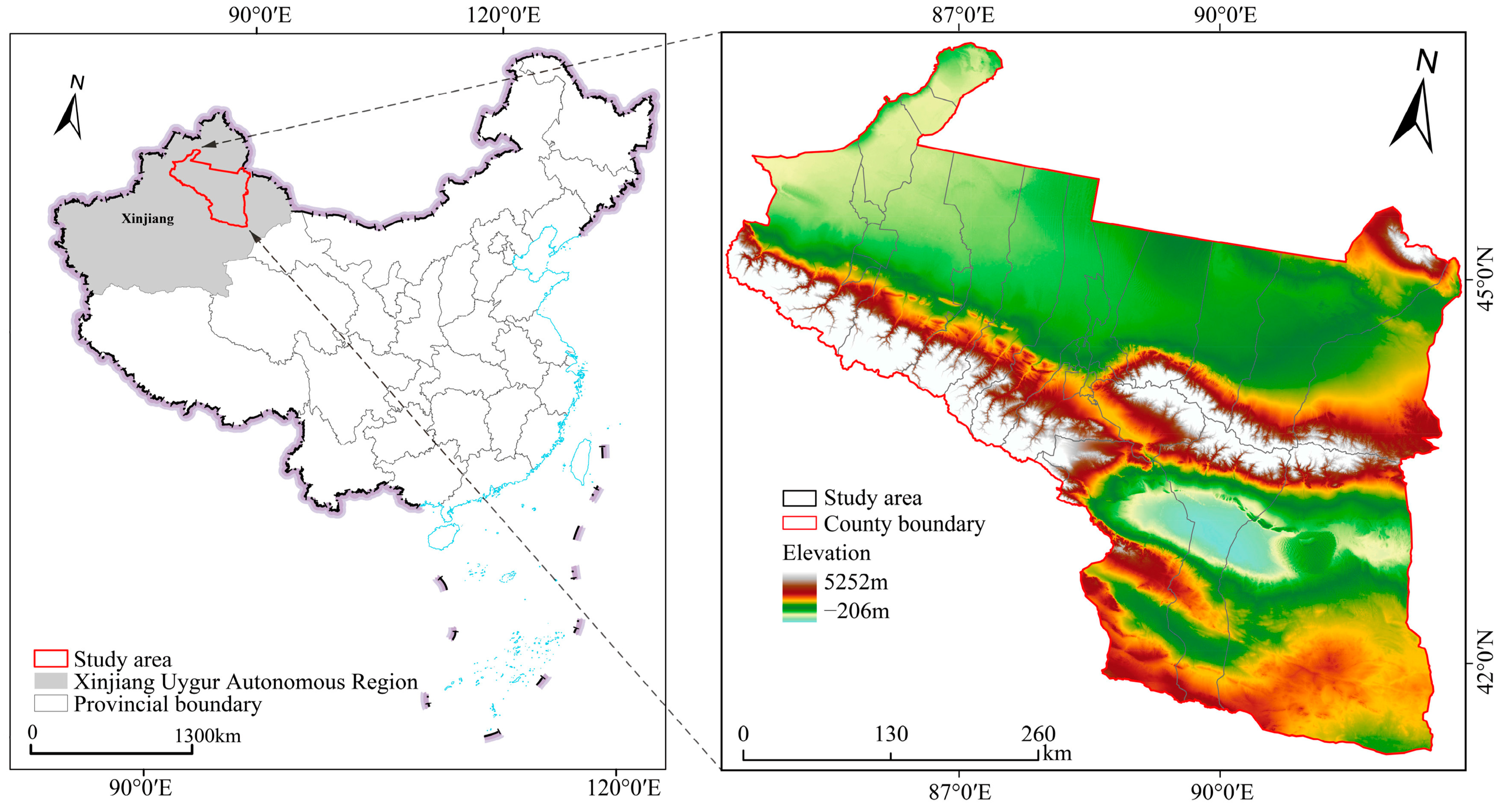
The urban agglomeration on the northern slope of the Tianshan Mountains (UANSTM) is located in northern Xinjiang, China (82°30′–91°30′ E, 39°40′–45°30′ N), between the northern foothills of the Tianshan Mountains and the southern margin of the Junggar Basin. The study area covers approximately 215,400 km² (Figure 1) and includes Urumqi, Changji Hui Autonomous Prefecture, Shihezi, Karamay, and surrounding oasis cities and piedmont plains. It is one of the most concentrated areas of population, industry, and urban activity in Xinjiang.

The UANSTM has a typical arid mountain–oasis–desert landscape. The southern Tianshan Mountains function as important water-conservation and ecological barrier zones. The central piedmont oasis belt contains most cropland, urban land, and transport corridors, and is the most active area of land-use change. The northern and peripheral areas are dominated by desert, Gobi landscapes, and sparse vegetation. The region is therefore both a key space for economic development and urbanization in Xinjiang and a critical area for maintaining ecological security in arid environments, making it suitable for examining LER-ESV coupling and future scenario responses under land-use change.

2.2. Data Sources and Preprocessing

Multi-source spatial and statistical data were used to support land-use change analysis, LER assessment, ESV estimation, and 2030 multi-scenario simulation. Land-use data for 2000, 2010, and 2020, with a spatial resolution of 30 m, were reclassified into six categories: cropland, forest, grassland, water bodies, construction land, and unused land. These data provided the basis for historical land-use analysis, LER and ESV calculation, and intPLUS model calibration.

Physical geographical, socio-economic, and accessibility variables were used as driving factors for land-use simulation. Physical geographical variables included DEM, slope, aspect, annual mean temperature, annual precipitation, sunshine duration, soil type, grazing intensity, soil erosion, and ecological environment-related data. Socio-economic variables included population density, GDP density, and human footprint. Accessibility variables included distances to roads, highways, water bodies, government seats, and points of interest (POIs). Statistical data from the Xinjiang Statistical Yearbook and the National Compilation of Agricultural Product Cost and Revenue Data were used to support ESV coefficient correction and scenario parameter setting. The year, spatial resolution, and dataset provider or source institution of each dataset are listed in

Table 1. Data used in this study and their details.

Data Type	Data Name	Year(s)	Spatial Resolution	Source
Land use	Land use (LUCC)	2000, 2010, 2020	30 m	Resource and Environment Science and Data Center (RESDC)
Physical geography	Annual average temperature	2020	1 km	RESDC
Physical geography	Annual average precipitation	2020	1 km	RESDC
Physical geography	Sunshine duration	2020	1 km	National Tibetan Plateau Data Center (TPDC)
Physical geography	Soil type	2020	1 km	RESDC
Physical geography	DEM	2020	30 m	Geospatial Data Cloud
Physical geography	Slope	2020	30 m	Calculated from DEM
Physical geography	Aspect	2020	30 m	Calculated from DEM
Physical geography	Grazing intensity	2020	1 km	Global Resource Data Cloud
Physical geography	Soil erosion	2020	1 km	Global Resource Data Cloud
Physical geography	China’s ecological issues data	2020	90 m	Research Center for Eco-Environmental Sciences, Chinese Academy of Sciences
Socio-economic	Population density	2020	1 km	RESDC
Socio-economic	GDP density	2020	1 km	RESDC
Socio-economic	Human footprint	2020	1 km	Global Human Footprint dataset/figshare repository
Socio-economic	Other statistical data	2000, 2010	—	Statistical Yearbook of the Xinjiang Uygur Autonomous Region; National Compilation of Agricultural Product Cost and Revenue Data
Accessibility	Distance to roads	2020	—	OpenStreetMap (OSM)
Accessibility	Distance to highways	2020	—	OSM
Accessibility	Distance to water	2020	—	OSM
Accessibility	Distance to government	2020	—	National Bureau of Statistics
Accessibility	Distance to POI	2020	—	OSM

Note: “—” indicates that spatial resolution is not applicable to the corresponding vector or statistical data. The listed resolutions refer to the original datasets; all raster layers were harmonized to a 30 m × 30 m grid before spatial analysis. Full access links and dataset DOIs are provided in the Data availability statement.

.

All raster datasets were preprocessed in ArcGIS 10.8 (Esri, Redlands, CA, USA) to ensure cross-source spatial consistency. They were projected to the Asia_North_Albers_Equal_Area_Conic coordinate system, clipped to the study boundary, resampled, and aligned to a 30 m × 30 m raster grid. Categorical variables, such as land-use and soil type, were resampled using the nearest-neighbor method, whereas continuous variables, including DEM, climate, population density, GDP density, grazing intensity, soil erosion, and human footprint, were resampled using bilinear interpolation. Missing raster values were filled by linear interpolation where necessary. Accessibility variables were generated as Euclidean-distance rasters from roads, highways, water bodies, POIs, and government locations. The harmonized 30 m raster layers were used for land-use transition analysis and intPLUS simulation, and were further aggregated within 5 km × 5 km evaluation grids for LER, ESV, and LER–ESV zoning.

2.3. Analytical Framework

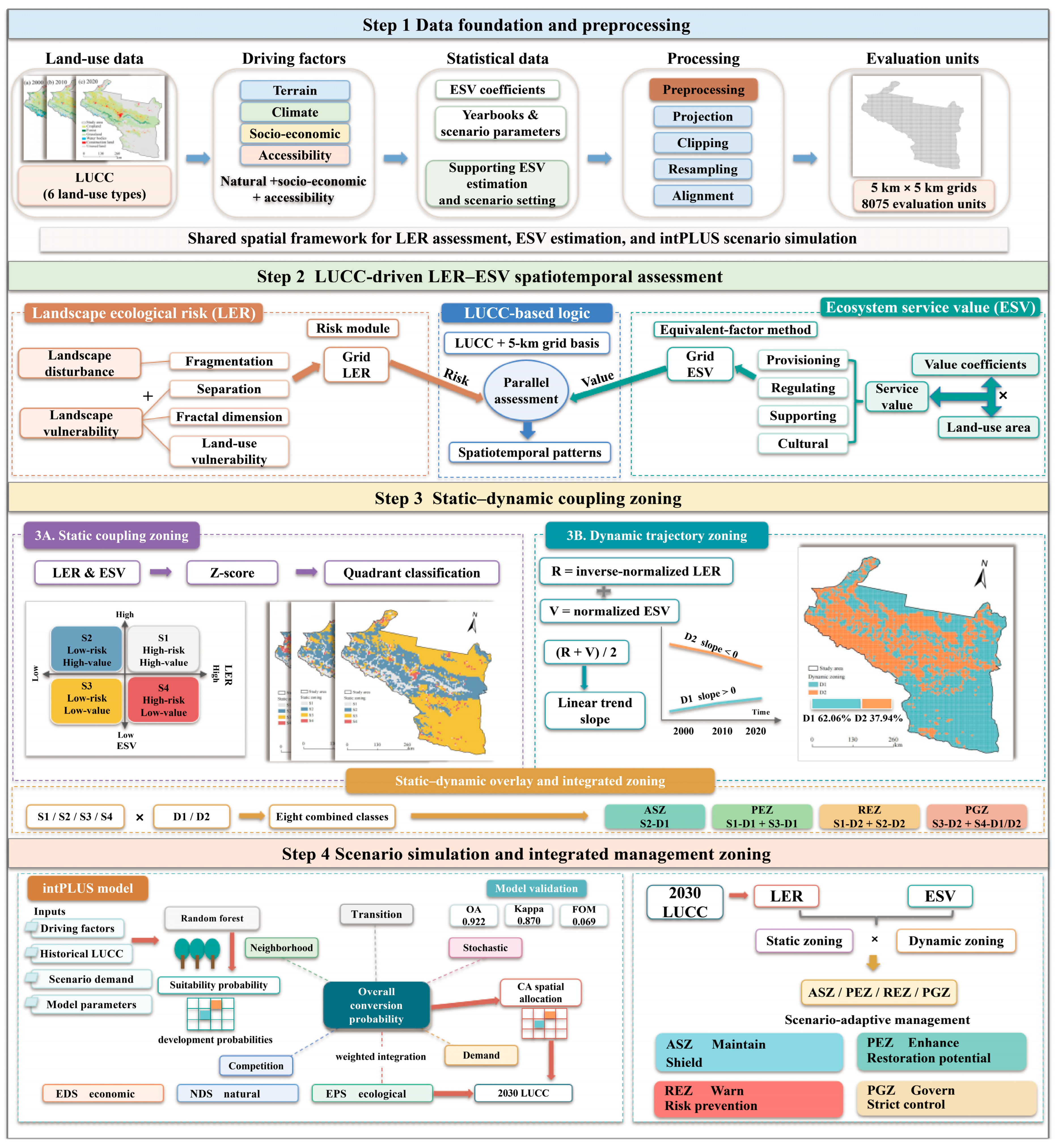
This study developed a workflow linking land-use change detection, LER and ESV assessment, static–dynamic coupling zoning, and 2030 scenario simulation and zoning update (Figure 2). The workflow was designed not as a direct overlay of LER and ESV maps, but as a sequential diagnosis of static risk–service state, historical trajectory, and future scenario response. First, land-use data from 2000, 2010, and 2020 were used to quantify changes in area, dynamic degree, and transition pathways, providing the land-use basis for LER and ESV assessment.

Second, LER and ESV were calculated at the 5 km × 5 km grid-cell scale to characterize their spatiotemporal evolution from 2000 to 2020. Static quadrant zoning was then constructed using standardized LER and ESV values, and dynamic zoning was identified from the trajectory of the comprehensive state. The static and dynamic zones were overlaid and aggregated into four integrated management zones: ASZ, PEZ, REZ, and PGZ.

Finally, the intPLUS model was used to simulate land-use patterns in 2030 under the economic development scenario (EDS), natural development scenario (NDS), and ecological protection scenario (EPS). LER, ESV, and integrated management zones were then updated based on the simulated land-use patterns. Differences among scenarios were compared to evaluate the potential effects of alternative development pathways on the LER-ESV coupling pattern.

2.4. Land-Use Change Analysis

Following land-use dynamic degree and land-use transfer matrix approaches [18], we calculated the area and proportion of cropland, forest, grassland, water bodies, construction land, and unused land, and then quantified the dynamic degree of each land-use type:

$$K_i={\displaystyle \frac{U_{i,2}-U_{i,1}}{U_{i,1}}}\times {\displaystyle \frac{1}{T}}\times 100\%$$

(1)

where $K_i$ is the dynamic degree of land-use type $i$; $U_{i,1}$ and $U_{i,2}$ are the areas of land-use type $i$ at the beginning and end of the study period, respectively; and $T$ is the length of the study period. A land-use transition matrix was further constructed as

$$S=\left[\begin{array}{cccc}{S}_{11}& S_{12}& \dots & S_{1n}\\ S_{21}& S_{22}& \dots & S_{2n}\\ ⋮& ⋮& \ddots & ⋮\\ S_{n1}& S_{n2}& \dots & S_{nn}\end{array}\right]$$

(2)

where $S_{\mathit{ij}}$ is the area converted from land-use type $i$ in the initial year to land-use type $j$ in the final year, and $n$ is the number of land-use types. Rows represent initial land-use types, and columns represent final land-use types.

2.5. Ecosystem Service Value Assessment

ESV was estimated using the unit-area value coefficient method, which has been widely applied in ecosystem service valuation and China-specific ESV accounting [6,7]. Based on the land-use classification and value coefficients of the study area, ESV was calculated for cropland, forest, grassland, water bodies, and unused land, while construction land was assigned a value of zero. Unit-area value coefficients for each land-use type and ecosystem service function are listed in

Table 2. Ecosystem service value coefficient per unit area in the UANSTM (CNY/hm²).

Main Type	Minor Type	Value per Unit-Area Coefficient for Each Land-Use Type (RMB/hm2)
		Cropland	Forest	Grassland	Water Bodies	Unused Land
Supply service	Food production	5277.26	1114.35	764.13	1910.32	23.88
	Raw material production	1170.07	2563.01	1122.31	549.22	71.64
	Water supply	−6232.42	1321.31	620.85	24,953.56	47.76
Regulatory service	Gas regulation	4250.46	8405.41	3940.04	2268.51	310.43
	Climate regulation	2220.75	25,152.55	10,411.25	6757.76	238.79
	Environmental remediation	644.73	7482.09	3438.58	13,634.91	979.04
	Hydrological regulation	7139.82	18,195.80	7617.40	261,164.69	573.10
Support service	Soil conservation	2483.42	10,236.13	4799.68	2220.75	358.19
	Maintaining nutrient cycling	740.25	780.05	382.06	167.15	23.88
	Biodiversity Conservation	811.89	9328.73	4369.86	6113.03	334.31
Cultural service	Aesthetic landscape	358.19	4091.27	1934.20	4728.04	143.27

. Total ESV was calculated as

$${\mathit{ESV}}_t={\displaystyle {\sum }_{i=1}^n}{A}_{i,t}\times {\mathit{VC}}_i$$

(3)

where ${\mathit{ESV}}_t$ is the total ecosystem service value in year $t$; $A_{i,t}$ is the area of land-use type $i$ in year $t$; ${\mathit{VC}}_i$ is the unit-area ecosystem service value coefficient of land-use type $i$; and $\mathrm{n}$ is the number of land-use types included in the ESV calculation. The value of each ecosystem service function was calculated as

$${\mathit{ESV}}_{f,t}={\displaystyle {\sum }_{i=1}^n}{A}_{i,t}\times {\mathit{VC}}_{f,i}$$

(4)

where ${\mathit{ESV}}_{f,t}$ is the value of ecosystem service function $f$ in year $t$; $A_{i,t}$ is the area of land-use type $i$ in year $t$; ${\mathit{VC}}_{f,i}$ is the unit-area value coefficient of service function $f$ for land-use type $i$; and $n$ is the number of land-use types included in the calculation. To support grid-scale LER-ESV coupling zoning, ESV was also calculated for each evaluation unit:

$${\mathit{ESV}}_{k,t}={\displaystyle {\sum }_{i=1}^n}{A}_{k,i,t}\times {\mathit{VC}}_i$$

(5)

where ${\mathit{ESV}}_{k,t}$ is the ESV of evaluation unit $k$ in year $t$ and $A_{k,i,t}$ is the area of land-use type $i$ within evaluation unit $k$ in year $t$. ${\mathit{VC}}_i$ is the unit-area ESV coefficient of land-use type $i$; and n is the number of land-use types included in the calculation.

2.6. Landscape Ecological Risk Assessment

LER was calculated using a landscape disturbance–vulnerability–loss framework commonly applied in land-use-based landscape ecological risk assessment [4,19]. The study area was divided into 8075 regular grid cells of 5 km × 5 km, which served as the basic evaluation units. The LER of evaluation unit $k$ was calculated as

$${\mathit{LER}}_k={\displaystyle {\sum }_{i=1}^n}{\displaystyle \frac{A_{k,i}}{A_k}}\times R_i$$

(6)

where ${\mathit{LER}}_k$ is the landscape ecological risk index of evaluation unit $k$; $A_{k,i}$ is the area of land-use type $i$ within unit $k$; $A_k$ is the total area of unit $k$; $R_i$ is the landscape loss index of land-use type $i$; and $n$ is the number of land-use types. The landscape loss index was defined as

$$R_i=E_i\times V_i$$

(7)

where $R_i$ is the landscape loss index of land-use type $i$; $E_i$ is the landscape disturbance index; and $V_i$ is the landscape vulnerability index of land-use type $i$. The disturbance index was calculated from landscape fragmentation, separation, and fractal dimension:

$$E_i={\mathit{aC}}_i+{\mathit{bN}}_i+{\mathit{cF}}_i$$

(8)

where $C_i$, $N_i$, and $F_i$ are the fragmentation, separation, and fractal dimension indices of land-use type $i$, respectively, and $a$, $b$, and $c$ were set to 0.5, 0.3, and 0.2, respectively. The three landscape metrics were calculated as

$$C_i={\displaystyle \frac{n_i}{A_i}}$$

(9)

$$N_i={\displaystyle \frac{A}{2A_i}}\times \sqrt{{\displaystyle \frac{n_i}{A}}}$$

(10)

$$F_i={\displaystyle \frac{2\mathrm{l}\mathrm{n}\left(P_i/4\right)}{\mathrm{l}\mathrm{n}{A}_i}}$$

(11)

where $n_i$ is the number of patches of land-use type $i$; $A_i$, and $P_i$ are the total area and total perimeter of patches of land-use type $i$, respectively; and $A$ is the total landscape area within the calculation unit. The initial vulnerability scores for unused land, water bodies, cropland, grassland, forest, and construction land were set to 6, 5, 4, 3, 2, and 1, respectively, and then normalized. In the order of cropland, forest, grassland, water bodies, construction land, and unused land, the normalized vulnerability values were 0.190, 0.095, 0.143, 0.238, 0.048, and 0.286. A higher ${\mathit{LER}}_k$ value indicates higher landscape ecological risk.

2.7. Static–Dynamic Zoning Framework for LER–ESV Coupling

To diagnose the spatial match or mismatch between ecological risk pressure and service-supply capacity, a static–dynamic LER–ESV zoning framework was developed. Static zoning captures the LER–ESV combination in a given year, whereas dynamic zoning evaluates whether the integrated risk–service condition improves or degrades over time. First, LER and ESV values of evaluation units in the same year were standardized using the Z-score transformation:

$${\mathit{ZLER}}_{k,t}={\displaystyle \frac{{\mathit{LER}}_{k,t}-{\overline{LER}}_t}{S_{LER,t}}}$$

(12)

$${\mathit{ZESV}}_{k,t}={\displaystyle \frac{{\mathit{ESV}}_{k,t}-{\overline{ESV}}_t}{S_{ESV,t}}}$$

(13)

where ${\mathit{ZLER}}_{k,t}$ and ${\mathit{ZESV}}_{k,t}$ are the standardized LER and ESV values of evaluation unit $k$ in year $t$, respectively; ${\overline{\mathit{LER}}}_t$ and ${\overline{\mathit{ESV}}}_t$ are the annual mean values across all evaluation units; and $S_{\mathit{LER},t}$ and $S_{\mathit{ESV},t}$ are the corresponding annual standard deviations. Static quadrant zoning was used to diagnose the current risk–service state of each evaluation unit. S1 denotes high-risk–high-value zones, where high service-supply capacity coexists with elevated risk pressure; S2 denotes low-risk–high-value zones, indicating a favorable risk–service match; S3 denotes low-risk–low-value zones, indicating limited service-supply capacity under relatively low risk pressure; and S4 denotes high-risk–low-value zones, indicating an unfavorable mismatch with high risk pressure and weak service supply.

Second, to identify the comprehensive state trajectory from 2000 to 2020, LER was treated as a negative indicator and ESV as a positive indicator for min-max normalization:

$$R_{k,t}={\displaystyle \frac{{\mathit{LER}}_{max,t}-{\mathit{LER}}_{k,t}}{{\mathit{LER}}_{max,t}-{\mathit{LER}}_{min,t}}}$$

(14)

$$V_{k,t}={\displaystyle \frac{{\mathit{ESV}}_{k,t}-{\mathit{ESV}}_{min,t}}{{\mathit{ESV}}_{max,t}-{\mathit{ESV}}_{min,t}}}$$

(15)

The comprehensive state value was calculated as

$${\mathit{CS}}_{k,t}={\displaystyle \frac{R_{k,t}+V_{k,t}}{2}}$$

(16)

where $R_{k,t}$ is the inverse-normalized risk state of evaluation unit $k$ in year $t$, with larger values indicating lower ecological risk; $V_{k,t}$ is the normalized service-value state of evaluation unit $k$ in year $t$, with larger values indicating higher ESV; ${\mathit{LER}}_{max,t}$ and ${\mathit{LER}}_{min,t}$ are the maximum and minimum LER values across all evaluation units in year $t$; ${\mathit{ESV}}_{max,t}$ and ${\mathit{ESV}}_{min,t}$ are the corresponding maximum and minimum ESVs; and ${\mathit{CS}}_{k,t}$ is the comprehensive state value of evaluation unit $k$ in year $t$. A larger ${\mathit{CS}}_{k,t}$ indicates lower ecological risk and higher ecosystem service value. The trend of ${\mathit{CS}}_{k,t}$ was quantified using the linear regression slope:

$${Slope}_k={\displaystyle \frac{N{\sum }_{r=1}^N{x}_r{CS}_{k,r}-\left({\sum }_{r=1}^N{x}_r\right)\left({\sum }_{r=1}^N{CS}_{k,r}\right)}{N{\sum }_{r=1}^N{x_r}^2-{\left({\sum }_{r=1}^N{x}_r\right)}^2}}$$

(17)

where ${Slope}_k$ is the linear trend slope of the comprehensive state of evaluation unit $k$; $r$ is the temporal order of observations; $x_r$ is the year corresponding to the rth observation; ${CS}_{k,r}$ is the comprehensive state value of evaluation unit $k$ in year $x_r$; and $N$ is the number of time points. Dynamic zoning was used to diagnose the trajectory of the comprehensive state. Units with ${Slope}_k$ > 0 were classified as D1, indicating improvement in the combined low-risk and high-service state, whereas units with ${Slope}_k$ < 0 were classified as D2, indicating degradation. Therefore, D1/D2 reflect whether the comprehensive LER–ESV state improved or deteriorated during 2000–2020.

The static and dynamic zones were then overlaid to identify management priorities based on both state and trajectory. ASZ corresponds to S2-D1, representing low-risk–high-value areas with continued improvement. PEZ includes S1-D1 and S3-D1, representing areas with improvement potential but different management needs. REZ includes S1-D2 and S2-D2, representing high-value or favorable-state areas showing negative trajectories and requiring early warning. PGZ includes S3-D2, S4-D1, and S4-D2, representing low-value or high-risk mismatch areas requiring priority governance.

2.8. intPLUS-Based Scenario Simulation and 2030 Zoning Update

The intPLUS model, developed from the PLUS modeling framework and available at https://github.com/HPSCIL/intPLUS (accessed on 10 July 2026), was used to simulate land-use patterns in 2030 and to update LER, ESV, and integrated management zones [20]. The model learns land-use suitability probabilities from driving factors using a random forest algorithm and estimates pixel-level conversion potential by combining suitability probability, neighborhood effects, stochastic disturbance, inter-class suppression, and quantity constraints:

$${OP}_{p,i}^t=P_{p,i}\times {\Omega }_{p,i}^t\times R_{p,i}^t\times (1-I_{p,i}^t)\times D_i^t$$

(18)

where ${OP}_{p,i}^t$ is the total conversion potential of pixel p to land-use type $i$ at time $t$; $P_{p,i}$ is the suitability probability of pixel p for land-use type i; ${\Omega }_{p,i}^t$ is the neighborhood effect; $R_{p,i}^t$ is the stochastic disturbance term; $I_{p,i}^t$ is the inter-class inhibition term; and $D_i^t$ is the quantity-driven coefficient for land-use type i. The weighted conversion potential was calculated as

$${TP}_{p,i}^t=P_{p,i}^{\alpha }\times {\left({\Omega }_{p,i}^t\right)}^{\beta }\times {\left(R_{p,i}^t\right)}^{\gamma }\times {(1-I_{p,i}^t)}^{\lambda }\times {\left(D_i^t\right)}^{\delta }$$

(19)

where ${TP}_{p,i}^t$ is the weighted total conversion potential of pixel p to land-use type i at time t; $P_{p,i}$, ${\Omega }_{p,i}^t$, $R_{p,i}^t$, $I_{p,i}^t$, and $D_i^t$ represent suitability probability, neighborhood effect, stochastic disturbance, inter-class inhibition, and quantity constraint, respectively; and $\alpha$, $\beta$, $\gamma$, $\lambda$, and $\delta$ are the corresponding weights.

The driving factors included topographic, climatic, ecological, socio-economic, and accessibility variables. Before intPLUS calibration, these variables were converted into 30 m raster layers with a consistent projection, spatial extent, cell size, and grid alignment. The calibration period was 2010–2020, and model validation produced an overall accuracy (OA) of 0.922, a Kappa coefficient of 0.870, and a figure of merit (FOM) of 0.069. Three 2030 scenarios were designed to compare land-use and ecological responses under alternative development pathways, consistent with PLUS-based scenario simulation studies linking land-use change and ecological risk [21]. The NDS followed historical transition tendencies; the EDS increased construction land demand and expansion tendency; and the EPS strengthened ecological land protection and constrained construction land expansion.

Based on the simulated land-use patterns under the three 2030 scenarios, LER and ESV were recalculated, and static zoning was updated following the rules in Section 2.7. Dynamic zoning for 2030 was identified from the difference between the baseline comprehensive state in 2020 and the scenario-specific comprehensive state in 2030:

$${\mathsf{\Delta }\mathit{CS}}_{k,s}={\mathit{CS}}_{k,2030,s }- {\mathit{CS}}_{k,2020}$$

(20)

where ${\mathsf{\Delta }\mathit{CS}}_{k,s}$ is the change in the comprehensive state value of evaluation unit $k$ under scenario $s$; ${\mathit{CS}}_{k,2030,s}$ is the comprehensive state value of evaluation unit $k$ in 2030 under scenario $s$; ${\mathit{CS}}_{k,2020}$ is the baseline comprehensive state value of evaluation unit $k$ in 2020; and $s$ denotes EDS, NDS, or EPS. Units with ${\mathsf{\Delta }\mathit{CS}}_{k,s}$ > 0 were classified as D1, and those with ${\mathsf{\Delta }\mathit{CS}}_{k,s}$ < 0 were classified as D2. The 2030 static and dynamic zones were then overlaid to generate integrated management zones under each scenario. Thus, the scenario analysis updated not only land-use patterns but also the static LER–ESV state, the direction of comprehensive-state change, and the resulting management priorities.

3. Results

3.1. Land-Use Change and Transition Patterns

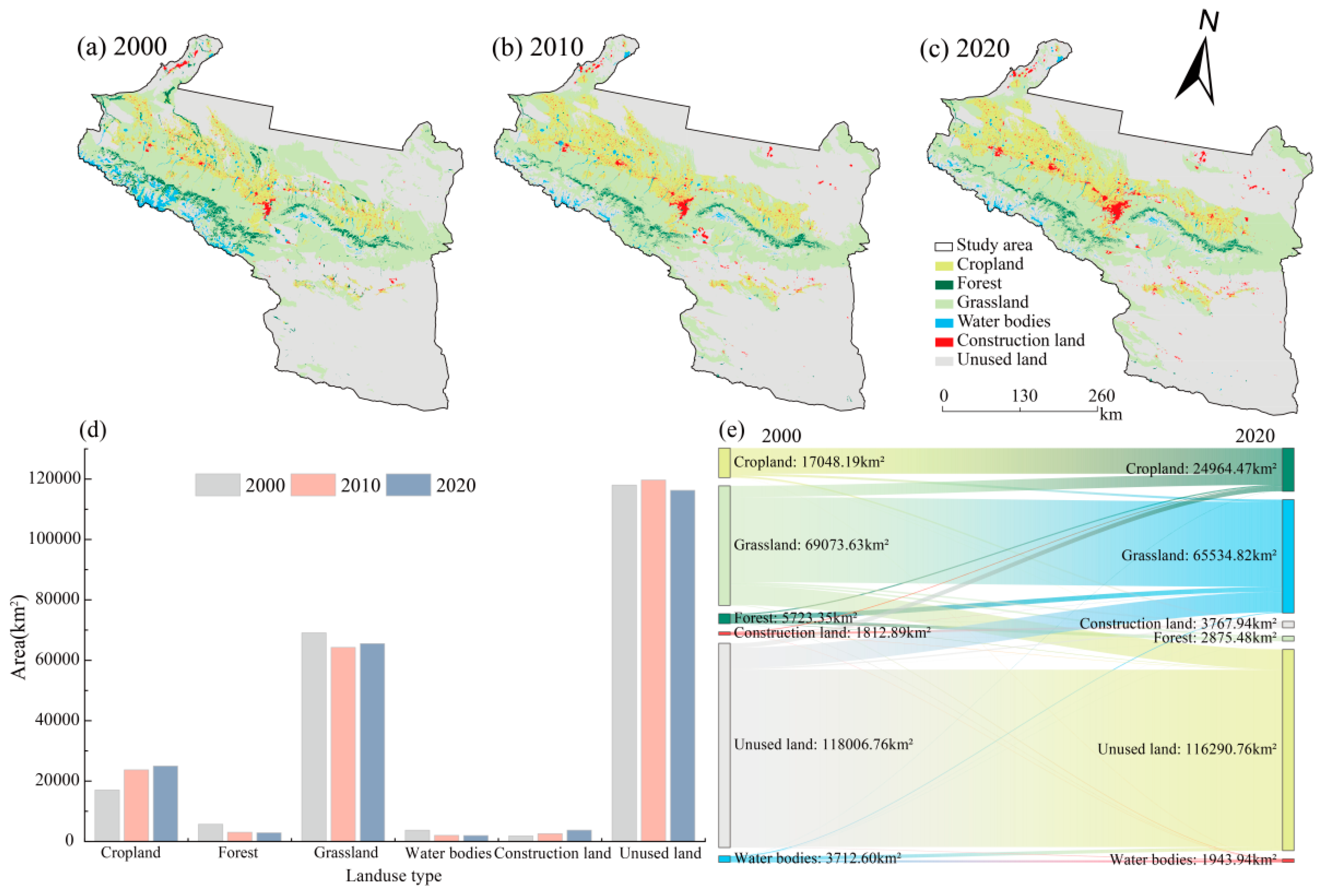
From 2000 to 2020, land use in the UANSTM was dominated by unused land and grassland, whereas cropland, construction land, water bodies, and forest occurred mainly as belts or patches (Figure 3a–c). Unused land was widely distributed in the northern and eastern parts of the study area and around oasis margins, forming the largest land-use category. Grassland was concentrated in the piedmont and mountain–oasis transition zones. Cropland was mainly located along the piedmont oasis belt and expanded markedly during the study period. Construction land was concentrated in oasis cities and surrounding areas, showing clustered, point-like, and locally corridor-like expansion (Figure 3a–c).

Land-use change was characterized by a stable background of unused land and grassland and a clear expansion of human-dominated land (Figure 3d; Table S1). In 2020, unused land and grassland together accounted for more than 84% of the study area, confirming the dominance of the mountain–oasis–desert landscape matrix. From 2000 to 2020, construction land showed the largest relative increase at 107.84%, while cropland expanded by 46.43%, mainly along the piedmont oasis belt. In contrast, forest and water bodies declined by 49.76% and 47.64%, respectively, indicating substantial contraction of key ecological land.

The timing and source of these changes were uneven. Most structural adjustment occurred during 2000–2010, whereas after 2010 cropland expansion slowed but construction land growth continued. The transition matrix shows that cropland and construction land expansion was mainly supplied by grassland and unused land conversion, with major transitions concentrated along oasis margins and urban expansion zones (Figure 3e; Table S2).

3.2. Spatiotemporal Evolution of LER and ESV

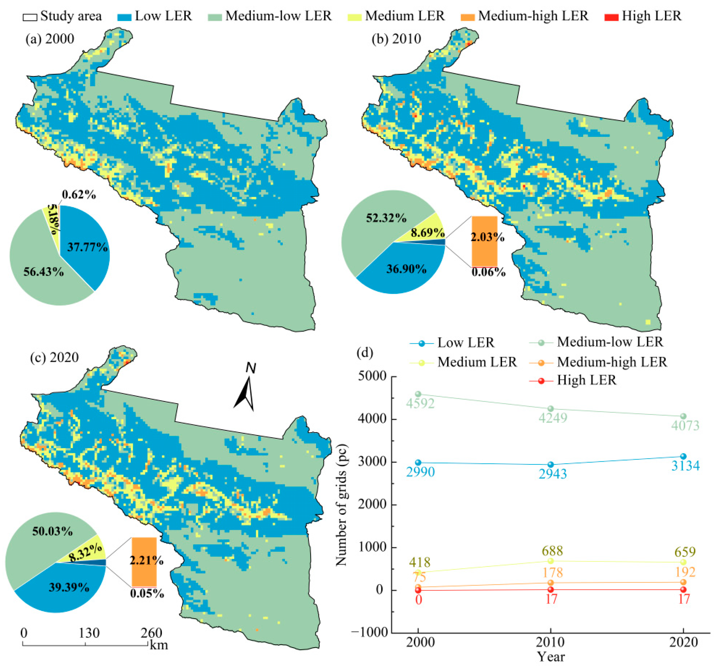
LER in the UANSTM was dominated by low- and medium-low-risk classes throughout 2000–2020, whereas medium-, medium-high-, and high-risk areas occupied relatively small proportions (Figure 4a–c). Low- and medium-low-risk areas were widely distributed across the study area. Medium- and medium-high-risk areas occurred mainly as strips or patches along the piedmont oasis belt, oasis margins, and local urban construction areas, while high-risk areas appeared only as scattered patches. The number of low-risk grid cells changed from 2990 in 2000 to 2943 in 2010 and 3134 in 2020. Medium-low-risk grid cells decreased continuously from 4592 to 4249 and then to 4073. By contrast, medium-high-risk grid cells increased from 75 to 178 and 192, and high-risk grid cells increased from 0 to 17 and remained at that level in 2020 (Figure 4d). Thus, the LER class structure was characterized by a decline in medium-low-risk areas, a later increase in low-risk areas, and a local expansion of medium-high-risk areas.

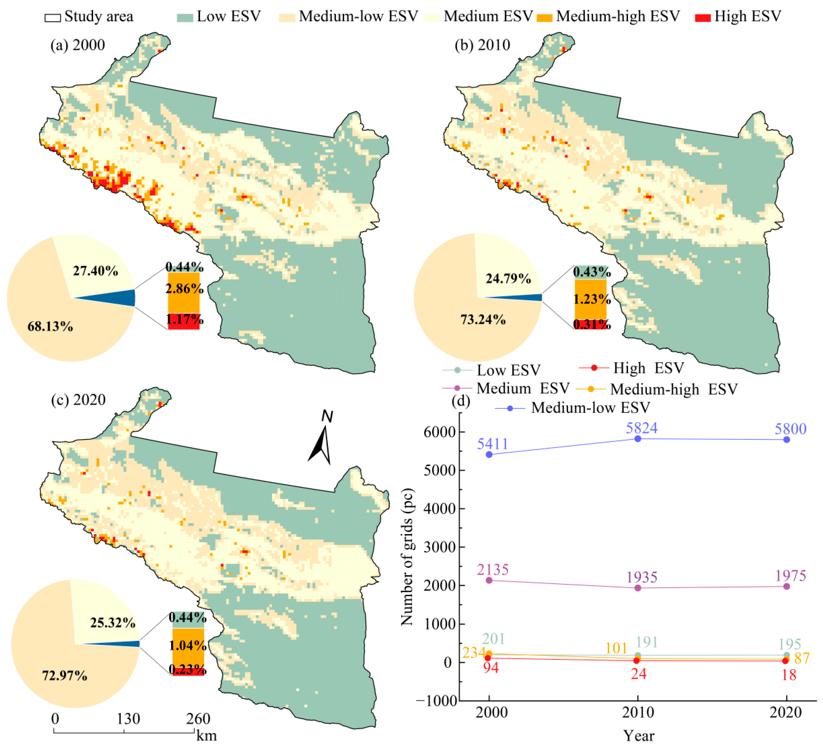
ESV was dominated by medium-low- and medium-value classes, whereas medium-high- and high-value areas were limited and occurred mainly as patches in mountain areas, river–lake systems, and local ecological patches (Figure 5a–c). Medium-low-ESV grid cells increased from 5411 in 2000 to 5824 in 2010 and remained high at 5800 in 2020. Medium-ESV grid cells decreased from 2135 to 1935 before increasing to 1975 in 2020. Medium-high- and high-ESV grid cells declined continuously, from 234 and 94 in 2000 to 87 and 18 in 2020, respectively (Figure 5d). These results indicate a persistent dominance of medium-low-ESV areas and a contraction of medium-high- and high-ESV zones.

Total ESV declined sharply during 2000–2010 and then recovered slightly by 2020 (

Table 3. Changes in ecosystem service value in the UANSTM from 2000 to 2020 (unit: billion CNY).

Land-Use Type	Cropland	Forest	Grassland	Water Bodies	Unused Land	Total Value
2000	32.16	50.75	272.15	120.46	36.63	512.16
2010	44.71	27.01	253.22	66.10	37.16	428.21
2020	47.09	25.50	258.21	63.07	36.10	429.97

). It decreased from 512.16 billion CNY in 2000 to 428.21 billion CNY in 2010 and then increased slightly to 429.97 billion CNY in 2020. Grassland was consistently the largest contributor, providing 272.15, 253.22, and 258.21 billion CNY in 2000, 2010, and 2020, respectively. ESV from water bodies and forest decreased substantially, from 120.46 and 50.75 billion CNY in 2000 to 63.07 and 25.50 billion CNY in 2020. Cropland ESV increased from 32.16 to 47.09 billion CNY. Overall, ESV loss was concentrated in 2000–2010, whereas 2010–2020 was characterized by relative stability and a slight recovery.

3.3. Static–Dynamic Coupling Zoning of LER and ESV

3.3.1. Evolution of Static Coupling Zones

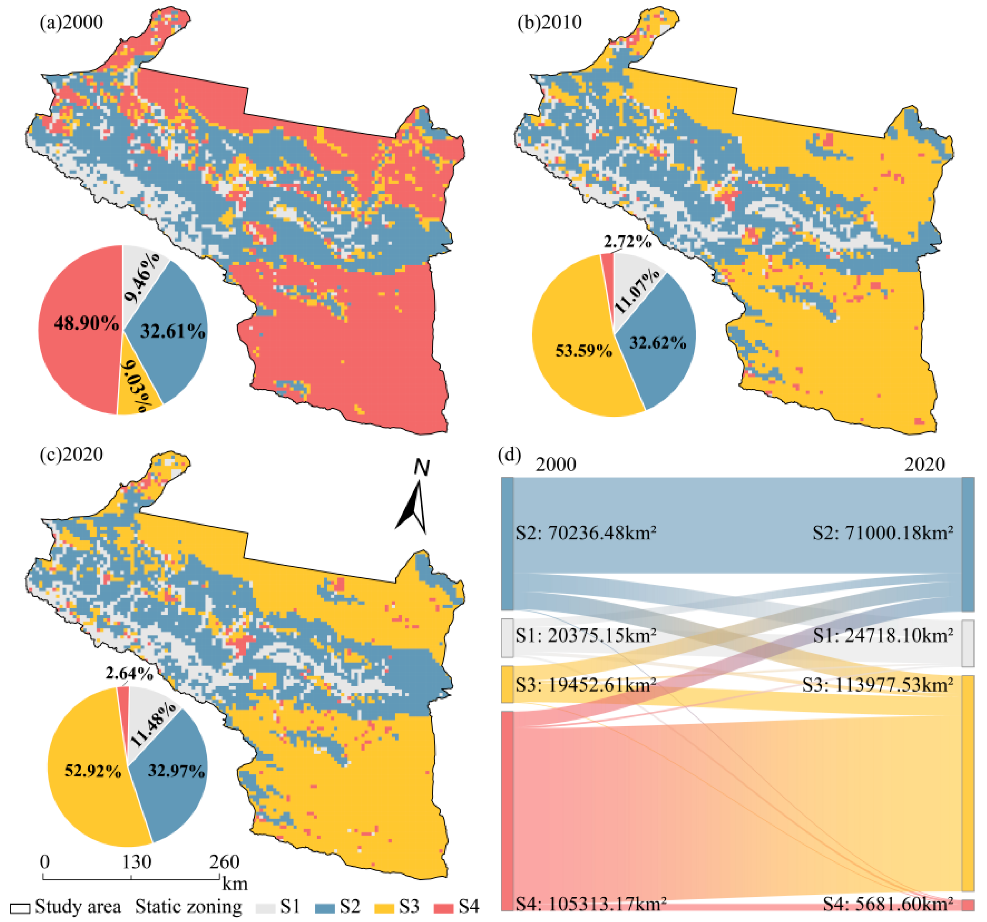
The static LER–ESV coupling structure shifted markedly from 2000 to 2020 (Figure 6a–d; Table S5). In 2000, the study area was dominated by S4 and S2, which accounted for 48.90% and 32.61%, respectively, indicating that high-risk–low-value mismatch areas and low-risk–high-value favorable areas coexisted. After 2010, S3 became the dominant type, accounting for 53.59% in 2010 and 52.92% in 2020. In contrast, S4 declined sharply from 48.90% in 2000 to 2.64% in 2020, showing a substantial reduction in high-risk–low-value mismatch areas. S2 remained relatively stable, ranging from 32.61% to 32.97% during 2000–2020, suggesting persistence of favorable low-risk–high-value areas. Notably, S1 increased from 9.46% to 11.48%, indicating that some high-ESV units were also exposed to high LER. The Sankey diagram further shows that the static transition was mainly driven by the large transfer out of S4 and the expansion of S3, rather than by a uniform improvement of all risk–service combinations.

3.3.2. Dynamic Trends of LER, ESV, and Comprehensive State

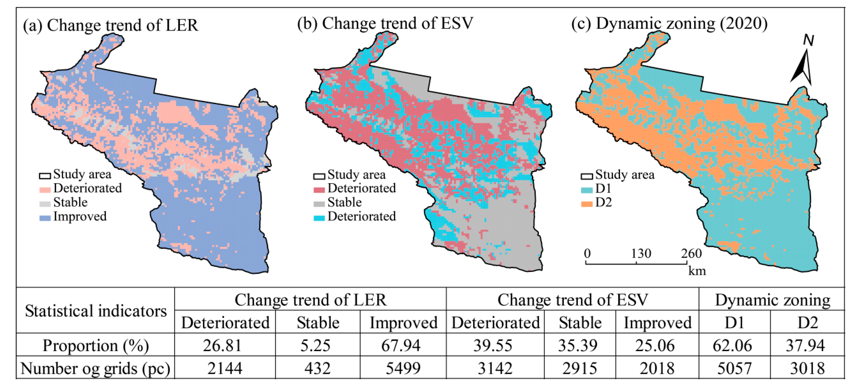
LER and ESV followed different trajectories from 2000 to 2020 (Figure 7a,b). LER was dominated by improvement: improved areas accounted for 67.94% of grid cells, corresponding to 5499 units, while deteriorated and stable areas accounted for 26.81% and 5.25%, corresponding to 2144 and 432 units (Figure 7a). In contrast, improved ESV areas accounted for only 25.06% of grid cells, whereas deteriorated and stable areas accounted for 39.55% and 35.39%, corresponding to 3142 and 2915 units (Figure 7b).

Dynamic zoning based on the comprehensive state trajectory showed that D1 accounted for 62.06% of grid cells, or 5057 units, whereas D2 accounted for 37.94%, or 3018 units (Figure 7c). D1 and D2 were spatially interspersed, but D1 covered a broader area, indicating that the comprehensive state of the study area was generally dominated by positive development. The persistence of D2 also suggests that localized degradation remained, especially where ESV decline offset LER improvement.

3.3.3. Integrated Management Zoning in 2020

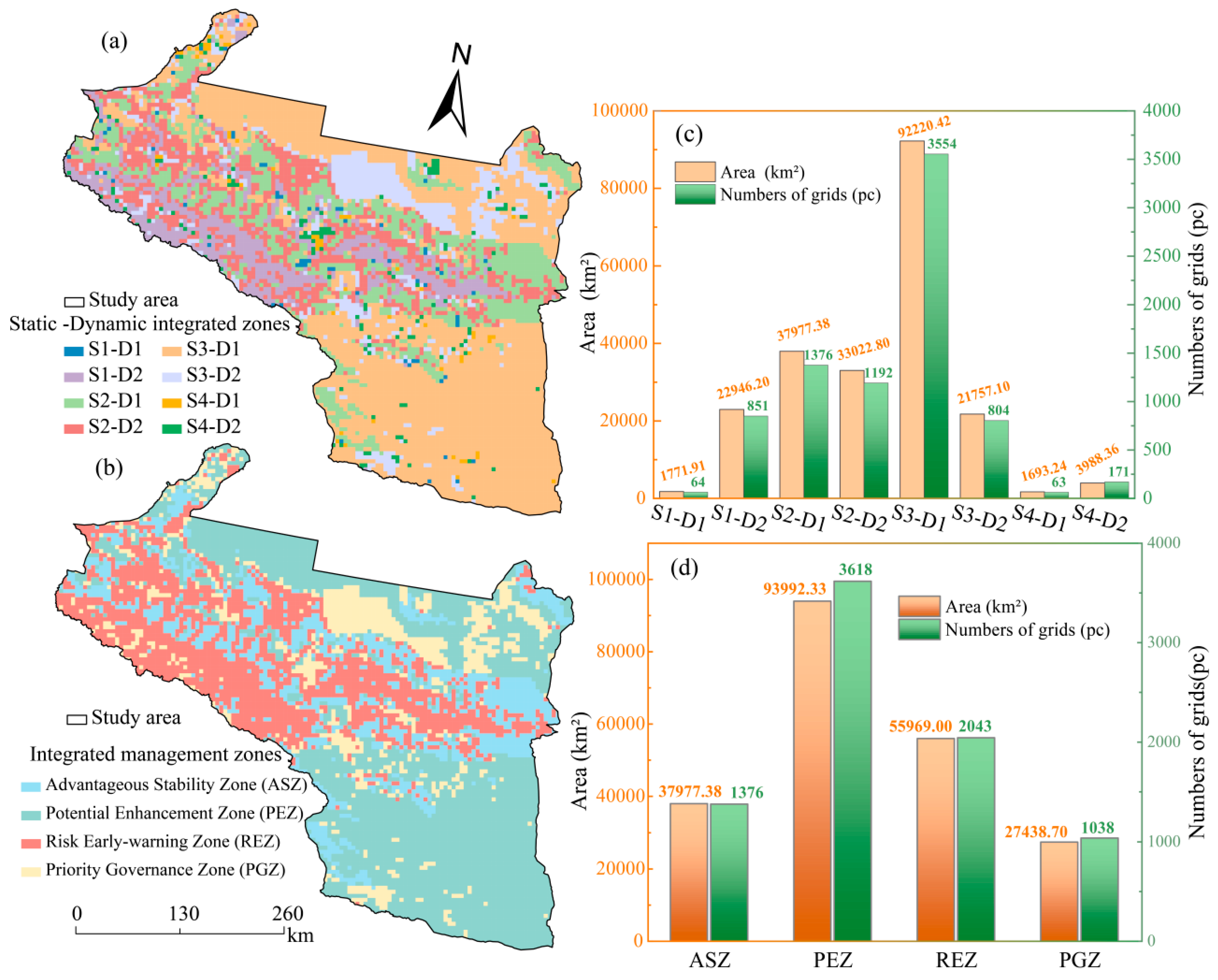
Overlaying the static and dynamic zones generated eight combined types in 2020 (Figure 8a,c; Table S7). S3-D1 was the dominant combination, covering 92,220.42 km², indicating that many low-risk–low-value areas had positive trajectories and could be enhanced rather than immediately governed as high-risk areas. S2-D1 represented the most favorable condition: low-risk, high-service value, and continued improvement. In contrast, D2-related combinations, especially S2-D2 and S1-D2, indicated areas where favorable or high-value states were already shifting toward degradation.

After aggregation, PEZ became the largest integrated management zone, accounting for 43.64% of the study area, followed by REZ at 25.99%, ASZ at 17.63%, and PGZ at 12.74% (Figure 8b,d). Ecologically, ASZ represents stable low-risk–high-value areas that should be maintained; PEZ represents improving areas with potential for service enhancement or risk reduction; REZ represents high-value or favorable-state areas with negative trajectories and should receive early warning; and PGZ represents low-value or high-risk mismatch areas requiring priority governance.

3.4. LER–ESV Zoning Responses Under 2030 Scenarios

3.4.1. Spatial Responses of Land Use, LER, and ESV

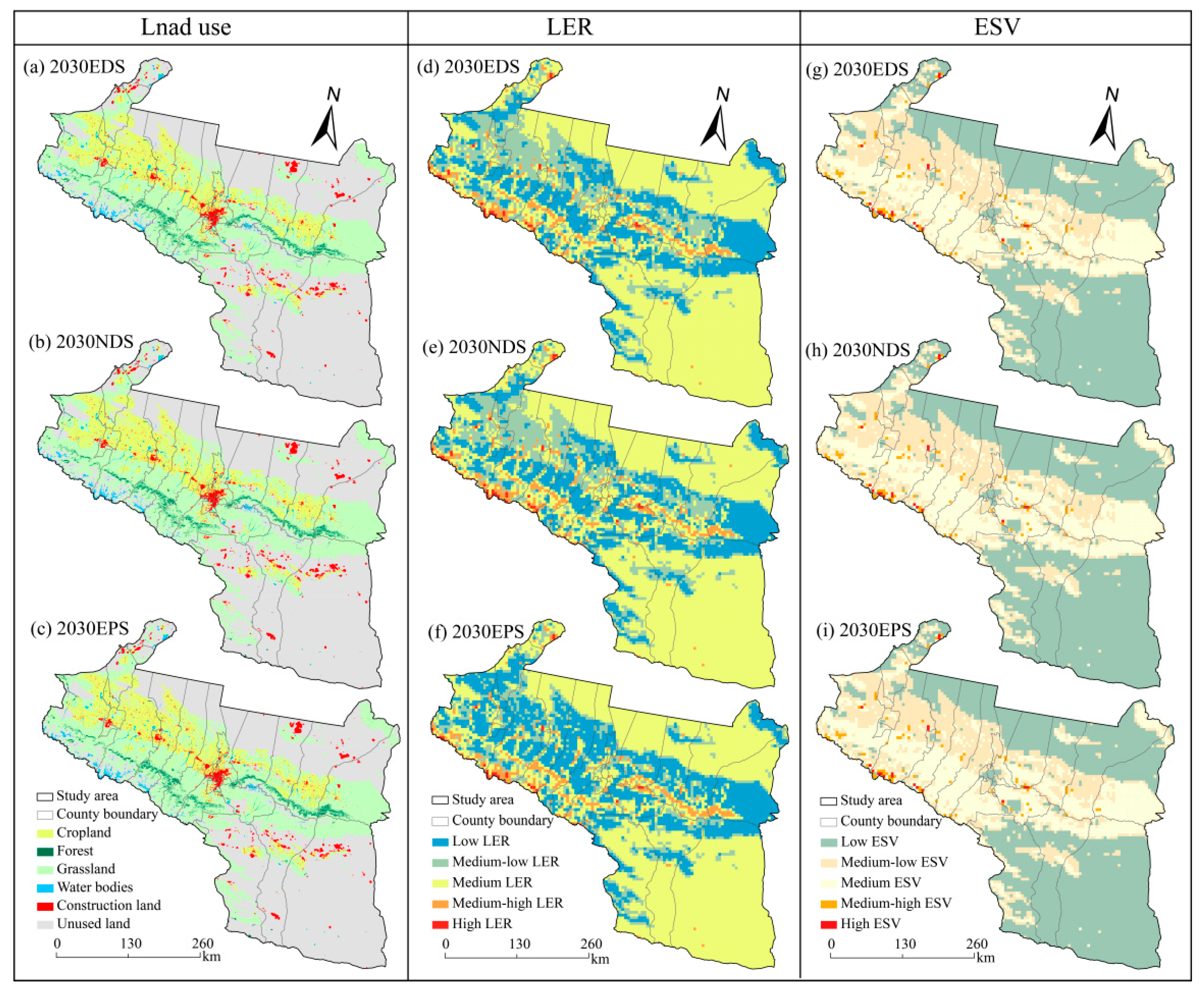
Under the EDS, NDS, and EPS in 2030, land-use patterns largely retained the mountain–oasis–desert structure, with unused land and grassland remaining dominant and cropland and construction land concentrated along the piedmont oasis belt and around urban nodes (Figure 9a–c). Overall differences among scenarios were limited, but local responses varied. Construction land expansion was most evident under EDS, intermediate under NDS, and relatively constrained under EPS (Figure 9a–c).

LER patterns were broadly similar across the three scenarios and were dominated by low-, medium-low-, and medium-risk classes. Medium-high- and high-risk areas were mainly distributed along the piedmont oasis belt, urban expansion margins, and local ecologically vulnerable zones (Figure 9d–f). ESV patterns also showed strong spatial continuity, with low- and medium-low-value areas remaining dominant. Medium-high- and high-ESV zones were mainly distributed in mountain areas, water bodies, and local ecological patches (Figure 9g–i). Overall, land use, LER, and ESV under the 2030 scenarios showed broad spatial continuity with local differentiation.

3.4.2. Responses of Static, Dynamic, and Integrated Management Zones

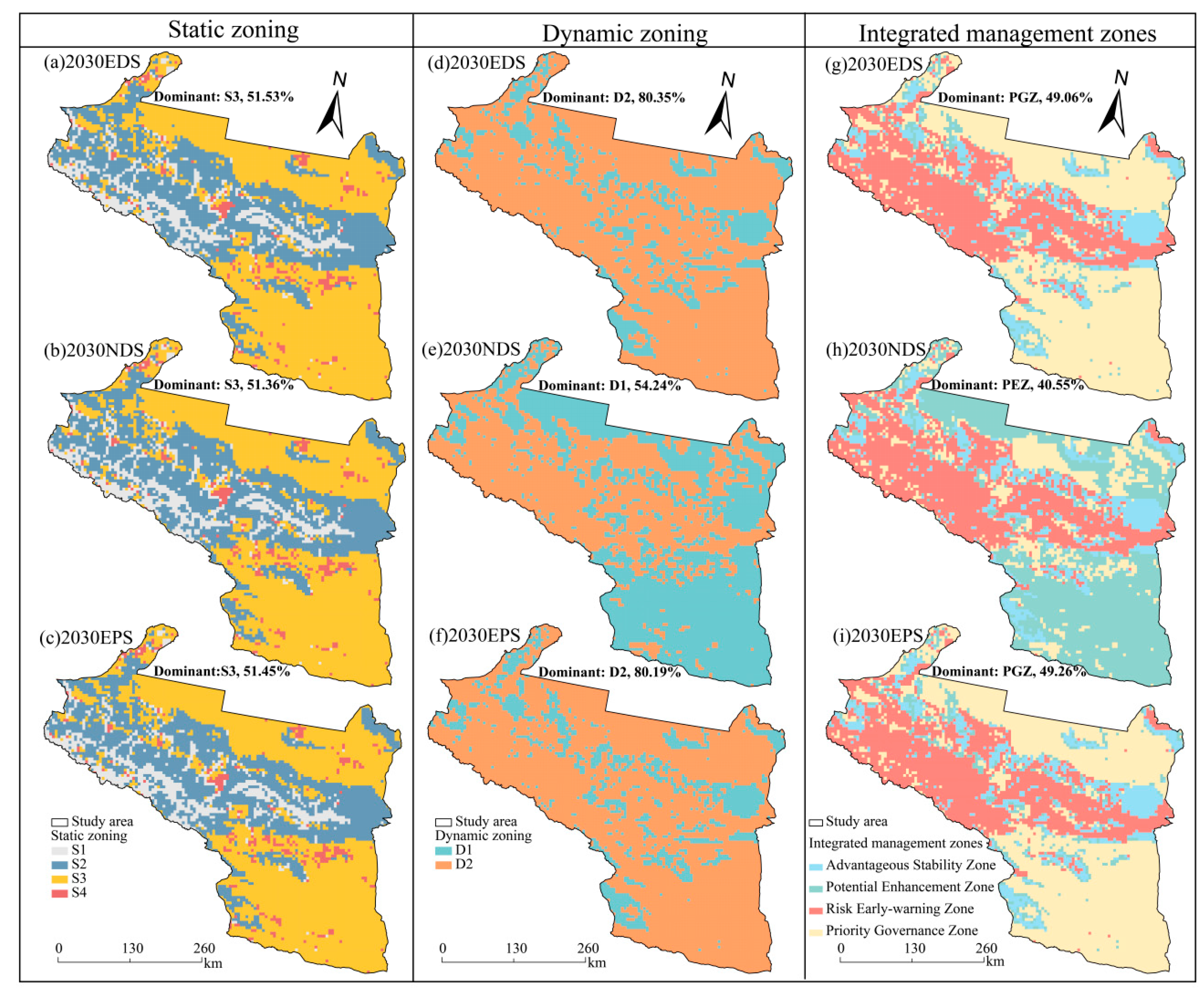
The static zoning structures under the three 2030 scenarios were similar, with S3 and S2 remaining dominant (Figure 10a–c; Table S8a). S3 accounted for 51.36–51.53% of the study area, and S2 accounted for 33.57–33.91%. S1 accounted for approximately 11%, while S4 accounted for 3.68–3.90%. Relative to 2020, S4 increased under all three scenarios, whereas S1 and S3 decreased slightly.

Dynamic zoning was more sensitive to scenario change than static zoning (Figure 10d–f; Table S8b). Under NDS, D1 accounted for 54.24% of the study area, indicating a stronger tendency toward comprehensive-state improvement. In contrast, D2 dominated under both EDS and EPS, accounting for 80.35% and 80.19%, respectively. This reveals an apparently counterintuitive pattern: the ecological protection scenario produced a dynamic zoning structure highly similar to the economic development scenario, rather than to NDS.

Integrated management zones further amplified this pattern (Figure 10g–i;

Table 4. Integrated management zones under the three 2030 scenarios.

Integrated Zone	EDS Area (km2; %)	EDS Grids	NDS Area (km2; %)	NDS Grids	EPS Area (km2; %)	EPS Grids
ASZ	26,441.89 (12.28)	957	27,770.94 (12.89)	1005	26,991.91 (12.53)	976
PEZ	14,580.18 (6.77)	564	87,333.42 (40.55)	3349	14,540.51 (6.75)	561
REZ	68,699.27 (31.90)	2506	67,207.47 (31.20)	2452	67,746.79 (31.45)	2472
PGZ	105,656.07 (49.06)	4048	33,065.58 (15.35)	1269	106,098.20 (49.26)	4066

). Under NDS, PEZ accounted for 40.55%, indicating that many units retained positive trajectories but still required service enhancement or risk reduction. By contrast, PGZ dominated under both EDS and EPS, accounting for 49.06% and 49.26%, respectively, but only 15.35% under NDS. Ecologically, this means that EDS and EPS shifted a much larger share of the landscape into priority governance status, where low service capacity, high risk pressure, or negative trajectories may threaten future risk–service balance. A preliminary explanation is that the 2030 integrated zoning was controlled mainly by the direction of comprehensive-state change relative to 2020, whereas static risk–service combinations remained comparatively stable.

4. Discussion

4.1. Land-Use Change as the Driver of LER–ESV Coupling

Land-use change provides the primary basis for LER–ESV coupling in the UANSTM. Land-use/cover change reshapes ecological risk by altering fragmentation, isolation, connectivity and disturbance intensity [4,19]. Construction land expansion raises LER by adding artificial patches, hard edges and connectivity breaks, especially along oasis cities and transport corridors. Cropland expansion has mixed effects: it can increase provisioning services, but when converted from grassland or unused land, it simplifies oasis-margin landscapes, strengthens edge disturbance and weakens regulating and supporting services. From 2000 to 2020, cropland and construction land expanded by 46.43% and 107.84%, whereas forest and water bodies declined by 49.76% and 47.64%. Concentrated along the piedmont oasis belt, oasis margins and urban fronts, these changes reorganized grassland, forest, water bodies and unused land, thereby changing LER composition and distribution.

ESV responded through a different pathway. While LER is mediated by landscape configuration and disturbance, ESV depends more directly on ecosystem area and value coefficients [6,7]. At broader scales, ecosystem extent strongly affects total ESV [22], and regional studies have also shown that land-use conversion can redistribute ESV among land-use types [23]. In arid oasis systems, water bodies, grassland and forest are critical because they sustain regulating and supporting services [24,25]. Their contraction therefore reduced service supply more than cropland expansion compensated. Total ESV declined from 512.16 to 429.97 billion CNY, mainly owing to losses in water bodies, forest and grassland. Thus, LER–ESV coupling was shaped by two linked but distinct pathways: landscape configuration affected risk, whereas service value affected ecosystem service supply. Their asynchronous responses explain risk–service mismatches: high-ESV ecological patches may still show high LER when fragmented or disturbed; low-risk unused land may remain low in ESV; and LER improvement may coexist with ESV decline when ecological land loss continues.

4.2. Added Value of Static–Dynamic Coupling Zoning

The main contribution of this framework is that it converts LER–ESV coupling from a static state description into a management-oriented diagnosis of state and trajectory. LER and ESV/ES represent complementary dimensions of ecological security: risk pressure and service provision. Assessing them separately weakens the interpretation of ecological protection needs and spatial governance priorities. Recent studies have therefore integrated LER with ESV or ES for ecological security assessment and zoning. Wang et al. [9] incorporated LER into ESV assessment to improve ecological security identification. Li et al. [10] used LER–ESV relationships for ecological zoning and scenario simulation. Liu and Tang [12] combined LER with multiple ESs to support zoning and management strategies.

However, most LER–ESV or LER–ES zoning studies remain state-based. Static quadrant zoning can identify low-risk–high-value, high-risk–high-value, low-risk–low-value and high-risk–low-value combinations, but not whether zones of the same type are improving, stable or degrading. This matters because ecosystem service trade-offs and synergies vary spatially [26], while ecosystem service bundles also change across landscapes and periods [27,28]. Ecological zoning therefore requires both current risk–service diagnosis and trajectory-based management prioritization.

The framework developed here addresses this limitation by integrating static state, dynamic trajectory and management zoning. Static zoning characterizes the annual LER–ESV risk–value combination, whereas dynamic zoning identifies whether the comprehensive state improved or degraded during 2000–2020. S1–S4 and D1/D2 therefore serve different diagnostic roles: S1–S4 identify the current risk–service combination, whereas D1/D2 identify improvement or degradation. Their overlay was aggregated into ASZ, PEZ, REZ and PGZ. Compared with static zoning alone, this framework separates areas with favorable current conditions and positive trajectories from areas with improvement potential, emerging warning signals or persistent governance pressure. It therefore avoids equating cross-sectional state with management priority.

The results support this approach. Static zoning suggested apparent improvement after 2010, as S3 became dominant and S4 contracted sharply. Yet dynamic analysis showed that LER improvement coexisted with ESV degradation, and degraded or stable ESV areas together exceeded 70%. Static zoning alone would overlook service-value loss or comprehensive-state decline, whereas dynamic trends alone would obscure current risk–value differences. Thus, ASZ, PEZ, REZ and PGZ are priorities derived from joint interpretation of current state and temporal trajectory, not simple LER–ESV overlay products. This is the key added value of the static–dynamic framework over state-only zoning.

4.3. Management Implications of the 2030 Scenarios

The 2030 scenario results show that future management priorities in the UANSTM depend not only on simulated land-use patterns but also on whether the integrated LER–ESV state improves or degrades. Multi-scenario land-use simulation has been used to evaluate future ecosystem service responses and land-use optimization [29], as well as ecological risk responses under alternative pathways [30]. Here, intPLUS/PLUS-based simulation supported scenario-based zoning updates for planning and governance control. The PLUS framework simulates land-use transitions under alternative pathways [20], and later scenario applications have linked simulated land-use change with ecological risk or ecosystem service responses [21,31]. The higher PEZ proportion under NDS indicates that a moderate pathway retained more ecological improvement space. These units were not yet stable high-service areas, but their positive trajectories suggest potential for proactive restoration and service enhancement. By contrast, PGZ dominance under EDS reflects the ecological cost of stronger development pressure, as construction and cropland expansion intensify fragmentation, hard edges and connectivity loss in oasis margins and urban fronts. EPS produced a counterintuitive pattern. Although it constrained construction expansion and better protected ecological land than EDS, it mainly limited further loss rather than restored degraded risk–service states. Construction land and cropland still increased, and water-body recovery remained insufficient, explaining why PGZ under EPS remained close to EDS. Overall, static zoning changed little across the three 2030 scenarios, whereas dynamic and integrated zoning differed markedly: PEZ reached 40.55% under NDS, while PGZ reached 49.06% and 49.26% under EDS and EPS. Scenario effects were therefore expressed mainly through comprehensive-state trajectories and management attributes, rather than large shifts in static risk–value combinations.

These results connect to current spatial governance instruments. Xinjiang’s territorial spatial planning emphasizes cultivated land and permanent basic farmland protection, ecological conservation redlines, urban development boundaries, mountain ecological barriers and oasis ecological rings [32]. National restoration policy promotes integrated management of mountains, rivers, forests, farmland, lakes and grasslands [33]. The integrated zones identified here can therefore link scenario simulation with territorial spatial control. ASZ should maintain low risk and stable service supply; PEZ should support grassland restoration, water-body rehabilitation, ecological farmland management and oasis-margin improvement; REZ requires monitoring and early warning; and PGZ should impose strict controls on construction expansion, inefficient land growth and fragmentation. The high PGZ proportion under EPS further shows that ecological protection cannot rely only on increasing ecological land or constraining construction land. Ecosystem-service-based ecological redline planning can help regulate development pressure [34], and China’s ecological redline policy also offers a spatial tool for strengthening conservation governance [35]. LER–ESV and LER–ES zoning can further identify priority areas for differentiated restoration and governance [10,12].

4.4. Uncertainties and Future Work

Several uncertainties remain. ESV was estimated using the unit-area value coefficient method, which supports regional and long-term comparison but relies on fixed land-use coefficients. This may underrepresent within-class heterogeneity in vegetation cover, degradation, productivity, ecological function, and water-body persistence. Future work should shift toward spatially adjusted coefficients. NDVI, FVC, and NPP describe vegetation greenness, cover, and productivity and can distinguish ESV differences within the same land-use/cover type [36]. Water-body persistence and seasonal dynamics could refine aquatic and wetland ESV. RSEI integrates greenness, wetness, dryness, and heat [37], while DHIs summarize cumulative productivity, minimum productivity, and intra-annual variability to complement habitat and biodiversity information [38,39]. Incorporating these indicators into ESV coefficient correction, LER vulnerability adjustment, and dynamic zoning would reduce the limitations of land-use-type-based assessment.

LER assessment and static–dynamic zoning are also sensitive to parameters, scale, and thresholds. Although this study used a disturbance–vulnerability–loss framework and 5 km × 5 km grids, landscape metric weights, vulnerability scores, grid resolution, and zoning thresholds may affect local classification [40]. Multi-scale comparison, weight sensitivity analysis, and threshold robustness testing are therefore needed to evaluate zoning stability.

The 2030 results should be interpreted as scenario-based projections rather than deterministic predictions. Although intPLUS validation showed high accuracy, EDS, NDS, and EPS depend on scenario-specific land-use demands and constraints. Future work could embed ecological conservation redlines, permanent basic farmland, urban development boundaries, and restoration projects in scenario rules and use longer time series to test zoning stability. Predictor collinearity and spatial dependence were not explicitly diagnosed. Although OA, Kappa, and FOM were used, VIF, residual Moran’s I, and spatial block cross-validation were not conducted. Collinearity can affect variable interpretation in ecological modeling [41], and ignoring spatial dependence may yield over-optimistic validation [42]. Adding these diagnostics would strengthen land-use suitability modeling and scenario simulation. These uncertainties may affect local zoning but not the regional patterns or comparative scenario insights identified here.

5. Conclusions

This study integrated land-use change analysis, LER and ESV assessment, static–dynamic coupling zoning, and intPLUS-based scenario simulation to diagnose the LER–ESV coupling pattern and its 2030 scenario responses in the UANSTM. Four main conclusions can be drawn:

(1)

From 2000 to 2020, land use in the study area remained dominated by unused land and grassland, but cropland and construction land expanded substantially, while forest and water bodies contracted markedly. Cropland and construction land increased by 46.43% and 107.84%, respectively, whereas forest and water bodies decreased by 49.76% and 47.64%. These changes were concentrated mainly along the piedmont oasis belt, oasis margins, and urban expansion areas.

(2)

LER and ESV showed pronounced spatial differentiation but evolved asynchronously. LER was dominated by low- and medium-low-risk classes, although medium-high-risk areas expanded. ESV was dominated by medium-low- and medium-value classes, whereas medium-high- and high-value zones continued to shrink. Total ESV decreased from 512.16 billion CNY in 2000 to 428.21 billion CNY in 2010, followed by a slight recovery to 429.97 billion CNY in 2020, indicating that ESV loss was concentrated mainly during 2000–2010.

(3)

Static–dynamic coupling zoning captured both risk–service matching or mismatching states and their temporal trajectories. Static zoning showed that S3 became dominant after 2010, whereas S4 contracted sharply; meanwhile, the persistence and expansion of S1 confirmed that high-risk areas were not necessarily low in ESV. Dynamic zoning showed that D1 and D2 accounted for 62.06% and 37.94%, respectively. In 2020, PEZ dominated the integrated management pattern, accounting for 43.64% of the study area, followed by REZ, ASZ, and PGZ at 25.99%, 17.63%, and 12.74%, respectively.

(4)

The 2030 scenario simulations showed limited changes in static zoning but strong responses in dynamic and integrated management zoning. PEZ accounted for 40.55% under NDS, whereas PGZ accounted for 49.06% and 49.26% under EDS and EPS, respectively. These results suggest that alternative development pathways reshape management-zone attributes mainly by altering the direction of comprehensive-state change. The proposed static–dynamic coupling and scenario simulation framework is transferable beyond the UANSTM to other arid urban agglomerations, mountain–oasis–desert systems, and rapidly urbanizing ecologically fragile regions. By separating current risk–service state from temporal trajectory and updating zoning under alternative scenarios, the framework can support comparative diagnosis of risk–service mismatches and differentiated ecological management across regions facing similar land-use transition pressures.

References

1. Seto, K.C.; Güneralp, B.; Hutyra, L.R. Global forecasts of urban expansion to 2030 and direct impacts on biodiversity and carbon pools. Proc. Natl. Acad. Sci. USA 2012, 109, 16083–16088. [Google Scholar] [CrossRef] [Scilit] [PubMed]
2. Newbold, T.; Hudson, L.N.; Hill, S.L.L.; Contu, S.; Lysenko, I.; Senior, R.A.; Börger, L.; Bennett, D.J.; Choimes, A.; Collen, B.; et al. Global effects of land use on local terrestrial biodiversity. Nature 2015, 520, 45–50. [Google Scholar] [CrossRef] [Scilit] [PubMed]
3. Ouyang, Z.; Zheng, H.; Xiao, Y.; Polasky, S.; Liu, J.; Xu, W.; Wang, Q.; Zhang, L.; Xiao, Y.; Rao, E.; et al. Improvements in ecosystem services from investments in natural capital. Science 2016, 352, 1455–1459. [Google Scholar] [CrossRef] [Scilit] [PubMed]
4. Zhang, W.; Chang, W.J.; Zhu, Z.; Hui, Z. Landscape ecological risk assessment of Chinese coastal cities based on land use change. Appl. Geogr. 2020, 117, 102174. [Google Scholar] [CrossRef] [Scilit]
5. Lin, X.; Wang, Z. Landscape ecological risk assessment and its driving factors of multi-mountainous city. Ecol. Indic. 2023, 146, 109823. [Google Scholar] [CrossRef] [Scilit]
6. de Groot, R.; Brander, L.; van der Ploeg, S.; Costanza, R.; Bernard, F.; Braat, L.; Christie, M.; Crossman, N.; Ghermandi, A.; Hein, L.; et al. Global estimates of the value of ecosystems and their services in monetary units. Ecosyst. Serv. 2012, 1, 50–61. [Google Scholar] [CrossRef] [Scilit]
7. Xie, G.; Zhang, C.; Zhen, L.; Zhang, L. Dynamic changes in the value of China’s ecosystem services. Ecosyst. Serv. 2017, 26, 146–154. [Google Scholar] [CrossRef] [Scilit]
8. Burkhard, B.; Kroll, F.; Nedkov, S.; Müller, F. Mapping ecosystem service supply, demand and budgets. Ecol. Indic. 2012, 21, 17–29. [Google Scholar] [CrossRef] [Scilit]
9. Wang, L.-J.; Luo, G.-Y.; Ma, S.; Wang, H.-Y.; Jiang, J.; Zhang, J.-G. Integrating landscape ecological risk into ecosystem service value assessment: A case study of Nanjing City, China. Ecol. Indic. 2023, 154, 110625. [Google Scholar] [CrossRef] [Scilit]
10. Li, J.; Hu, D.; Wang, Y.; Chu, J.; Yin, H.; Ma, M. Study of identification and simulation of ecological zoning through integration of landscape ecological risk and ecosystem service value. Sustain. Cities Soc. 2024, 107, 105442. [Google Scholar] [CrossRef] [Scilit]
11. Xiong, H.; Hu, Y.; Li, X.; Liu, Y.; Zhang, L. Integrating landscape ecological risks and ecosystem service values into the ecological security pattern identification of Wuhan urban agglomeration. Int. J. Environ. Res. Public Health 2023, 20, 2792. [Google Scholar] [CrossRef] [Scilit] [PubMed]
12. Liu, H.; Tang, D. Ecological zoning and ecosystem management based on landscape ecological risk and ecosystem services: A case study in the Wuling Mountain Area. Ecol. Indic. 2024, 166, 112421. [Google Scholar] [CrossRef] [Scilit]
13. Fang, C.; Gao, Q.; Zhang, X.; Cheng, W. Spatiotemporal characteristics of the expansion of an urban agglomeration and its effect on the eco-environment: Case study on the northern slope of the Tianshan Mountains. Sci. China Earth Sci. 2019, 62, 1461–1472. [Google Scholar] [CrossRef] [Scilit]
14. Yan, Y.; Chai, Z.; Yang, X.; Simayi, Z.; Yang, S. The temporal and spatial changes of the ecological environment quality of the urban agglomeration on the northern slope of Tianshan Mountain and the influencing factors. Ecol. Indic. 2021, 133, 108380. [Google Scholar] [CrossRef] [Scilit]
15. Aizizi, Y.; Kasimu, A.; Liang, H.; Zhang, X.; Zhao, Y.; Wei, B. Evaluation of ecological space and ecological quality changes in urban agglomeration on the northern slope of the Tianshan Mountains. Ecol. Indic. 2023, 146, 109896. [Google Scholar] [CrossRef] [Scilit]
16. Huang, S.; Song, W.; Gao, H.; Cao, C.; Li, J.; Liu, B.; Yu, H.; Li, S.; Wei, X.; Sheng, S. Association between ecological risks and ecosystem services in an urban agglomeration in arid China. Front. Environ. Sci. 2023, 10, 1101080. [Google Scholar] [CrossRef] [Scilit]
17. Song, X.; Chen, F.; Sun, Y.; Ma, J.; Yang, Y.; Shi, G. Effects of land utilization transformation on ecosystem services in urban agglomeration on the northern slope of the Tianshan Mountains, China. Ecol. Indic. 2024, 162, 112046. [Google Scholar] [CrossRef] [Scilit]
18. Jing, X.; He, Y.; Sun, Y.; Wang, M.; Wang, X. Spatial–temporal divergence and coupling analysis of land use change and ecosystem service value in the Yangtze River Delta Urban Agglomeration. Sustainability 2024, 16, 6624. [Google Scholar] [CrossRef] [Scilit]
19. Cheng, Y.; Li, J.; Wang, J.; Li, Y. Assessment and prediction of landscape ecological risk based on land use change in Xinjiang, China. Land 2023, 12, 895. [Google Scholar] [CrossRef] [Scilit]
20. Liang, X.; Guan, Q.; Clarke, K.C.; Liu, S.; Wang, B.; Yao, Y. Understanding the drivers of sustainable land expansion using a patch-generating land use simulation (PLUS) model: A case study in Wuhan, China. Comput. Environ. Urban Syst. 2021, 85, 101569. [Google Scholar] [CrossRef] [Scilit]
21. Gao, L.; Tao, F.; Liu, R.; Wang, Z.; Leng, H.; Zhou, T. Multi-scenario simulation and ecological risk analysis of land use based on the PLUS model: A case study of Nanjing. Sustain. Cities Soc. 2022, 85, 104055. [Google Scholar] [CrossRef] [Scilit]
22. Costanza, R.; de Groot, R.S.; Sutton, P.; van der Ploeg, S.; Anderson, S.J.; Kubiszewski, I.; Farber, S.; Turner, R.K. Changes in the global value of ecosystem services. Glob. Environ. Change 2014, 26, 152–158. [Google Scholar] [CrossRef] [Scilit]
23. Guo, P.; Zhang, F.; Wang, H. The response of ecosystem service value to land use change in the middle and lower Yellow River: A case study of the Henan section. Ecol. Indic. 2022, 140, 109019. [Google Scholar] [CrossRef] [Scilit]
24. Mamat, A.; Halik, Ü.; Rouzi, A. Variations of ecosystem service value in response to land-use change in the Kashgar Region, Northwest China. Sustainability 2018, 10, 200. [Google Scholar] [CrossRef] [Scilit]
25. Li, X.; Wu, C. Sensitivity assessment and simulation of ecosystem services in response to land use change in arid regions: Empirical evidence from Xinjiang, China. Ecol. Indic. 2025, 171, 113150. [Google Scholar] [CrossRef] [Scilit]
26. Bennett, E.M.; Peterson, G.D.; Gordon, L.J. Understanding relationships among multiple ecosystem services. Ecol. Lett. 2009, 12, 1394–1404. [Google Scholar] [CrossRef] [Scilit] [PubMed]
27. Raudsepp-Hearne, C.; Peterson, G.D.; Bennett, E.M. Ecosystem service bundles for analyzing tradeoffs in diverse landscapes. Proc. Natl. Acad. Sci. USA 2010, 107, 5242–5247. [Google Scholar] [CrossRef] [Scilit] [PubMed]
28. Meacham, M.; Norström, A.V.; Peterson, G.D.; Andersson, E.; Bennett, E.M.; Biggs, R.; Crouzat, E.; Cord, A.F.; Enfors, E.; Felipe-Lucia, M.R.; et al. Advancing research on ecosystem service bundles for comparative assessments and synthesis. Ecosyst. People 2022, 18, 99–111. [Google Scholar] [CrossRef] [Scilit]
29. Li, C.; Wu, Y.; Gao, B.; Zheng, K.; Wu, Y.; Li, C. Multi-scenario simulation of ecosystem service value for optimization of land use in the Sichuan–Yunnan ecological barrier, China. Ecol. Indic. 2021, 132, 108328. [Google Scholar] [CrossRef] [Scilit]
30. Gan, L.; Halik, Ü.; Shi, L.; Welp, M. Multi-scenario dynamic prediction of ecological risk assessment in an arid area of northwest China. Ecol. Indic. 2023, 154, 110727. [Google Scholar] [CrossRef] [Scilit]
31. Liu, X.; Li, Y.; Lu, J.; Song, T.; Zhang, S. Urban growth simulation guided by ecosystem service trade-offs in Wuhan metropolitan area: Methods and implications for spatial planning. Ecol. Indic. 2024, 167, 112687. [Google Scholar] [CrossRef] [Scilit]
32. People’s Government of Xinjiang Uygur Autonomous Region. Territorial Spatial Planning of Xinjiang Uygur Autonomous Region (2021–2035); People’s Government of Xinjiang Uygur Autonomous Region: Urumqi, China, 2024.
33. National Development and Reform Commission; Ministry of Natural Resources. Master Plan for Major Projects for the Protection and Restoration of Important National Ecosystems (2021–2035); National Development and Reform Commission: Beijing, China; Ministry of Natural Resources: Beijing, China, 2020.
34. Bai, Y.; Wong, C.P.; Jiang, B.; Hughes, A.C.; Wang, M.; Wang, Q. Developing China’s ecological redline policy using ecosystem services assessments for land use planning. Nat. Commun. 2018, 9, 3034. [Google Scholar] [CrossRef] [Scilit] [PubMed]
35. Choi, C.-Y.; Shi, X.; Shi, J.; Gan, X.; Wen, C.; Zhang, J.; Jackson, M.V.; Fuller, R.A.; Gibson, L. China’s ecological conservation redline policy is a new opportunity to meet post-2020 protected area targets. Conserv. Lett. 2022, 15, e12853. [Google Scholar] [CrossRef] [Scilit]
36. Zhou, F.C.; Han, X.; Tang, S.; Song, X.; Wang, H. An improved model for evaluating ecosystem service values using land use/cover and vegetation parameters. J. Meteorol. Res. 2021, 35, 148–156. [Google Scholar] [CrossRef] [Scilit]
37. Liu, P.; Ren, C.; Yu, W.; Ren, H.; Xia, C. Exploring the ecological quality and its drivers based on annual remote sensing ecological index and multisource data in Northeast China. Ecol. Indic. 2023, 154, 110589. [Google Scholar] [CrossRef] [Scilit]
38. Hobi, M.L.; Dubinin, M.; Graham, C.H.; Coops, N.C.; Clayton, M.K.; Pidgeon, A.M.; Radeloff, V.C. A comparison of Dynamic Habitat Indices derived from different MODIS products as predictors of avian species richness. Remote Sens. Environ. 2017, 195, 142–152. [Google Scholar] [CrossRef] [Scilit]
39. Radeloff, V.C.; Dubinin, M.; Coops, N.C.; Allen, A.M.; Brooks, T.M.; Clayton, M.K.; Costa, G.C.; Graham, C.H.; Helmers, D.P.; Ives, A.R.; et al. The Dynamic Habitat Indices (DHIs) from MODIS and global biodiversity. Remote Sens. Environ. 2019, 222, 204–214. [Google Scholar] [CrossRef] [Scilit]
40. Ai, J.; Yu, K.; Zeng, Z.; Yang, L.; Liu, Y.; Liu, J. Assessing the dynamic landscape ecological risk and its driving forces in an island city based on optimal spatial scales: Haitan Island, China. Ecol. Indic. 2022, 137, 108771. [Google Scholar] [CrossRef] [Scilit]
41. Dormann, C.F.; Elith, J.; Bacher, S.; Buchmann, C.; Carl, G.; Carré, G.C.G.; García Márquez, J.R.; Gruber, B.; Lafourcade, B.; Leitão, P.J.; et al. Collinearity: A review of methods to deal with it and a simulation study evaluating their performance. Ecography 2013, 36, 27–46. [Google Scholar] [CrossRef] [Scilit]
42. Roberts, D.R.; Bahn, V.; Ciuti, S.; Boyce, M.S.; Elith, J.; Guillera-Arroita, G.; Hauenstein, S.; Lahoz-Monfort, J.J.; Schröder, B.; Thuiller, W.; et al. Cross-validation strategies for data with temporal, spatial, hierarchical, or phylogenetic structure. Ecography 2017, 40, 913–929. [Google Scholar] [CrossRef] [Scilit]
Figure 1. Location and geographical setting of the urban agglomeration on the northern slope of the Tianshan Mountains.
Land 15 01302 g001
Figure 2. Research workflow.
Land 15 01302 g002
Figure 3. Land-use pattern and transition characteristics in the UANSTM from 2000 to 2020. (ac) Spatial distribution of land use in 2000, 2010, and 2020; (d) changes in the area of different land-use types from 2000 to 2020; (e) Sankey diagram of land-use transitions from 2000 to 2020.
Land 15 01302 g003
Figure 4. Spatial distribution and class structure of LER in the UANSTM from 2000 to 2020. (ac) Spatial distribution and area proportions of LER classes in 2000, 2010, and 2020; (d) changes in the number of evaluation units for different LER classes from 2000 to 2020.
Land 15 01302 g004
Figure 5. Spatial distribution and class structure of ESV in the UANSTM from 2000 to 2020. (ac) Spatial distribution and area proportions of ESV classes in 2000, 2010, and 2020; (d) changes in the number of evaluation units for different ESV classes from 2000 to 2020.
Land 15 01302 g005
Figure 6. Spatial pattern and structural evolution of static LER–ESV coupling zones in the UANSTM from 2000 to 2020. (ac) Spatial distribution and area proportions of static coupling zones in 2000, 2010, and 2020; (d) Sankey diagram of area transfers among static coupling zones from 2000 to 2020. Note: Percentages may not sum exactly to 100.00% because of rounding to two decimal places.
Land 15 01302 g006
Figure 7. Spatial patterns of LER and ESV change trends and dynamic zoning in the UANSTM from 2000 to 2020. (a) Spatial pattern of LER change trends from 2000 to 2020; (b) spatial pattern of ESV change trends from 2000 to 2020; (c) spatial pattern of dynamic zoning from 2000 to 2020.
Land 15 01302 g007
Figure 8. Spatial pattern and type structure of static–dynamic integrated zoning in the UANSTM in 2020. (a) Spatial pattern of eight static–dynamic combined zones; (b) spatial pattern of four integrated zones; (c) area and number of evaluation units of eight static–dynamic combined zones; (d) area and number of evaluation units of four integrated zones.
Land 15 01302 g008
Figure 9. Land-use pattern and spatial distributions of LER and ESV under three scenarios in the UANSTM in 2030. (ac) Land-use patterns under EDS, NDS, and EPS; (df) spatial distributions of LER under EDS, NDS, and EPS; (gi) spatial distributions of ESV under EDS, NDS, and EPS. Note: EDS, NDS, and EPS denote the economic development scenario, natural development scenario, and ecological protection scenario, respectively.
Land 15 01302 g009
Figure 10. Spatial patterns of static zoning, dynamic zoning, and integrated zoning under three scenarios in the UANSTM in 2030. (ac) Spatial patterns of static zoning under EDS, NDS, and EPS; (df) spatial patterns of dynamic zoning under EDS, NDS, and EPS; (gi) spatial patterns of integrated zoning under EDS, NDS, and EPS. Note: EDS, NDS, and EPS denote the economic development scenario, natural development scenario, and ecological protection scenario, respectively.
Land 15 01302 g010