Identifying Homogeneous Regions for Flash Floods Using Graph Clustering Neural Networks in Jiangxi Province, China

Abstract

Identifying homogeneous flash flood regions through regionalization is essential for effective mitigation and prevention. However, most existing regionalization methods focus primarily on attribute similarity (e.g., meteorological and underlying factors), while ignoring structural similarity that reflects topological network and flow relationships among catchments. In this study, we developed a new graph-clustering-neural-network-based flash flood regionalization (GFFR) method to address these limitations and improve the homogeneous region delineation. Catchments were first represented as a directed graph. Within GFFR, we then designed a graph convolutional autoencoder to learn latent representations that capture both catchment structure and attributes, while a decoder grouped the catchments into clusters. GFFR was applied in Jiangxi province, China, where it outperformed three typical clustering methods. Historical flash flood events were used to validate the GFFR map, presenting strong spatial consistency with dense event clusters and achieving a determinant power of 81%. Furthermore, the GFFR achieved a 24% higher determinant power than the average performance of the three compared methods. Overall, GFFR provides a valuable tool for flash flood regionalization, while the delineated regions offer critical guidance for governmental flash flood prevention and mitigation strategies.

1. Introduction

Flash floods are one of the most lethal natural disasters in the world, frequently causing severe loss of life and extensive damage to both natural and human-made resources [1,2,3,4]. Identifying homogeneous regions of flash floods is crucial for effective mitigation and prevention [5,6,7]. Homogeneous regions with similar flash flood generation mechanisms are particularly valuable for risk assessment and for regionalizing parameters in flash flood forecasting models [7,8,9,10,11,12,13]. Within such homogeneous regions, unified flash flood mitigation strategies can be formulated, while calibrated parameters derived from gauged catchments can be reliably transferred to ungauged counterparts for flash flood prediction.

Delineating homogeneous regions of flash flood is a typical regionalization task that aims to identify regions with similar flash flood generation conditions and responses. Since flash flood occurrence is closely associated with physical and environmental controls such as rainfall, topography, and drainage conditions, regionalization provides an effective way to characterize spatial homogeneity and support risk reduction and disaster prevention [14]. It produces a regionalization map by partitioning a geographical area into several distinct and non-overlapping homogeneous regions, where regional homogeneity is defined by similarity in the physical and environmental controls governing flash flood occurrence (e.g., rainfall and topography) [5,13,15,16,17]. Regionalization commonly leverages clustering algorithms to capture and quantify fundamental geographical principles [16,18,19,20,21]. As a specialized form of spatial clustering, regionalization groups spatial units into regions based on similarity while accounting for regional heterogeneity [17,22,23]. Clustering algorithms have been widely applied to delineate geographical regions in various domains, including climate regions [24,25], ecological zones [26,27], hydrologic divisions [28,29], and flash flood regions [5,30,31].

Traditional cluster analysis-based regionalization methods can be categorized into spatially implicit and spatially explicit approaches, depending on how spatial constraints are addressed [17,32]. Spatially implicit approaches primarily employ non-spatial clustering algorithms [17,32], such as the K-means algorithm [33,34]. Because these methods focus solely on attribute homogeneity, additional post-processing is often required to maintain spatial continuity. Such post-processing typically relies on expert knowledge, introducing subjectivity and reducing the cohesiveness of regions [17,32]. In contrast, spatially explicit methods incorporate spatial constraints (e.g., rules or conditions) directly into the clustering process to ensure spatial contiguity [32], such as SKATER [35] and Heuristic Distillation [36].

Recent advances in graph clustering neural networks (GCNNs) have revolutionized traditional clustering algorithms due to their strong capability to represent and learn both attribute and structure features [37,38,39,40,41]. GCNNs, which are neural networks designed to partition graph into homogeneous and non-overlapping subgraphs, can automatically extract important features during the encoding process, thereby avoiding the need for manual feature importance analysis required in traditional machine learning algorithms [37,39,42]. Moreover, GCNNs generate abstract representations of node features, which enables the capture of complex relationships and patterns among nodes and their neighborhoods. Tian et al. [43] initially applied deep learning models to graph clustering problems by leveraging an autoencoder for feature extraction, achieving significantly better results than conventional clustering algorithms. Since then, numerous GCNN variants have been developed, which can be broadly categorized into two groups [38,44]. The first group integrates both structural and attribute information in graph datasets, such as Deep Graph Structured Clustering Network [45] and Attention-based Graph Clustering Network [46]. The second group concentrates on improving node representations, such as Embedding Graph Auto-Encoder [39] and Deep Fusion Clustering Network [47]. GCNNs offer novel means for jointly representing the attributes and structures of spatial units, making them particularly valuable for clustering tasks. By applying convolution operations on graph structures, GCNNs can effectively encode both attribute and explicit structural information (e.g., flow direction and network topology) of spatial units, which is crucial for exploring spatial relationships [48,49]. These advances demonstrate the potential of GCNNs to enhance the performance of geographical regionalization.

However, most existing methods still rely on traditional spatial implicit regionalization techniques, which struggle to simultaneously represent the attributes and structural relationships of catchments affected by flash floods [5,50]. Meanwhile, the potential of GCNNs in flash flood regionalization remains largely unexplored, despite their capability to more effectively capture both the attributes and structures of flash flood-prone catchments.

To this end, this study aims to propose a novel graph-clustering-neural-network-based flash flood regionalization method (GFFR) that explicitly incorporates both attribute and structural similarities to improve the homogeneous region delineation. Its performance is validated in Jiangxi province, China, and compared with three existing methods.

2. Materials and Methods

2.1. Case Study Area

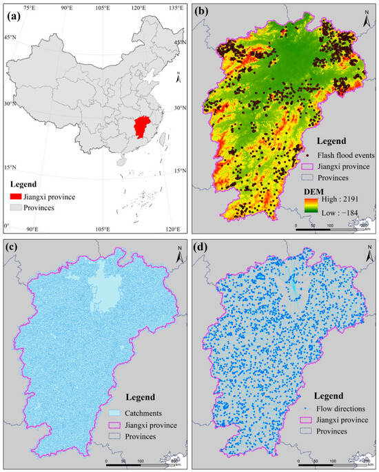
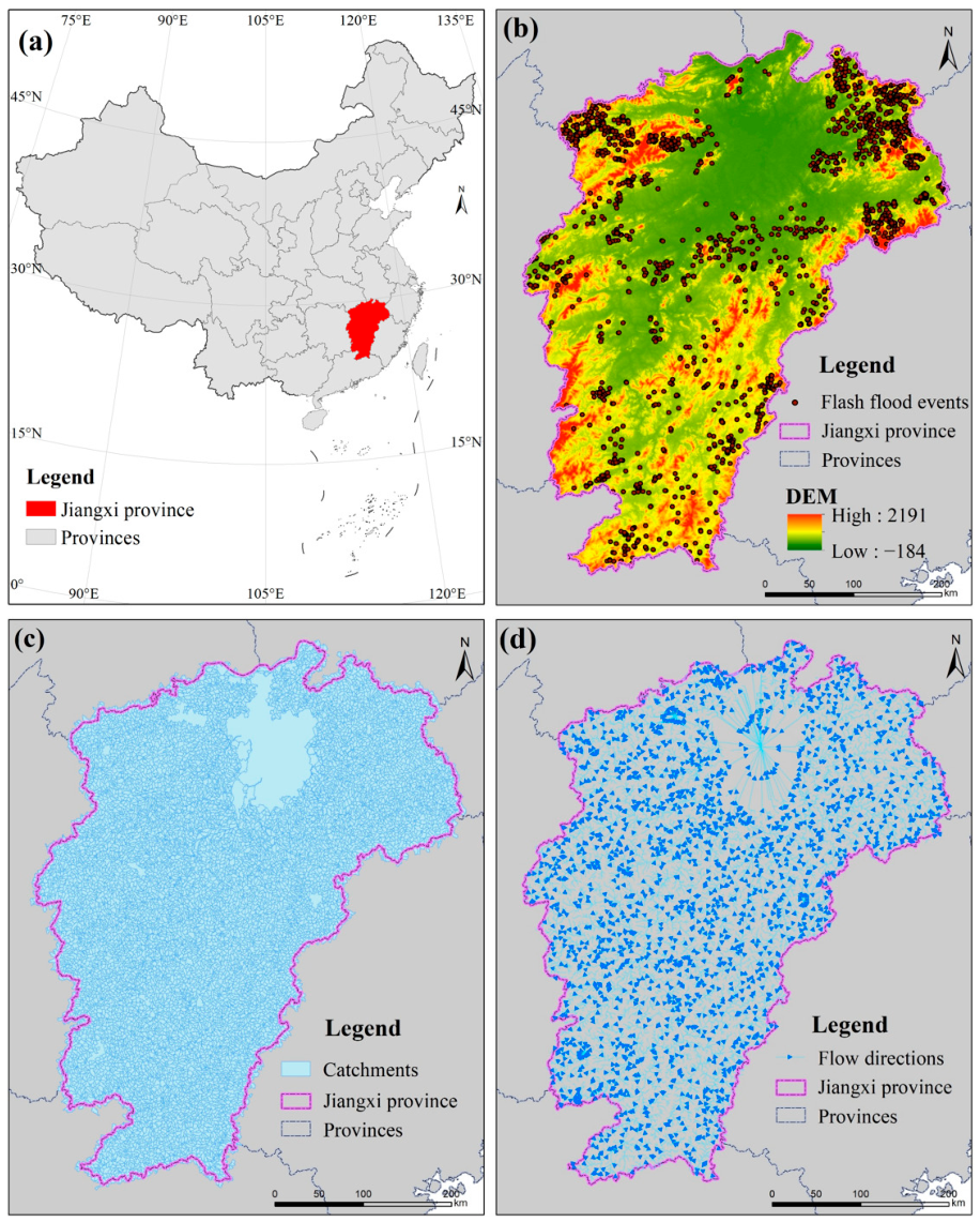
The study area is Jiangxi province, China. It covers an area of approximately 166,900 km² and extends from 113°34′ E to 118°28′ E longitude and 24°29′ N to 30°04′ N latitude, as shown in Figure 1a. It is a region dominated by mountains and hills that comprise approximately 78% of its terrain [51], as shown in Figure 1. As one of China’s wettest provinces, Jiangxi receives between 1341 and 1943 mm of annual precipitation. This rainfall is unevenly distributed; it is heavier in the south and east than in the north and west, with 42–53% falling between April and June. The province’s centripetal drainage system converges on Poyang Lake through a dense river network. Driven primarily by seasonal rainfall, river runoff peaks in the summer, with 53–60% of the annual total flowing between April and June. This combination of steep terrain, a dense hydrographic network, and concentrated rainfall results in rapid water convergence and high hydrological sensitivity in small catchments. Consequently, Jiangxi is highly susceptible to flash floods. Between 1950 and 2015, flash floods affected nearly 800,000 people and caused almost 2000 deaths [5,15], posing a persistent challenge for flash flood prevention and mitigation [52].

2.2. Materials

This study utilized three datasets for flash flood regionalization: catchments, flash flood factors, and historical flash flood events.

2.2.1. Catchments and Their Flow Directions

Catchments can effectively represent the spatial processes of flash flood formation, runoff convergence, and propagation, so we chose catchments as the basic units for flash flood regionalization. The catchments and their flow directions in Jiangxi province were derived from the 30 m ASTER GDEM. Hydrological and topographic analysis tools in ArcGIS 10.8 were first employed to generate a preliminary delineation of catchments and their flow directions [9]. Following previous studies [5,9], to ensure the representativeness and stability of the basic units, catchments with excessively small areas (i.e., less than 10 km²) were merged into adjacent ones. Ultimately, 12,245 valid catchments were obtained, with areas ranging from 10 to 50 km². The catchments and their corresponding flow directions are presented in Figure 1c and Figure 1d, respectively. To obtain flash flood features for each catchment, the zonal statistics tool in ArcMap 10.8 was used to extract catchment-level flash flood features.

2.2.2. Flash Flood Factors

To characterize the flash flood hazard, flash flood factors are selected based on two main aspects: meteorological factors and underlying surface factors [3,7,8,9]. Meteorological factors such as short-duration rainfall represent the directed factors that trigger or amplify flash flood events, while underlying factors such as topography and vegetation reflect the geographical environment conditions on which flash flood occurrences depend. Note that the selected flash flood factors should comprehensively reflect the physical processes associated with flash flood occurrence.

(1)

Meteorological factors

Rainfall is a critical meteorological factor in triggering flash floods [7,8], as short-duration high-intensity precipitation can rapidly increase surface runoff, while prolonged rainfall can also lead to soil saturation, decrease water storage capacity, and further enhance surface runoff, increasing flash flood risk. To characterize these effects, the maximum rainfall over different time intervals (1 h, 3 h, and 6 h) and annual exceedance probabilities (1%, 2%, 5%, 20%, and 50%) were selected as meteorological factors for catchment-based flash flood regionalization. Twenty-two rainfall factors were chosen as meteorological conditions for flash floods, as shown in

Table 1. Meteorological factors.

Time Interval	Annual Exceedance Probability (AEP)	Rainfall Factors and Descriptions
1 h, 3 h, and 6 h	1%, 2%, 5%, 20%, 50%	Maximum 1 h, 3 h, and 6 h rainfall corresponding to 1%, 2%, 5%, 20%, and 50% AEP
1 h, 3 h, 6 h, 12 h, and 24 h	-	Annual average maximum 1 h, 3 h, 6 h, 12 h and 24 h rainfall (2008–2018)
Year	-	Annual average rainfall and annual average number of rainstorm days

.

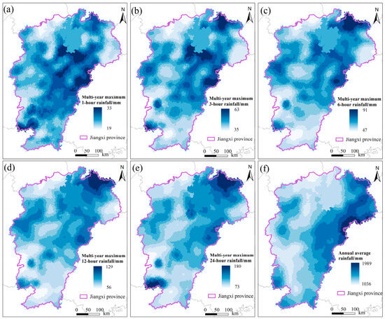
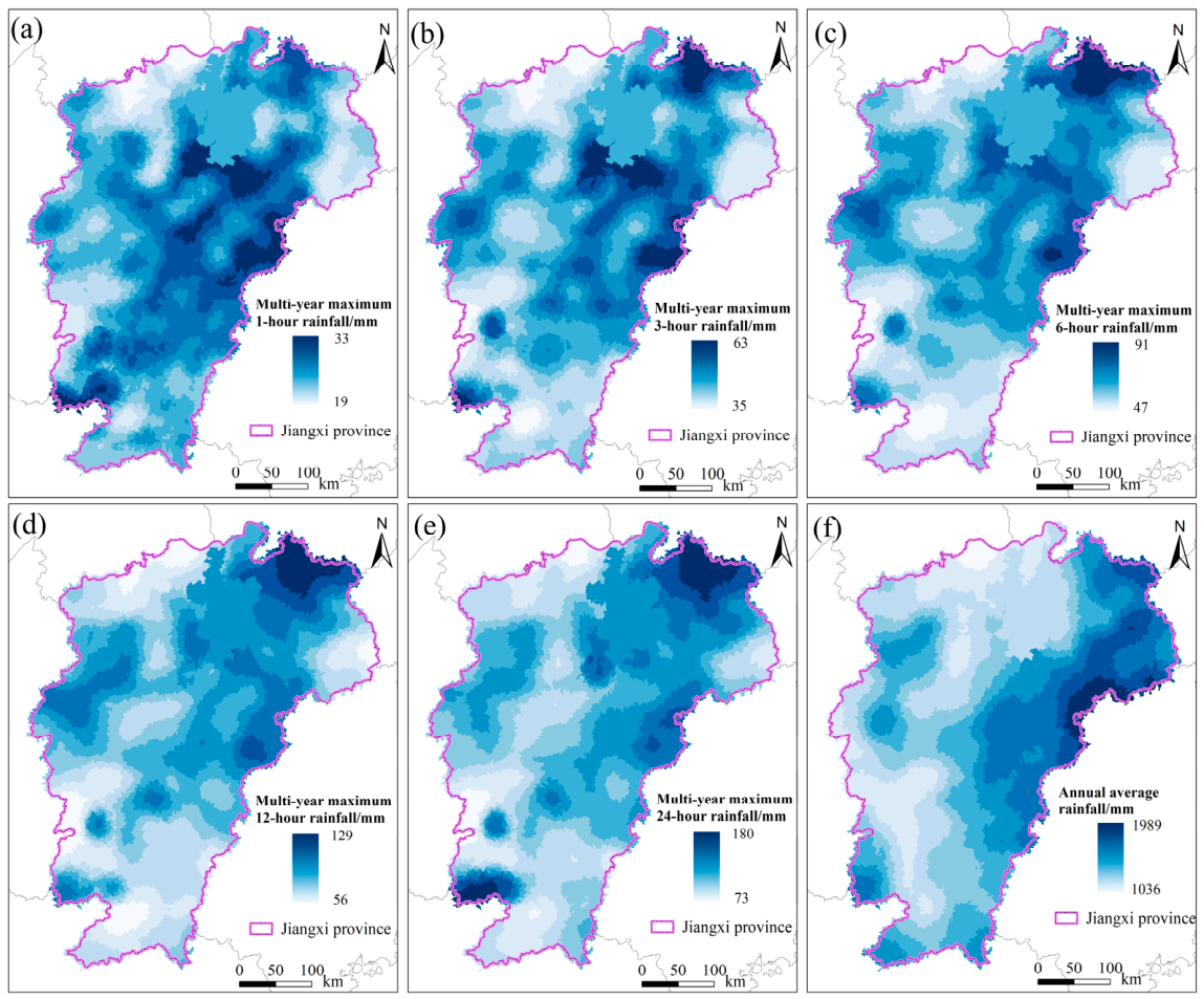
The original rainfall data were obtained from the Hourly Precipitation 0.1° Grid Dataset from the National Meteorological Information Center (https://data.cma.cn/), covering the period from 1 January 2008 to 31 December 2018. Using this gridded dataset, we first calculated and organized the rainfall data for each grid at various time intervals for each year. We then plotted the Pearson-III frequency curves based on empirical frequencies to estimate the statistical parameters of these curves by moments for curve fitting [53]. The fitted frequency curves were subsequently used to derive the maximum rainfall values at different time intervals (1 h, 3 h, and 6 h) and annual exceedance probabilities (1%, 2%, 5%, 20%, and 50%) on a 0.1° × 0.1° grid, yielding a total of twenty-two rainfall factors. Figure 2 shows six representative rainfall factors in Jiangxi province.

(2)

Underlying surface factors

The underlying surface of flash floods is largely shaped by topography and land surface conditions, which provide both the foundation and the predisposing factors for their occurrence [5,15,54,55]. Thus, the selected underlying surface factors influencing flash floods included the DEM, elevation difference, slope, normalized difference vegetation index (NDVI), height above the nearest drainage (HAND), surface roughness, and stable infiltration rate, as displayed in

Table 2. Underlying surface factors.

Underlying Surface Factors	Description
DEM	ASTER GDEM 30 m DEM
Elevation difference	Derived from 30 m DEM
Slope	Derived from 30 m DEM
NDVI	China Annual Vegetation Index Spatial Distribution Dataset in 2015
HAND	Global Hydrography Datasets
Surface roughness	Surface roughness coefficient for each land use type from the National Flash Flood Investigation and Evaluation Project (NFFIEP)
Stable infiltration rate	Saturation infiltration coefficients for soil types from NFFIEP

.

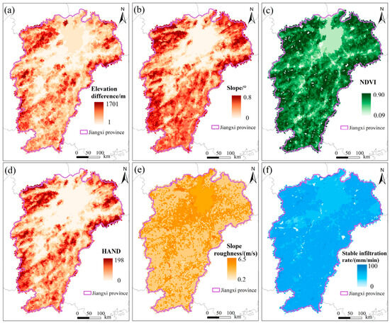
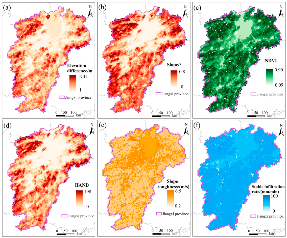
The DEM, elevation difference, and slope were selected as topographical factors. The DEM was obtained from the 30 m ASTER GDEM, from which both the elevation difference and slope were derived. The elevation difference and slope are displayed in Figure 3a and Figure 3b, respectively. NDVI, which reflects vegetation cover density, was obtained from the Annual Vegetation Index Dataset of China for 2015, as shown in Figure 3c. HAND, which normalizes elevation relative to drainage networks and represents soil gravity and local drainage potentials, was obtained from the Global Hydrography Datasets (https://hydro.iis.u-tokyo.ac.jp/~yamadai/MERIT_Hydro/, accessed on 1 January 2026), as shown in Figure 3d. Surface roughness, which affects the flow velocity of flash floods, was derived from land use data provided by NFFIEP [9] using roughness coefficients for different land use types from SCS (1986) [56], as shown in Figure 3e. Stable infiltration rate, which is the constant rate at which water can enter the soil profile, was estimated using soil type data provided by NFFIEP [9] and the saturation infiltration coefficients for various soil types from Li et al. [57], as shown in Figure 3f.

2.2.3. Historical Flash Flood Events Inventory

Historical flash flood events were utilized to evaluate the flash flood regionalization results. The historical flash flood events inventory was also obtained from NFFIEP [9], covering the period from 1950 to 2015. In NFFIEP, flash flood events were identified based on comprehensive post-event investigations conducted by local water resources authorities, integrating information from disaster yearbooks, statistical reports, field surveys, and hydrological analyses [9]. The spatial distribution of historical flash flood events is shown in Figure 1b, indicating that most events occurred in the mountainous and hilly areas of northwestern, northeastern, and southern Jiangxi province. Notably, historical flash flood events were not incorporated into the training procedure for the clustering models; instead, they were only employed as an independent reference data to evaluate the performance of the final regionalization maps.

2.3. Methodology

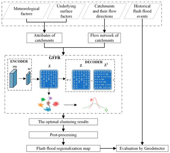
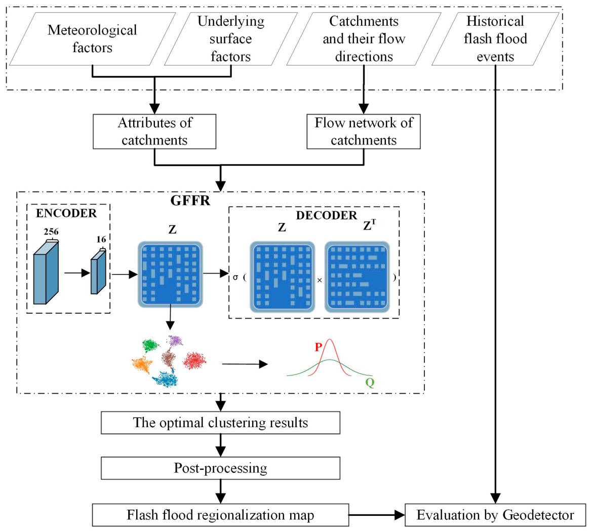
The proposed GFFR focuses on enhancing the latent representations of catchment attributes and their spatial structure (e.g., topology and flow directions) using GCNNs. Catchments, the basic spatial units for clustering, are abstracted as a directed graph to characterize their spatial structure, while meteorological and underlying factors associated with flash floods are used as node attributes for GFFR. GFFR is applied in Jiangxi province, China and compared with three existing widely used clustering methods (i.e., K-means, SKATER, and DAEGC) to demonstrate its effectiveness. The flowchart of this study is shown in Figure 4 and it involves six main steps.

(1)

Data preparation. Prepare data for flash flood regionalization, including catchments and their flow directions, meteorological factors, underlying surface factors, and historical flash flood events.

(2)

Data preprocessing. Preprocess the catchment-level meteorological and underlying surface factors as catchment attributes, and construct a directed graph using these attributes and flow directions.

(3)

Model construction and training. Build and train the GFFR on the directed graph to generate clustering results for flash floods in Jiangxi province using a predefined number of clusters. Inspired by the graph clustering [58], the GFFR inherits the widely used architecture of deep graph clustering models and consists of two main modules, an encoder module and a decoder module, as illustrated in Figure 4.

(4)

Cluster optimization. Calculate the clustering validity indexes to determine the optimal number of clusters.

(5)

Post-processing. Refine the optimal clustering results to produce the final flash flood regionalization map for Jiangxi province, China.

(6)

Evaluation and analysis. Assess the regionalization results by applying the Geodector method to the historical flash flood events [59].

2.3.1. Construction of the Directed Graph

Based on flow direction relationships among catchments, which is calculated by the D8 algorithm on the DEM, each catchment was linked to its directly downstream neighboring catchment, thereby constructing a directed graph which represents the catchments’ network structure. It should be noted that this graph construction relies on physically meaningful upstream–downstream relationships among catchments, so spatially connected catchments are required. In this directed graph, nodes represent individual catchments, flash flood features of catchments were served as the node attributes, and edges indicate the flow direction from upstream to downstream. The corresponding adjacency matrix $A$ was defined as follows:

$$A_{ij}=\left\{\begin{array}{c}1, if catchment i directly flows into catchment j \\ 0, otherwise\end{array}\right.$$

(1)

where $A_{ij}=1$ indicates catchment $i$ directly flows into catchment $j$. This adjacency matrix effectively characterizes the hydrological network topography and serves as the structural input of the proposed GFFR method.

2.3.2. Proposed GFFR Method

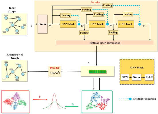
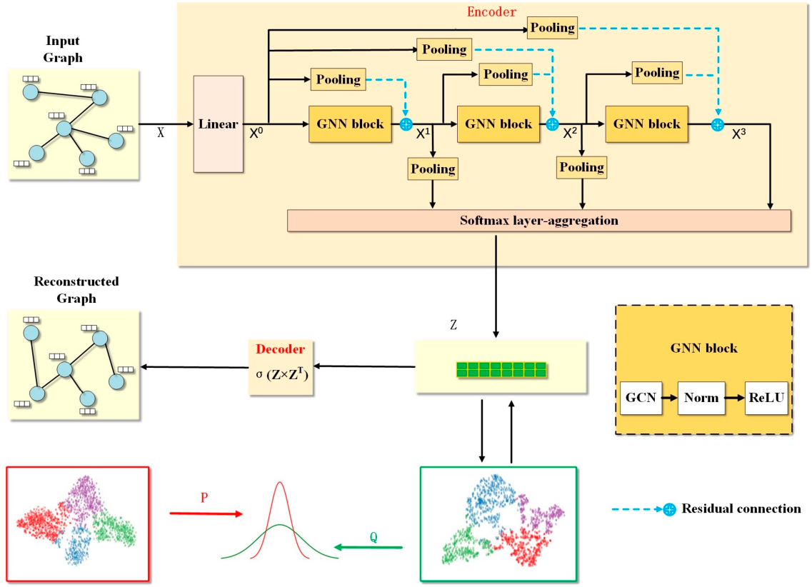
Inspired by a state-of-the-art graph clustering neural network of Deep Attentional Embedding Graph Clustering (DAEGC) [58], GFFR is enhanced using graph convolutional network (GCN) layers and residual connections. With the abstractly directed graph of catchments for flash floods, the proposed GFFR follows the typical structure of GCNNs and consists of two main modules: the encoder and the decoder [38,39,43,45,47,60]. Inspired by the graph clustering [58,61], the architecture of GFFR is designed in Figure 5.

(1)

The encoder module

The encoder module in GFFR is designed to realize the latent representation of nodes in the graph, as displayed in Figure 5. It primarily consists of three graph neural network (GNN) blocks. Initially, a linear layer reduces the high-dimensional input $X$ to $X^0$ during the encoding process. Subsequently, $X^l$ from each layer is passed sequentially through the GNN block, which includes a GCN layer, a Normalization layer, and the ReLU function. The GCN layers can effectively capture both node attributes and the structural information within a graph, enabling the encoder to extract the latent representation of the nodes in GFFR [62]. The GCN layers transform the input attributes $X^l$ into a new representation $X^{l+1}$ by propagating and aggregating information from neighboring nodes:

$$ReLU\left(x\right)=\left\{\begin{array}{c}x,x\ge 0\\ 0,x<0\end{array}\right.,$$

(2)

$$X^{l+1}=ReLU\left({\tilde{D}}^{-{\displaystyle \frac{1}{2}}}\tilde{A}{\tilde{D}}^{-{\displaystyle \frac{1}{2}}}{X}^l{w}^l\right),$$

(3)

$$\tilde{A}=A+I,$$

(4)

$${\tilde{D}}_{ii}={\sum }_j{\tilde{A}}_{ij},$$

(5)

where $X^l$ denotes the input of the $l$th layer in Equation (3), $\tilde{A}$ is the sum of adjacency matrix $A$ defined in Equation (1) and identity matrix $I$ in Equation (4), $\tilde{D}$ denotes the degree matrix of the adjacent matrix in Equation (5), and $w^l$ denotes the trainable linear transformation weight matrix for layer $l$.

The mean pooling operation is used to solve the dimension inconsistency across layers, while the residual connections between GNN blocks, which is proposed in ResNet, are introduced to avoid gradient-related and over-smoothing issues. Finally, inspired by Chi, Wang, Hao and Xia [61], a softmax layer aggregation is applied to the outputs of GNN blocks, and the final latent representation $Z$ of the directed graph, which jointly encodes the node attributes $X$ and structural information $A$, is calculated by weighted sum for the decoder of GFFR in Equations (6) and (7).

$$X^l=GNN\left(X^{l-1},A\right)+\alpha X^0+\beta X^{l-1},$$

(6)

$$Z={\displaystyle \sum _{l=1}^L}{softmax(W}^l)X^l$$

(7)

where $W^l$($l=1,\dots ,L$) denotes the learnable weight of layer $l$ in Equation (7), $X^l$ denotes the output for layer $l$ in Equation (7), $X^0$ denotes the original input of the directed graph of catchments, and $\alpha$ and $\beta$ are residual connection hyperparameters.

(2)

The decoder module

The decoder module aims to execute both graph reconstruction and graph clustering using the node representations generated by the encoder module. For graph reconstruction, an inner-product decoder in Equation (8) is utilized to predict the inter-node connections within the graph. The reconstruction error is then calculated by the reconstruction loss function $L_r$ in Equation (9).

$${\widehat{A}}_{ij}=sigmoid\left(Z_i^T{Z}_j\right),$$

(8)

$$L_r={\displaystyle \sum _{i=1}^n}BCE(A_{ij},{\widehat{A}}_{ij})$$

(9)

where $Z_i$ denotes the feature of node $i$, ${\widehat{A}}_{ij}$ is the probability of the presence of an edge between reconstructed nodes $i$ and $j$, $A_{ij}$ is the value between nodes $i$ and $j$ in the adjacent matrix of the original directed graph of catchments, and BCE(·) denotes the binary cross entropy loss function.

For graph clustering, the t-distribution, a heavy-tailed distribution widely used for similarity modeling in representation learning [58], is first used as a soft clustering assignment function to define the clustering probability distribution $Q=q_{iu}$, which maps the distance between node feature $z_i$ and the centroid of cluster ${\mu }_u$ into a similarity score, thereby facilitating graph clustering-oriented feature learning and representation. To emphasize higher probability distributions, the square of $q_{iu}$ is used to define the target distribution $P=p_{iu}$. Finally, the Kullback–Leibler (KL) divergence between distributions $P$ and $Q$ is calculated to quantify the graph clustering error, which is represented by the clustering loss function $L_c$ in Equation (10).

$$L_c=KL(P||Q)={\sum }_i{\sum }_u{p}_{iu}log{\displaystyle \frac{p_{iu}}{q_{iu}}},$$

(10)

To enhance the performance of both graph reconstruction and clustering, a joint loss function $L$ is formulated by combining the errors from graph reconstruction and self-optimal graph clustering in Equation (11).

$$L=L_r+\gamma L_c{Z}^T,$$

(11)

where $L_r$ and $L_c$ respectively denote the error function of the graph reconstruction and the graph clustering, and $\gamma$ is the balance coefficient.

The clustering results of GFFR, which simultaneously considers both the attribute and structure of catchments for flash flood regionalization, can be achieved through joint training that combines graph reconstruction and graph clustering.

(3)

Model implementation

The proposed GFFR model was implemented in python using PyTorch 1.9.0 deep learning framework. In the GFFR, following previous empirical studies [37,45,58,63] and after multiple rounds of experimental tuning, the dimensions of three GCN layers were set to 512, 256, and 128, respectively. The residual connection hyperparameters $\alpha$ and $\beta$ were set to 0.2 and 0.5, respectively [61]. The balance coefficient $\gamma$ in the loss function was set to 10 after parameter sensitivity analysis in Section 4.1. The GFFR model was trained for 50 epochs with a learning rate of 0.001 using the Adam optimizer.

To validate the performance of the proposed GFFR method, two typical traditional clustering algorithms (K-means and SKATER) and a graph clustering neural network (DAEGC) were selected for comparison.

2.3.3. Determining the Optimal Number of Clusters

The predefined number of clusters can significantly influence the results of clustering methods. Therefore, it is crucial to identify the best number of clusters to avoid over-dispersed or over-concentrated clustering results. Based on several experiments, the cluster number is set from 2 to 10 for K-means, DAEGC, and GFFR, while it ranges from 2 to 20 for SKATER. Two clustering validity indexes—Clustering Quality Index (CQI) [5] and Calinski–Harabasz Index (CHI) [64]—were selected to determine the optimal number of clusters. CQI evaluates the similarity of catchment attributes; a lower CQI value reflects stronger internal homogeneity within clusters and thus better clustering quality [5]. CHI measures the ratio of inter-cluster dispersion to intra-cluster dispersion; a higher CHI value indicates that inter-cluster differences are much large than intra-cluster differences, corresponding to better clustering quality [64]. Therefore, the clustering result with the lower CQI and higher CHI can be viewed as the optimal result.

2.3.4. Post-Processing

The initial clustering results of K-means, Ward and GFFR often contain several spatially non-adjacent clusters (i.e., multi-polygons), while each region in regionalization maps is typically treated as a spatially contiguous polygon [5,15,16,17]. Therefore, post-processing is necessary to enforce spatial contiguity, in which isolated small polygons are merged into adjacent large ones to obtain non-overlapping and relatively large regions [5]. To ensure the area balance of the regions after merging, the coefficient of variation (CV) of each region’s area and the first-order difference (FOD) of CV were calculated to determine the merge endpoint. For SKATER, it is already considered spatial contiguity during clustering, so no additional post-processing is required.

2.3.5. Evaluation Method for Regionalization Results

Geodetector 0.2.1 is a spatial analysis tool for revealing general patterns of inequitable spatial distributions [59]. If a response variable significantly impacts an explanatory variable, their spatial distributions are expected to show similarity [65]. The factor detector of Geodetector is commonly used to assess the relative importance of independent variables to dependent variables [5,66]. Therefore, the factor detector is employed to evaluate the distribution consistency of the historical flash flood events with flash flood regionalization results. Inspired by previous studies [5,67,68], the Getis-Ord Gi* statistic is first applied to generate the high or low values cluster (i.e., density) of flash flood events, which is used as the response variable in Geodetector. Then, the regions from the flash flood regionalization results are regarded as the explanatory variable to calculate the q-statistic by Geodetector, which evaluates the homogeneity of the historical flash flood event density within these regions. A higher q-statistic indicates strong spatial consistency and thus better regionalization performance.

3. Results

3.1. Optimal Number of Clusters

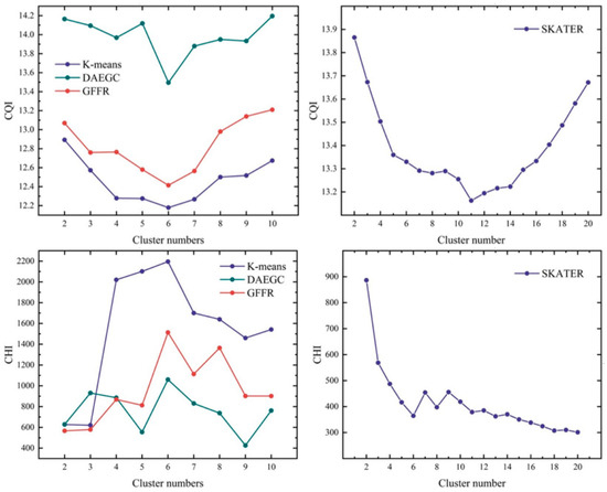
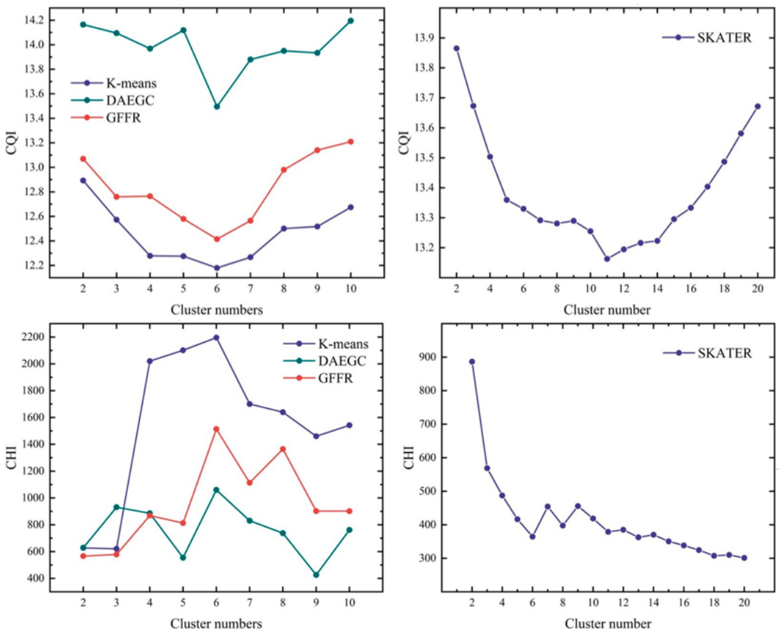
To determine the optimal number of clusters for each method, the CQI and CHI values for all four methods (i.e., K-means, SKATER, DAEGC, and GFFR) with varying numbers of clusters are calculated in Figure 6. These results indicate that, for all methods, CQI values initially decrease and then increase as the number of clusters rises, whereas CHI values exhibit the opposite trend. This pattern suggests that increasing the number of clusters initially reduces differences among catchments within each region, leading to a decrease in CQI and an increase in CHI. However, when the number of clusters becomes too large, differences among catchments increase, resulting in higher CQI values and lower CHI values. For K-means, CQI decreases from 12.89 to a minimum value of 12.18 and then increases to 12.66, while CHI increases from 612 to a maximum value of 2192 before declining to 1534. For SKATER, CQI gradually decreases from 13.87 to a minimum value of 13.16 and then increases to 13.67, whereas CHI continuously decreases from 887 to 301. DAEGC exhibits the highest CQI values among all methods, ranging from 13.49 to 14.18, and its CHI values vary between 424 and 1057. For GFFR, CQI ranges from 12.41 to 13.21, while CHI increases from 563 to a maximum value of 1508 and then gradually decreases. Specifically, for K-means, DAEGC, and GFFR, the minimum CQI and maximum CHI occur at six clusters. The minimum CQI are 12.18, 13.49, and 12.41, respectively, while the corresponding maximum CHI values are 2192, 1057, and 1508, indicating that six clusters are the optimal number for the three methods. For SKATER, the minimum CQI occurs at eleven clusters with a value of 13.16, while CHI favors fewer clusters. Despite this, eleven clusters are selected as the optimal number for SKATER, as they better capture the diversity within the data.

3.2. Clustering Results of Flash Floods

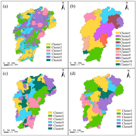
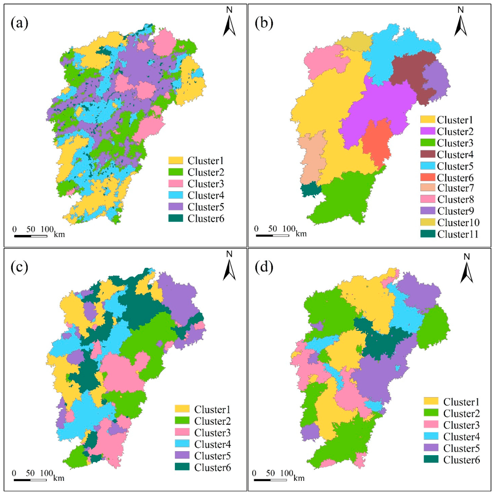
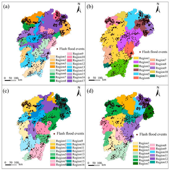
Figure 7 displays the flash flood clustering results obtained using the four methods with their respective optimal number of clusters. All methods produced a combination of large and small clusters, indicating that post-processing is required to convert the clustering results into regionalization maps. Among them, as shown in

Table 3. The number of isolated polygons and compactness for each method.

Method	Number of Isolated Polygons	Maximum Compactness	Minimum Compactness	Average Compactness
K-means	656	0.913	0.013	0.481
SKATER	0	0.912	0.052	0.606
DAEGC	158	0.914	0.198	0.697
GFFR	42	0.914	0.265	0.742

, K-means yielded the most fragmented pattern, with the largest number of small isolated polygons (656) and the lowest average compactness (0.481), indicating highly dispersed and irregular regions. SKATER, constrained by spatial contiguity, generated the fewest spatially separated clusters among the four methods, and achieved a relatively higher average compactness (0.606). DAEGC also generated many small isolated clusters (158) embedded within large ones and further improved average compactness to 0.697, resulting in fragmented and less uncompacted regions. In contrast, GFFR produced only 42 small isolated polygons, and the identified clusters were more compact (average compactness = 0.742) than those obtained by the other three methods.

3.3. Regionalization Maps of Flash Floods

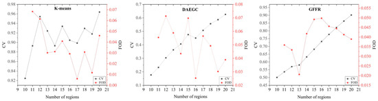
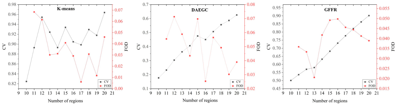
As shown in Figure 8, as the number of regions decreases during the post-processing merging procedure, the FOD for K-means, DAEGC, and GFFR initially decreases, indicating that smaller or isolated patches are being merged. This confirms the validity and necessity of merging small patches. The FOD for K-means, DAEGC, and GFFR reaches a minimum when the number of regions is 17 (FOD = 0.031), 16 (FOD = 0.032), and 13 (FOD = 0.021), respectively. Afterward, the FOD increases, and the CV accelerates as more small patches are merged. Therefore, the optimal number of regions is set to 17, 16, and 13 for K-means, DAEGC, and GFFR, respectively.

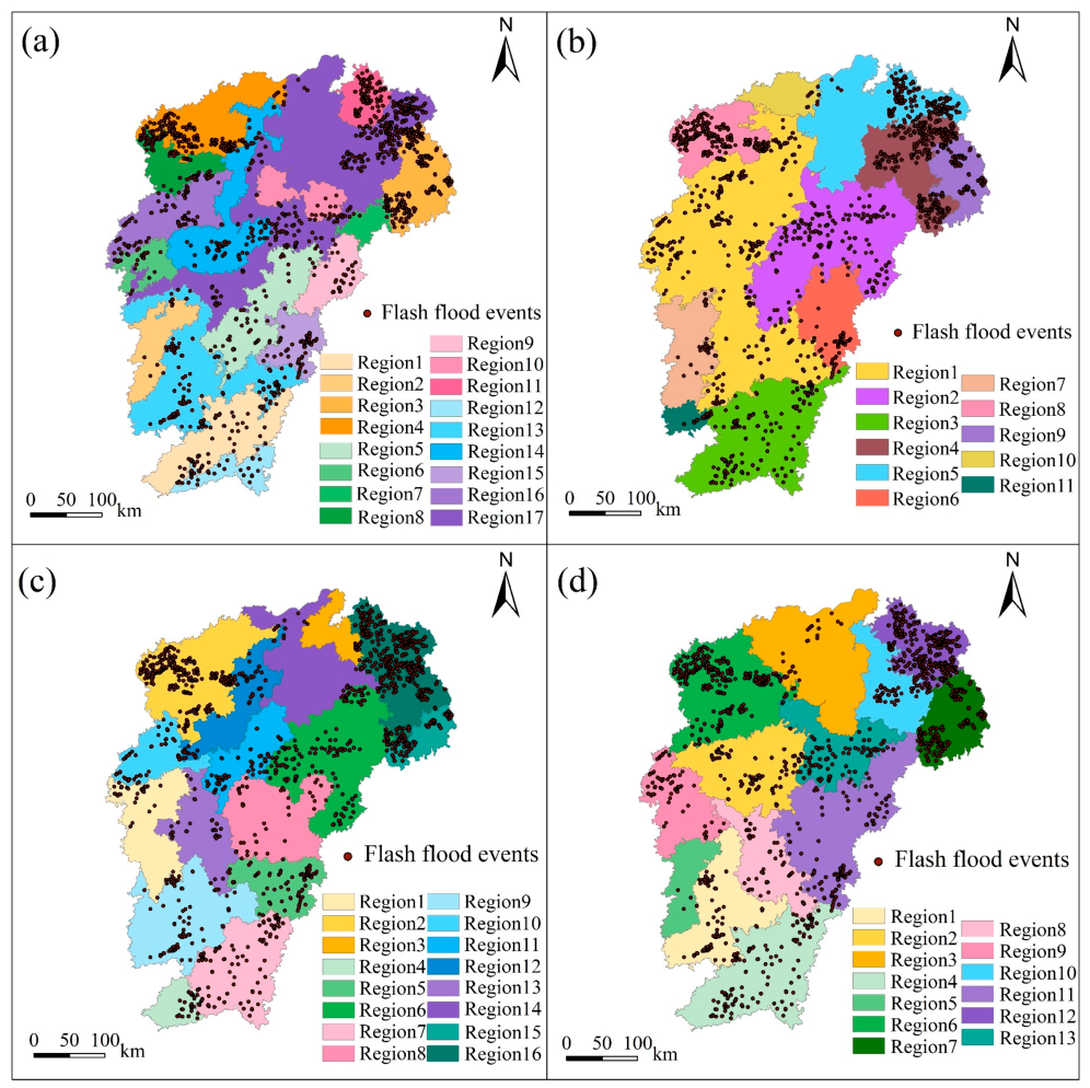
After post-processing, the flash flood regionalization maps generated by the four methods are shown in Figure 9. The K-means-based regionalization map shows several regions that are either elongated or contain disjointed (island) polygons, such as Region14 and Region17. This is primarily because K-means only considers the attribute similarity of catchments (i.e., meteorological and underlying surface factors) and ignores their spatial structure, resulting in geographically fragmented regions. In contrast, the SKATER method yields a regionalization map without island polygons. However, it includes several large and elongated regions (e.g., Region1). Although SKATER incorporates spatial contiguity, it relies solely on the original spatial relationships and fails to adapt to newly formed neighborhood structures during clustering. As a result, it can produce regions with significant variation in area. Similarly, the DAEGC-based regionalization map does not produce island polygons but includes multiple elongated regions, such as Region12 and Region14, while extremely uneven region sizes often indicate spatial fragmentation or over-aggregation, both of which reduce the interpretability and reliability of regionalization results. Among the four methods, the GFFR approach produces the most compact and spatially coherent regions, with no island polygons and relatively balanced area sizes. GFFR effectively delineates catchments with similar attributes and spatial structures into homogenous regions, providing more rational regionalization for flash floods. For example, in the GFFR map, flash flood events in the northwest area near Jiuling Mountain are clearly divided into Region6, while flash flood events in the northeast are grouped into Region7 (low-density events) and Region12 (high-density events).

3.4. Evaluation of Flash Flood Regionalization Maps

In traditional regionalization studies, the homogeneity of delineated regions has typically been assessed by cluster validity metrics due to the absence of ground truth data. However, these regions were often derived from post-processing clustering results, which failed to directly evaluate the spatial consistency of actual flash flood events. Thus, the Geodetector was leveraged to quantitatively evaluate the homogeneity of historical flash flood event density within the identified regions. The q-statistics of the regionalization maps produced by K-means, SKATER, DAEGC, and GFFR are 0.406, 0.516, 0.792, and 0.81, respectively. These results indicate substantial differences in the determinant power of each method in capturing the spatial distribution of flash flood events. Specifically, the q-statistic of GFFR is 0.404, 0.294, and 0.018 higher than that of K-means, SKATER, and DAEGC, respectively. This provides quantitative evidence that the GFFR method more effectively explains the spatial heterogeneity of flash flood events and achieves higher regional homogeneity than the other three methods.

4. Discussion

4.1. Parameter Sensitivity Analysis

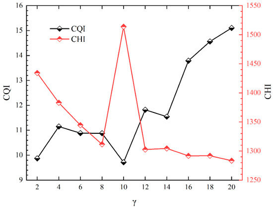
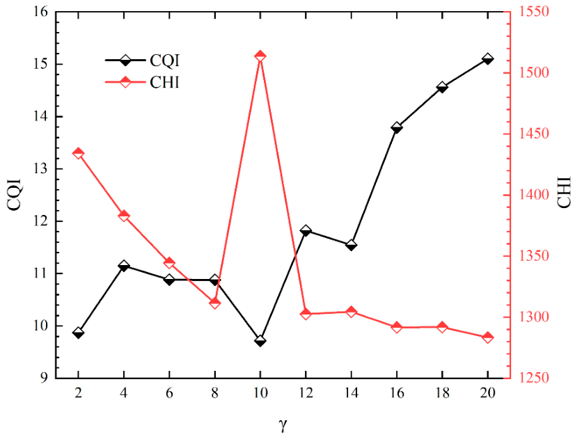
According to Equation (11), the overall loss function of GFFR consists of graph reconstruction loss and graph clustering loss, where hyperparameter $\gamma$ controls the relative contribution of these two terms. To assess the impact of the hyperparameter $\gamma$ in the loss function on the performance of GFFR, a parameter sensitivity analysis was conducted. The $\gamma$ value was varied from 2 to 20 in increments of 2, and the corresponding CQI and CHI metrics were computed for each $\gamma$ value. As illustrated in Figure 10, the model achieved the optimal performance at $\gamma$ = 10, with the lowest CQI and the highest CHI. Therefore, the hyperparameter γ in the loss function was set to 10 in the proposed GFFR for flash flood regionalization.

4.2. Ablation Analysis

The proposed GFFR model was developed by enhancing the baseline DAEGC through three key modifications. First, the graph attention network (GAT) layers in DAEGC were replaced with GCN layers to improve feature aggregation and better capture structural information. Second, the residual connections (RC) were integrated in GFFR to mitigate gradient-related and over-smoothing issues. Lastly, a directed graph was built to more accurately represent the spatial structure and hierarchy of catchments. To evaluate these improvements, we conducted an ablation analysis by comparing configurations with and without GCN layers, residual connections, and the directed graph of catchments [69], as shown in

Table 4. Ablation results of GFFR.

	CQI	CHI
GFFR + Undirected graph	11.888	622.389
Baseline + GAT	11.073	1094.364
Baseline + GAT + RC	10.588	816.028
Baseline + GCN	10.526	882.647
Baseline + GCN + RC (GFFR)	9.715	1513.771

. All experiments reported in Table 3 were conducted using six clusters, which correspond to the optimal number of clusters for GFFR, following Section 3.1, and with loss function hyperparameter $\gamma$ set to 10, following Section 4.1, and other training parameters follow Section 2.3.2. The directed graph implementation significantly outperformed the undirected counterpart, as evidenced by lower CQI and higher CHI values in the second and last rows of Table 4. For instance, the directed graph configuration led to an 18.28% reduction in CQI compared to the undirected graph. GCN layers also achieved superior performances to GAT layers, reducing CQI by 4.94% while increasing CHI by 19.34%. The inclusion of residual connections further enhanced clustering performances by decreasing CQI and increasing CHI. Overall, the ablation results collectively demonstrate that the integration of GCN layers, residual connections, and the directed graph of catchments critically enhanced the performance of GFFR for flash flood regionalization.

4.3. Limitation and Future Work

Traditional regionalization methods primarily focus on the attribute similarity of spatial units when delineating homogeneous regions, often ignoring the spatial structure similarity. The proposed GFFR leverages advanced GCNN techniques in deep learning to simultaneously integrate both the attribute and spatial structure of catchments, allowing for more accurate delineation of homogeneous regions for flash floods. In contrast to existing regionalization methods, the GCNN used in GFFR eliminates the need for selecting key factors [5,9], as it can directly learn the latent representation of both attribute and spatial structure. Despite the merits, this study has several limitations. First, the evaluation of regionalization performance mainly relied on historical events, which are insufficient to capture the changing features of flash floods under future conditions driven by climate change and human disturbances (e.g., alterations in underlying face properties and mitigation measures). In this context, the regionalization map derived by GFFR may have uncertainties when applied to future flash flood prevention. Furthermore, the key objective of GFFR is to acquire more accurate delineations of homogenous regions, so as to provide more basis for subsequent hydrological modeling and region-specific mitigation strategies, rather than directly generating forecasts. Therefore, integrating GFFR with forecasting models is required to further improve the overall ability for flash flood prevention and management.

While GFFR has so far only been applied in Jiangxi province, China, future work could further investigate its transferability in other study areas for different categories of flash floods by fine-tuning the model parameters (e.g., the number of hidden layers, the number of nodes in the hidden layers, and the coefficient $\gamma$ in the loss function). Additionally, although this study mainly focuses on flash floods, GFFR may also hold the potential for delineating homogeneous regions based on both attribute and structure similarities in other types of floods or geographical domains, such as climate, ecology and hydrology [24,27,29,70].

5. Conclusions

This paper proposed a new graph-clustering-neural-network-based flash flood regionalization method (GFFR) to obtain flash flood regionalization map. The method employed a graph clustering neural network to simultaneously account for both attribute and structure similarities in partitioning homogeneous regions. The architecture of GFFR was designed to incorporate an encoder, decoder, GCN layers, residual connections, and the directed graph of catchments. Taking Jiangxi province, China, as the case study area, meteorological and underlying surface factors of catchments were collected as the attribute, and flow directions between catchments were used to construct a directed graph representing the spatial structure. With the directed graph as input, GFFR was trained to generate clustering results, which are then post-processed into the final flash flood regionalization map with thirteen homogeneous regions in Jiangxi province. The flash flood regionalization map of GFFR achieved a determinant power of 81% for the spatial distribution of historical flash flood events, which is 24% higher than the average performance of the three existing typical clustering methods of K-means, SKATER, and DAEGC. Therefore, the proposed GFFR offers a promising option for regionalization in flash floods and can be applied to other geoscience fields.

References

- Keefer, D.K.; Wilson, R.C.; Mark, R.K.; Brabb, E.E.; Brown, W.M.; Ellen, S.D.; Harp, E.L.; Wieczorek, G.F.; Alger, C.S.; Zatkin, R.S. Real-time landslide warning during heavy rainfall. Science 1987, 238, 921–925. [Google Scholar] [CrossRef] [Scilit]
- Liu, J.; Xiong, J.; Chen, Y.; Sun, H.; Zhao, X.; Tu, F.; Gu, Y. An integrated model chain for future flood risk prediction under land-use changes. J. Environ. Manag. 2023, 342, 118125. [Google Scholar] [CrossRef] [Scilit]
- Yao, J.; Zhang, X.; Luo, W.; Liu, C.; Ren, L. Applications of stacking/blending ensemble learning approaches for evaluating flash flood susceptibility. Int. J. Appl. Earth Obs. Geoinf. 2022, 112, 102932. [Google Scholar] [CrossRef] [Scilit]
- Duan, H.; Cao, Z.; Luo, J.; Shen, M. Ai-driven opportunities and challenges in lake remote sensing. Inf. Geogr. 2025, 1, 100014. [Google Scholar] [CrossRef] [Scilit]
- Zhang, R.; Chen, Y.; Zhang, X.; Ma, Q.; Ren, L. Mapping homogeneous regions for flash floods using machine learning: A case study in jiangxi province, China. Int. J. Appl. Earth Obs. Geoinf. 2022, 108, 102717. [Google Scholar] [CrossRef] [Scilit]
- Liu, Y.; Huang, Y. Why flash floods occur differently across regions? A spatial analysis of China. Water 2020, 12, 3344. [Google Scholar] [CrossRef] [Scilit]
- Ma, M.; Zhao, G.; He, B.; Li, Q.; Dong, H.; Wang, S.; Wang, Z. Xgboost-based method for flash flood risk assessment. J. Hydrol. 2021, 598, 126382. [Google Scholar] [CrossRef] [Scilit]
- Garambois, P.A.; Roux, H.; Larnier, K.; Labat, D.; Dartus, D. Parameter regionalization for a process-oriented distributed model dedicated to flash floods. J. Hydrol. 2015, 525, 383–399. [Google Scholar] [CrossRef] [Scilit]
- Liu, C.; Ma, Q.; Zhang, X.; Li, C.; Li, Q.; Gourbesville, P.; Guo, L.; Ding, L. Identification and quantitative analysis of flash flood risks for small catchments in China: A new operational modelling approach. LHB 2022, 108, 2019561. [Google Scholar] [CrossRef] [Scilit]
- Beck, H.E.; van Dijk, A.I.J.M.; de Roo, A.; Miralles, D.G.; McVicar, T.R.; Schellekens, J.; Bruijnzeel, L.A. Global-scale regionalization of hydrologic model parameters. Water Resour. Res. 2016, 52, 3599–3622. [Google Scholar] [CrossRef] [Scilit]
- Ma, M.; Liu, C.; Zhao, G.; Xie, H.; Jia, P.; Wang, D.; Wang, H.; Hong, Y. Flash flood risk analysis based on machine learning techniques in the Yunnan province, China. Remote Sens. 2019, 11, 170. [Google Scholar] [CrossRef] [Scilit]
- Xiong, J.; Li, J.; Cheng, W.; Wang, N.; Guo, L. A gis-based support vector machine model for flash flood vulnerability assessment and mapping in China. ISPRS Int. J. Geo-Inf. 2019, 8, 297. [Google Scholar] [CrossRef] [Scilit]
- Ahmed, A.; Rahman, A.; Rafi, R.S.M.H.; Khan, Z.; Mannan, H. Statistical and physical significance of homogeneous regions in regional flood frequency analysis. Water 2025, 17, 1799. [Google Scholar] [CrossRef] [Scilit]
- Arseni, M.; Rosu, A.; Calmuc, M.; Calmuc, V.A.; Iticescu, C.; Georgescu, L.P. Development of flood risk and hazard maps for the lower course of the Siret River, Romania. Sustainability 2020, 12, 6588. [Google Scholar] [CrossRef] [Scilit]
- Wang, N.; Lombardo, L.; Tonini, M.; Cheng, W.; Guo, L.; Xiong, J. Spatiotemporal clustering of flash floods in a changing climate (China, 1950–2015). Nat. Hazards Earth Syst. Sci. 2021, 21, 2109–2124. [Google Scholar] [CrossRef] [Scilit]
- Cutter, S.L.; Golledge, R.; Graf, W.L. The big questions in geography. Prof. Geogr. 2002, 54, 305–317. [Google Scholar] [CrossRef] [Scilit]
- Aydin, O.; Janikas, M.V.; Assunção, R.M.; Lee, T.-H. A quantitative comparison of regionalization methods. Int. J. Geogr. Inf. Sci. 2021, 35, 2287–2315. [Google Scholar] [CrossRef] [Scilit]
- Tobler, W.R. A computer movie simulating urban growth in the Detroit region. Econ. Geogr. 1970, 46, 234–240. [Google Scholar] [CrossRef] [Scilit]
- Goodchild, M.F. The validity and usefulness of laws in geographic information science and geography. Ann. Assoc. Am. Geogr. 2004, 94, 300–303. [Google Scholar] [CrossRef] [Scilit]
- Zhu, A.X.; Lu, G.; Liu, J.; Qin, C.Z.; Zhou, C. Spatial prediction based on third law of geography. Ann. GIS 2018, 24, 225–240. [Google Scholar] [CrossRef] [Scilit]
- Song, Y. The second dimension of spatial association. Int. J. Appl. Earth Obs. Geoinf. 2022, 111, 102834. [Google Scholar] [CrossRef] [Scilit]
- Song, Y. Geographically optimal similarity. Math. Geosci. 2022, 55, 295–320. [Google Scholar] [CrossRef] [Scilit]
- Zhang, H.; Zhou, X.; Yang, Y.; Wang, H.; Ye, X.; Tang, G. Advancing process-oriented geographical regionalization model. Ann. Am. Assoc. Geogr. 2024, 114, 2388–2413. [Google Scholar] [CrossRef] [Scilit]
- Peel, M.C.; Finlayson, B.L.; McMahon, T.A. Updated world map of the köppen-geiger climate classification. Hydrol. Earth Syst. Sci. 2007, 11, 1633–1644. [Google Scholar] [CrossRef] [Scilit]
- Huang, X.; Liu, A.; Li, J. Mapping and analyzing the local climate zones in China’s 32 major cities using landsat imagery based on a novel convolutional neural network. Geo-Spat. Inf. Sci. 2021, 24, 528–557. [Google Scholar] [CrossRef] [Scilit]
- Bailey, R.G. Identifying ecoregion boundaries. Environ. Manag. 2004, 34, S14–S26. [Google Scholar] [CrossRef] [Scilit]
- Kearney, S.; Coops, N.; Stenhouse, G.; Nelson, T. Ecoanthromes of Alberta: An example of disturbance-informed ecological regionalization using remote sensing. J. Environ. Manag. 2019, 234, 297–310. [Google Scholar] [CrossRef] [Scilit]
- Agarwal, A.; Maheswaran, R.; Sehgal, V.; Khosa, R.; Sivakumar, B.; Bernhofer, C. Hydrologic regionalization using wavelet-based multiscale entropy method. J. Hydrol. 2016, 538, 22–32. [Google Scholar] [CrossRef] [Scilit]
- Nadoushani, S.; Dehghanian, N.; Saghafian, B. A fuzzy hybrid clustering method for identifying hydrologic homogeneous regions. J. Hydroinform. 2018, 20, 1367–1386. [Google Scholar] [CrossRef] [Scilit]
- Khajehei, S.; Ahmadalipour, A.; Shao, W.; Moradkhani, H. A place-based assessment of flash flood hazard and vulnerability in the contiguous United States. Sci. Rep. 2020, 10, 448. [Google Scholar] [CrossRef] [Scilit] [PubMed]
- Arganis, M.; Preciado, M.; Luna, F.D.; Cruz, L.; Domínguez, R.; Santana, O. Application of a regionalization method for estimating flash floods: Cuautepec basin, Mexico. Water 2023, 15, 303. [Google Scholar] [CrossRef] [Scilit]
- Duque, J.C.; Ramos, R.; Suriñach, J. Supervised regionalization methods: A survey. Int. Reg. Sci. Rev. 2007, 30, 195–220. [Google Scholar] [CrossRef] [Scilit]
- Roushangar, K.; Alizadeh, F. A multiscale spatio-temporal framework to regionalize annual precipitation using k-means and self-organizing map technique. J. Mt. Sci. 2018, 15, 1481–1497. [Google Scholar] [CrossRef] [Scilit]
- Ley, R.; Casper, M.C.; Hellebrand, H.; Merz, R. Catchment classification by runoff behaviour with self-organizing maps (som). Hydrol. Earth Syst. Sci. 2011, 15, 2947–2962. [Google Scholar] [CrossRef] [Scilit]
- Assunção, R.M.; Neves, M.C.; Câmara, G.; da Costa Freitas, C. Efficient regionalization techniques for socio-economic geographical units using minimum spanning trees. Int. J. Geogr. Inf. Sci. 2006, 20, 797–811. [Google Scholar] [CrossRef] [Scilit]
- Middleton, R.S. Geographical Distillation: Application of the p-Median, Traveling Salesman, and Regionalization Problems. Ph.D. Thesis, University of California, Santa Barbara, CA, USA, 2006. [Google Scholar]
- Lim, K.-L.; Jiang, X.; Yi, C. Deep clustering with variational autoencoder. IEEE Signal Process. Lett. 2020, 27, 231–235. [Google Scholar] [CrossRef] [Scilit]
- Wu, Z.; Pan, S.; Chen, F.; Long, G.; Zhang, C.; Philip, S.Y. A comprehensive survey on graph neural networks. IEEE Trans. Neural Netw. Learn. Syst. 2020, 32, 4–24. [Google Scholar] [CrossRef] [Scilit]
- Zhang, H.; Li, P.; Zhang, R.; Li, X. Embedding graph auto-encoder for graph clustering. IEEE Trans. Neural Netw. Learn. Syst. 2022, 34, 9352–9362. [Google Scholar] [CrossRef] [Scilit]
- Chen, Y.; Zhou, J.; Ge, Y.; Dong, J. Uncovering the rapid expansion of photovoltaic power plants in China from 2010 to 2022 using satellite data and deep learning. Remote Sens. Environ. 2024, 305, 114100. [Google Scholar] [CrossRef] [Scilit]
- Tsitsulin, A.; Palowitch, J.; Perozzi, B.; Müller, E. Graph clustering with graph neural networks. J. Mach. Learn. Res. 2023, 24, 1–21. [Google Scholar] [CrossRef] [Scilit]
- Chen, Y.; Zhou, J.; Xu, C.; Ma, Q.; Zhang, X.; Zhou, Y.; Ge, Y. Structure-aware deep learning network for building height estimation. Int. J. Appl. Earth Obs. Geoinf. 2025, 137, 104443. [Google Scholar] [CrossRef] [Scilit]
- Tian, F.; Gao, B.; Cui, Q.; Chen, E.; Liu, T.-Y. Learning deep representations for graph clustering. In Proceedings of the AAAI Conference on Artificial Intelligence; AAAI: Washington, DC, USA, 2014. [Google Scholar]
- Zhou, J.; Cui, G.; Hu, S.; Zhang, Z.; Yang, C.; Liu, Z.; Wang, L.; Li, C.; Sun, M. Graph neural networks: A review of methods and applications. AI Open 2020, 1, 57–81. [Google Scholar] [CrossRef] [Scilit]
- Li, X.; Hu, Y.; Sun, Y.; Hu, J.; Zhang, J.; Qu, M. A deep graph structured clustering network. IEEE Access 2020, 8, 161727–161738. [Google Scholar] [CrossRef] [Scilit]
- Peng, Z.; Liu, H.; Jia, Y.; Hou, J. Attention-driven graph clustering network. In Proceedings of the 29th ACM International Conference on Multimedia; ACM: New York, NY, USA, 2021; pp. 935–943. [Google Scholar]
- Tu, W.; Zhou, S.; Liu, X.; Guo, X.; Cai, Z.; Cheng, J. Deep fusion clustering network. arXiv 2020, arXiv:2012.09600. [Google Scholar]
- Yao, S.; Huang, B. Spatiotemporal interpolation using graph neural network. Ann. Am. Assoc. Geogr. 2023, 113, 1856–1877. [Google Scholar] [CrossRef] [Scilit]
- Zhu, D.; Zhang, F.; Wang, S.; Wang, Y.; Cheng, X.; Huang, Z.; Liu, Y. Understanding place characteristics in geographic contexts through graph convolutional neural networks. Ann. Am. Assoc. Geogr. 2020, 110, 408–420. [Google Scholar] [CrossRef] [Scilit]
- Li, Y.; Zhang, C.; Cui, P.; Hassan, M.; Duan, Z.; Bhattacharyya, S.; Yao, S.; Zhao, Y. Flash flood regionalization for the Hengduan mountains region, China, combining gnn and shap methods. Remote Sens. 2025, 17, 946. [Google Scholar] [CrossRef] [Scilit]
- Chen, Y.; Xu, C.; Ge, Y.; Zhang, X.; Zhou, Y.N. A 100 m gridded population dataset of China’s seventh census using ensemble learning and big geospatial data. Earth Syst. Sci. Data 2024, 16, 3705–3718. [Google Scholar] [CrossRef] [Scilit]
- Liu, S.; Feng, L.; Xie, J.; Ke, Y. Assessing urban flood resilience with unascertained measurement theory: A case study of Jiangxi province, China. Sustainability 2026, 18, 49. [Google Scholar] [CrossRef] [Scilit]
- Izinyon, O.; Ihimekpen, N.; Igbinoba, G. Flood frequency analysis of Ikpoba River catchment at Benin City using log Pearson type iii distribution. J. Emerg. Trends Eng. Appl. Sci. 2011, 2, 50–55. [Google Scholar]
- Liu, J.; Xiong, J.; Chen, Y.; Sun, H.; Zhao, X.; Tu, F.; Gu, Y. A new avenue to improve the performance of integrated modeling for flash flood susceptibility assessment: Applying cluster algorithms. Ecol. Indic. 2023, 146, 109785. [Google Scholar] [CrossRef] [Scilit]
- Zhang, M.; Zhang, D.; Jin, Y.; Wan, X.; Ge, Y. Evolution of soil moisture mapping from statistical models to integrated mechanistic and geoscience-aware approaches. Inf. Geogr. 2025, 1, 100005. [Google Scholar] [CrossRef] [Scilit]
- Cronshey, R. Urban Hydrology for Small Watersheds; US Department of Agriculture, Soil Conservation Service, Engineering Division: Washington, DC, USA, 1986.
- Li, X.; Chang, S.X.; Salifu, K.F. Soil texture and layering effects on water and salt dynamics in the presence of a water table: A review. Environ. Rev. 2014, 22, 41–50. [Google Scholar] [CrossRef] [Scilit]
- Wang, C.; Pan, S.; Hu, R.; Long, G.; Jiang, J.; Zhang, C. Attributed graph clustering: A deep attentional embedding approach. arXiv 2019, arXiv:1906.06532. [Google Scholar]
- Wang, J.F.; Li, X.H.; Christakos, G.; Liao, Y.L.; Zhang, T.; Gu, X.; Zheng, X.Y. Geographical detectors-based health risk assessment and its application in the neural tube defects study of the Heshun region, China. Int. J. Geogr. Inf. Sci. 2010, 24, 107–127. [Google Scholar] [CrossRef] [Scilit]
- Liu, Y.; Xia, J.; Zhou, S.; Yang, X.; Liang, K.; Fan, C.; Zhuang, Y.; Li, S.Z.; Liu, X.; He, K. A survey of deep graph clustering: Taxonomy, challenge, application, and open resource. arXiv 2022, arXiv:2211.12875. [Google Scholar]
- Chi, H.; Wang, Y.; Hao, Q.; Xia, H. Residual network and embedding usage: New tricks of node classification with graph convolutional networks. J. Phys. Conf. Ser. 2022, 2171, 012011. [Google Scholar] [CrossRef] [Scilit]
- Kipf, T.N.; Welling, M. Semi-supervised classification with graph convolutional networks. arXiv 2016, arXiv:1609.02907. [Google Scholar]
- Bo, D.; Wang, X.; Shi, C.; Zhu, M.; Lu, E.; Cui, P. Structural deep clustering network. In Proceedings of The Web Conference 2020; ACM: New York, NY, USA, 2020; pp. 1400–1410. [Google Scholar]
- Caliński, T.; Harabasz, J. A dendrite method for cluster analysis. Commun. Stat. 1974, 3, 1–27. [Google Scholar] [CrossRef] [Scilit]
- Song, Y.; Wang, J.; Ge, Y.; Xu, C. An optimal parameters-based geographical detector model enhances geographic characteristics of explanatory variables for spatial heterogeneity analysis: Cases with different types of spatial data. GISci. Remote Sens. 2020, 57, 593–610. [Google Scholar] [CrossRef] [Scilit]
- Yang, L.; Li, X.; Yang, Q.; Zhang, L.; Zhang, S.; Wu, S.; Zhou, C. Extracting knowledge from legacy maps to delineate eco-geographical regions. Int. J. Geogr. Inf. Sci. 2021, 35, 250–272. [Google Scholar]
- Cao, Y.; Jia, H.; Xiong, J.; Cheng, W.; Li, K.; Pang, Q.; Yong, Z. Flash flood susceptibility assessment based on geodetector, certainty factor, and logistic regression analyses in Fujian province, China. ISPRS Int. J. Geo-Inf. 2020, 9, 748. [Google Scholar] [CrossRef] [Scilit]
- Liu, Y.; Yang, Z.; Huang, Y.; Liu, C. Spatiotemporal evolution and driving factors of China’s flash flood disasters since 1949. Sci. China Earth Sci. 2018, 61, 1804–1817. [Google Scholar] [CrossRef] [Scilit]
- Randall, N.; Heisenberg, G.; Duval, J.L.R. Generating aerial flood prediction imagery with generative adversarial networks. In Proceedings of the 17th International Joint Conference on Knowledge Discovery, Knowledge Engineering and Knowledge Management—KDIR; SciTePress: Setúbal, Portugal, 2025; pp. 15–27. [Google Scholar] [CrossRef] [Scilit]
- Zlati, M.L.; Antohi, V.-M.; Ionescu, R.-V.; Iticescu, C.; Georgescu, L.P. Quantyfing the impact of the water security index on socio-economic development in eu27. Socio-Econ. Plan. Sci. 2024, 93, 101912. [Google Scholar] [CrossRef] [Scilit]
Disclaimer/Publisher’s Note: The statements, opinions and data contained in all publications are solely those of the individual author(s) and contributor(s) and not of MDPI and/or the editor(s). MDPI and/or the editor(s) disclaim responsibility for any injury to people or property resulting from any ideas, methods, instructions or products referred to in the content. |
© 2026 by the authors. Licensee MDPI, Basel, Switzerland. This article is an open access article distributed under the terms and conditions of the Creative Commons Attribution (CC BY) license.