Fine-Grained Village Functional Differentiation in Rural Territorial Systems: A Few-Shot Hierarchical Graph Learning Approach

Abstract

Identifying village functional differentiation within rural territorial systems is essential for differentiated rural revitalization and place-based governance. However, existing approaches still lack effective analytical pathways for translating complex rural territorial relations and sparse planning labels into fine-grained measures of rural functional intensity. To address these gaps, this study develops a Few-Shot Hierarchical Graph Representation Learning (FH-GRL) framework. By integrating a Hierarchical Graph Infomax (HGI) model to capture cross-scale village–township–city relational dependencies and an Evidential Deep Learning (EDL) mechanism to map high-dimensional representations into class-specific evidence and Global Percentile Ranks (GPR), the framework supports fine-grained classification and continuous grading of rural functions. Empirical analysis in Pingdingshan City yields three main findings. First, within the present case study, FH-GRL shows more stable performance than traditional flat clustering and local graph models in identifying complex rural functions under limited labeled samples. Second, hierarchical context serves as a spatial calibration mechanism, reducing locally generated noise and improving the identification of village functional differentiation under spatial heterogeneity. Third, rural functional differentiation reflects the combined effects of place-based conditions and potential flow-related interaction conditions. In particular, Center villages show differentiated trajectories between endogenous production or service centers in agricultural plains and exogenous service centers along urban development axes. Overall, this study provides a planning-oriented quantitative framework for diagnosing rural functional differentiation under label scarcity and spatial heterogeneity. The GPR-based outputs can support the identification of high-intensity functional carriers, transitional villages, and general reserve areas, thereby providing diagnostic evidence for differentiated governance and tiered resource allocation. Rather than replacing formal planning judgment, the framework offers geospatially informed support for classified rural governance and more evidence-informed territorial planning.

1. Introduction

Rural territorial systems provide essential production, ecological, and cultural functions, and therefore remain central to contemporary rural transformation and governance [1,2,3]. However, rapid urbanization has intensified the spatial polarization of urban–rural factors, contributing to widespread rural decline [4,5,6]. Spatially, this systemic decline manifests across three main dimensions. In the production space, the fragmentation and abandonment of agricultural land have accelerated the weakening of agricultural functions [7,8]. In the living space, population loss and the increasing dispersion of rural settlements have raised infrastructure provision costs and reduced the efficiency of public services, thereby undermining the sustainability of rural living environments [9,10]. In the ecological space, disorderly development has increased pressure on natural and cultural landscapes and, in some cases, has led to irreversible degradation [11,12]. Because villages differ markedly in resource endowments, locational conditions, and developmental stages, “one-size-fits-all” planning often fails to support context-sensitive interventions, resulting in resource misallocation and governance inefficiency [13]. Accordingly, identifying village functional differentiation within rural territorial systems has become a prerequisite for differentiated governance and context-sensitive rural revitalization [14,15].

To better capture the complexity of rural territorial systems, village classification studies have increasingly developed multidimensional indicator systems integrating natural environmental and socioeconomic factors [16]. Existing approaches can be broadly divided into theory-driven deductive approaches and data-driven classification approaches. The former typically rely on expert knowledge or subjective weighting methods, such as the Analytic Hierarchy Process (AHP), and often struggle to maintain consistent evaluation standards across large and heterogeneous regions [17,18,19]. The latter seek to reduce subjective bias through objective weighting, dimensionality reduction, or unsupervised clustering, including methods such as Principal Component Analysis (PCA) and Self-Organizing Maps (SOM) [20,21,22,23,24]. Although both have contributed to village typology research, they remain limited in three important respects. First, many approaches focus primarily on village attributes themselves, while giving insufficient attention to the spatial relations, topological dependencies, and cross-scale interactions through which village functions are embedded in rural territorial systems [25,26,27,28]. Second, their applicability across large and heterogeneous regions remains weak, as models calibrated in one setting often perform poorly in areas with different geomorphological conditions, development contexts, and urban–rural linkages [29,30,31]. Third, many approaches still have difficulty translating classification outputs into governance-relevant planning semantics. Although village typologies are expected to inform practical village planning and rural spatial governance, data-driven categories may remain weakly connected to planning meanings, intervention priorities, and differentiated governance pathways if they are not interpreted within a policy-oriented territorial framework [20,32,33]. In practice, high-confidence village labels are difficult and costly to obtain because they often depend on statutory planning documents, expert knowledge, field investigation, and manual verification. Similar label-scarcity problems have also been widely recognized in geospatial classification tasks [34]. This makes village classification in many regions a label-scarce task, while also limiting the direct use of purely data-driven clusters in differentiated governance. Taken together, these limitations indicate that village classification should be understood not simply as the assignment of discrete labels, but as the identification of village functional differentiation within complex rural territorial systems.

In response to the pronounced heterogeneity of rural territorial systems, place-based governance has become an important principle in contemporary spatial governance [35,36,37,38]. Against this backdrop, China’s nationally promoted village classification framework provides a representative policy-oriented basis for the differentiated governance of complex rural territorial systems. At the national policy level, this framework generally distinguishes four main categories: agglomeration and upgrading villages, urban–suburban integration villages, characteristic protection villages, and relocation and consolidation villages [18,39,40]. Rather than constituting a simple list of village types, this framework captures the differentiated functional positioning of villages in terms of urban–rural linkages, network hierarchy, ecological constraints, and development potential. Urban–suburban integration villages are shaped primarily by exogenous urban spillovers and function as key nodes of factor exchange, reflecting the logic of urban–rural integration [41,42,43]. Agglomeration and upgrading villages with stronger service centrality and resource concentration act as local growth poles within township-level networks, highlighting their organizational and service functions [44,45,46]. Characteristic protection villages carry ecological and cultural missions, sustaining environmental security, human–nature interaction, and local cultural continuity [47]. Relocation and consolidation of villages reflect adaptive governance strategies under resource–environment constraints and differentiated development costs [48]. Taken together, these categories should not be viewed as rigid and mutually exclusive labels. Rather, they represent a multilevel functional organization logic linking village attributes, system-level positions, and governance orientations [49]. For analytical and modeling purposes, this study further refines the official characteristic protection category into Nature and Culture, and operationalizes the resulting analytical categories as Suburban, Center, Nature, Culture, and Relocate. Specifically, relocation, consolidation, and related governance-oriented interventions are interpreted along a shared intervention continuum and operationalized as Relocate.

Despite this policy-oriented conceptual foundation, clear analytical pathways for translating these policy logics into governance-relevant classification practice remain limited. A framework designed for this task should satisfy three core requirements. First, it should enable system-referenced relative evaluation, so that villages are assessed within the broader territorial system rather than in isolation, allowing relative resource advantages to be identified in complex contexts. Second, the framework needs to capture hierarchical interaction structures under different geographic conditions rather than treat villages as isolated units. This is necessary because villages are embedded in multilevel spatial relations that vary across mountainous areas, agricultural plains, and urban–rural transitional zones [50]. Third, village characteristics should be represented as continuous gradients instead of rigid labels, so that gradual differences in development potential and intervention priority can be identified more clearly across villages [51,52,53,54,55].

Given the pronounced networked and relational characteristics of rural territorial systems, graph representation learning (GRL) provides a promising paradigm for modeling non-Euclidean spatial relations in rural territorial systems [56]. By incorporating spatial adjacency, spillover effects, and local interactions through graph topology and message-passing mechanisms, GRL offers clear advantages for capturing spatial dependencies and relational structures in complex geographic settings [57,58]. Recent work on hierarchical graph models, especially in urban computing, also shows that multilevel graph learning can combine local semantics with broader structural context. HGI is one representative example of this line of work [59,60]. Yet direct transfer from urban settings to rural territorial systems is still difficult [41,50]. The difficulty lies not only in data form, but also in the way rural space is organized. In rural contexts, graph construction must deal with multidimensional areal units rather than point objects, which requires topology designed for contiguous village polygons [18,20,58]. Hierarchical aggregation must also reflect administrative nesting, functional differences, and uneven village roles within village–township–county systems instead of assuming equal node contributions [41,61,62]. In addition, reliable labels are usually sparse because they depend on planning documents, expert judgement, field investigation, and manual checking, a challenge also reflected in village-level identification and geospatial classification tasks [34,63]. Since few-shot learning is designed for tasks where only a small number of supervised samples are available, it provides a suitable strategy for this label-scarce classification setting [64]. Under these conditions, few-shot learning is not simply a technical option; it is closer to the actual data situation of village classification in large rural regions [20].

To respond to these constraints, this study develops a Few-Shot Hierarchical Graph Representation Learning (FH-GRL) framework for identifying fine-grained village functional differentiation in rural territorial systems. The framework links policy-oriented classification needs with algorithmic design. It first converts village observations into cross-scale networks based on multi-source geospatial data. It then applies HGI to learn representations that preserve local heterogeneity while incorporating broader hierarchical context. Finally, it introduces Evidential Deep Learning (EDL) and Global Percentile Rank (GPR) to move beyond discrete classification outputs and support continuous within-class differentiation of rural functions.

This study contributes in three related ways. First, it treats village classification as the identification of functional differentiation within a rural territorial system, so villages are interpreted in relation to multilevel spatial organization rather than as isolated units. Second, it provides an analytical route for linking village attributes, system-level positions, and within-class variation to governance-oriented classification. Third, it combines EDL and GPR to extend village identification from discrete category assignment to uncertainty-aware continuous differentiation in rural spatial planning.

The remainder of this paper is organized as follows. Section 2 and Section 3 describe the data foundation, indicator system, and methodological design of the FH-GRL framework. Section 4 presents the experimental results and comparative analyses. Section 5 discusses the main findings and their implications. Finally, Section 6 concludes the paper.

2. Study Area and Data

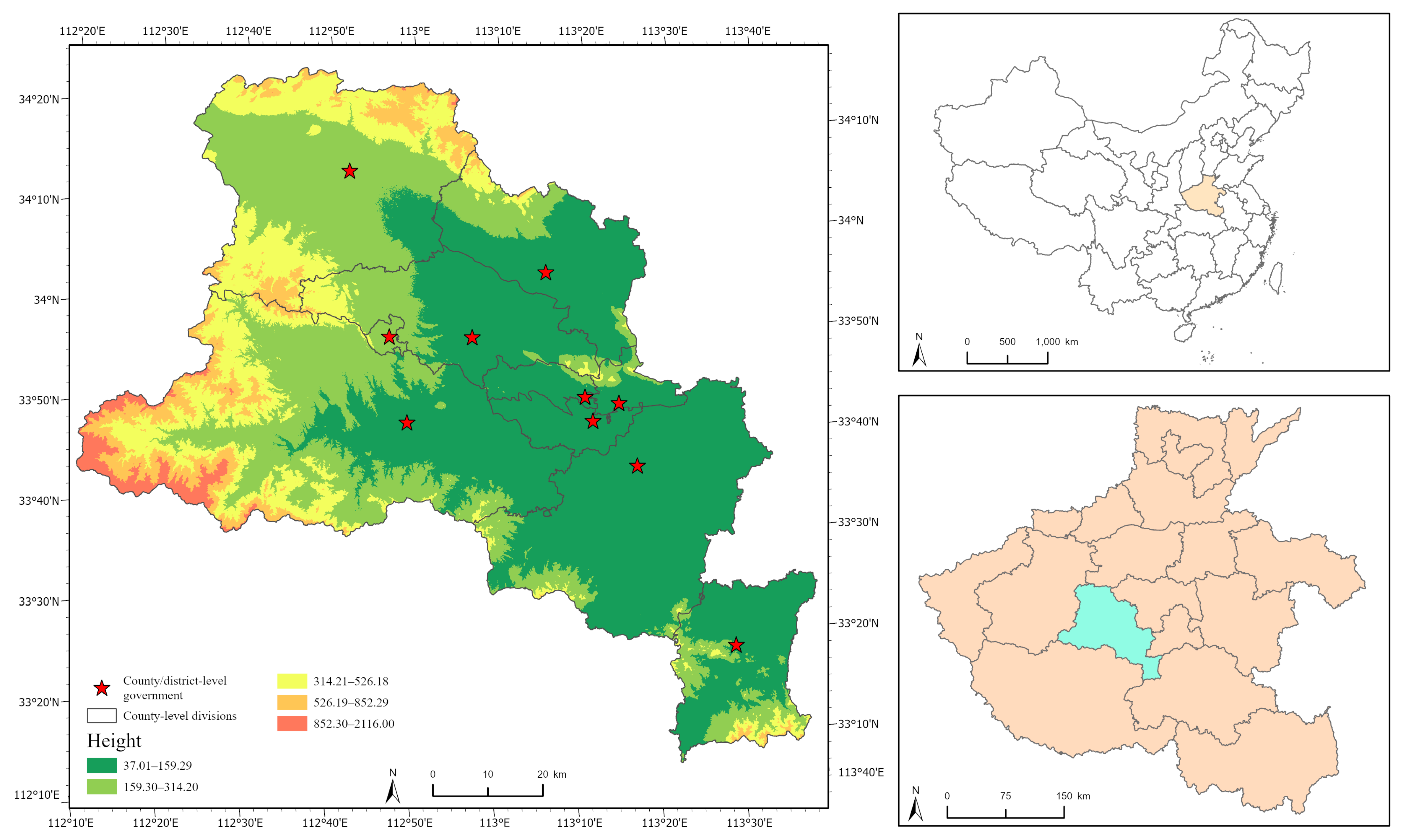
Pingdingshan City is located in central Henan Province, where resource-based industrial transition intersects with plain agricultural development. Administratively, the city includes four urban districts and six county-level divisions (Figure 1), with a resident population of about 4.88 million in 2020. As a coal-based resource city, Pingdingshan’s industrial development has long been shaped by coal mining and related heavy industries [65,66]. At the same time, agricultural production remains important, with local policy continuing to emphasize cultivated land protection, high-standard farmland construction, and stable grain production [67,68]. This mining–agricultural coexistence makes the study area suitable for examining village functional differentiation under the combined influence of industrial transition, agricultural production foundations, and rural revitalization.

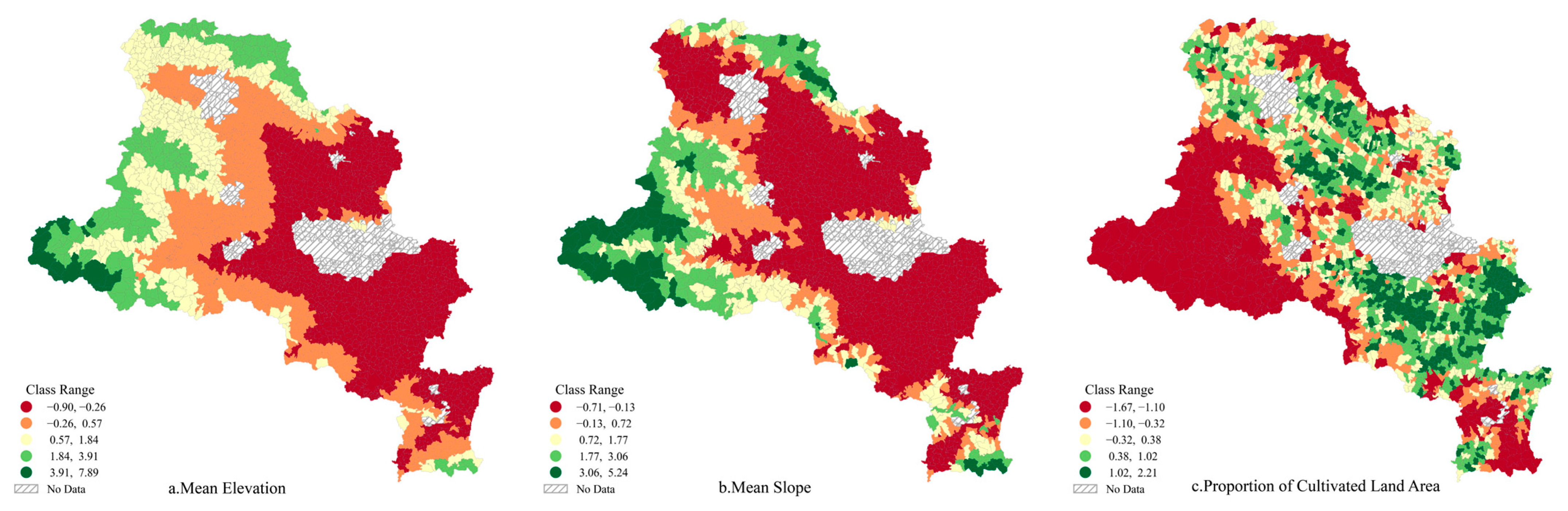
As shown in Figure 2, the study area has clear biophysical differences in both topography and cultivated land distribution. Mean elevation (Figure 2a) and slope (Figure 2b) form a strong spatial gradient, with higher terrain concentrated in the western and northeastern parts and lower terrain in the central, eastern, and southern parts. The proportion of cultivated land (Figure 2c) is higher in the central and southeastern plains, which are the main agricultural production areas, while mountainous areas with greater topographic relief generally contain less cultivated land. These patterns show a close relation between terrain conditions and land-use structure.

The study area also shows clear socioeconomic differences. The eastern plains have denser transport networks and a higher concentration of public service facilities, indicating stronger urban–rural linkages and factor flows. By contrast, the western mountainous areas are more constrained by topography and show lower transport accessibility and weaker facility provision. These spatial contrasts suggest that village functions are shaped by more than one type of condition. They depend on the combined effects of location, environment, resources, and development foundations. For this reason, a multidimensional indicator system is needed to describe village characteristics in an integrated way.

In defining the spatial analysis units, this study did not limit the sample to traditional administrative villages. Instead, it included all 2404 village-level territorial units within the township jurisdictions of the study area. Community-level units located along the fringes of built-up urban areas were also retained, because such fringe areas are commonly understood as peri-urban or urban–rural transitional interfaces where urban and rural land uses, settlements, and socioeconomic functions interact [69,70]. This treatment allows the sample to more fully cover the urban–rural continuum rather than imposing a strict urban–rural dichotomy. These units are contiguous polygons nested within township administrative boundaries, and they form the spatial basis for the multilevel graph structure used in the following analysis.

At the same time, labeled samples remain limited. Although the study area contains a large number of spatial units, only a small subset has explicit statutory planning labels in existing planning documents. This creates a sparse supervision setting for model training. In practical terms, it reflects a common few-shot condition in rural spatial planning: territorial coverage is broad, but high-confidence labeled samples are still scarce.

To describe the multidimensional characteristics of the rural territorial system and support the graph-based analysis, this study assembled data from three main sources: remote-sensing imagery, social sensing data, and basic geographic information. The remote-sensing data include annual maximum NDVI, ASTER GDEM, and nighttime light imagery, which were used to represent vegetation conditions, terrain, and nighttime development intensity. The social sensing data include POIs, gridded population data, and road network data, which were used to describe facility provision, population distribution, and transport connectivity. The basic geographic data include land survey data, administrative boundaries, and territorial spatial planning maps, which were used for boundary calibration, land-use verification, and the extraction of planning constraints. Detailed information on dataset names, spatial resolutions, years, and sources is reported in

Table 1. Summary of Multi-source Datasets.

Data Category	Dataset Name	Spatial Resolution/Scale	Year	Source and Description
Remote Sensing Imagery	Annual Maximum NDVI	30 m	2020	Derived on the Google Earth Engine (GEE) platform from remote-sensing imagery; processing informed by Yang et al. [71]
	ASTER GDEM V3	30 m	2020	NASA Earthdata; used to derive elevation and slope
	Cross-sensor Calibrated Monthly NTL Data	1 km	2020	Cross-sensor calibrated monthly nighttime light imagery, representing the stable nocturnal lighting and socioeconomic dynamics within the year. [72]
Social Sensing Data	Points of Interest (POIs)	–	2023	AutoNavi; includes 13 categories of facilities such as science and education, and medical services
	WorldPop	100 m	2020	WorldPop.org [73]; combined with township-level census statistics for constrained disaggregation
	Road Network Data	–	2023	OpenStreetMap (OSM); used to calculate road network density and accessibility
Basic Geographic Data	Third National Land Survey Data	Vector	2020	Natural resources authority; used for cultivated land area verification
	Administrative Boundary Data	Vector	2023	National Geomatics Center of China (NGCC)
	Territorial Spatial Planning Layers	Vector	2021–2035	Municipal Bureau of Natural Resources and Planning; used to extract planning constraint elements

.

During preprocessing, all raster and vector datasets were reprojected to the CGCS2000 coordinate system to ensure spatial alignment across different data sources. The year 2020 was set as the analytical benchmark for the experiment, and the biophysical, demographic, and land-use-related variables were constructed accordingly. The 2023 POI and road-network datasets were not used to represent an independent 2023 territorial structure, but were selected to better characterize the service, economic-activity, and accessibility conditions associated with the 2020 benchmark framework. This choice was based on a completeness comparison of online map records rather than a simple preference for more recent data. Specifically, POI and road-network datasets from the same months of 2020, 2021, 2022, and 2023 were compared with available 2020 township-level reference materials. Since these reference materials covered only selected townships rather than the entire study area, they were used only for coverage verification rather than as direct input data for model construction. The comparison showed that some facilities and road segments already existing around the benchmark period were not fully recorded in the 2020 online map datasets, indicating delayed updating and incomplete coverage of rural online map data. Among the four yearly datasets, the 2023 records provided the most complete coverage of the verified categories. Therefore, this study uniformly adopted the 2023 POI and road-network datasets to reduce underrepresentation caused by delayed online map updating. The detailed comparison is reported in Appendix A 

Table A2. Coverage comparison of POI and road-network records from 2020 to 2023.

Verified Category	Verified Reference Records in Selected Townships	Matched Records in 2020	Matched Records in 2021	Matched Records in 2022	Matched Records in 2023
Company and enterprise POIs	250	120	165	215	248
Accommodation and catering POIs	120	45	70	95	118
Living service POIs	185	80	115	150	185
Education service POIs	265	110	160	220	262
Medical service POIs	143	55	85	120	143
Government service POIs	210	95	140	185	208
Transportation service POIs	105	30	55	80	102
Road-network segments	233	100	155	195	233

Note: The reference records cover selected townships only and were used for coverage verification rather than as direct input data for model construction. Matched records refer to verified records identified in the online map datasets collected from the same months of 2020, 2021, 2022, and 2023.

.

3. Methodological Framework for Identifying Village Functional Differentiation

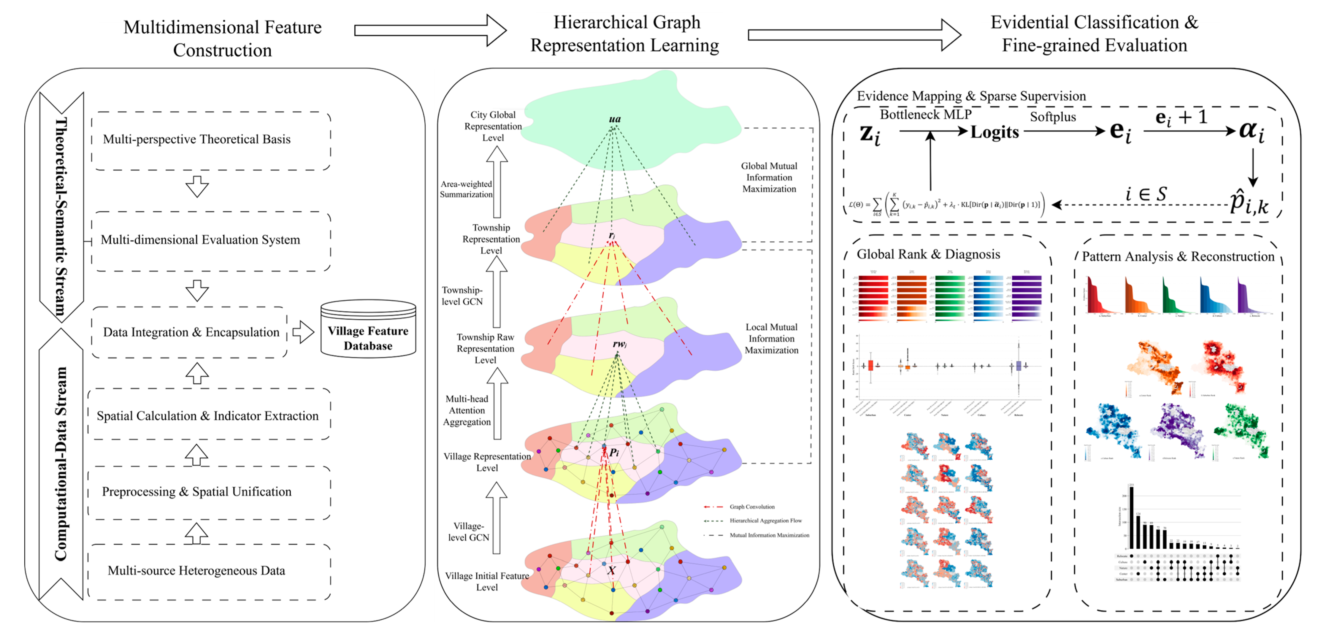
To transform multi-source heterogeneous spatial data into planning-oriented representations for fine-grained village functional differentiation, this study develops a FH-GRL framework. As shown in Figure 3, the framework can be understood as a three-stage planning-support workflow that links data construction, relational learning, and planning-oriented interpretation. First, multidimensional feature construction converts diverse village conditions—including locational accessibility, natural constraints, resource endowments, socioeconomic vitality, and public service provision—into a standardized feature matrix, enabling heterogeneous villages to be compared within a unified indicator space. Second, hierarchical graph representation learning embeds each village within a village–township–city topology, so that village functions are evaluated not as isolated local attributes but as outcomes shaped by cross-scale spatial relations and territorial context. Finally, under limited labeled samples, evidential classification and continuous evaluation map the learned representations into class probabilities, evidence scores, and GPR-based functional rankings, thereby supporting fine-grained classification, within-class differentiation, and planning-oriented prioritization. To improve readability while retaining reproducibility, the following subsections focus on the operational logic of each stage, whereas extended data-processing procedures, implementation settings, and validation materials are summarized in the appendices.

3.1. Multidimensional Feature Construction

To transform multi-source heterogeneous geospatial data into numerical features that can be processed by the graph learning framework, this section establishes a processing pipeline consisting of indicator selection, heterogeneous data quantification, and feature integration. Because a single observation dimension is insufficient to fully capture the coupled interactions among multiple elements within rural territorial systems, this study constructs an indicator system covering five dimensions: location and transportation, geographical environment, distinctive resources, socio-economic development, and infrastructure services. Based on this framework, 25 spatial indicators were selected (the theoretical dimensions and specific indicators are listed in

Table 2. Multidimensional Indicator System for Village Feature Construction.

Dimension	Influencing Factor	Operational Indicator
Location & Transportation	Urban Linkage	Euclidean Dist. to Central Urban Area Boundary
		Euclidean Dist. to County Seat
	Transport Network Connectivity	Density of Road Network
		Euclidean Dist. to Major Roads
	Macro-planning Guidance & Constraints	Location within Urban Dev. Axis/Node [Binary]
		Euclidean Dist. to Eco-Redline
Geographical Environment	Topographic Characteristics	Mean Slope
		Mean Elevation
	Ecological Baseline Condition	Mean NDVI
	Hydrological Condition	Euclidean Dist. to Major Water Systems
	Agricultural Production Resource	Proportion of Cultivated Land Area
Distinctive Resources	Agglomeration of High-level Tourism Resources	KDE of High-level Natural Landscapes
		KDE of High-level Cultural Landscapes
	Richness of Local Landscape	KDE of Local Natural Landscapes
		KDE of Local Cultural Landscapes
Socio-economic Development	Population Agglomeration Level	Resident Population Density
	Regional Economic Intensity	Mean Night-time Light Intensity
		Intra-annual Trend in Night-time Light Intensity
		KDE of Company & Enterprise POIs
	Commercial & Living Vitality	KDE of Accommodation & Catering POIs
		KDE of Living Service POIs
Infrastructure Services	Public Service Guarantee	KDE of Education Service POIs
		KDE of Medical Service POIs
	Administrative & Transport Efficiency	KDE of Government Service POIs
		KDE of Transportation Service POIs

, and detailed data sources and spatial calculation procedures are provided in Appendix A 

Table A1. Data Sources, Spatial Resolution, and Quantification Procedures for the Village-level Indicators.

Operational Indicator	Data Source & Dataset	Spatial Resolution/Format	Calculation Method & Processing Details
Euclidean Dist. to Central Urban Area/County Seat	Basic Geographic Information Data (Admin Boundaries & Govt. Seats)	Vector	Minimum Euclidean distance from the village polygon to the nearest boundary/seat.
Density of Road Network	OpenStreetMap (OSM) Road Network	Vector	Line density calculation within village polygons.
Euclidean Dist. to Major Roads	OpenStreetMap (OSM) Road Network	Vector	Minimum Euclidean distance from the village polygon to the nearest major road.
Location within Urban Dev. Axis/Node	Municipal/County Territorial Spatial Planning Layers	Vector	Spatial intersect; assigned binary values (1 if within axis/node, 0 otherwise).
Euclidean Dist. to Eco-Redline	Ecological Conservation Redline Data	Vector	Minimum Euclidean distance from the village polygon to the nearest redline boundary.
Mean Slope/Mean Elevation	ASTER GDEM V3	30 m Raster	Slope extraction followed by Zonal Statistics (Mean) within village boundaries.
Mean NDVI	Annual Maximum NDVI	30 m Raster	Zonal Statistics (Mean) within village boundaries.
Euclidean Dist. to Major Water Systems	Basic Geographic Information Data (Water Systems)	Vector	Minimum Euclidean distance from the village polygon to the nearest water system.
Proportion of Cultivated Land Area	The Third National Land Survey Data	Vector	Spatial intersection to calculate the area ratio of cultivated land per village.
KDE of High-level Natural Landscapes	A-level Scenic Spots & AutoNavi (AMAP) POI	Point	Multi-scale Gaussian KDE with a wide bandwidth of 30 km to model macro-radiation.
KDE of High-level Cultural Landscapes	Cultural Relics Protection Units & AMAP POI	Point	Multi-scale Gaussian KDE with a medium bandwidth of 15 km.
KDE of Local Natural/Cultural Landscapes	Rural Tourism Spots/Traditional Villages & AMAP POI	Point	Standard Gaussian KDE with a narrow bandwidth of 5–6 km to capture local radiation scale.
Resident Population Density	WorldPop Dataset & 7th National Census	100 m Raster	WorldPop grids were used as spatial weights, and township-level census totals were used for constrained disaggregation; corrected population was then aggregated to villages and normalized by village area
Mean Night-time Light Intensity	Cross-sensor Calibrated Monthly NTL Data	1 km Raster	The annual mean was first calculated from the 12-month imagery, followed by Zonal Statistics (Mean) within village boundaries.
Intra-annual Trend in Night-time Light Intensity	Cross-sensor Calibrated Monthly NTL Data	1 km Raster	Ordinary Least Squares (OLS) linear trend analysis was applied to monthly nighttime light imagery within 2020 to extract the intra-annual trend.
KDE of POIs (Company & enterprise, accommodation & catering, living service, education service, medical service, government service, and transportation service)	AutoNavi (AMAP) POI Data	Point	Localized Gaussian KDE using a restricted bandwidth of 5–6 km to simulate service decay.

). This indicator system is intended to characterize villages in terms of external connectivity, natural constraints, landscape heterogeneity, and endogenous development vitality, thereby providing a unified attribute space for subsequent feature learning.

Given the differences in data structure and spatial representation among remote-sensing imagery, POI data, and social sensing data, differentiated quantification strategies were adopted to integrate multi-source features.

First, for point-based POI data, Gaussian kernel density estimation (KDE) was used to generate continuous density surfaces. To reflect differences in the spatial influence of feature types, differentiated bandwidths were specified based on empirical service radii and previous studies [74,75,76,77,78,79]. Specifically, a broad bandwidth of 30 km was applied to high-level natural landscapes, a bandwidth of 15 km was assigned to high-level cultural landscapes, and a narrower bandwidth of 5–6 km was used for local-scale resources and general service facilities, including local natural and cultural landscapes as well as POIs for enterprises, accommodation and catering, living services, education services, medical services, government services, and transportation services. The resulting KDE surfaces were then aggregated to village-level values by extracting mean densities within each village polygon.

Second, for continuous raster data, village-level attributes were derived using zonal statistics based on village polygons. Mean values were extracted for elevation, slope, NDVI, and nighttime light intensity to represent the average biophysical and development conditions within each village. To characterize both the general level and short-term temporal dynamics of local economic activity, two nighttime light indicators were derived from monthly observations within 2020: mean nighttime light intensity and the intra-annual trend in nighttime light intensity. The latter was estimated using the OLS slope fitted to monthly observations.

Third, for spatial proximity and geometric indicators, the minimum Euclidean distance from each village polygon to the corresponding target feature was calculated. These target features include central urban area boundaries, county seats, major roads, major water systems, and ecological redlines, which together characterize locational accessibility, hydrological conditions, and planning constraints. Additionally, binary spatial indicators (1 or 0) were extracted via geometric intersection to represent absolute planning constraints (e.g., location within urban development axes).

Fourth, to reduce the inherent errors associated with single data sources, a strategy of multi-source integration and correction was adopted. Specifically, cultivated land ratios were corrected through spatial intersection using vector data from the Third National Land Survey so as to reduce mixed-pixel errors in remote-sensing classification, while administrative population statistics were spatially disaggregated based on WorldPop raster weights and township-level census controls to improve the spatial resolution and spatial representativeness of population indicators.

After all spatial calculations and feature integration were completed, all 25 feature variables were standardized using Z-score normalization to eliminate differences in measurement units across indicators. The standardized indicators were then assembled into the village feature matrix, $\mathbf{X}\in {\mathrm{R}}^{N\times F}$, where $N$ denotes the number of village-level units and $F=25$ denotes the number of feature variables. This matrix serves as the initial input to the subsequent hierarchical graph representation learning module.

3.2. Hierarchical Graph Representation Learning

HGI extends DGI from a single-scale graph setting to the nested village–township–city hierarchy. It learns village representations by maximizing the mutual information between local village embeddings and higher-level contextual summaries at the township and city scales. In this study, the model is trained under unlabeled conditions through a bottom-up encoding pathway from villages to townships and then to the city level.

(1) Hierarchical Spatial Representation Construction

The model first constructs representations at the village, township, and city levels. Step 1: Village-level directed graph construction and feature encoding. This study utilizes spatial contiguity as the basis for determining topological connectivity among contiguous polygonal villages. On this basis, to characterize the differences in interaction intensity between adjacent villages, a directed graph structure $G_v$ weighted by the shared-boundary ratio is further constructed. For adjacent villages $i$ and $k$, the information-passing weight from $i$ to $k$ is defined as the ratio of their shared boundary length to the total perimeter of the source village $i$. While the shared boundary length between the two villages is identical, their total perimeters typically differ, naturally resulting in directional and asymmetric connection weights. This asymmetric weight is designed to represent the potentially unbalanced spatial interaction effects between different spatial units. Subsequently, a Graph Convolutional Network (GCN) is applied directly over the weighted directed adjacency matrix to aggregate neighborhood information, yielding village embeddings ${\mathbf{P}}_{\mathit{i}}$ that encapsulate local spatial contexts.

Step 2: Township-level attentional aggregation. When mapping village representations to the township level, directly applying mean pooling would implicitly assume equal contributions from all villages within the region. To account for heterogeneous functional roles among various villages within a township, this study introduces a multi-head attention mechanism. This mechanism projects village features in parallel into multiple latent semantic subspaces and adaptively calculates the contribution weight of each village node ${\mathbf{P}}_{\mathit{i}}$ to its corresponding township representation. Based on this, a soft-attention weighted aggregation is applied to generate the initial township representation. Subsequently, treating townships as spatial nodes, a township-level directed graph is further constructed by following the same spatial-contiguity-based and asymmetric weighting logic adopted at the village level, thereby preserving boundary-mediated directional interaction effects across scales. A township-level GCN is then applied over the weighted directed adjacency matrix to integrate the contextual information of neighboring townships, generating the final township embeddings ${\mathbf{r}}_j$.

Step 3: City-level global representation construction. To represent the overall context at the city scale, this study further constructs a population-weighted global representation based on the township embeddings. Considering that the overall development status in a macro-territorial system is usually not equally determined by all townships, but is more likely to be significantly influenced by areas with high population agglomeration, the city-level global vector ${\mathbf{u}}_a$ is generated by computing a weighted aggregation of all township embeddings ${\mathbf{r}}_j$ according to their proportion of the resident population:

$${\mathbf{u}}_a={\displaystyle {\sum }_{i=1}^M} {\displaystyle \frac{\mathrm{P}\mathrm{o}\mathrm{p}\left({\mathbf{r}}_j\right)}{{\mathrm{P}\mathrm{o}\mathrm{p}}_{\mathrm{total} }}}\cdot {\mathbf{r}}_j$$

(1)

where $\mathrm{P}\mathrm{o}\mathrm{p}\left({\mathbf{r}}_j\right)$ denotes the resident population of the $j$-th township, ${\mathrm{P}\mathrm{o}\mathrm{p}}_{\mathrm{total} }$ represents the total population of the study area, and $M$ is the total number of townships. This design allows the global representation to simultaneously reflect the township embedding structure and the disparities in demographic distribution.

(2) Dual-level Discriminative Constraints and Mutual Information Learning

After completing the hierarchical representation construction, the model further introduces discriminative constraints at both the “village–township” and “township–city” scales to achieve unsupervised hierarchical mutual information learning. Both levels employ a discriminator $\mathcal{D}(\cdot ,\cdot )$ based on a bilinear scoring function to distinguish positive sample pairs under true spatial associations from perturbed negative sample pairs.

Local level: Village–township mutual information learning. At the local level, the discriminator ${\mathcal{D}}_{\mathrm{local} }$ is used to measure the matching relationship between a village embedding and its corresponding township embedding. Positive sample pairs are constituted by the true “village–corresponding township” mapping $\left({\mathbf{P}}_i,{\mathbf{r}}_j\right)$ under the actual spatial structure. For negative samples, this study applies a spatially constrained row-wise shuffling strategy to the village node features. Specifically, for each village $i$, its feature row is replaced by that of another village sampled from either the same township or an immediately adjacent township. This produces corrupted village features that preserve local geographic plausibility while disrupting the true correspondence between attributes and spatial organization. The corrupted features are then passed through the same encoder to obtain perturbed pseudo-village embeddings ${\tilde{\mathbf{P}}}_i$. This construction method does not alter the original connection framework but disrupts the correspondence between the underlying attribute distribution and the true local spatial organization, thus simulating a state of local “spatial misplacement.” The binary cross-entropy loss ${\mathcal{L}}_{\mathrm{local} }$ is defined as follows:

$${\mathcal{L}}_{\mathrm{local} }=-{\displaystyle \frac{1}{N}}{\displaystyle {\sum }_{i=1}^N} \left({\mathbb{E}}_{\left({\mathbf{P}}_i,{\mathbf{r}}_i\right)\sim \mathcal{P}}\left[\mathrm{l}\mathrm{o}\mathrm{g}{\mathcal{D}}_{\mathrm{local} }\left({\mathbf{P}}_i,{\mathbf{r}}_j\right)\right]+{\mathbb{E}}_{\left({\tilde{\mathbf{P}}}_i,{\mathbf{r}}_i\right)\sim \mathcal{N}}\left[\log \left(1-{\mathcal{D}}_{\mathrm{local} }\left({\tilde{\mathbf{P}}}_i,{\mathbf{r}}_j\right)\right)\right]\right)$$

(2)

This constraint prompts the model to assign higher scores to true local structural relationships, thereby enhancing the capacity of village representations to encapsulate local neighborhood contexts.

Global level: Township–city mutual information learning. At the global level, the discriminator ${\mathcal{D}}_{\mathrm{global} }$ is utilized to measure the matching relationship between township embeddings and the city-level global representation. Positive sample pairs are formed by the true township embeddings and the city global vector $\left({\mathbf{r}}_j,{\mathbf{u}}_a\right)$. For negative sample construction, the corrupted pseudo-village embeddings ${\tilde{\mathbf{P}}}_i$ generated in the local-level spatially constrained shuffling process are propagated upward through the same township aggregation pathway to produce perturbed pseudo-township embeddings ${\tilde{\mathbf{r}}}_j$. In other words, the global negative samples are not created through an independent corruption process at the township level, but are derived by aggregating the locally corrupted village representations upward along the original hierarchical pathway. This design preserves the hierarchical representation structure while allowing the local disruption in attribute–space correspondence to be transmitted to the township–city matching relationship. The loss function ${\mathcal{L}}_{\mathrm{global} }$ is defined as follows:

$${\mathcal{L}}_{\mathrm{global} }=-{\displaystyle \frac{1}{M}}{\displaystyle {\sum }_{j=1}^M} \left({\mathbb{E}}_{\left({\mathbf{r}}_j,{\mathbf{u}}_a\right)\sim \mathcal{P}}\left[\mathrm{l}\mathrm{o}\mathrm{g}{\mathcal{D}}_{\mathrm{global} }\left({\mathbf{r}}_j,{\mathbf{u}}_a\right)\right]+{\mathbb{E}}_{\left({\tilde{\mathbf{r}}}_j,{\mathbf{u}}_a\right)\sim \mathcal{N}}\left[\log \left(1-{\mathcal{D}}_{\mathrm{global} }\left({\tilde{\mathbf{r}}}_j,{\mathbf{u}}_a\right)\right)\right]\right)$$

(3)

This constraint serves to strengthen the consistency between township representations and the overall city context, enabling the model to learn cross-scale representations that encapsulate both local structural information and macro-organizational features.

(3) Joint Optimization Objective

During the end-to-end training process, the final objective function of HGI consists of both local and global mutual information constraints, serving to simultaneously capture spatial dependencies at micro and macro scales:

$${\mathcal{L}}_{HGI}=\alpha {\mathcal{L}}_{\mathrm{local} }+\left(1-\alpha \right){\mathcal{L}}_{\mathrm{global} }$$

(4)

where ${\mathcal{L}}_{\mathrm{local} }$ maximizes the local mutual information between village embeddings and corresponding township embeddings, and ${\mathcal{L}}_{\mathrm{global} }$ maximizes the global mutual information between township embeddings and the city’s global vector. $\alpha$ is a balancing coefficient that regulates the relative weight of local detail information versus global pattern information during feature learning. By synchronously minimizing this joint loss function, the model can learn high-dimensional village feature representations ${\mathbf{Z}}_i$ embedding hierarchical semantics without human annotations.

3.3. Evidential Classification & Fine-Grained Evaluation

This section aims to transform the high-dimensional village representations learned in an unsupervised manner (Section 3.2) into interpretable outputs for planning classification and comparison. Under limited supervision, this study anchors categorical semantics via evidential deep learning and generates class-specific evidence values for each village. Based on these evidence values, two complementary analytical outputs are further derived. First, normalized evidence values are obtained by min–max scaling of the original evidence scores within each functional category. They are used to examine the distributional morphology, attenuation patterns, and cross-category curve differences in evidential intensity. Second, Global Percentile Rank (GPR) is calculated from the rank order of class-specific evidence values within each functional category. It represents the relative percentile position of a village within a given category and supports ordinal grading, spatial comparison, and planning-oriented prioritization. Therefore, normalized evidence values describe the score-based distributional patterns of evidential intensity, whereas GPR rankings indicate the relative positional hierarchy of villages within each functional category.

(1) Evidence Mapping and Probabilistic Inference

To achieve the semantic mapping from high-dimensional features to planning categories, this study introduces an EDL mechanism. The typical seed sample set $S$ used for training consists of high-confidence samples explicitly identifiable from statutory planning categories and official directories, serving as sparse supervisory signals for EDL category semantic anchoring; specific sampling and manual review strategies are detailed in Section 3.4.

Specifically, the model first utilizes a bottleneck multilayer perceptron (MLP) as a projection head to map the feature ${\mathbf{Z}}_i$ into a logits vector, and applies a Softplus function to impose non-negative constraints to generate the evidence vector ${\mathbf{e}}_i$. Subsequently, a prior constant is added to the evidence quantities to construct the Dirichlet distribution parameters ${\mathit{\alpha }}_i$. Based on this, the model does not directly output hard classification results but outputs the Expected Probability ${\widehat{p}}_{i,k}$ belonging to the $k$-th class according to Dirichlet distribution characteristics:

$${\mathbf{e}}_i=\mathrm{S}\mathrm{o}\mathrm{f}\mathrm{t}\mathrm{p}\mathrm{l}\mathrm{u}\mathrm{s}\left(\mathrm{M}\mathrm{L}\mathrm{P}\left({\mathbf{Z}}_i\right)\right),{\mathit{\alpha }}_i={\mathbf{e}}_i+1$$

(5)

$${\widehat{p}}_{i,k}=\mathbb{E}\left[p_{i,k}\mid {\mathit{\alpha }}_i\right]={\displaystyle \frac{{\alpha }_{i,k}}{S_i}}, \mathrm{where} S_i={\displaystyle {\sum }_{k=1}^K} {\alpha }_{i,k}$$

(6)

where $S_i$ is the total strength of the Dirichlet distribution. During the training phase, to prevent the model from becoming overconfident about incorrect categories when only limited sample supervision is available, this study performs backpropagation solely on the typical seed point set $S$ with explicit labels, employing a composite loss function that includes prediction error risk and Kullback–Leibler (KL) divergence regularization:

$$\mathcal{L}\left(\Theta \right)={\sum }_{i\in S} \left({\displaystyle {\sum }_{k=1}^K} {\left(y_{i,k}-{\widehat{p}}_{i,k}\right)}^2+{\lambda }_t\cdot \mathrm{K}\mathrm{L}\left[\mathrm{D}\mathrm{i}\mathrm{r}\left(\mathbf{p}\mid {\tilde{\mathit{\alpha }}}_i\right)\Vert \mathrm{D}\mathrm{i}\mathrm{r}(\mathbf{p}\mid \mathbf{1})\right]\right)$$

(7)

This loss function comprises a prediction error term and a KL divergence regularization term. The former is used to fit the categorical probabilities of typical samples; the latter serves to penalize overconfidence under conditions of insufficient evidence, forcing the network to output flat probabilities approaching a uniform distribution $\mathrm{D}\mathrm{i}\mathrm{r}(\mathbf{p}\mid \mathbf{1})$ when features are ambiguous, thereby improving generalization robustness under few-shot conditions. In this study, the expected probabilities are mainly used for probabilistic interpretation and semantic anchoring, whereas the class-specific evidence values are retained as the core quantitative basis for subsequent GPR construction, evidence-normalized curve comparison, and salient-feature extraction.

(2) Global Ranking and Diagnostic Metrics

To enable a globally comparable and continuous evaluation of functional intensity, this study introduces the Global Percentile Rank (GPR) evaluation mechanism. For each functional category $k$, the class-specific evidence value ${\mathbf{e}}_{i,k}$ of village $i$ is ranked against the corresponding evidence values of all villages within the full sample of the study area. This rank position is then linearly normalized to a 100 to 0 scale:

$$Q_{i,k}=100\times {\displaystyle \frac{N-r_{i,k}}{N-1}}$$

(8)

where $r_{i,k}$ denotes the descending rank (i.e., rank 1 corresponds to the highest evidence value) of ${\mathbf{e}}_{i,k}$ within the full-sample evidence distribution for category $k$, and $N$ is the total number of villages. Accordingly, a higher $Q_{i,k}$ value indicates stronger evidential support for the corresponding function relative to the global sample. Through this mechanism, class-specific evidential outputs are transformed into a continuous and globally comparable functional intensity metric. Importantly, GPR is used to provide globally comparable relative positioning across villages, to support comparative diagnostics, and to construct the ordinal grading intervals for spatial mapping; however, it is not intended to preserve the original numerical distribution shape of the evidence values, which is instead examined through evidence-normalized curves.

Based on this, rank-based diagnostic statistics are introduced to characterize the distributional properties of the identification results: the Median (Med) is used to measure the central tendency of the model’s identification intensity for specific functional types, and the Interquartile Range (IQR) assesses the dispersion of the ranks. By comparing these statistics, the model’s discriminative ability to distinguish salient features from background noise can be effectively diagnosed. Furthermore, the Rank Drift $\Delta Q_{i,k}$ is defined to quantify the systematic deviation between the proposed model and a baseline model:

$$\Delta Q_{i,k}=Q_{i,k}^{\left(\mathrm{M}\mathrm{a}\mathrm{i}\mathrm{n}\right)}-Q_{i,k}^{\left(\mathrm{C}\mathrm{o}\mathrm{m}\mathrm{p}\right)}$$

(9)

A prominent positive drift suggests that hierarchical contextual information tends to enhance the model’s relative identification intensity for that function compared to the baseline, thereby measuring the distributional gain of the hierarchical structure.

(3) GPR-based Ordinal Grading and Evidence-normalized Pattern Analysis

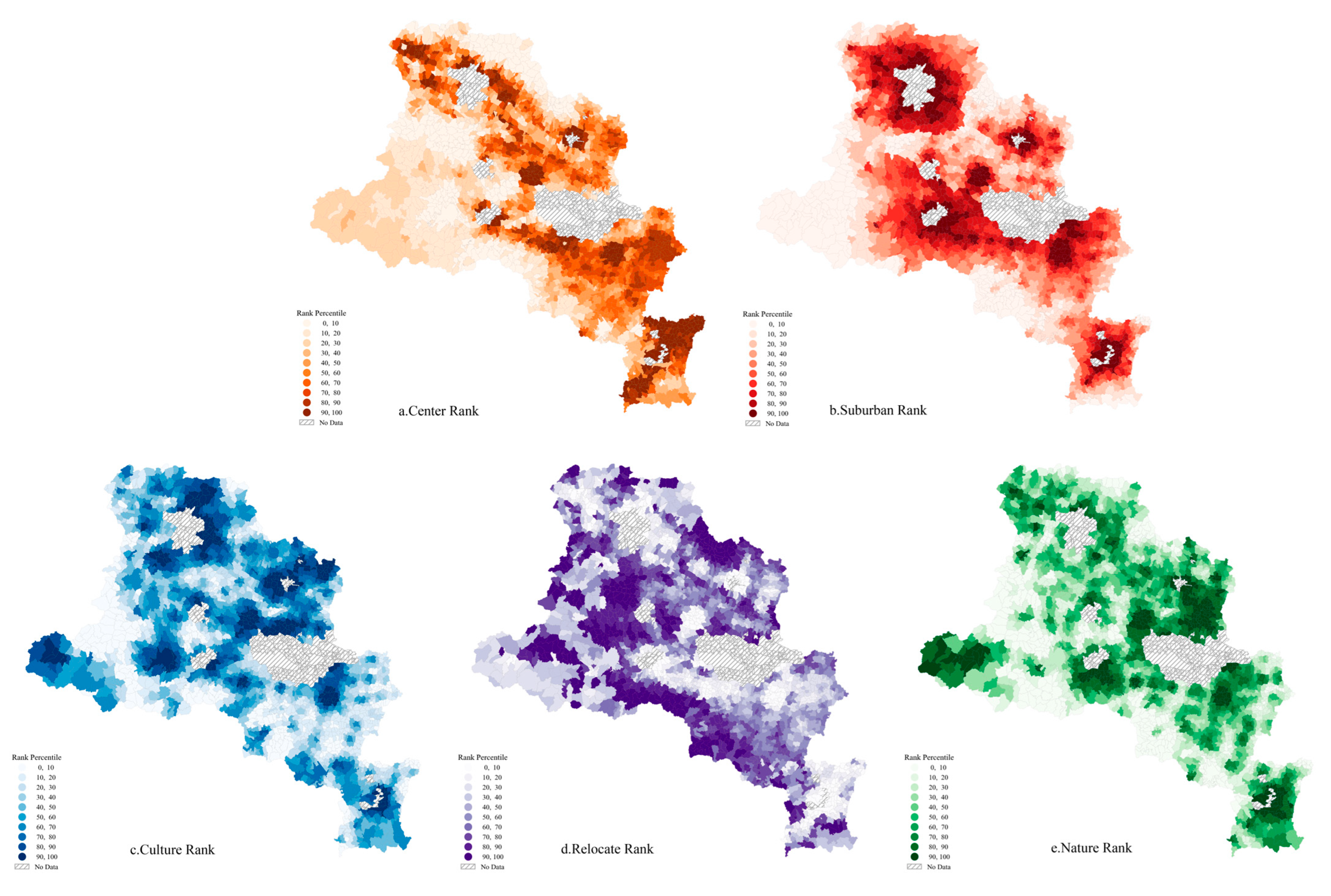
Based on the GPR values, villages are assigned to ten fixed decile intervals on the 0–100 percentile scale (i.e., 100–90, 90–80, …, 10–0), thereby generating a ten-level ordinal grading scheme for within-class comparison and spatial visualization. Since GPR is derived from the descending order of class-specific evidence values, this grading procedure reflects the relative positional hierarchy of villages within each functional category from a globally comparable rank perspective.

To facilitate cross-category comparison of evidential distribution patterns, the original class-specific evidence values are further min–max normalized to the interval [0, 1]. This normalization is introduced solely for cross-category comparability of curve morphology, rather than for redefining the ordinal rank structure itself. Accordingly, the horizontal segmentation of the analytical framework is determined by the GPR intervals, whereas the vertical profile of the evidential curves is represented by normalized evidence scores.

Under this design, the GPR-based grading maps and the normalized evidence curves jointly provide a unified basis for comparing the relative rank hierarchy and score morphology of different functional categories.

Finally, to examine the intersection, co-occurrence, and tradeoff relationships among the most salient functional carriers, spatial visualization and statistical correlation techniques (e.g., Pearson correlation utilizing continuous normalized evidence scores, and UpSet plots) are applied to salient-feature villages, operationally defined as the top 10% villages ranked by class-specific evidence within each category, which is rank-equivalent to the highest GPR interval (90–100). This threshold is intended to capture the most representative and strongly expressed manifestations of each rural function, thereby supporting a clearer diagnosis of cross-functional interaction structures among the core functional carriers.

3.4. Experimental Settings and Validation Protocol

This section specifies the experimental settings and validation protocol before the results analysis, including comparative models, implementation settings, parameter selection, and seed-sample construction. Three types of comparative models were introduced to evaluate the contribution of the proposed framework. PCA + K-Means was used as a non-topological baseline to assess the added value of graph-based spatial learning. GCN was used as a flat graph baseline to examine whether hierarchical village–township–city representation learning improves functional identification beyond local adjacency. HGI-Mean was constructed by replacing multi-head attentional aggregation with mean pooling, thereby testing the contribution of attention-based semantic aggregation. The complete model was denoted as HGI-MHA, and the selected four-head configuration was used as the main model in the results section.

All experiments were implemented using PyTorch v.2.6.0 Geometric on an NVIDIA RTX 4090 GPU. The model was optimized using Adam with an initial learning rate of 0.006 for 2000 epochs. A one-layer GCN encoder was adopted to reduce the risk of over-smoothing. Considering the spatial structure of the study area, urban nodes were retained during representation learning to capture urban spillover effects on surrounding villages, but were removed during village-level inference to avoid bias in functional classification. In the EDL module, a linear annealing strategy was applied to the KL-divergence regularization term, allowing the model to maintain fitting capacity in the early training stage while improving uncertainty calibration in later training.

To mitigate the influence of arbitrary parameter settings, key hyperparameters were determined based on related studies and targeted sensitivity checks. In the joint HGI objective, the balancing coefficient α was used to regulate the relative contribution of village–township and township–city mutual-information constraints. Candidate values of α = 0.1, 0.3, 0.5, 0.7, and 0.9 were tested, and α = 0.5 was selected because it provided a balanced weighting between local and global hierarchical constraints and produced stable model performance. In addition, HGI variants with k = 1, 2, 4, and 8 attention heads were compared to examine the influence of semantic subspace partitioning. The four-head configuration was selected according to the attention-head comparison reported in Appendix A Figure A1, and its final comparative performance is summarized in Section 4.2. It achieved balanced category-wise performance without introducing unnecessary model complexity. Detailed implementation settings and parameter-selection rationale are summarized in Appendix A 

Table A3. Implementation and hyperparameter settings with selection rationale.

Item	Setting/Checked Configuration	Selected Setting	Rationale
Deep learning framework	PyTorch Geometric	PyTorch Geometric version 2.6.0, with Python version 3.10, PyTorch version 2.4.0, and CUDA version 12.1	Used to implement graph neural network modules and hierarchical graph representation learning.
Hardware environment	GPU-based training environment	NVIDIA RTX 4090 GPU	Used to accelerate graph neural network training and repeated comparative experiments.
Optimizer	Adam	Adam	Supports stable optimization of neural network parameters under few-shot supervision.
Learning rate	Empirical training setting	0.006	Provided stable convergence during model training.
Training epochs	Empirical convergence setting	2000 epochs	Ensured sufficient convergence without unnecessary extension of training.
GCN encoder depth	Shallow graph encoder design	One-layer GCN	Reduces the risk of over-smoothing in graph representation learning.
Spatial input strategy	Urban nodes retained during representation learning and removed during inference	Urban nodes retained during representation learning and removed during inference	Captures urban spillover effects while avoiding bias in village-level classification.
HGI balancing coefficient α	α = 0.1, 0.3, 0.5, 0.7, 0.9	α = 0.5	Selected based on related studies and targeted parameter checks; provides a balanced weighting between village–township and township–city mutual-information constraints.
Attention-head configuration	k = 1, 2, 4, 8	k = 4	Selected according to the attention-head comparison reported in Appendix A Figure A1; achieved balanced category-wise performance without introducing unnecessary model complexity.
KL-divergence regularization	Linear annealing strategy	Linearly annealed from 0 to 1	Maintains early-stage fitting capacity and improves uncertainty calibration in later training.

.

To improve the reliability of few-shot supervision, the seed samples were constructed as planning-recognized and expert-verified semantic anchors rather than randomly selected labels. Candidate villages were first identified from statutory planning documents, official directories, and officially recognized village lists or project records. Specifically, Suburban seed samples were mainly selected from villages explicitly identified in statutory planning documents as being associated with urban-fringe development, urban-rural integration, or urban expansion zones. Center seed samples were selected from villages designated as central villages, key villages, or priority development villages in existing planning documents. Relocate seed samples were selected from villages where relocation, consolidation, or resettlement had already been implemented or planned. Nature and Culture seed samples were identified from villages with officially recognized or declared ecological, landscape, traditional, or cultural-resource attributes. After the initial screening, the candidate samples were further reviewed through consultation with planning experts, and only villages whose documentary evidence, spatial characteristics, and functional interpretation were consistent with the target category were retained. The detailed seed-sample validation protocol is provided in Appendix A 

Table A4. Seed sample selection and qualitative validation protocol.

Functional Category	Primary Evidence for Initial Selection	Qualitative Validation and Retention Criterion
Suburban	Villages explicitly identified in statutory planning documents as being associated with urban-fringe development, urban–rural integration, urban development axes/nodes, or urban expansion-related zones.	Candidate villages were retained only when the planning description and spatial context jointly indicated urban spillover effects, urban–rural integration, or suburban functional transition, rather than merely general development intensity.
Center	Villages designated as central villages, key villages, or priority development villages in existing statutory planning documents.	Candidate villages were retained only when the planning-recognized central role was consistent with their settlement agglomeration, public-service concentration, or regional coordination functions.
Nature	Villages officially recognized, declared, or planned as having ecological, landscape, natural tourism, or natural-resource attributes.	Candidate villages were retained only when the natural-resource attributes were explicit, dominant, and consistent with the Nature category, and when the documentary evidence and spatial-resource conditions supported this interpretation.
Culture	Villages officially recognized, declared, or listed as traditional villages, cultural villages, cultural heritage villages, or cultural-resource carriers.	Candidate villages were retained only when the cultural-resource attributes were explicit and traceable, and when sufficient documentary, spatial, or heritage evidence supported their assignment to the Culture category.
Relocate	Villages where relocation, consolidation, resettlement, or village layout adjustment had already been implemented or clearly planned in official documents or project records.	Candidate villages were retained only when the relocation-oriented planning intention was explicit and supported by actual implementation, project records, or clear planning evidence, rather than being inferred only from weak development conditions.

Note: Seed samples were used as high-confidence semantic anchors under the few-shot setting. Candidate villages were first identified from statutory planning documents, official directories, officially recognized village lists, or project records, and were then reviewed by planning experts. Only villages whose documentary evidence, spatial characteristics, and functional interpretation were consistent with the target category were retained.

.

4. Results

4.1. Spatial Patterns of Multidimensional Features

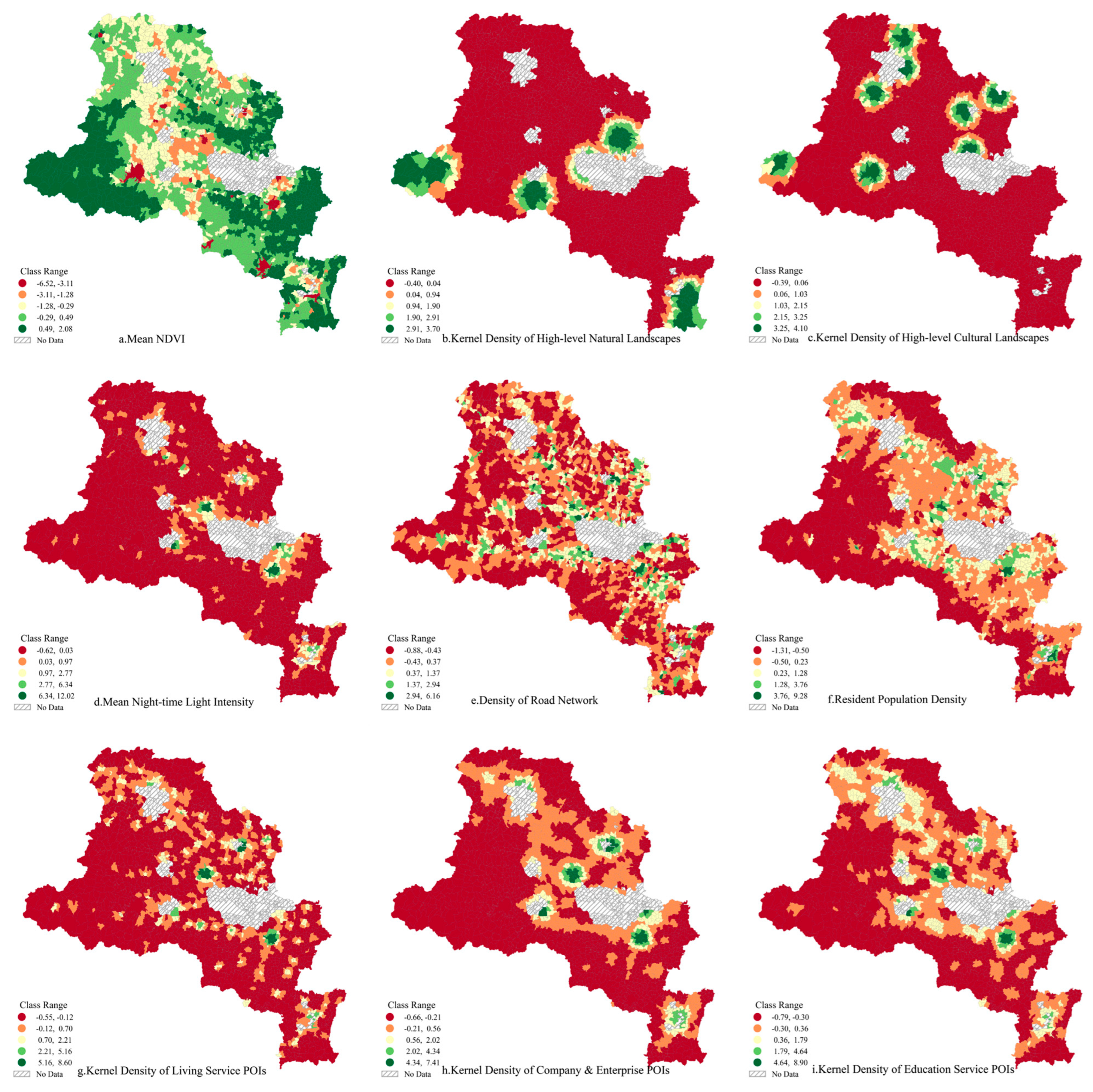
Based on the multidimensional feature matrix constructed in Section 3, nine representative indicators from three dimensions—natural background, socioeconomic vitality, and public service provision—were selected for spatial visualization. Figure 4 presents their spatial distributions in a 3 × 3 layout and provides the geographical context for interpreting the subsequent modeling results.

Natural and cultural resources showed a clear concentration in mountainous and hilly areas. As shown in Figure 4a–c, high NDVI values (Figure 4a) were concentrated mainly in the western and southern uplands, indicating relatively strong ecological conditions in these areas. A similar pattern was observed for the kernel density of high-level natural landscapes (Figure 4b), whose high-value clusters were distributed primarily along the western mountainous belt. High-level cultural landscapes (Figure 4c) were more spatially discrete, but several local clusters could still be identified in the central and northern hilly areas. Taken together, these patterns suggest that the western mountainous zone has relatively strong ecological and tourism-resource endowments, providing an important geographical basis for differentiated rural functions. Socioeconomic vitality and service facilities generally exhibited a center–periphery gradient. As shown in Figure 4d–i, high values of nighttime light intensity (Figure 4d), enterprise density (Figure 4h), and several service-facility densities (Figure 4g,i) tended to cluster around the central urban area and the eastern plain counties, indicating stronger economic activity and service concentration in these locations. However, population distribution and facility provision did not fully coincide across space. Although both showed local concentration near urban centers, resident population density (Figure 4f) formed a broader and more continuous distribution across the central and southeastern agricultural plains, whereas public service facilities remained more nodal and localized. This spatial mismatch suggests that, in some densely populated agricultural areas, facility provision may lag behind the scale of the resident population. Overall, the multidimensional features of the study area displayed marked spatial non-stationarity and substantial variation in the local combinations of natural, demographic, economic, and service-related elements. Western areas were characterized by stronger ecological conditions, the central and southeastern plains by broader population concentration, and eastern areas by higher levels of economic activity and service aggregation. At the same time, the differing spatial forms of population and facility distributions indicate that these feature combinations are also scale-sensitive. These patterns provide an important geographical backdrop for understanding the local dependencies captured by the subsequent hierarchical feature learning and spatial diagnostic results.

4.2. Overall Performance Comparison and Optimal Model Selection

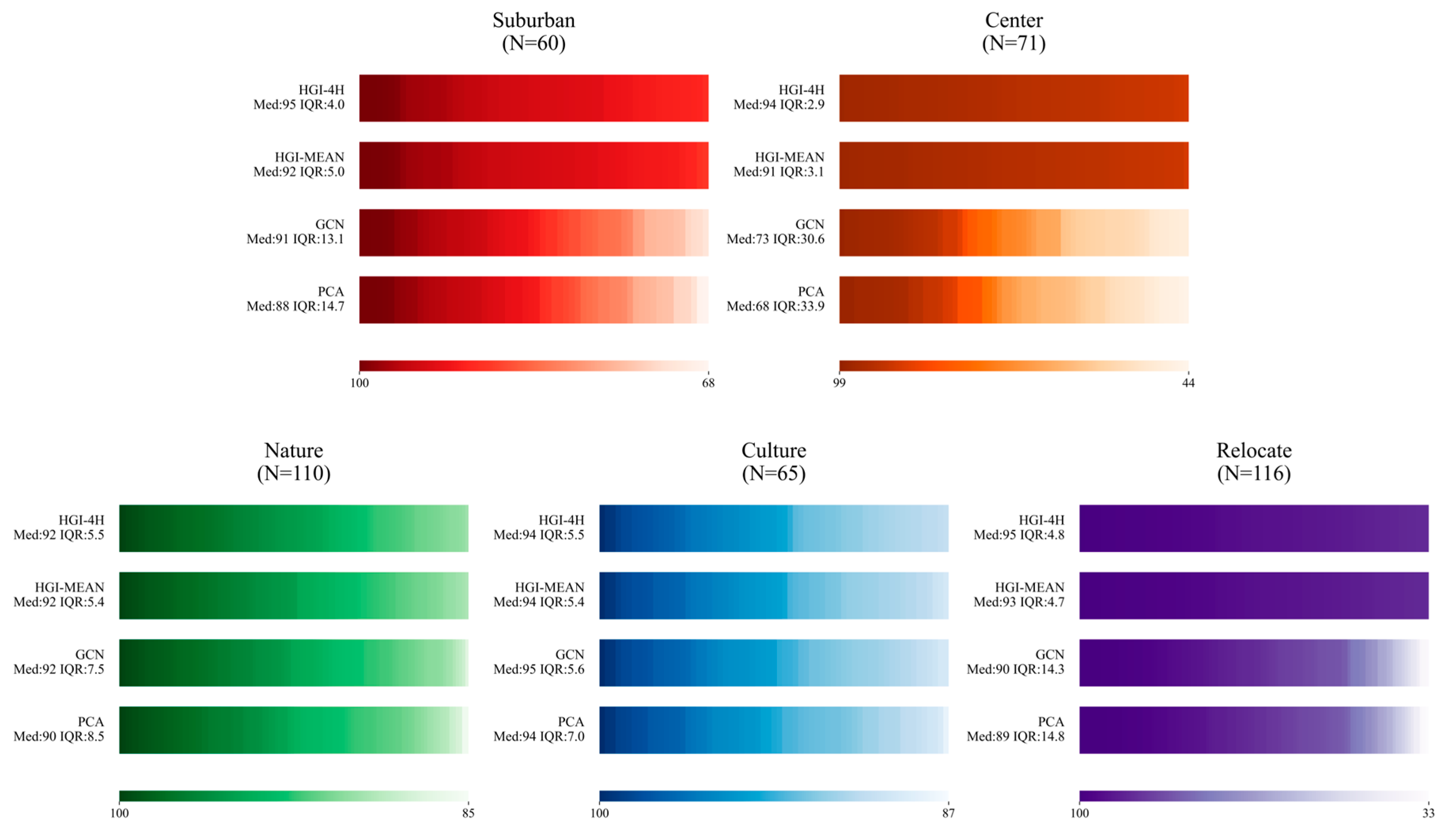
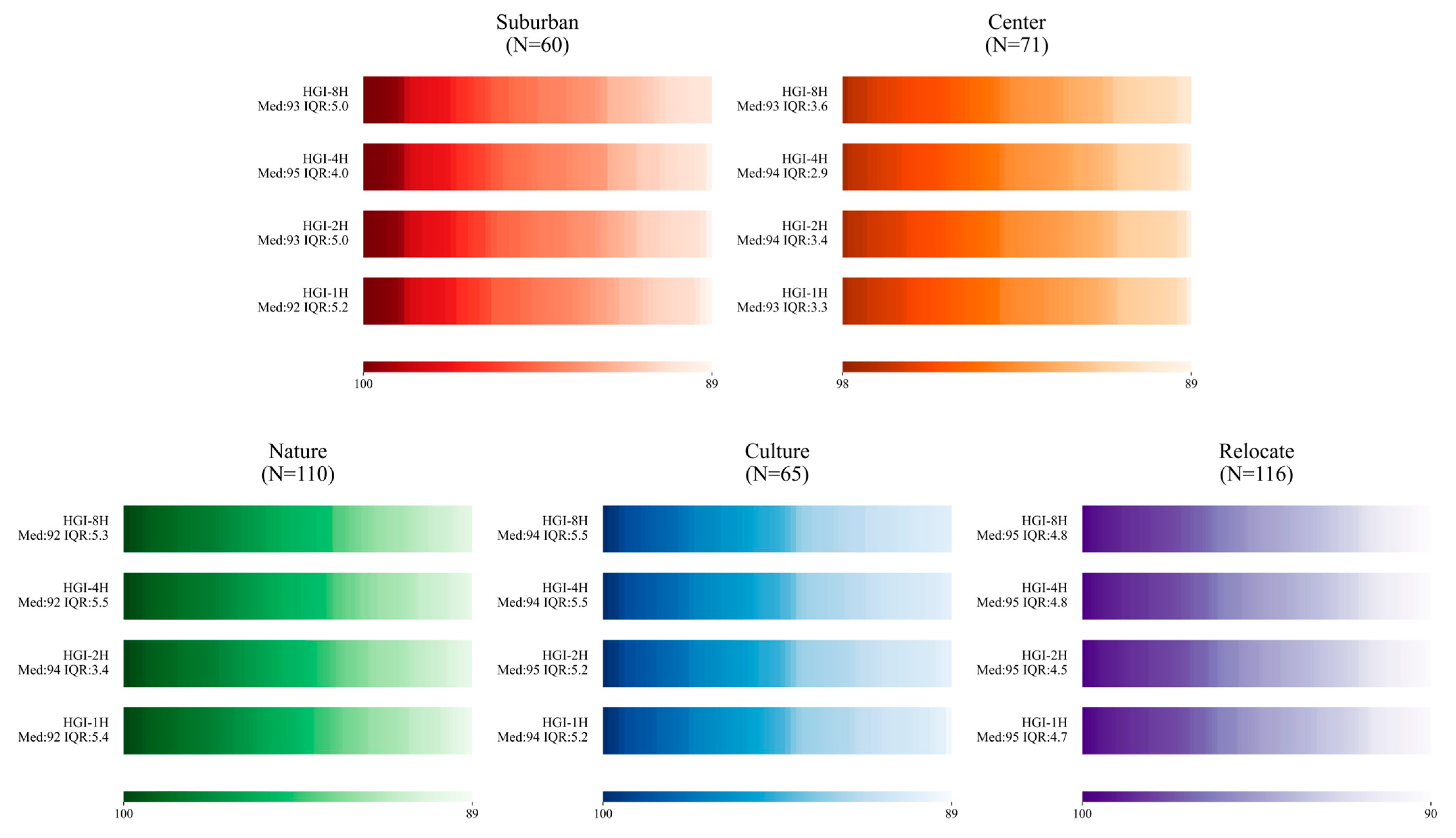
Figure 5 compares the category-wise rank distributions produced by different models under the few-shot setting. Overall, the HGI variants outperformed the baseline models (PCA and GCN) across all five rural-function categories. The most consistent advantage was the markedly smaller within-category dispersion, as reflected by lower interquartile ranges (IQRs). In contrast, the baseline models generally showed broader right-tail attenuation in several categories, indicating less stable behavior for lower-ranked or feature-ambiguous samples. By incorporating hierarchical spatial context, the HGI models produced more compact rank distributions, with IQR values generally below 5.5 across categories.

The magnitude of improvement varied across categories. The largest gains were observed in the Suburban, Center, and Relocate categories. For example, in the Center category, HGI-4H reduced the IQR from 30.6 in GCN to 2.9. In comparison, performance differences were narrower for the Nature and Culture categories, where even the baseline GCN already exhibited relatively compact rank distributions. In these categories, the HGI variants mainly provided further reductions in within-category dispersion rather than substantial shifts in the overall rank pattern.

Among the HGI variants, HGI-4H showed the most balanced overall performance. It achieved the lowest IQR in the Suburban and Center categories and remained competitive in the remaining categories. As shown in Appendix A Figure A1, although HGI-2H performed similarly to HGI-4H in some categories, HGI-4H showed the most consistent behavior across the full set of rural-function types considered in this study. On this basis, HGI-4H was selected as the optimal model configuration for the subsequent analyses.

4.3. Module Contribution Analysis Based on Rank Drift

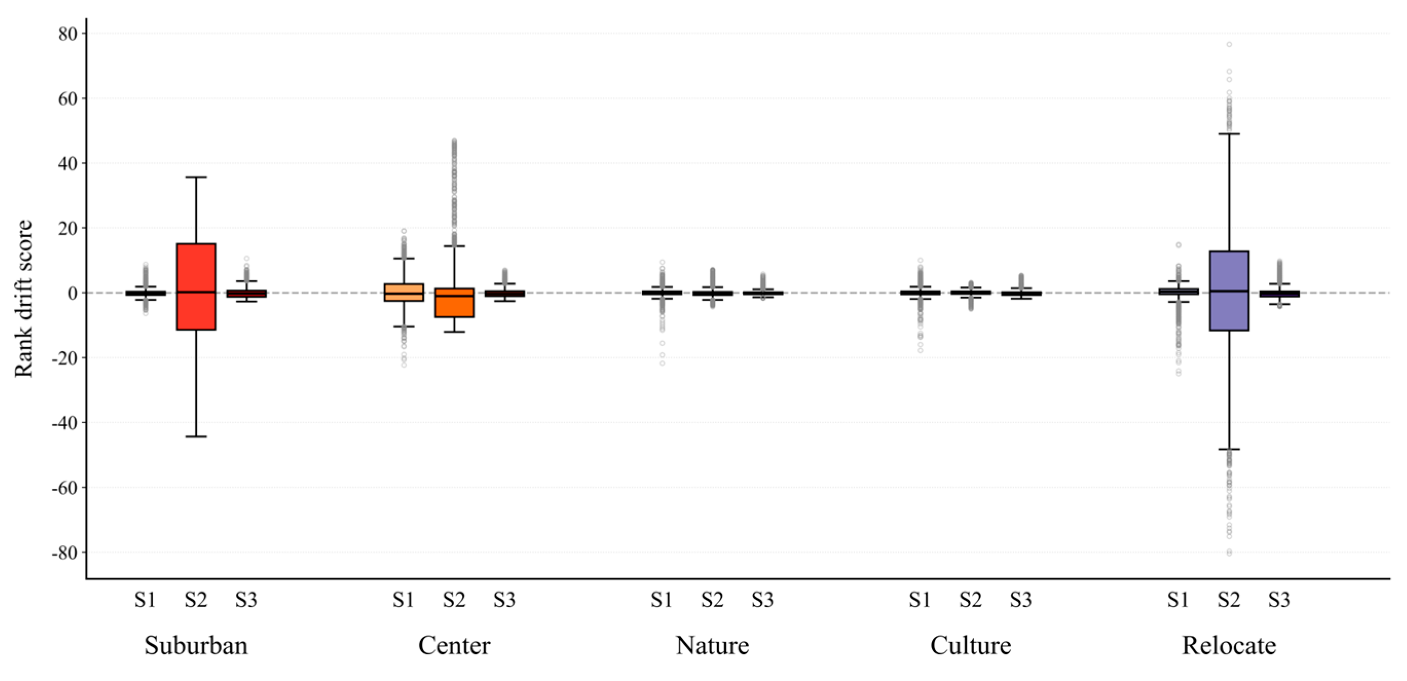
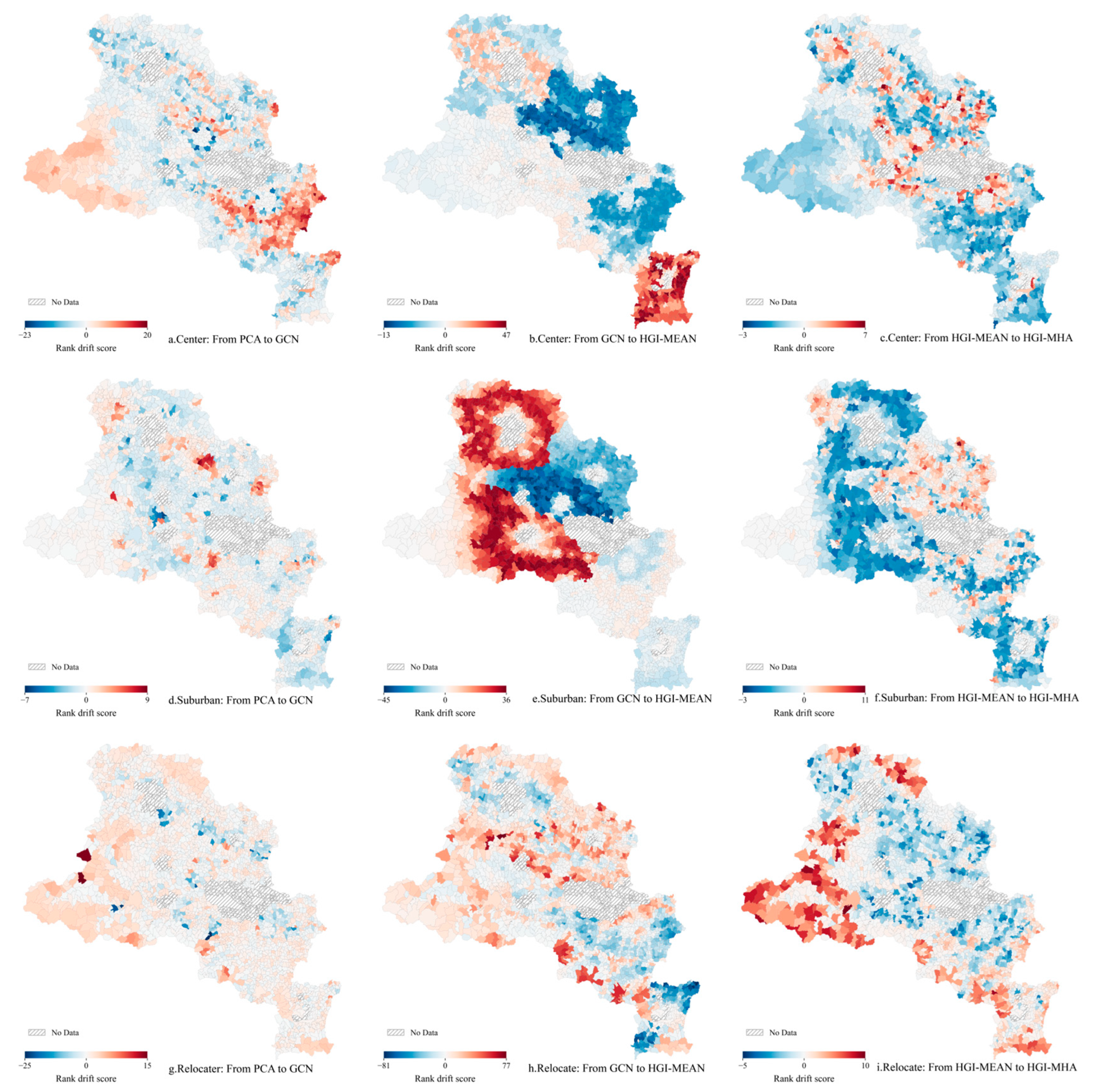
This section analyzes the effects of different model components on rural functional identification by tracking the rank drift ($\Delta Q_{i,k}$) during model evolution. To this end, the evolution process is divided into three progressive stages (corresponding to the boxplots in Figure 6 and spatial drift maps in Figure 7): S1 (Topology Introduction, PCA to GCN) is used to evaluate the initial contribution of geographical adjacency; S2 (Hierarchy Introduction, GCN to HGI-Mean) assesses the constraining effect of the township-city macro-context; and S3 (Semantic Enhancement, HGI-Mean to HGI-MHA) evaluates the fine-grained regulatory effect of the multi-head attention mechanism on micro-level features. Positive rank drift indicates that the corresponding model component increases a village’s relative functional rank, whereas negative rank drift indicates rank suppression. Values close to zero suggest minor adjustment or stable functional tendency, while larger absolute values indicate stronger correction effects and potential functional re-categorization.

The corrective effects of different model components showed marked non-uniformity, with S2 inducing the most pronounced shifts in rank distribution. As shown in Figure 6, the largest rank perturbations consistently occurred during S2. In particular, for the Suburban and Relocate categories, the interquartile ranges (IQR) of the drift scores widened substantially, indicating that the macro-context module effectively corrected a considerable number of samples that had been misjudged by the flat GCN. By contrast, the Nature and Culture categories maintained highly convergent drift distributions around zero across all stages. This pattern indicates that the identification of these two categories relies primarily on intrinsic local resource attributes rather than complex spatial structures, making them relatively insensitive to hierarchical and attention-based enhancements.

Suburban and Relocate villages constituted the main correction zones in S2. Combined with the spatial drift map (Figure 7e), the Suburban category exhibited a distinct pattern of spatially differentiated calibration during S2: villages along the western and northern urban fringes experienced significant rank increases (positive drift), whereas villages in the central plain hinterland underwent noticeable rank decreases (negative drift). This pattern suggests that conventional GCNs, which rely primarily on local neighborhood smoothing, tend to misclassify ordinary agglomerated villages in the central plains as suburban nodes. The introduction of the macro-context in S2 effectively suppressed these false-positive noise samples in the hinterland and amplified the true suburban signals along the urban spillover edges. Furthermore, the positive drifts produced by the multi-head attention mechanism in S3 (Figure 7f) demonstrate its ability to capture subtle feature variations that are obscured by mean pooling, thereby providing an additional fine-grained calibration. For Relocate, the S2 drift map (Figure 7h) shows that the hierarchical context further differentiated peripheral mountainous villages from ordinary low-accessibility villages, indicating that macro-contextual constraints helped clarify relocation-related functional signals.

The rank changes in Center villages spanned both S1 and S2, reflecting a two-stage identification process: “local agglomeration detection” followed by “macro-center confirmation.” The boxplots in Figure 6 showed that the Center category already displayed noticeable dispersion in S1, while the corresponding spatial maps (Figure 7a,b) revealed positive drifts in several western and southern areas. This finding indicates that introducing local topology (S1) helps preliminarily identify potential central places exhibiting neighborhood agglomeration effects. Upon entering S2, the ranks of this category diverged further, as reflected by multiple high-value positive outliers. This result confirms that the hierarchical structure (S2) is crucial for distinguishing true regional centers from ordinary local agglomerations, assigning higher identification confidence to nodes supported by macro-level centrality.

In summary, the performance improvements of the model stemmed from distinct component contributions: the hierarchical structure (S2) provided the primary gain by introducing macro-spatial constraints that resolved identification confusion in the more complex categories (Suburban, Relocate, and Center), whereas the multi-head attention mechanism (S3) delivered secondary gains by enhancing the expression of micro-specific features. By contrast, for resource-dependent categories (Nature and Culture), simple node attributes and local topology were largely sufficient.

4.4. Fine-Grained Feature Identification and Pattern Reconstruction

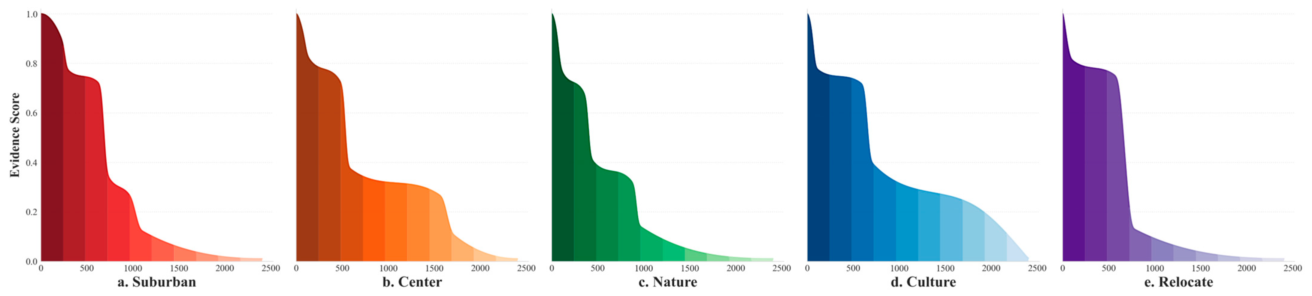
By jointly analyzing the evidence-normalized score curves (Figure 8) and GPR-based spatial grading maps (Figure 9), this section systematically delineates the statistical characteristics and spatial patterns of rural functional differentiation. The evidential score curves were utilized to characterize the distribution shapes and scarcity of the five functions in terms of numerical intensity, while the spatial grading maps illustrate their agglomeration patterns and heterogeneous structures in geographical space. The horizontal ordering follows the percentile-based GPR intervals, whereas the vertical axis represents min–max normalized evidence scores, enabling cross-category comparison of distribution morphology.

Combining the evidential score curves and spatial grading maps, the Suburban and Center villages exhibited distinct characteristics of annular dependence and multi-point support, respectively. Specifically, after an initial drop, the score curve of the Suburban category formed a relatively obvious intermediate platform in the 0.2–0.4 range. This statistical shape spatially corresponded to an annular distribution pattern tightly surrounding the central urban area and major townships, indicating the presence of numerous transitional semi-urbanized villages at the urban spillover zones. In contrast, the Center category was characterized by high-value areas coinciding with transport hubs and forming a widespread nodal distribution in the southern plains, with its score curve correspondingly showing a relatively gentle long-tail attenuation. These combined statistical and spatial features indicate that the formation of suburban and central functions is closely related to the urban-rural gradient and the distribution of transport nodes.

In the identification of Nature and Culture functions, high-grade areas were not entirely confined to the deep western mountains but exhibited a distinct near-city agglomeration feature. Spatially, a considerable number of high-grade villages were concentrated along the transport corridors surrounding the urban districts and county towns. The corresponding evidential curves further quantified this feature: the head of the Nature category was extremely high but narrowed rapidly, indicating the strong scarcity of core ecological resources; the Culture category presented a relatively obvious broad-shoulder shape, suggesting that high-grade cultural resources rely on broader spatial carriers than natural resources. This spatial distribution pattern indicates that the identification of high-grade ecological and cultural functions does not completely correspond to the static resource baseline, but is simultaneously influenced by both resource conditions and locational accessibility.

For the Relocate villages, the statistical curve exhibited a distinct cliff-like drop pattern. The curve rapidly dropped to near zero after approximately the 30% position of the global distribution, with almost no obvious transition zone. This binary statistical feature spatially corresponded to clear high-value areas in marginal mountainous regions, meaning that high-grade samples were primarily confined to mountainous fringes with large topographic reliefs and relatively weak infrastructure, forming a distinct spatial separation from the other four functions. This result indicates that the formation mechanism of the Relocate function is more strongly influenced by the combined effects of topographic constraints and insufficient development conditions.

4.5. Multi-Feature Correlation and Functional Composition Patterns

This section analyzes the compound characteristics and composition patterns of rural functions from three dimensions: attribute interaction, quantitative structure, and spatial pattern. Through a joint interpretation of correlation analysis, UpSet plots, and spatial distribution maps, it further identifies the co-occurrence relationships, quantitative structures, and geographical differentiation among different functions.

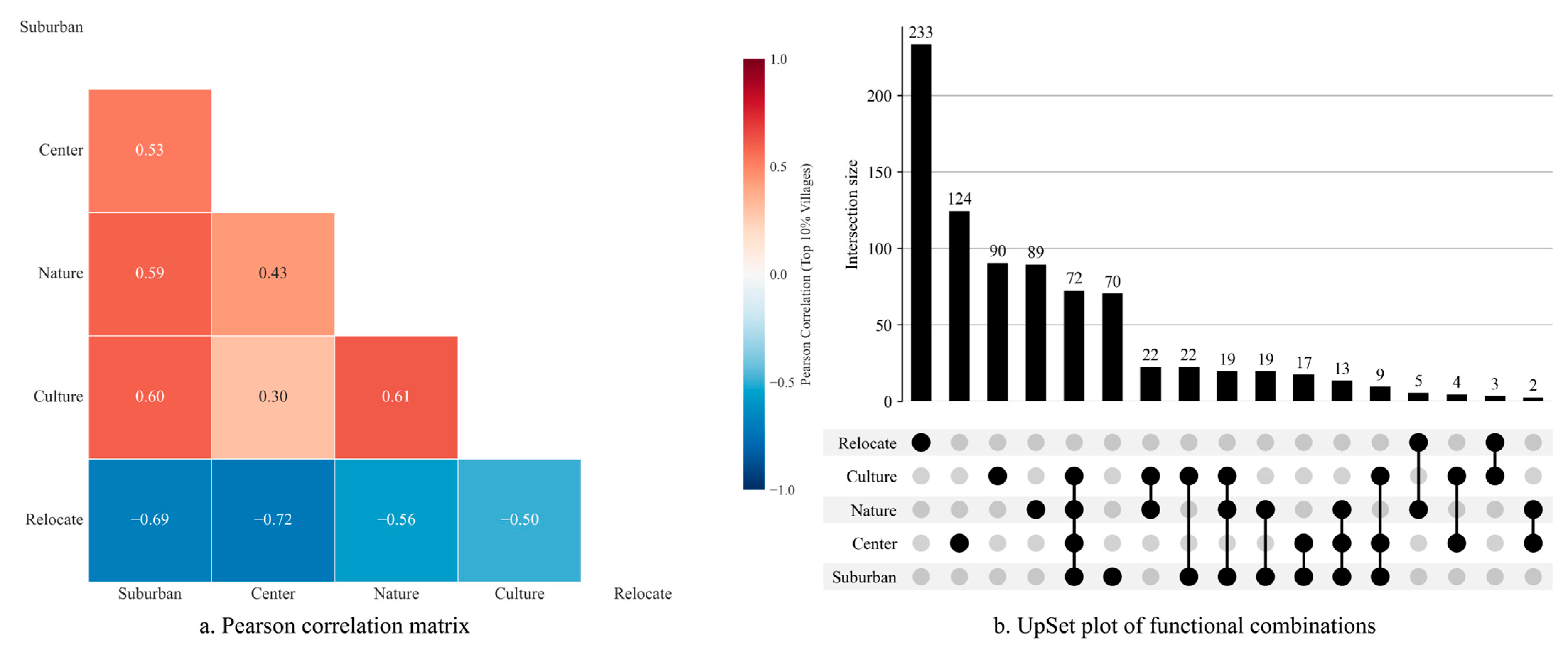
Based on the Pearson correlation analysis of salient-feature villages (utilizing their continuous normalized evidence scores) (Figure 10a), distinct synergy–trade-off relationships emerged among different rural functions. Here, salient-feature villages refer to the top 10% villages ranked by class-specific evidence within each category, corresponding in rank terms to the highest GPR interval (90–100). As shown in Figure 10a, the Suburban, Center, Nature, and Culture categories all exhibited significant positive correlations (r > 0.3), reflecting a strong co-occurrence tendency among these functions. Notably, the correlation coefficients between Suburban and Nature/Culture (r ≈ 0.6) were markedly higher than those between Center and these two categories, indicating a stronger coupling relationship between suburban functions and ecological/cultural functions. In contrast, the Relocate category exhibited significant negative correlations (r < −0.5) with the other four categories, demonstrating a clear statistical trade-off between the relocation function and other endogenous development functions.

The UpSet plot (Figure 10b) further quantifies the quantitative structure of functional combinations, revealing that single-function dominance remains the primary modality of the current rural territorial system. The results showed that “single Relocate” and “single Center” dominated in quantity, indicating that single-function dominance remains prevalent within the salient-feature subset. Conversely, within the compound functional combinations, the frequencies involving Suburban were significantly higher (e.g., “Sub+Nat” and “Sub+Cen” were highly common). This result indicates that the suburban attribute is a crucial concomitant variable in the compounding process of rural functions; compared to traditional agricultural villages, villages with suburban attributes are more prone to superimposing ecological or leisure service functions.

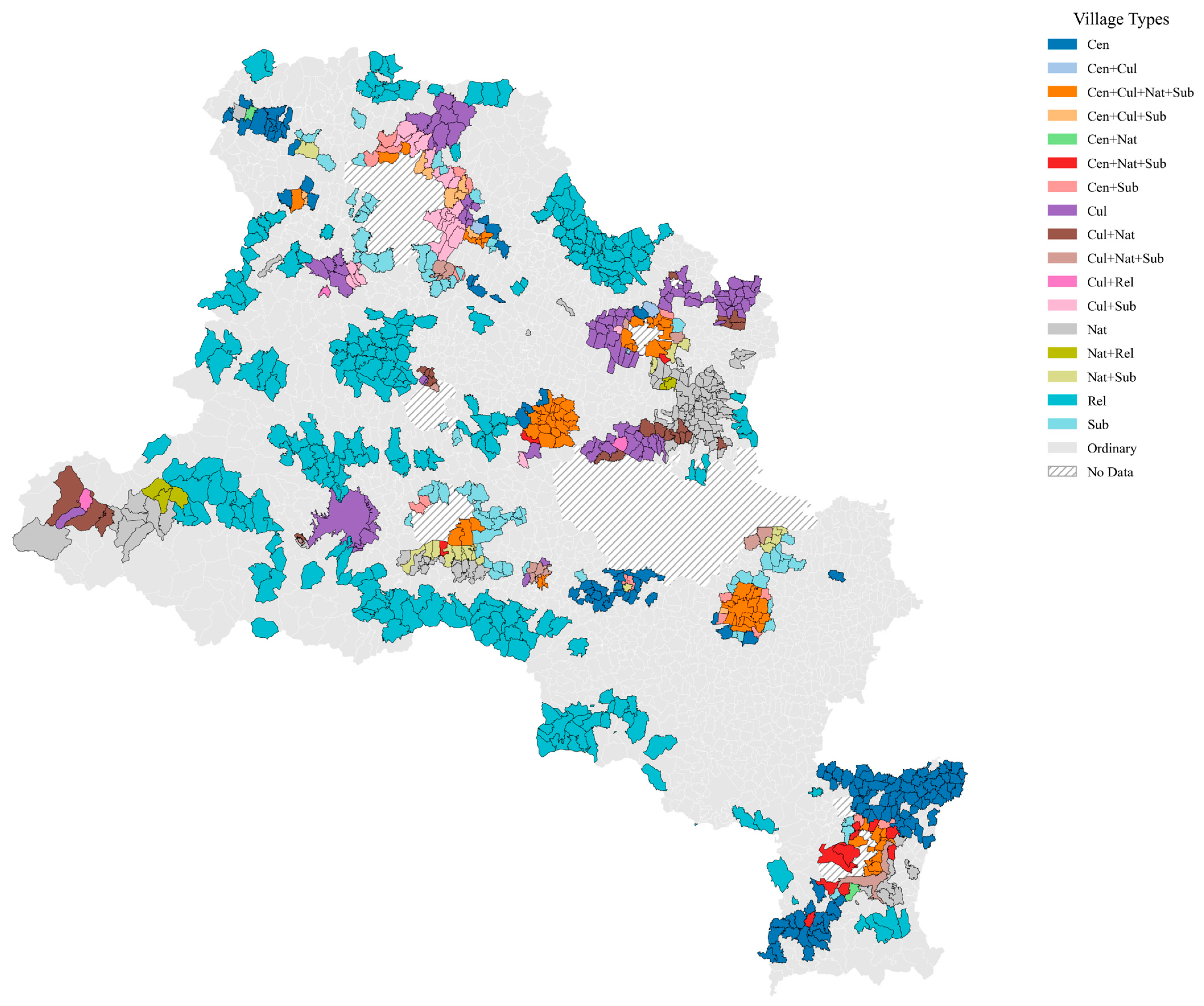
Geographically, functional combinations exhibited distinct characteristics of regional differentiation and annular mosaic (Figure 11). As illustrated in Figure 11, the Relocate function displayed a prominent edge-agglomeration feature, being widely distributed in peripheral areas with complex terrain and forming relatively clear spatial isolation patches. A more significant spatial variation occurred within the Center function: the southern plain agricultural area was dominated by the “single Center” type, primarily undertaking basic production and service functions; whereas near the urban development axes in the central–northern region, the central function more frequently superimposed suburban, cultural, and ecological attributes, forming multidimensional compound forms such as “Cen+Cul+Sub”. This spatial differentiation indicates that the closer a village is to the urban development axis, the more prone the central function is to superimposing other characteristic attributes, thereby exhibiting a higher degree of functional compounding.

5. Discussion

5.1. Methodological Value for Identifying Functional Differentiation in Rural Territorial Systems

The main value of FH-GRL is that it identifies village functions within a multilevel rural system rather than from village attributes alone. In rural territorial systems, village functions are shaped by both local conditions and wider spatial context. FH-GRL addresses this point by combining hierarchical graph learning with evidential inference. As a result, it tackles two common weaknesses in earlier village classification studies: the weak representation of spatial relations and the limited ability to show within-class differences [18,20,59,60,80].

The advantage of the framework is most visible when it is compared with flat clustering and flat graph models. The issue is not only whether FH-GRL produces better classification results in the present case. More importantly, it changes how village functions are interpreted. The HGI module places each village in a village–township–city structure, so local features are read together with higher-level context. The rank-drift results in Section 4.3 show this clearly. After hierarchy is introduced, many villages in the central plain hinterland no longer receive inflated suburban signals, while villages along the actual urban spillover edge are identified more clearly. This pattern matters because a flat model may confuse local agglomeration with true suburban influence. FH-GRL reduces that confusion by adding macro-context to local neighborhood information. This is especially useful for villages whose functional profiles are transitional or ambiguous [41,61,81,82]. Nevertheless, these results should be interpreted as evidence of methodological improvement within the present case study, rather than as proof of universal superiority across all rural regions.

A second value of the framework lies in its ability to move from hard classification to continuous grading. Many traditional methods end with discrete labels, so they show category membership but not the strength of a function within the same class [80,83,84]. FH-GRL adds GPR-based ranking on top of evidential learning, which makes within-class variation visible. The score curves in Section 4.4 illustrate this point well. The Suburban category contains an intermediate platform rather than a sharp break, and the Culture category shows a broader shoulder. These shapes suggest that many villages are neither clear core cases nor simple background cases. They lie in intermediate positions. For planning practice, this distinction is important. It helps separate core intervention areas from transitional areas and long-term reserve areas, instead of treating all villages in one class as equivalent.

The few-shot design also has clear limits, and these limits should be stated directly. FH-GRL reduces the need for large labeled datasets, but it still depends on the quality and representativeness of the initial seed villages. The semantic direction of the model can change with the seed set. For example, Relocate seeds selected mainly from disaster-prone areas may push the model toward ecological fragility, while seeds selected from shrinking settlements may strengthen signals of social decline. This sensitivity should not be seen only as a technical weakness. In planning-oriented classification, high-confidence labels are costly, expert-dependent, and often tied to local policy priorities. This means that FH-GRL is better understood as a transferable analytical logic than as a fixed template that can be copied unchanged across regions.

At present, the interpretation of FH-GRL still relies mainly on output-level diagnostics, including rank drift, GPR distributions, and spatial pattern comparison, rather than on a full explanation of the internal embedding space or attention weights. This limits the transparency of the learned representations for direct planning use. In practical applications, the framework may therefore be more feasible as a decision-support workflow: technical teams can handle model training and parameter updating, while planning agencies use the resulting functional maps, GPR rankings, uncertainty information, and diagnostic outputs for screening, comparison, and field review. Future work should further combine active learning, attention-weight interpretation, feature attribution, and cross-regional adaptation, so that the framework can rely less on expert-selected seeds and provide more transparent and robust support for heterogeneous rural settings [85,86,87,88].

5.2. Geographical Logic of Village Functional Differentiation: Synergy, Dependence, and Endogenous–Exogenous Dynamics

The results in Section 4.4 and Section 4.5 suggest that village functions are not shaped by a single dominant factor. Instead, they emerge through the combined effects of resource endowments, locational conditions, accessibility, development foundations, and planning interventions [89,90,91]. In this sense, village functional differentiation is better understood as a coupled spatial process than as the outcome of one isolated village attribute. Based on the empirical results, the geographical logic of this differentiation can be discussed from three related aspects: cumulative advantage, functional dependence, and endogenous–exogenous dynamics.

First, the results point to a clear pattern of cumulative advantage [91,92,93]. The correlation analysis shows that the Suburban, Center, Nature, and Culture categories are positively related, and the spatial maps also reveal visible compound belts across these functions. This pattern suggests that villages with better locational conditions are more able to convert ecological, cultural, or industrial-resource advantages into actual functional strengths. Resource endowments alone are often not sufficient. In most cases, they need traffic accessibility, market connection, and infrastructure support before they can develop into strong village functions [46,94,95,96]. This also helps explain why many compound villages are concentrated around towns and accessible corridors rather than in remote hinterlands. Here, location works not simply as a background condition, but as an amplifier of resource accumulation and functional clustering. In Pingdingshan, this mechanism is further shaped by the city’s resource-based industrial background. Mining and industrial development have historically influenced transport corridors, enterprise agglomeration, employment opportunities, and service provision in surrounding rural areas. These conditions may strengthen the industrial and service foundations of some villages, thereby contributing to Center, Suburban, or compound functional attributes. At the same time, mining-related constraints such as land subsidence, soil degradation, contamination risks, and ecological restoration pressure may also restrict rural development capacity. These negative effects were not fully captured in the current indicator system because consistent village-scale data on soil quality, contamination, and subsidence were not available, which should be regarded as an important limitation for resource-based regions.

Second, the results show a pattern of functional dependence, especially in the relation between suburban and cultural functions [61,97,98]. The annular pattern of the Suburban category in Section 4.4 indicates that suburban villages are not defined only by physical urban expansion. They also mark places where urban and rural factors interact in both directions. At the same time, the UpSet results in Section 4.5 show that high-value cultural villages rarely appear alone. They more often overlap with Suburban or Center attributes, especially in combinations such as Sub+Cul. Together with the broad-shoulder shape of the Culture curve in Section 4.4, this pattern indicates that cultural resources become strong village functions not only because of their intrinsic value, but also because of the accessibility, interaction opportunities, and nearby demand that allow those resources to be functionally realized. By contrast, a cultural site in a remote area may still have high intrinsic value, yet it is less likely to become a dominant development function when urban–rural linkages, tourism demand, and service accessibility remain weak [99,100,101]. Therefore, functional dependence does not mean that one function mechanically determines another. Rather, it suggests that certain functions are activated more effectively when local resources are connected to broader accessibility and service networks.

Third, the results suggest a dual endogenous–exogenous logic in the formation of Center villages [102,103,104,105,106]. Section 4.5 shows a clear contrast between the southern plains and the central–northern part of the study area. This contrast can be understood by linking Central Place Theory with the contemporary space-of-flows perspective. In the traditional central-place logic, rural centers mainly serve surrounding hinterlands through agricultural production support, daily services, and basic public facilities. In the southern plains, many Center villages appear as single-function villages. This pattern fits the stronger cultivated land base and population support of that region, suggesting that these villages mainly serve the surrounding agricultural hinterland. They can therefore be understood as endogenous production or service centers. By contrast, Center villages near the central–northern urban development axes more often overlap with Suburban and other attributes. In these places, the center function depends not only on local service provision but also on urban consumption spillovers, industrial linkages, logistics accessibility, and external commercial demand. These villages are therefore closer to exogenous service centers, whose functions are strengthened by their connection to wider urban–rural interaction channels rather than by local hinterland demand alone [103,104,105,107].

This interpretation is also related to the modeling logic of FH-GRL. The framework does not directly measure actual factor flows, such as commuting, logistics, tourist movements, or socio-economic interactions. However, the graph topology, village–township–city hierarchy, and indicators such as road-network density, Euclidean distances, POI-based KDE, and nighttime light intensity allow the model to capture flow-related spatial dependencies and potential interaction conditions. Therefore, the discussion of the “space of flows” should be understood as an interpretation of potential flow-related spatial relations rather than a direct measurement of dynamic flows. Future research should incorporate dynamic data, such as commuting records, mobile phone signaling, logistics flows, tourism trajectories, or platform-based transaction data, to verify how actual movement and interaction processes reshape village functions over time.

Overall, the results indicate that village functional differentiation follows a mixed geographical logic. Some functions depend more strongly on local resource conditions, whereas others are strengthened, or even activated, by external accessibility, industrial linkages, and urban–rural interaction opportunities. For this reason, rural functional analysis should pay attention not only to the space of places, but also to the potential interaction conditions associated with the space of flows. It should also distinguish villages that rely mainly on internal resource bases from those whose functions are more strongly activated by urban linkages, industrial networks, or external service demand.

5.3. Implications for Differentiated Governance and Rural Planning

The identified patterns of village functional differentiation provide a practical basis for differentiated governance and rural planning. The results indicate that rural functional variation is shaped by the combined effects of resource endowments, locational conditions, and development foundations. These differences are not random. They reflect visible gradients, functional combinations, and distinct village roles within the rural territorial system. For this reason, a uniform planning approach is unlikely to match the actual needs of different villages [32,41,104,108]. Based on the quantitative results of this study, the planning implications can be discussed from three aspects: tiered allocation, category-specific guidance, and linked multifunctional development.

First, the continuous functional intensity spectrum derived from EDL can be used to support a gradient-based intervention system. When the evidential score curves are read together with the ranking results, villages can be grouped into three broad intervals: High-Intensity Core Zones (top 10%), Potential Transitional Zones (10–50%), and General Reserved Zones (bottom 50%). These specific thresholds are not rigid mathematical constants, but rather heuristic cutoffs derived from the natural breaks in the evidential score curves (Section 4.4) and aligned with general local planning practices, where typically only a small fraction of rural settlements are selected as priority demonstration projects. In practical planning applications, these boundaries can be dynamically adjusted according to county-level land quotas and municipal investment capacities. Furthermore, the uncertainty scores generated by the EDL module can be used to refine these boundaries. For example, a village positioned near the 11% cutoff mark with high classification uncertainty should not be mechanically downgraded to a lower tier; instead, it flags a need for manual field verification by planning experts to determine its true developmental potential. High-Intensity Core Zones represent the strongest carriers of each function and may therefore be prioritized in demonstration-oriented rural revitalization programs, with stronger support in project allocation, land quotas, and industrial investment. Potential Transitional Zones correspond more closely to the intermediate parts of the score curves, where villages show some functional basis but still face clear weaknesses. In these cases, the priority is not large-scale expansion but targeted improvement. For example, villages with a relatively strong ecological base but weak suburban linkage may benefit more from better transport and service access, which can improve accessibility and help convert raw resources into actual functions. By contrast, villages in the General Reserved Zones are better suited to a strategic reserve approach that focuses on basic public services and improvements to the living environment rather than high-intensity construction input [107,109,110,111].

Second, governance measures should be adjusted to different village types and regional contexts. For Suburban villages, their annular distribution and dependence on urban proximity suggest that they should be guided more carefully as urban leisure hinterlands or industrial support areas, so that semi-urbanization does not proceed in a disorderly way [41,112,113]. For Center villages, the strategy should reflect the spatial contrast identified in Section 4.5. In the southern plain agricultural area, many Center villages function mainly as endogenous production centers, so governance may give priority to agricultural machinery services, storage, logistics, and other facilities that strengthen support for scaled agricultural production. In the central–northern urban axes, however, Center villages are closer to exogenous service centers. In these areas, greater emphasis may be placed on education, healthcare, and related public services in order to improve service capacity and population attraction. For Relocate villages, their strong spatial separation from other functional types and the steep decline in their rank curves suggest that a smart-shrinkage pathway is more appropriate. In practice, this may include guiding population concentration toward better-conditioned central villages and promoting spatial resource reallocation through demolition, consolidation, and land remediation [104,110,114,115]. However, given the significant social and administrative implications of rural relocation, this pathway must be applied with extreme caution by utilizing the model’s uncertainty-aware nature. For villages with high “Relocate” scores but also high uncertainty, planning authorities should avoid aggressive, top-down spatial intervention. Instead, these areas should be temporarily classified under a “conditional maintenance” status, requiring further public consultation, detailed socio-economic surveys, and ground-truth investigations before any irreversible consolidation is implemented.

Finally, villages with multifunctional combinations require linked development pathways rather than single-function planning. The results in Section 4.5 show that some functions, especially those with suburban attributes, often overlap with cultural, ecological, or central functions. This means that village development should not be planned only around one dominant label. It should also consider how multiple functions reinforce one another under favorable locational conditions. For compound villages with suburban attributes, a pathway that combines characteristic resources with commercial services may be more suitable, because these villages already have relatively better infrastructure and market access for turning ecological and cultural resources into economic value. At the same time, public service improvement can be combined with center strengthening in order to increase the radiating capacity of compound nodal villages. In plain agricultural areas, a linked pathway based on agricultural management and scale consolidation may also be appropriate, using the agglomeration effect of central villages to support contiguous land governance, technology diffusion, and organizational coordination. Through such linked arrangements, multifunctional synergy can become a practical way to improve the efficiency and adaptability of rural territorial systems.

6. Conclusions

This study addresses village functional differentiation under two common conditions in rural planning research: strong spatial heterogeneity and limited labeled samples. To do so, it develops and tests an FH-GRL framework that combines hierarchical graph learning with evidential inference. The framework moves village identification from flat modeling to multilevel representation and from discrete classification to continuous functional grading. Based on the empirical results from Pingdingshan City, three main conclusions can be drawn.

(1) Cross-scale context improves the identification of village functional differentiation within the present case study.

The FH-GRL framework captures the relational structure embedded in the village–township–city hierarchy. The results indicate that hierarchical context works as a spatial calibration mechanism. It reduces pseudo-suburban signals in the central plain hinterland and improves the identification of villages that are more directly shaped by urban spillovers. This result suggests that village functions can be identified more effectively when local attributes are interpreted within a broader multilevel structure rather than in isolation.

(2) Rural functional differentiation reflects both place-based conditions and potential flow-related linkages.

The results show a clear differentiated pattern among Center villages. In the southern agricultural plains, Center villages mainly function as endogenous production or service centers supported by cultivated land, population bases, and local hinterland demand. Along the central–northern urban axes, they are more likely to function as exogenous service centers influenced by urban consumption spillovers, industrial linkages, and external service demand. More generally, village functions are shaped not only by local resource conditions, but also by locational position and potential urban–rural interaction conditions. However, these flow-related interpretations are based on static spatial proxies and graph-based relational structures rather than direct measurements of dynamic factor flows.

(3) Continuous grading provides diagnostic support for differentiated governance and resource allocation.

The GPR-based evaluation system makes it possible to distinguish not only village categories, but also differences in functional intensity within the same category. This helps identify high-intensity functional carriers, potential transitional villages, and general reserve areas under different functions. In planning practice, such graded outputs can support more targeted diagnosis and priority screening instead of uniform intervention. However, these results should be used as planning-support evidence rather than as direct planning decisions or statutory thresholds, especially for villages near classification boundaries or with high model uncertainty.

The framework also has several boundary conditions. First, although FH-GRL performs well in the Pingdingshan case, its superiority is mainly supported by internal diagnostic metrics and case-based spatial interpretation; external validation across different regions remains limited. Second, the semantic alignment of the model still depends on the quality and representativeness of few-shot seed samples, which means that expert knowledge and local planning context remain important. Third, the results are sensitive to data availability and spatial scale. Due to the lack of consistent village-scale data, this study did not fully incorporate soil quality, contamination, mining subsidence, land suitability, or actual dynamic flows such as commuting, logistics, tourism movements, and socio-economic interactions. These limitations may affect the interpretation of rural functions in resource-based regions and constrain the transferability of the framework. Future research should therefore focus on active learning, cross-regional validation, scale-sensitive modeling, dynamic flow-data integration, and region-specific indicator expansion. These directions would help improve the transparency, robustness, and practical value of FH-GRL for dynamic rural planning.