Ecosystem Services–Human Well-Being Coupling in China’s Northeast Black Soil Region: A Two-Level Perspective Incorporating Internal Ecosystem Service Balance

Abstract

There exists a complex and intimate interplay between ecosystem services and human well-being. This coordination not only concerns regional sustainable development but also depends on the structural balance of various service functions within ecosystems. Therefore, based on three-phase data from 2000 to 2020, this study investigates the coupling coordination relationship between ecosystem services and human well-being in the Northeast Black Soil Region, along with its driving factors and influence pathways. Key ecosystem services and human well-being levels were quantified, introducing a two-level coupling coordination model: D1 (coordination between total ecosystem service provision and human well-being) and D2 (coordination between internal ecosystem service balance and human well-being). Results indicate that: (1) From 2000 to 2020, the Ecosystem Service Index showed an initial rise followed by a decline. Synergistic relationships among ecosystem services strengthened, while trade-offs between cultural services (Shannon diversity index) and other services persisted. High human well-being zones were highly concentrated in provincial capitals, indicating the gradual formation of a priority development pattern. (2) The coupling coordination level of D2 was significantly weaker overall than that of D1. Compared to the overall supply level, the coordination of internal ecosystem service functions was a more critical factor constraining regional comprehensive development. (3) Landscape patterns are the primary factor governing the coupling relationship between regional ecosystem services and human well-being. Future efforts should focus on optimizing landscape configurations to enhance both human well-being and ecosystem coordination. This study contributes to a better understanding of the relationship between ecosystem services and human well-being from the perspectives of both aggregate coordination and internal balance, and also provides valuable insights for research and management measures in regions characterized by intensive agricultural development and rapid urbanization.

1. Introduction

Globally, human activities are altering Earth’s ecosystems at an unprecedented scale and pace, triggering a series of ecological and environmental issues including biodiversity loss, land degradation, water scarcity, and climate change [1]. These changes not only undermine ecosystem stability but also diminish their capacity to deliver critical ecosystem services (ESs) to humanity, posing severe challenges to the sustainable advancement of human well-being (HWB). Against this backdrop, elucidating the interactive mechanisms between ESs and HWB has emerged as a central research topic in sustainable development studies.

Ecosystem services refer to the various benefits provided to humans by natural ecosystems through their functions [2], typically categorized into four major types: provision, regulation, support, and cultural services [3]. Human well-being, meanwhile, comprehensively reflects the overall state of humanity across material, spiritual, social, and environmental dimensions [4]. Extensive research indicates [5,6] that ESs form the material foundation and ecological safeguard underpinning HWB, while their dynamics significantly influence human quality of life. These two elements interact through complex feedback mechanisms, constituting a prototypical human–land coupling system [7]: on one hand, the provisioning capacity of ESs constrains improvements in HWB; meanwhile, human actions such as land-use changes and policy interventions shape ecosystem structure and service functions [8]. This bidirectional interaction can generate synergistic effects but may also trigger trade-offs in services and ecological risks, directly impacting regional sustainable development capacity. For instance, afforestation programs enhance carbon storage and soil conservation, thereby safeguarding food security, yet may also induce trade-off conflicts [9]; agricultural expansion boosts food yields in the short term but sacrifices habitat quality and biodiversity [10]. Therefore, understanding the operational mechanisms and evolutionary patterns of this coupled system is the scientific prerequisite for reconciling the contradictions between ecological conservation and socioeconomic development.

In recent years, quantitative assessments of the relationship between ecosystem services and human well-being have been extensively conducted across various spatial scales. However, existing research still faces several limitations. First, most studies focus on changes in the total supply of ecosystem services or on individual services to examine their relationship with human well-being, thereby overlooking the coordination among different functions within the ecosystem service system. An increase in the total supply of ecosystem services in a region does not necessarily imply an overall improvement in the ecosystem. For instance, Yang et al. (2025) [11] analyzed the interactive relationship between ESs and HWB in China’s Yellow River Basin; Li et al. (2024) [12] found that the sustained decline in regulating services was masked by the expansion of provisioning services, leading to structural imbalances within the system. An overall increase in ES levels may be driven by the excessive expansion of a single service category, making it difficult to reflect the balanced state of ecosystems and their comprehensive impact on human well-being. Furthermore, although land use/land cover change (LUCC) is widely recognized as a key driver influencing the relationship between ESs and HWB [13,14], most studies focus on land use type conversion itself, with limited systematic consideration of the ecological effects arising from spatial patterns of land use and landscape configuration characteristics. The landscape scale, as a crucial analytical level connecting ecological processes and human activities, represents the most operationally feasible scale for coordinating the relationship between ESs and HWB [15]. Meanwhile, landscape indices, serving as effective tools for quantifying spatial patterns [16], have yet to be systematically incorporated into studies examining the driving mechanisms of Ess–HWB coupling relationships. Therefore, it is necessary to examine the mechanisms and constraints underlying the coupling between regional ecosystem services and human well-being, taking into account the internal structure and equilibrium of ecosystem services and incorporating a landscape-level perspective.

The Northeast Black Soil Region (NBSR) accounts for approximately 12% of the world’s total black soil area. Its fertile black soil resources make it both a crucial ecological functional zone and China’s most important commercial grain production base and ecological security barrier [17]. However, prolonged intensive development and unsustainable practices have exacerbated ecological issues such as soil erosion, black soil degradation, and landscape fragmentation [18]. Over the past two decades, while major national ecological conservation and restoration initiatives have progressed steadily, urbanization and agricultural intensification continue to accelerate [19]. This unique context of concurrent ecological conservation and economic development has resulted in increasingly complex evolutionary patterns within the functional structure of ESs and their relationship with HWB. Therefore, revealing the underlying contradictions and driving factors can provide theoretical foundations and decision support for coordinating ecological conservation and social development in areas of high human activity intensity.

Based on this, this study focuses on the NBSR. After quantitatively assessing six ESs (food production, water yield, soil conservation, carbon storage, habitat quality, and Shannon diversity index) and HWB, this study further incorporates the trade-offs and synergies among internal ESs functions into an ESs–HWB coupling analysis framework. A two-level coupling coordination model is constructed to characterize the coupling relationships between the total ESs supply level (D1) and the internal functional balance of ES (D2) with HWB, respectively. The study explores the interrelationships, driving factors, and mechanisms of action between these two dimensions. This study focuses on the following questions: First, what evolutionary characteristics did ESs and HWB exhibit during regional development in the NBSR from 2000 to 2020? Second, are there significant differences between D1 and D2, and what regional development characteristics and underlying issues do these differences reflect? Third, how do natural conditions, land use, and socioeconomic factors jointly influence these two types of coupling relationships, and does landscape pattern play a key role in this process? It should be noted that, due to limitations in accessing socioeconomic statistical data, this study primarily identifies general patterns at the regional and municipal levels, focusing on revealing key characteristics and driving mechanisms from a macro perspective. At the same time, this study analyzes the relationship between ecosystem services and human well-being from two perspectives—aggregate supply and internal functional balance—with the aim of providing a new analytical framework for understanding the complexity of the eco-well-being relationship, as well as offering insights for identifying structural issues in this relationship in similar regions worldwide.

2. Materials and Methods

2.1. Study Area

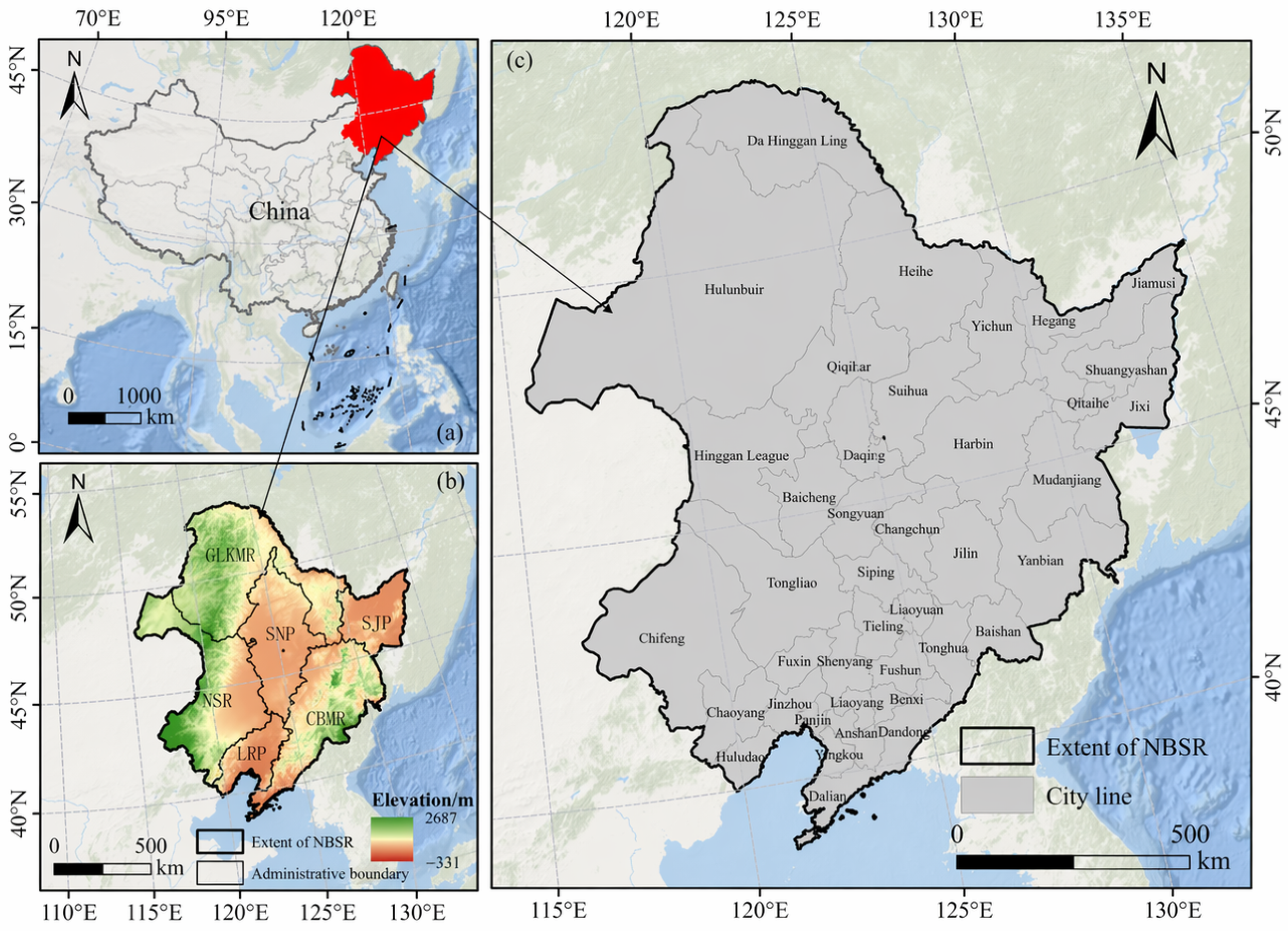
The Northeast Black Soil Region (NBSR) of China is one of the world’s four major black soil Regions. Located in northeastern China between 115°32′–135°09′ E and 38°42′–53°35′ N, it encompasses the entire Northeast region, including Heilongjiang Province, Jilin Province, Liaoning Province, as well as Hulunbuir City, Xing’an League, Tongliao City, and Chifeng City in eastern Inner Mongolia. The region spans a total land area of 1.2486 million km², characterized by a temperate continental monsoon climate with annual precipitation of approximately 500–600 mm and an average annual temperature of −5 to 4 °C. While rich black soil resources form the ecological foundation across the entire area, natural differentiation and human activities have combined to create six functional zones (Figure 1b), exhibiting a typical “mountains on three sides, central plains” pattern [20]. As China’s largest contiguous black soil belt and core commercial grain base, the Northeast Black Soil Region features expansive farmland suitable for large-scale agricultural production, primarily cultivating staple crops such as rice, corn, and soybeans. Population distribution in the Northeast Black Soil Region is uneven, concentrated primarily in urban centers and their surrounding areas, with cities like Harbin, Changchun, and Shenyang exhibiting high population densities. The entire region faces common ecological challenges including black soil degradation, water resource imbalance, and habitat fragmentation [21], forming a typical gradient space for analyzing the coupling mechanisms between ESs and HWB.

2.2. Data Sources

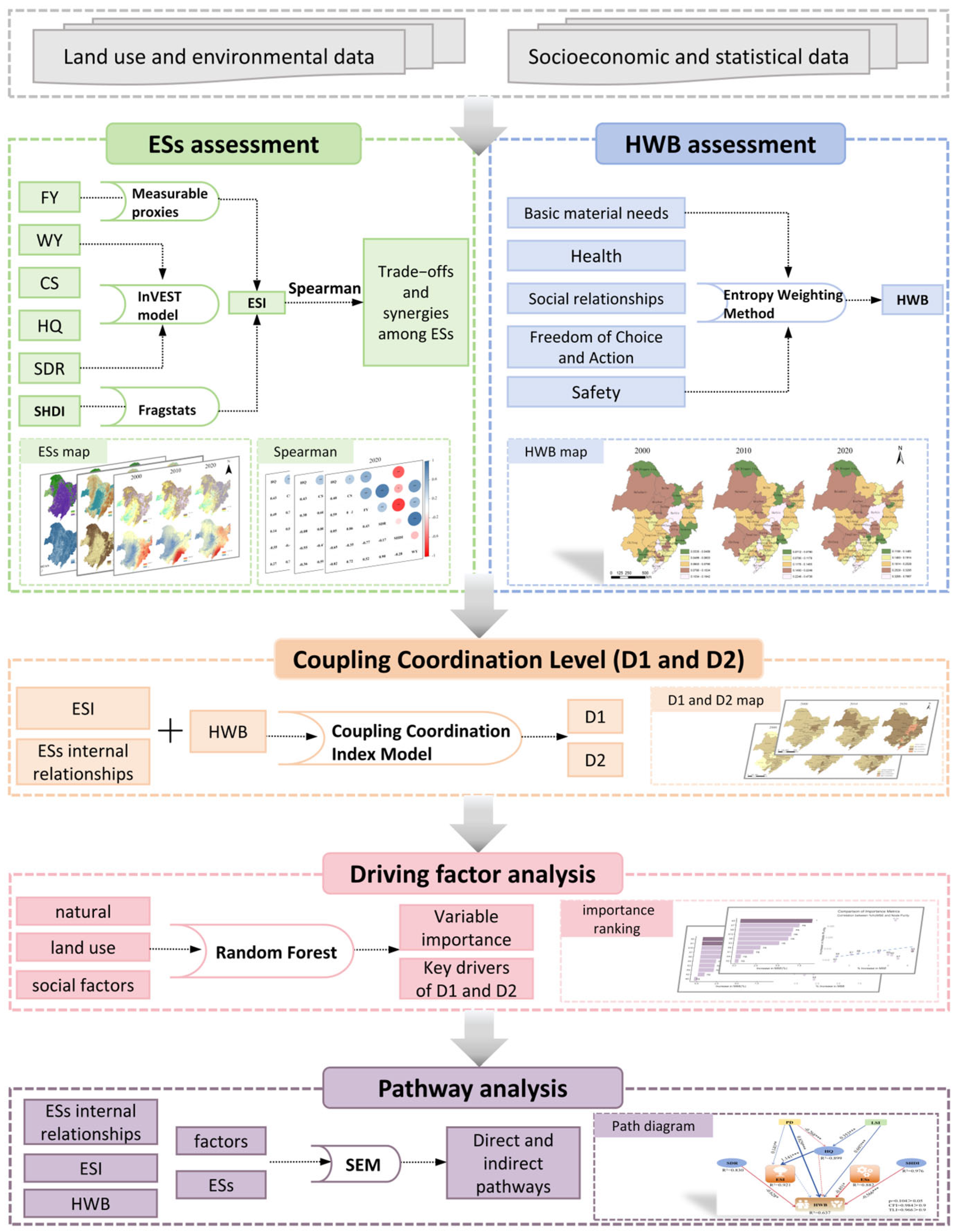
This study utilizes raster data and statistical information from 2000, 2010, and 2020 for model operations and indicator system calculations to quantify ecosystem services and assess human well-being.

Table 1. Data sources and information.

Data Type	Application Metrics	Data Format	Data Source
Land Use	HQ, SDR, WY, CS, SHDI, Driving factors (LSI, ED, CONTAG, LPI)	Raster	Resource Environment Science and Data Center
DEM	SDR	Raster
Precipitation	WY, SDR, Driving factors	Raster
NDVI	FY, SDR	Raster
Evapotranspiration	WY	Raster	National Ecosystem Science Data Center
Root depth, soil data	SDR, WY	Raster	China Soil Map Based on the Harmonized World Soil Database (HWSD)
Food production	FY	Sample	Statistical Yearbooks of Provinces and Municipalities, Bureau of Statistics
Socioeconomic Statistics	HWB, Driving factors	Sample
Population density	Driving factors	Raster	Worldpop
Air temperature	Driving factors	Raster	National Earth System Science Data Center
NPP	Driving factors	Raster	NASA Earth Science Data

lists the sources of all data used in this study. All raster data underwent standardization, resampling to a uniform spatial resolution of 1 km × 1 km, and conversion to the WGS_1984_Mercator projection coordinate system to meet model input requirements. Relevant statistical data were compiled from provincial and municipal Statistical Yearbooks. The overall methodological framework of this study is shown in Figure 2.

2.3. Ecosystem Services Assessment

Based on natural conditions, socioeconomic circumstances, and data availability, this study selected six key ecosystem services: Food yield (FY), Water yield (WY), Soil conservation (SDR), Carbon storage (CS), Habitat quality (HQ), and Shannon diversity index (SHDI) (

Table 2. Selection and evaluation of ecosystem services.

ES Level 1 Type	ES Level 2 Type	Calculation Method
Provision services	FY	Calculating using NDVI
	WY	InVEST (Annual Water Yield) Module
Regulation services	SDR	InVEST (Sediment Delivery Ratio) Module
	CS	InVEST (Carbon Storage and Sequestration) Module
Support services	HQ	InVEST (Habitat Quality) Module
Cultural services	SHDI	Calculated using Fragstats4.2 software

). These encompass all ecosystem service types within the Millennium Ecosystem Assessment classification framework [3]. The NBSR covers a vast area with complex and diverse land-use patterns, resulting in significant spatial variations in the provision of ecosystem services. As a technical tool supporting this study, the InVEST model, compared to other methods, is capable of providing relatively accurate and consistent quantitative assessments and spatial representations of ecosystem services across large scales, multiple time points, and various ecosystem service types, thereby establishing a unified data foundation for future research.

2.3.1. Food Yield (FY)

Food production refers to an ecosystem’s capacity to provide food resources for human consumption, serving as the foundation for human survival and development. To assess this region’s food production capacity, this study utilizes grain yield data and the NDVI index. Leveraging their linear relationship [22,23] and integrating land use data, we perform unit area allocation and calculation. Since construction land and unutilized land typically do not support food production, these land types were excluded for precise calculations. Only cultivated land, forest land, grassland, and water bodies were included in the analysis. Food production was aggregated based on the Statistical Yearbook, encompassing several categories: grains (rice, wheat, corn, sorghum, millet, tubers, soybeans, other coarse grains), vegetables, fruits, meat, poultry and eggs, dairy products, and aquatic products. The calculation formula is as follows [24]:

$$G_i= {\displaystyle \frac{NDV{I}_i}{NDV{I}_{sum}}} \times G_{sum}$$

(1)

where G_i represents the food yield allocated to raster; G_sum is the total food yield; NDVI_i is the NDVI value of raster; NDVI_sum is the total of NDVI values for cropland, forest land, grassland, and water bodies in the NBSR.

2.3.2. Water Yield (WY)

Water supply refers to an ecosystem’s capacity to provide usable water resources to humans and nature through precipitation, runoff, groundwater, and other means. In the Northeast Black Soil Region, this service plays a decisive role in agricultural irrigation and regional water security. The InVEST model calculates annual water yield through hydrological modeling, simulating how land cover types influence precipitation. It integrates factors such as precipitation and evapotranspiration, assessing each pixel’s water yield capacity based on distinct land-use and topographic characteristics. The biophysical table (CSV) required for this module is provided in Appendix A.1. The model Z parameter is set to 3.5 [25,26]. The calculation formula is as follows:

$$Y= \left(1 - {\displaystyle \frac{AET}{P}}\right) \times P$$

(2)

where Y is the annual water yield, and P and AET are the annual rainfall and actual evapotranspiration of raster x.

2.3.3. Soil Conservation (SDR)

SDR refers to an ecosystem’s capacity to maintain soil quality—including fertility and structural stability—by reducing erosion through vegetation cover and surface processes. Meanwhile, fertile, black soil regions are prone to degradation, making soil conservation services crucial for preventing desertification and safeguarding agricultural productivity [27]. Within the InVEST model, soil erosion impacts across different land-use types are simulated for assessment. This module employs the Universal Soil Loss Equation (USLE) to calculate soil erosion rates per pixel, thereby estimating soil conservation services. Biophysical characteristics are detailed in Appendix A.2 [28], with the calculation formula as follows:

$$SEDRE{T}_x = RKL{S}_x - USL{E}_x+SED{R}_x$$

(3)

$$RKL{S}_x=R_x\times K_x\times L{S}_x$$

(4)

$$USL{E}_x=R_x\times K_x\times L{S}_x\times C_x\times P_x$$

(5)

$$SED{R}_x=S{E}_x{\displaystyle \sum }_{y=1}^{x-1}USL{E}_y{\displaystyle \prod }_{z=y+1}^{x-1}\left(1-S{E}_z\right)$$

(6)

where SEDRET_x is the amount of soil and water conserved per unit x of the region; RKLS_x, USLE_x and SEDR_x are the natural erosion, the actual amount erosion, and the sediment retention; R_x, K_x and LS_x represent rainfall erosivity, soil erodibility, and slope length/gradient, respectively; C_X and P_X denote vegetation cover and management coefficients; SE_X is the interception rate; USLE_y is the actual amount of soil erosion in the upslope grid y; and SE_x is the amount of sediment intercepted.

2.3.4. Carbon Sequestration (CS)

CS in the black soil region refers to the ecosystem’s capacity to mitigate climate change by reducing atmospheric carbon dioxide levels through carbon fixation in vegetation and soil. The rich organic matter soils in the Northeast Black Soil Region confer significant carbon sink functions, holding strategic value for addressing climate change and achieving the “dual carbon” goals. The InVEST model accounts for carbon uptake and release processes across land types, estimating carbon storage per pixel based on biomass and soil carbon inventory calculation methods. Carbon density tables are presented in Appendix A.3 [29], with the calculation formula as follows:

$$CS = C_{above} + C_{above} + C_{dead} + C_{soil}$$

(7)

where CS is the total carbon stock, C_above and C_below are the above-ground and below-ground carbon stocks, C_dead represents dead organic matter, and C_soil represents soil carbon.

2.3.5. Habitat Quality (HQ)

As a transitional zone between agriculture and natural ecosystems, the Northeast Black Soil Region’s habitat quality directly impacts biodiversity conservation and ecosystem stability [30]. The assessment principle of this InVEST model module is based on an ecosystem’s ability to support biodiversity and habitats. The habitat quality index reflects the quality of habitat provided by ecosystems within a specific area. A higher habitat quality index indicates stronger support capacity for species habitats in that region [31]. This study adopts a Z-value of 0.05. Sensitivity and biophysical threat sources are detailed in Appendix A.4 and Appendix A.5 [32]. The calculation formula is as follows:

$$Q_{xj} = H_j\left[1 - ({\displaystyle \frac{D_{xj}^z}{D_{xj}^z + k^2}})\right]$$

(8)

$$D_{xj}={\displaystyle \sum }_{r=1}^R{\displaystyle \sum }_{y=1}^{Y_r}{r}_y\left({\displaystyle \frac{{\delta }_r}{{{\displaystyle \sum }}_{r=1}^R{\delta }_r}}\right)\left[1-{\displaystyle \frac{d_{xy}}{d_{rmax}}}\right]{\lambda }_x{S}_{jr}$$

(9)

where (1) Q_xj is the habitat quality value; H_j is the habitat suitability; k is the half-saturation constant; z is the normalization constant, which is taken as 0.05 in this study; and D_xj is the habitat degradation index. (2) R is the number of stress factors; r_y, δr are the disturbance degree and weight of the region where the threat source is located; λ_x, S_jr are the anti-disturbance ability and sensitivity of the raster unit, respectively; Y_r is the number of rasters of the threat factor; and d_xy, d_rmax are the Euclidean distance between the threat source and the regional unit and the maximum radius of disturbance, respectively.

2.3.6. Shannon Diversity Index (SHDI)

SHDI is a commonly used metric for measuring species diversity within ecosystems or landscapes. At the landscape level, it can also indirectly reflect the impact of landscape diversity on cultural services. Therefore, in cultural service assessments—particularly when cultural services depend on the diversity of natural landscapes—the Shannon diversity Index can serve as a method for evaluating cultural services [33]. A higher SHDI indicates greater richness in landscape types. The calculation formula is as follows:

$$H = -{{\displaystyle \sum }}_{i=1}^S{p}_{i \times ln\left(p_i\right)}$$

(10)

where H is Shannon diversity index value; p_i is the proportion of the ith landscape type.

2.3.7. Ecosystem Service Index Calculation (ESI)

The values of FY, CS, WY, SDR, HQ, and SHDI exhibit significant differences in magnitude. Based on this, this study standardized the results for the six ecosystem services by converting ES values to a dimensionless scale of [0, 1]. Fuzzy membership functions in ArcGIS10.8.1 were used for normalization to eliminate differences between indicators. Subsequently, spatial overlay with equal weights was performed to calculate the composite value ESI, facilitating subsequent computational and comparative analysis.

2.4. Human Well-Being Assessment

This study constructs an indicator system based on the human well-being assessment framework proposed in the Millennium Ecosystem Assessment report [3]. It encompasses five dimensions—“basic material needs, security, health, good social relationships, and freedom of choice and action”—to reflect the multi-level structure of human well-being. Among these, basic material needs emphasize the material foundations necessary for humans to maintain a decent standard of living; health primarily reflects the ability to maintain physical well-being, access basic medical services, and enjoy good living conditions; positive social relationships involve not only stable family ties but also social support and basic security; freedom of choice and action primarily reflects an individual’s capacity for development in areas such as education, resource accumulation, and opportunities for advancement, and indicates the potential to improve one’s life and achieve long-term development; and security primarily reflects residents’ ability to withstand risks and their level of basic protection in terms of resource ownership, livelihood security, and employment stability. Together, these five dimensions constitute the comprehensive essence of human well-being and can systematically reflect differences in the living conditions and development opportunities of residents across regions.

The establishment of this indicator system primarily focuses on quantifying objective well-being, i.e., conducting assessments using accessible and verifiable statistical data and socioeconomic data [34]. Priority was given to statistical indicators from 40 prefecture-level cities in the NBSR at the three time points of 2000, 2010, and 2020 that demonstrated good availability, continuity, and comparability, in order to ensure the feasibility and consistency of long-term time series analysis and large-scale regional comparisons. In contrast, assessments of subjective well-being often rely on questionnaire surveys and perceived data [35], exhibiting significant subjectivity and regional variability, making it challenging to obtain stable data across large scales and long time series. Therefore, this study exclusively employs objective well-being indicators for evaluation to ensure the scientific rigor and comparability of the assessment results.

In determining the indicator weights, this study employed the entropy weighting method to assign weights to each indicator. The resulting weights for each indicator are presented in

Table 3. Selection of Human Well-Being indicators. “+” indicates a positive indicator; “−” indicates a negative indicator.

Primary Indicators	Secondary Indicators	Direction	Unit	Weight
Basic material needs	Per capita gross domestic product	+	CNY	0.0676
	Per capita crop yield	+	t/capita	0.0955
Health	Number of beds in healthcare institutions	+	pcs	0.0804
	Number of personnel in healthcare institutions	+	persons	0.0810
Social relationships	Number of divorces per year	−	pairs	0.0056
	Social Security and Employment Expenditure	+	104 CNY	0.1280
Freedom of Choice and Action	Education expenditure	+	104 CNY	0.1075
	Number of students enrolled in higher education institutions	+	persons	0.2125
	Year-end balance of savings deposits at resident financial institutions	+	104 CNY	0.1438
Safety	Per capita arable land area	+	kha/104 persons	0.0691
	Registered urban unemployed persons	−	persons	0.0091

. This method determines weights based on the variability of indicators, thereby mitigating the direct impact of subjective weighting to some extent and enhancing the consistency of multi-indicator comprehensive evaluations. Ultimately, the comprehensive calculation yielded the Human Well-Being Index for each city within the study area, serving to characterize the overall level of HWB and its spatial differentiation patterns across the region. It should be noted that the entropy weighting method reflects differences in the information content of indicators rather than their absolute importance in ecological or socioeconomic terms; therefore, its results are more suitable for regional comparative analyses conducted on a large scale and over long time series.

2.5. Calculation of the Landscape Index

This study incorporated landscape pattern factors into its analysis of driving factors and mechanisms. Using 2020 land-use data and classifications from the NBSR, the Landscape Shape Index (LSI), Largest Patch Index (LPI), Edge Density (ED), and Contagion Index (CONTAG) were calculated at the landscape level using Fragstats software. The formulas are as follows:

(1) LSI: This index measures the complexity of the shape of land cover patches. It ranges from 0 to 1; the higher the value, the more complex the shape of the patch and the longer its perimeter. Here, P represents the perimeter of the patch, and A represents its area.

$$\mathrm{LSI}={\displaystyle \frac{\mathrm{P}}{\sqrt{\mathrm{A}}}}$$

(11)

(2) LPI: This index helps identify the dominant or predominant types present in a landscape. Its value determines ecological characteristics such as the abundance of dominant and subordinate species within the landscape. The index ranges from 0 to 100, where A_ij represents the area of a single patch of a given landscape type.

$$\mathrm{LPI}={\displaystyle \frac{{\mathrm{Max}}_{\mathrm{j}=1}^{\mathrm{n}}{\mathrm{A}}_{\mathrm{ij}}}{\mathrm{A}}}\times 100$$

(12)

(3) ED: Refers to the total length of a patch’s edges per unit area. It reflects the degree of fragmentation of the patch’s boundaries; the higher the value, the more complex the boundaries, the greater the irregularity, and the stronger the capacity for material exchange. E represents the total length of all edges, and A represents the total area of the landscape.

$$\mathrm{ED}={\displaystyle \frac{\mathrm{E}}{\mathrm{A}}}\times \mathrm{10,000}$$

(13)

(4) CONTAG: This index is a measure of landscape connectivity and is commonly used to describe the degree of clustering among different landscape classes within a landscape. Its range is from 0 to 100, where p_ij represents the transition probability between landscape classes i and j; n is the number of landscape classes.

$$\mathrm{CONTAG}=[1+{\displaystyle \sum }_{\mathrm{i}=1}^{\mathrm{m}}{\displaystyle \sum }_{\mathrm{j}=1}^{\mathrm{n}}{\displaystyle \frac{{\mathrm{P}}_{\mathrm{ij}}\ln \left({\mathrm{P}}_{\mathrm{ij}}\right)}{2\ln \left(\mathrm{m}\right)}}]\left(100\right)$$

(14)

2.6. Data Analysis

To systematically elucidate the characteristics of the relationship between ESs and HWB in the NBSR, as well as the mechanisms underlying this relationship, this study first employs Spearman’s correlation analysis to identify trade-offs and synergies among various ESs, based on a quantitative assessment of both. Second, a coupling coordination model is employed to characterize the coordination relationships between the total supply of ESs, the internal balance of ESs, and HWB, respectively. Subsequently, a random forest model is used to identify the key drivers of these two types of coupling relationships. Finally, structural equation modeling is utilized to analyze the causal pathways among the primary factors. These methods are sequentially integrated and mutually complementary, collectively identifying and explaining the interactive relationships between ESs–HWB.

(1) Coupling Coordination Index Model: The coupling coordination index serves as a metric for evaluating the interaction, coordination level, and developmental state between two systems. In this study, it is employed to quantify the interrelationship between the ESs index and HWB index, reflecting their coordinated development level [36]. Results closer to 1 indicate stronger coordination, while values near 0 suggest poor alignment. Based on the coupling coordination degree model results and prior research, coupling stages and coordination levels were defined (

Table 4. Coupling coordination level classification.

Coupling Level		Coupling Coordination Level
Coupling Degree	Coupling Stage	Coupling Coordination Degree	Coordination Level
0 < C ≤ 0.4	Low-level coupling	0 < D ≤ 0.4	Severe imbalance
0.4 < C ≤ 0.6	Antagonistic coupling	0.4 < D ≤ 0.6	Mild imbalance
0.6 < C ≤ 0.8	Break-in coupling	0.6 < D ≤ 0.8	Good coordination
0.8 < C ≤ 1.0	High-level coupling	0.8 < D ≤ 1.0	High coordination

) to characterize the coupling patterns between ecosystem services and human well-being [37]. The calculation formula is as follows:

$$C= {\displaystyle \frac{2\sqrt{ES\times HW}}{ES+HW}}$$

(15)

$$T=\alpha \times ES+\beta \times HW$$

(16)

$$D=\sqrt{C\times T}$$

(17)

where ES denotes the Ecosystem Services Index; HWB denotes the Human Well-Being Index; C denotes the coupling degree; T denotes the coordination index; D denotes the coupling coordination degree; and α and β are the comprehensive coordination evaluation coefficients, which are considered equally important in this study and set to 0.5 respectively.

(2) Spearman’s Rank Correlation Coefficient: Spearman’s correlation analysis is a nonparametric statistical method used to assess monotonic relationships between variables without requiring linearity or normal distribution. In this study, Spearman’s correlation analysis was employed to examine trade-offs and synergies among different ecosystem services. When p < 0, a trade-off relationship exists; when p > 0, a synergistic relationship is present [38]. The calculation formula is as follows:

$$p =1 -{\displaystyle \frac{6\sum d_i^2}{n\left(n^2-1\right)}}$$

(18)

where di is the difference between the orders of two variables in the i-th sample; n is the sample size.

(3) Random Forest (RF) [39]: To analyze the drivers and contribution levels of ESs and HWB, this study employed a random forest model based on permutation tests. Random forest is an ensemble learning technique that enhances prediction accuracy and stability by constructing multiple decision trees and aggregating their outputs. Unlike classical methods, this study core employs the R4.3.3 package “rfPermute,” which implements random forest modeling while incorporating built-in repeated permutation testing to directly assess the statistical significance of each driver’s importance metric. The “caret” package was used for data partitioning and model preprocessing, the “randomForest” package provided the foundational algorithm support, the “pdp” package was employed to construct partial dependence plots, and “ggplot2” along with related extension packages completed the visualization of results, ensuring the model’s integrity and intuitiveness.

(4) Structural Equation Modeling (SEM) [40]: To investigate the specific pathways and mechanisms linking ESs to HWB, this study employs structural equation modeling. This method simultaneously assesses causal relationships among multiple sets of variables and the overall model fit, revealing key pathways and mechanisms through standardized path coefficients and their significance levels. Model construction and testing were implemented using the “lavaan” package in R. Model fit was assessed using chi-square test p-values and Comparative Fit Index (CFI) values, where p > 0.05 and CFI values closer to 1 indicate better model fit.

3. Results

3.1. Analysis of Changes in Ecosystem Services

3.1.1. Spatio-Temporal Variations in Ecosystem Services

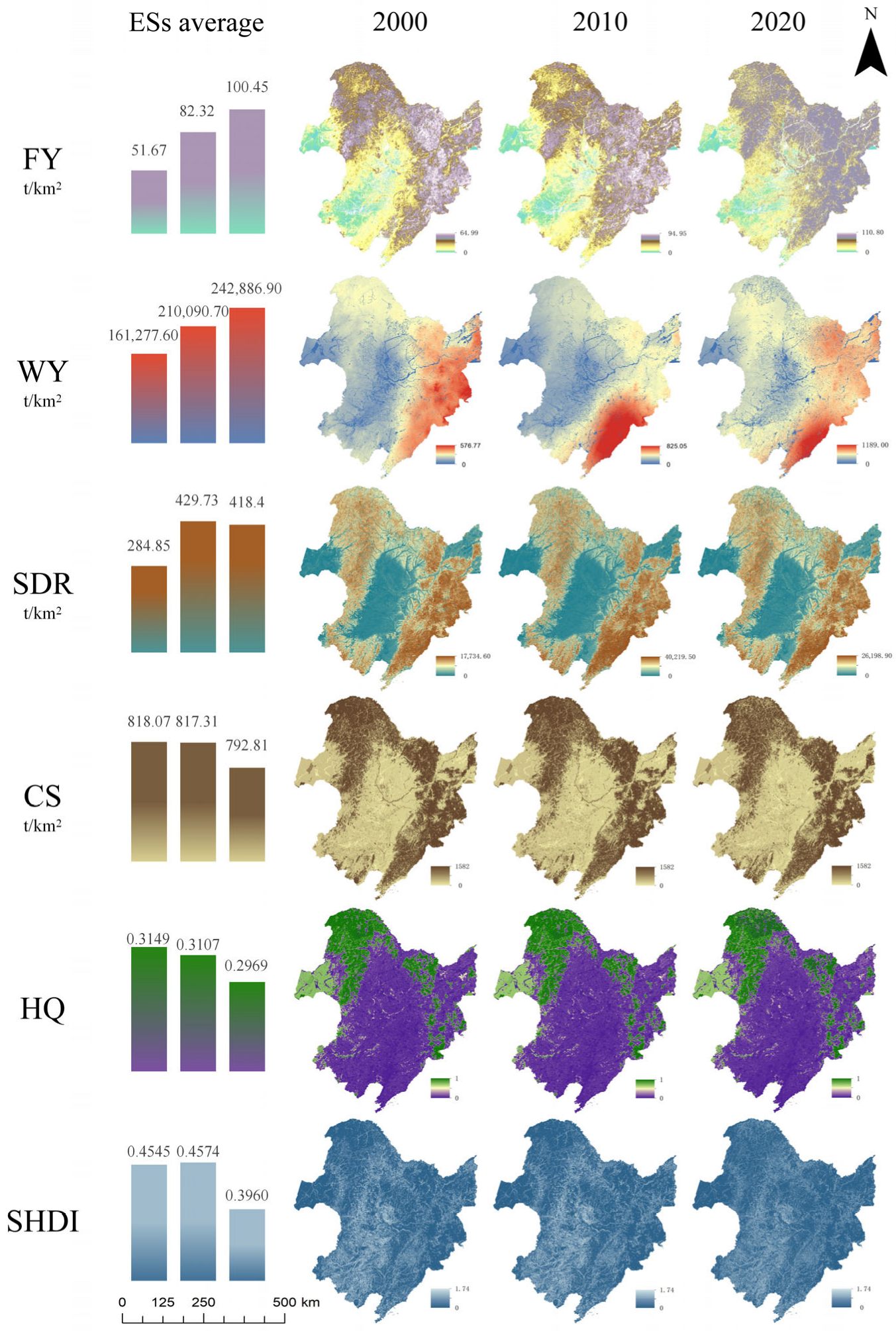
Results indicate that NBSR exhibited significant spatial heterogeneity between 2000 and 2020 (Figure 3). Spatially, FY showed pronounced Regional differentiation, with high-value areas concentrated in the southern Greater and Lesser Khingan Ranges, the Sanjiang Plain, and the Changbai Mountain region, while low-value areas were predominantly distributed in the northwestern wind-sand zone. WY follows a spatial distribution pattern of “higher in the southeast, lower in the northwest, decreasing from east to west,” which largely aligns with the spatial distribution of precipitation. CS and SDR exhibit similar spatial patterns, characterized by “higher values in mountainous areas and lower values in plains,” with relatively small interannual fluctuations. HQ high-value areas are concentrated in mountainous regions such as the Greater and Lesser Khingan Ranges, while SHDI shows an opposite spatial pattern.

From a temporal perspective, significant divergence in indicators was observed throughout the study period. Specifically, FY and WY showed substantial increases, rising by 94.41% (from an average of 51.67 t/km² to 100.45 t/km²) and 50.60% (from an average of 161,277.6 m³/km² to 242,886.9 m³/km²), respectively. CS and HQ decreased by 3.09% and 5.72%, respectively. SDR and SHDI exhibited an initial increase followed by a decline. However, SDR showed a net increase of approximately 46.88% during the study period, while SHDI exhibited a net decrease, dropping from 0.4545 to 0.3960, representing a reduction of about 12.87%.

3.1.2. Spatio-Temporal Variations in Ecosystem Services Index (ESI) at the Municipal Level

Overall, from 2000 to 2020, the ecological sustainability (ES) level of the Northeast China Border Region (NBSR) showed an initial upward trend followed by a decline. A distinct phase transition occurred around 2010, with the 2020 ES level slightly lower than that of 2000. This indicates a certain degree of degradation in the regional ES status over the past decade, a trend consistently reflected in the Ecological Sustainability Index (ESI) (Figure 4). At the city level, the spatial pattern of the ESI remained relatively stable, with high-value areas consistently concentrated in the Greater Khingan Range and Hulunbuir regions, which possess favorable ecological foundations. Between 2000 and 2010, spatial changes in low-value ESI zones were relatively limited, primarily distributed across regions dominated by agricultural development and urban construction, such as Qiqihar, Suihua, Daqing, Baicheng, Songyuan, Changchun, Shenyang, Panjin, and Jiamusi. After 2010, ESI values showed a certain rebound in some cities (such as Changchun, Songyuan, Siping, and Shenyang), while others experienced minor fluctuations. This indicates that, against the backdrop of an overall decline in ES, different cities exhibit distinct responses to ecosystem changes.

3.1.3. Trade-Offs and Synergies in Ecosystem Service Functions

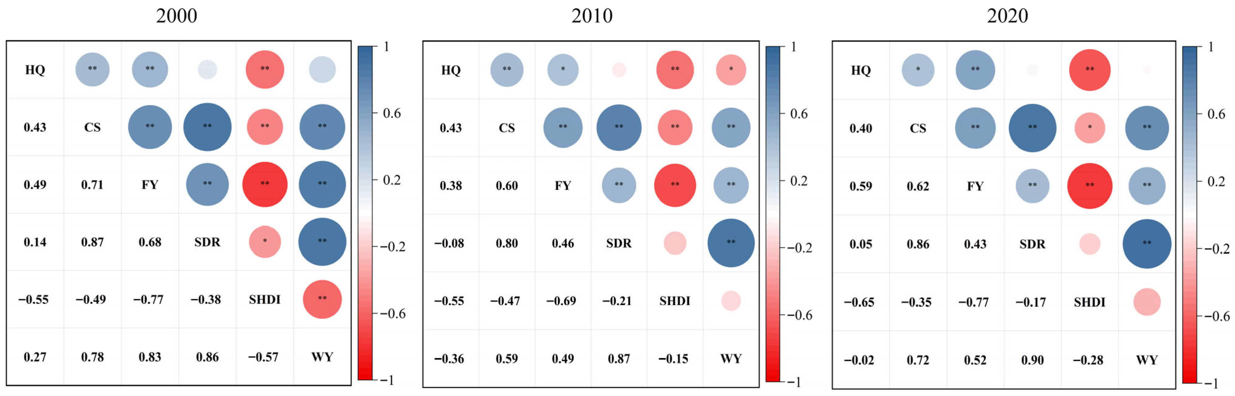
This study identified 15 correlations among six ESs over a three-decade period. Significant correlations were observed in 13, 12, and 11 pairs in 2000, 2010, and 2020, respectively (p < 0.05), indicating widespread synergistic and trade-off relationships among ESs (Figure 5). Regarding synergistic relationships, CS, SDR, and WY consistently maintained significant positive correlations, which strengthened from 2010 to 2020 while remaining at high levels overall, reflecting strong coordination among regulatory services. The correlation between FY and HQ first declined then increased, reaching its strongest synergistic relationship in 2020. Regarding trade-offs, notably, SHDI exhibited persistent trade-offs with the other five ESs throughout the three-year period. In 2010, significant trade-offs between SHDI and FY/HQ remained, though its negative correlations with SDR and WY had moderated compared to 2000. This indicates a trend toward reduced conflicts between landscape patterns and certain regulating services, yet SHDI’s constraints on provisioning services and habitat quality persist. Overall, synergistic relationships among most ESs have strengthened over the past two decades, particularly with increasing correlations among regulating services. Meanwhile, landscape pattern changes represented by SHDI remain the primary factor constraining the overall synergistic enhancement of regional ESs.

3.2. Analysis of Spatio-Temporal Changes in Human Well-Being

3.2.1. Spatial Variation Analysis of Human Well-Being

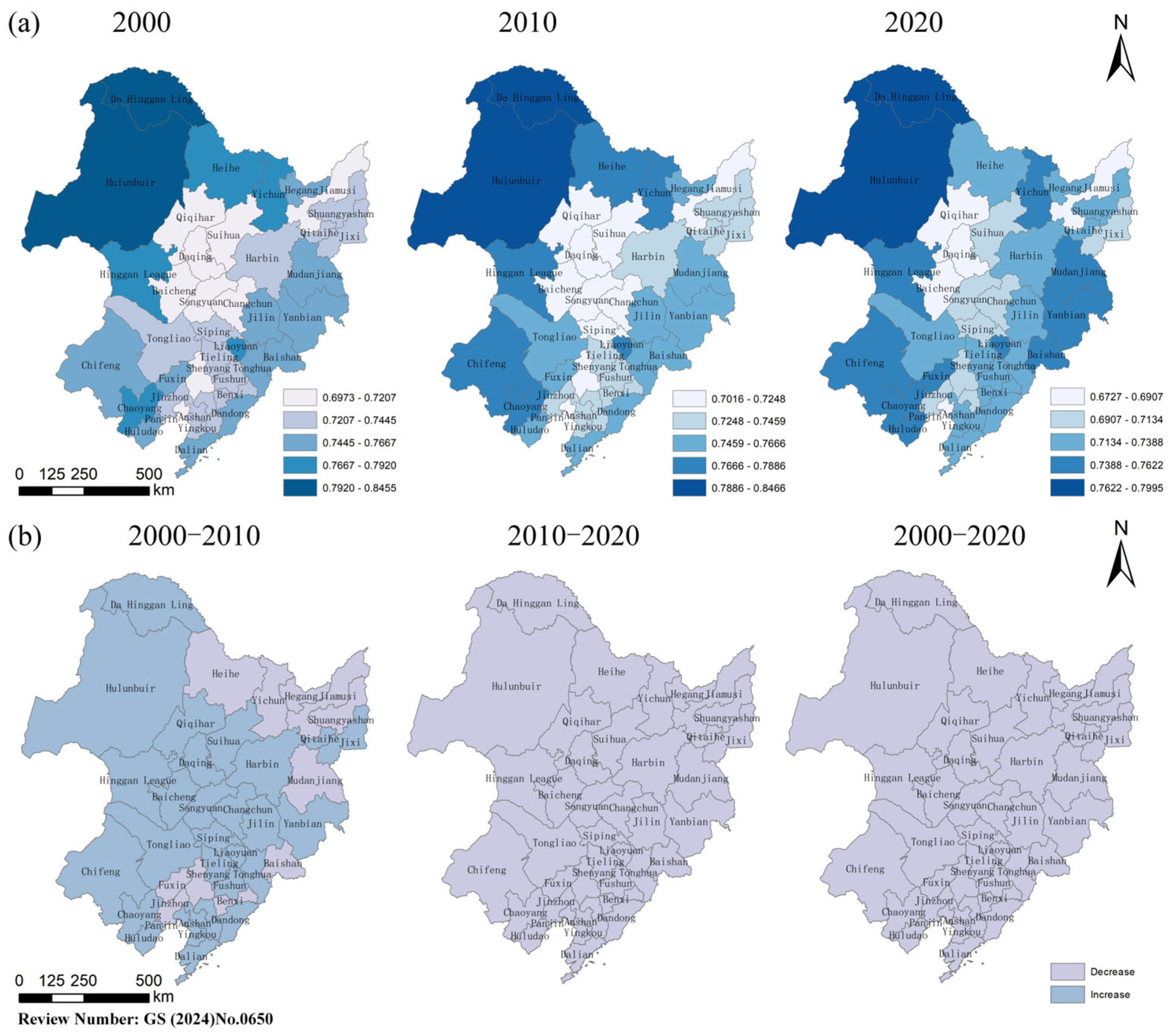
During the years 2000, 2010, and 2020, the HWB levels across cities in the Northeast Black Soil Region exhibited significant spatial variations while maintaining a relatively stable overall pattern (Figure 6). During the study period, cities with high HWB scores were primarily concentrated in core regional cities and provincial capitals. Shenyang, Changchun, Harbin, and Dalian consistently led the rankings, achieving scores of 0.75, 0.67, 0.77, and 0.62 respectively in 2020. In contrast, Da Hinggan Ling, Qitaihe, and Baishan City scored low across all three time points, maintaining persistently low HWB levels over the long term.

From a temporal perspective, cities such as Chaoyang, Liaoyuan, Yichun, and Yanbian saw improvements in their HWB levels between 2000 and 2020, though overall levels remained relatively low. Other cities experienced minor fluctuations within the medium-to-high range, without significant shifts in tier classification. Overall, disparities in HWB levels among cities in the Northeast Black Soil Region persisted throughout the study period. A cluster of cities with high HWB levels, represented by Harbin, Dalian, Shenyang, and Changchun, gradually stabilized and took shape.

3.2.2. Analysis of Human Well-Being over Time

From a temporal perspective, the HWB levels of all NBSR cities showed continuous improvement during the study period, though growth rates varied significantly, leading to widening disparities within the region. Harbin, Shenyang, Changchun, and Dalian demonstrated the most pronounced increases (Figure 7), averaging approximately 318.14% growth over two decades and consistently maintaining priority development status. By time period: Between 2000 and 2010, cities with the smallest increases included Greater Khingan Range, Yichun, Hegang, Qitaihe, and Huludao, averaging approximately 69.45% growth, predominantly concentrated in Heilongjiang Province; from 2010 to 2020, the cities with the lowest growth rates were Greater Khingan Range, Daqing, Fuxin, Fushun, Liaoyuan, and Baishan, averaging approximately 41.01%. Overall, cities with the lowest HWB scores in each period also generally exhibited the smallest growth rates, further entrenching the low-level development pattern of lagging cities.

3.3. Analysis of the Relationship Between Ecosystem Services and Human Well-Being

3.3.1. Spatial Differentiation of ESI-HWB Coupling Coordination Degree (D1)

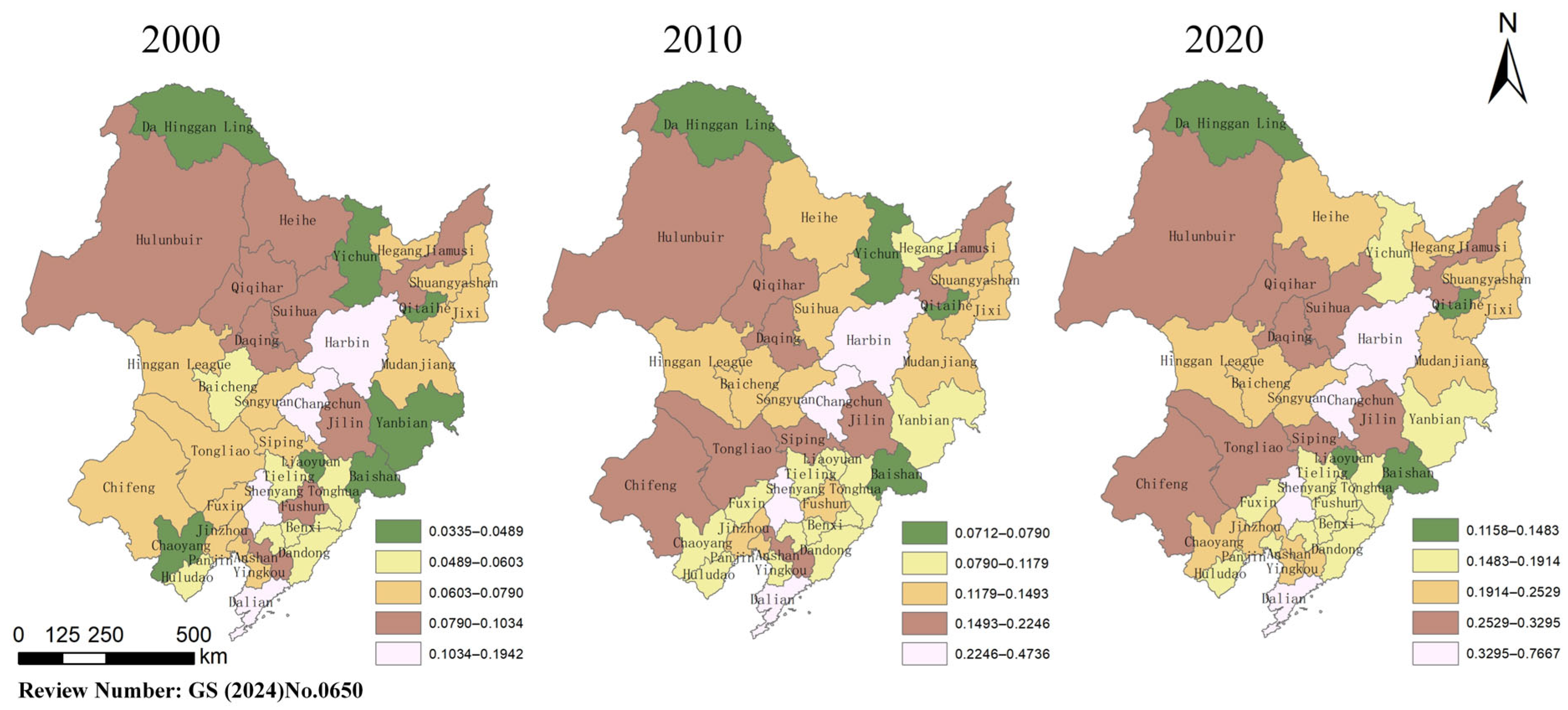
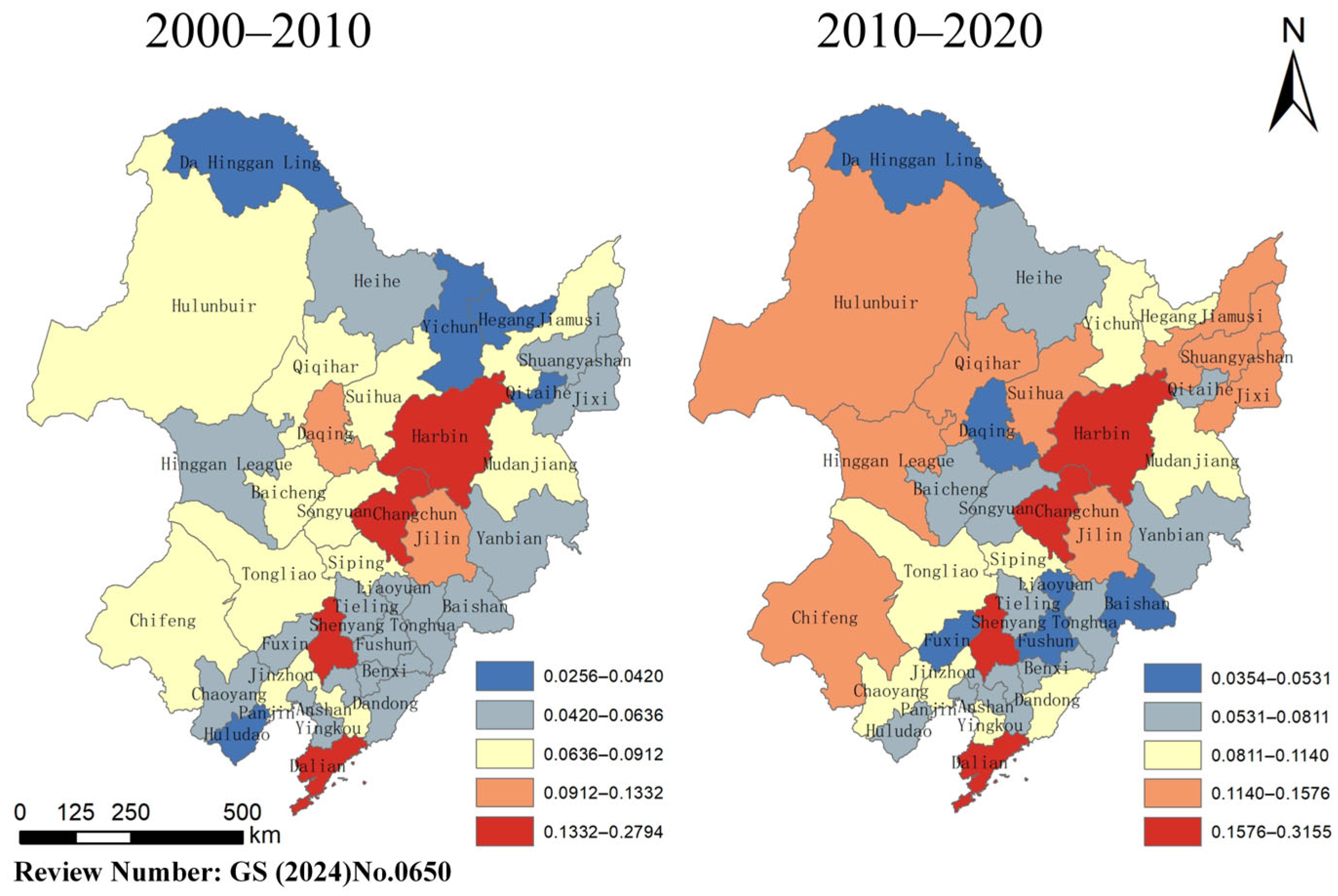
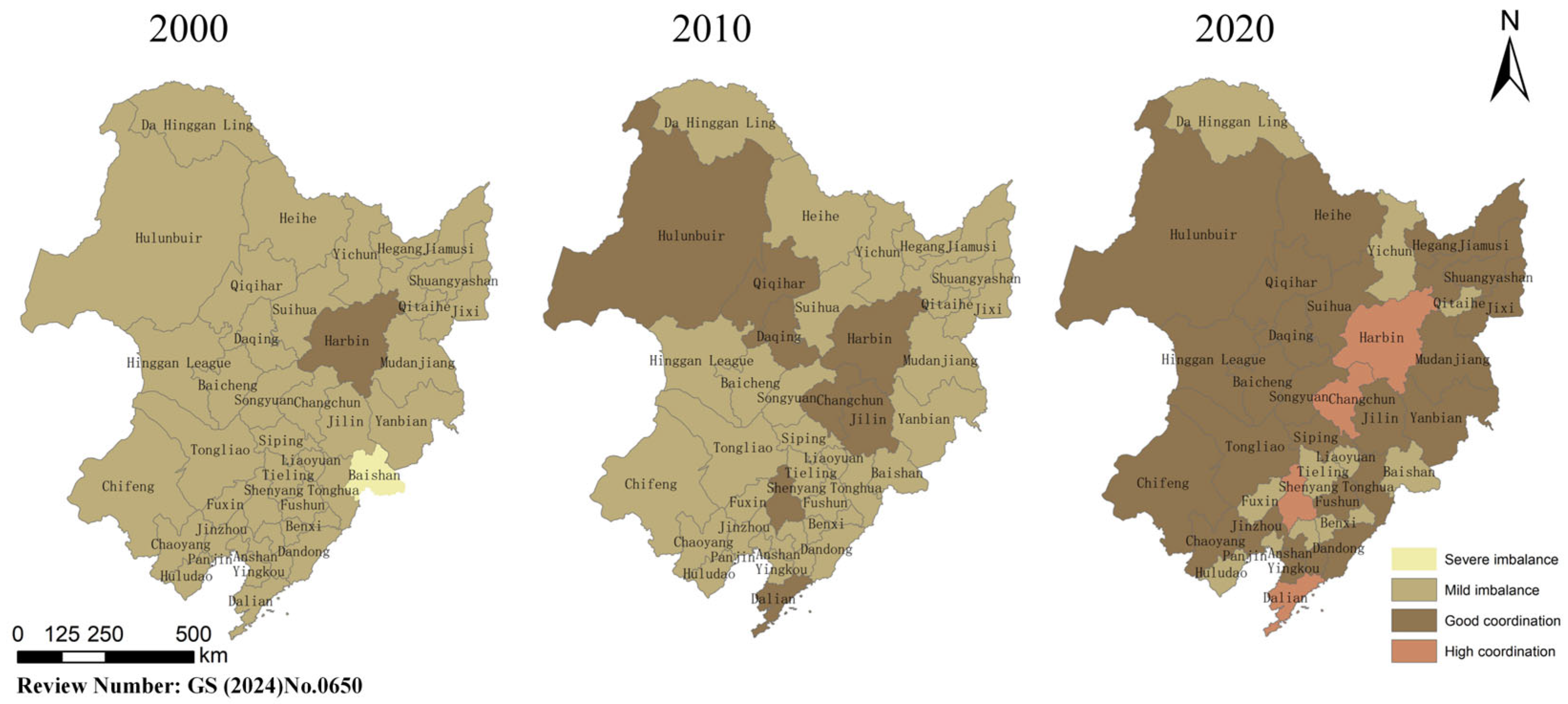
During the study period, the level of coordination between ESI and HWB in the Northeast Black Soil Region continued to improve (Figure 8). In 2000, the overall regional coordination level remained relatively low, with 38 out of 40 cities classified as having a mildly imbalanced status. By 2010, regional coupling coordination began to improve significantly. The number of cities achieving a well-coordinated level increased from 1 in 2000 to 8, primarily concentrated in Hulunbuir, Qiqihar, Daqing, Harbin, Changchun, Jilin, Shenyang, and Dalian. While the remaining cities remained in a mildly imbalanced state, their coupling coordination values showed varying degrees of improvement. By 2020, most cities transitioned from imbalance to coordination levels, achieving a cross-stage improvement in regional ESI-ESs coupling coordination. Among them, core cities like Harbin, Changchun, Shenyang, and Dalian attained high coordination levels, exhibiting strong consistency between their spatial distribution patterns and high-value HWB zones.

3.3.2. Spatial Differentiation of Coupling Coordination Degree (D2) Between the Coupling Coordination Degree Among Various ESs and the Human Well-Being Index

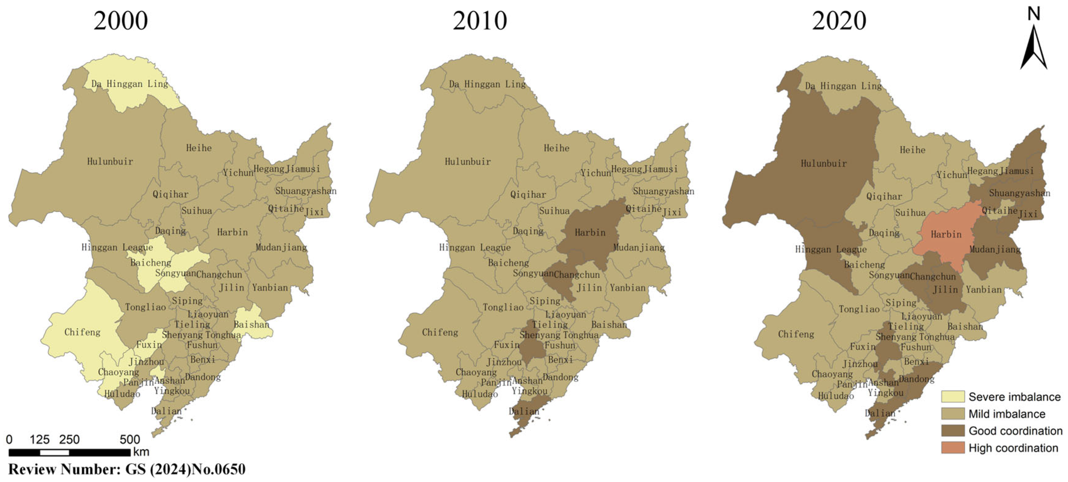
Based on the statistical results of six ecosystem services at the city scale, we further calculated the coupling coordination degree among internal functions of ESs and conducted a coupling analysis with the human well-being index. This yielded the coupling coordination degree (D2) between the internal coordination of ESs and HWB (Figure 9). Over the 20-year period, D2 showed an overall upward trend, yet its coupling coordination level remained weaker than D1, indicating that the coordination within the functional structure of ecosystem services remains a key factor constraining regional comprehensive coupling levels. From a temporal perspective, all cities exhibited severe or mild coordination deficits in D2 in 2000, revealing widespread coordination deficiencies among ecosystem service functions. By 2010, core cities like Harbin, Changchun, Shenyang, and Dalian transitioned from coordination deficits to good coordination levels, while other cities, though still mildly deficient, showed improved coupling coordination indices. By 2020, Harbin’s D2 further improved to a highly coordinated level, while other cities showed varying degrees of growth in coupling coordination. However, most cities remained at a mildly uncoordinated level. Compared to D1, D2 exhibited significant lag in overall coordination levels and the magnitude of level transitions, further highlighting the critical constraining role of coordination among internal ecosystem service functions on regional ES–HWB integrated coupling levels.

3.4. Drivers of the Coupling Relationship Between Ecosystem Services and Human Well-Being

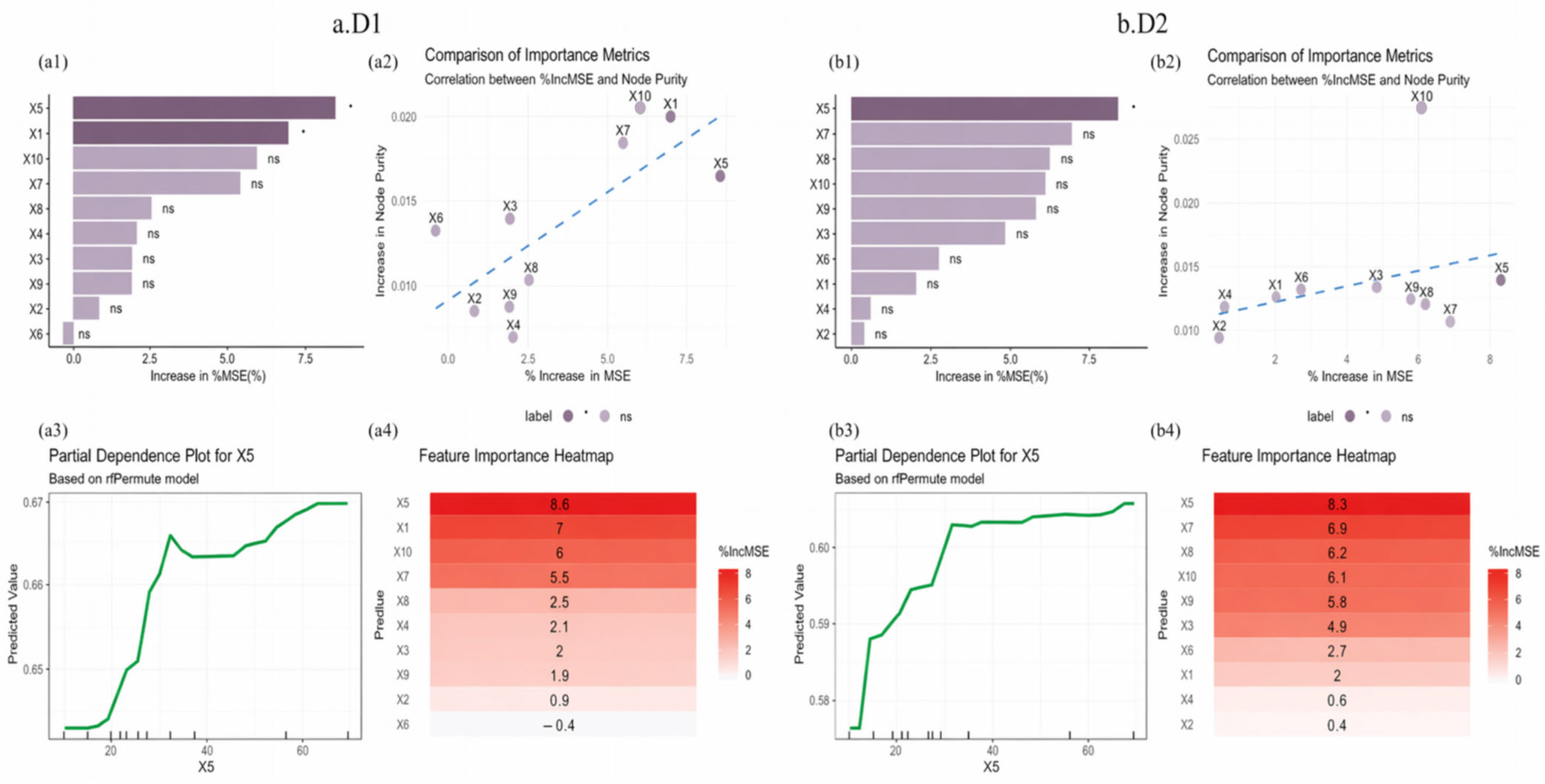
To reveal the primary drivers of the coupling relationship between ESs and HWB in the Northeast Black Soil Region, this study conducted separate driver analyses for two coupling coordination indices (D1 and D2). Considering regional conditions, ten indicators across natural, land use, and social factors were selected for quantitative assessment in 2020. Natural factors included temperature (Temp, X1), precipitation (Pre, X2), net primary productivity (NPP, X3), and elevation (DEM, X4); land-use factors were represented by landscape indices, including Landscape Shape Index (LSI, X5), maximum patch index (LPI, X6), edge density (ED, X7), and contiguity index (CONTAG, X8). Social factors comprised urbanization rate (Urb, X9) and population density (PD, X10).

The results of the driving factor analysis (Figure 10 and

Table 5. Random forest analysis results. RMSE denotes root mean square error; R² denotes coefficient of determination; MAE denotes mean absolute error.

	RMSE	R2	MAE
D1	0.0672	0.4935	0.0466
D2	0.0437	0.2029	0.0347

) reveal that for indicator D1, changes in coupling coordination are jointly dominated by three dimensions, indicating that coordination from the total supply perspective arises from the integrated effects of all dimensions. The top three contributing factors are LSI (X5), Temp (X1), and PD (X10), with LSI and Temp exhibiting significant influence. The partial dependency plot reveals that as LSI values increase, the predicted value of D1 first rises rapidly before stabilizing, indicating that heightened landscape complexity promotes coordination in total supply. In contrast, the driving mechanism for D2 changes, with land-use factors significantly strengthening their influence. The top three contributors are all landscape indicators: LSI (X5), ED (X7), and CONTAG (X8), with LSI exhibiting significance. This indicates that from an internal coupling coordination perspective, landscape plays a crucial and non-negligible role. Meanwhile, the influence of social factors (X9, X10) and Temp (X1) in the D2 model has diminished. Additionally, Pre (X2) and DEM (X4) exhibit low and insignificant contribution rates in both models, suggesting that topography and moisture conditions provide relatively limited explanatory power for coupling coordination at the scale of the NBSR.

Overall, from the perspective of total supply and internal coupling coordination, landscape pattern factors demonstrated overwhelming explanatory power. Notably, the Landscape Shape Index (X5) emerged as a common core significant factor in both models. This indicates that optimizing landscape spatial configuration and enhancing landscape complexity and integrity represent key pathways to elevate the coupling level between ESs and HWB in the NBSR.

3.5. Pathways of Influence for Various Factors

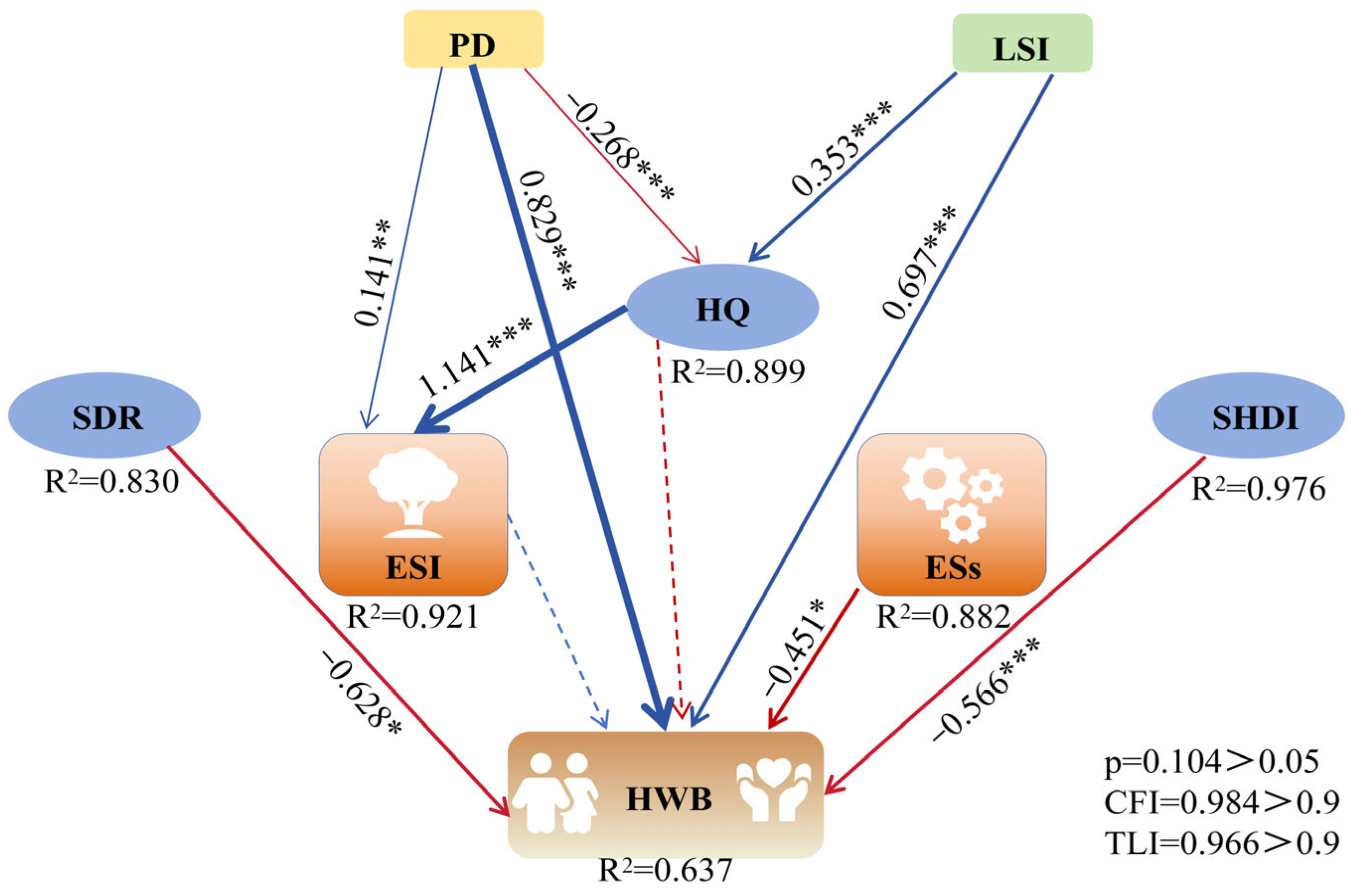
To further clarify the pathways through which various drivers influence ESs and HWB, this study constructed a Structural Equation Model (SEM). Model fit results (p = 0.104 > 0.05, CFI = 0.984 > 0.9, TLI = 0.966 > 0.9) indicate the model possesses good explanatory power. The SEM results strongly support the findings from the random forest analysis and further reveal the pathways through which landscape patterns influence various ESs and HWB. The model indicates that all 10 factors can affect HWB by influencing ecosystem services, with specific values presented in Appendix A.6.

The Landscape Shape Index (LSI) and Population Density (PD) directly influence HWB, as shown in Figure 11. Specifically, LSI not only significantly promotes HWB directly (β = 0.697, p < 0.001) but also exhibits a distinct mediating effect. LSI positively drives habitat quality (HQ) (β = 0.353, p < 0.001), thereby indirectly enhancing total ecosystem service provision (ESI) (β = 1.141, p < 0.001) and ultimately exerting a positive influence on HWB. This indicates that optimizing landscape spatial configuration is a critical entry point for enhancing regional well-being in the NBSR. The socioeconomic factor PD directly enhances HWB (β = 0.829, p < 0.001) but exerts a significant negative impact on HQ, revealing the potential threat of human activity concentration to ecosystem stability.

As shown in Appendix

Table A6. SEM of coupling coordination among ESs, Factors, ESI, and HWB. “*” indicates p < 0.05, “**” indicates p < 0.01, “***” indicates p < 0.001.

Response	Predictor	Estimate	p	Sig
ESs	Temp	−0.253	0.001	***
ESs	Pre	0.357	0.000	***
ESs	CONTAG	−0.281	0.000	***
ESs	CS	0.804	0.000	***
ESI	Temp	0.267	0.001	**
ESI	Pre	−0.962	0.000	***
ESI	DEM	0.187	0.001	***
ESI	ED	0.512	0.000	***
ESI	Urb	−0.173	0.002	**
ESI	PD	0.141	0.007	**
ESI	CS	0.188	0.042	*
ESI	HQ	1.141	0.000	***
ESI	WY	1.121	0.000	***
WY	Pre	1.014	0.000	***
WY	NPP	−0.120	0.002	**
WY	DEM	0.205	0.000	***
WY	LPI	0.073	0.023	*
WY	Urb	−0.068	0.048	*
SHDI	Pre	−0.075	0.005	**
SHDI	LPI	−0.079	0.005	**
SHDI	ED	1.025	0.000	***
SHDI	Urb	0.229	0.000	***
CS	Pre	0.436	0.000	***
CS	NPP	0.274	0.002	**
CS	DEM	0.325	0.000	***
CS	ED	0.259	0.009	**
CS	CONTAG	0.327	0.005	**
CS	Urb	0.187	0.008	**
CS	PD	−0.322	0.000	***
SDR	Temp	0.172	0.016	*
SDR	Pre	0.792	0.000	***
SDR	DEM	0.473	0.000	***
HQ	NPP	0.161	0.005	**
HQ	LSI	0.353	0.000	***
HQ	ED	−0.351	0.000	***
HQ	Urb	0.562	0.000	***
HQ	PD	−0.268	0.000	***
HWB	ESs	−0.451	0.013	*
HWB	ESI	0.012	0.955
HWB	WY	0.490	0.108
HWB	SHDI	−0.566	0.000	***
HWB	CS	0.392	0.196
HWB	SDR	−0.628	0.012	*
HWB	HQ	−0.125	0.547
HWB	PD	0.829	0.000	***
HWB	LSI	0.697	0.000	***

, edge density (ED) exerts a significant positive effect on ESI (β = 0.512, p < 0.001) and makes an exceptionally strong contribution to Shannon diversity (SHDI) (β = 1.025, p < 0.001). This indicates that landscape complexity not only directly enhances the output of individual ecosystem services but also improves overall supply capacity by optimizing the allocation of services. Among natural factors, precipitation (Pre) strongly drives soil retention (SDR) and water yield (WY), but exerts a significant negative effect on ESI (β = −0.962, p < 0.001), reflecting potential ecological pressures from the uneven spatio-temporal distribution of precipitation in the NBSR.

4. Discussion

4.1. Overall Trends and Internal Dynamics of Ecosystem Services

In this study, we calculated the provisioning services (FP), supporting services (HQ, WY), regulating services (CS, SDR), and cultural services (SHDI) in the Northeast Black Soil Region from 2000 to 2020. Results indicate that the total Ecosystem Service Index (ESI) in the Northeast Black Soil Region (NBSR) exhibited a dynamic trend of initial increase followed by decline during 2000–2020. This fluctuation resulted from the combined effects of ecological engineering benefits and human activity pressures. The rise in ESI from 2000 to 2010 primarily benefited from the initial effects of major ecological projects such as the “Grain-for-Green Program” initiated by national and local governments in 2002. These projects promoted vegetation restoration [41], thereby enhancing regulatory services like water conservation and soil retention, as well as their synergistic relationships. This finding is consistent with the results of Zhang et al. (2024) [42]. However, the decline in ESI after 2010 indicates that excessive human pressures, such as rapid urbanization and agricultural intensification, have gradually outweighed the restorative effects of ecological projects, leading to the continued depletion of fundamental ecosystem functions [43]. Spatially, this trend manifests as persistently low ESI values distributed across the Harbin-Changchun urban cluster and major agricultural belts. This fluctuation reflects both ecosystems’ positive response to short-term engineering interventions and their long-term vulnerability to high-intensity human disturbance.

More importantly, this study reveals persistent trade-offs between SHDI and most ESs. This indicates that landscape fragmentation in regions continuously erodes fundamental ecosystem functions, imposing irreversible constraints on services such as landscape species diversity maintenance and habitat quality. Such internal trade-offs suggest that even when total ESs are maintained at a certain level through management, the health and stability within ecosystems still face severe challenges [44]. Therefore, ecosystem management and regional planning should not solely target changes in the supply level or total volume of ecosystem services. Instead, greater attention must be paid to the interactions and trade-offs among different ecosystem services. Building on this foundation, efforts should focus on maintaining ecosystem structural integrity and functional stability to promote the synergistic enhancement of multiple ecosystem services, thereby achieving the long-term health and sustainable development of regional ecosystems.

4.2. Spatial Patterns of Human Well-Being and Their Relationship with Ecosystem Services

This study finds that from 2000 to 2020, human well-being levels in the NBSR of China continued to improve, exhibiting significant spatial heterogeneity with high-value areas highly concentrated in provincial capitals. This trend and spatial pattern align with general regional economic development patterns and findings from other studies [45,46,47]. However, the improvement in HWB primarily stemmed from advancements in economic income, education, and healthcare, rather than ecological and environmental optimization. The spatial concentration of resources and services is a common phenomenon in urbanization processes, with provincial capital cities’ well-being highly dependent on the flow of economic and ecological resources across regions [48]. Cities’ substantial demand for ecological products such as food, energy, and water resources is often transferred to broader ecological hinterlands [49]. Urban prosperity heavily relies on the continuous provision, regulation, and support services delivered by regional ecosystems. These include food security from the Black Soil Granary, water conservation from the Greater and Lesser Khingan Mountain forest regions, as well as climate regulation and disaster buffering. This dependency indirectly intensifies ecological pressures on surrounding areas. The massive urban demand for resources and space is the core driver of land-use change, landscape fragmentation, and ecosystem service imbalances.

With economic development and rising living standards, human demand for immediate, security-oriented services (such as food and water) has peaked [50], while attention to long-term, non-market services (such as carbon storage and habitat quality) remains significantly inadequate [51]. This asymmetry in demand has led resources and policies to favor single services with direct economic benefits (e.g., large-scale food production), squeezing out the regulating and supporting services that maintain systemic health and balance. This structural mismatch between demand and supply is a key factor triggering internal imbalances within ecosystems, a finding corroborated by other studies [52,53,54]. Therefore, future research and policy should prioritize cross-regional, comprehensive ecological compensation mechanisms. By optimizing resource allocation, these mechanisms can balance welfare enhancement with hinterland ecological conservation, ultimately achieving synergistic development of economic growth and ecological resilience.

4.3. Significant Differences Between D1 and D2: Deep-Seated Contradictions in the Ecological-Well-Being System

The overall coupling coordination degree (D1) between ESI and HWB showed a positive upward trend, consistent with the findings of Zhang et al. (2024a) [37]. However, when introducing the coupling coordination degree (D2) after incorporating internal ecosystem service balance in this study, the results were found to be significantly lower. This discrepancy suggests that the relationship between ESs and HWB in the NBSR is not entirely consistent at both the aggregate and structural levels. Improvements in the overall level of ESs provision do not necessarily imply a corresponding optimization of internal functional relationships within the ecosystem. The study found that D1 values increased annually, with provincial capitals like Harbin and Changchun achieving high coordination levels. This does not imply absolute sustainability in these regions but likely stems from their robust socioeconomic capacity [55]. Through ecosystem management and restoration efforts—such as technological investments and ecological compensation—they maintained coordination with high HWB at the ESI level.

The results of D2 further reveal the structural issues underlying these disparities. Overall, most cities have long been in a state of mild imbalance on the D2 index, indicating that the ecosystems currently supporting improvements in human well-being do not simultaneously maintain internal functional equilibrium. Combined with the findings discussed earlier, it can be seen that during the study period, food production, water yield, and human well-being levels continued to rise, while habitat quality and the Shannon diversity index generally declined, and services such as soil conservation exhibited periodic fluctuations. This suggests that against the backdrop of ongoing agricultural development, urban expansion, and land-use adjustments, regional development has primarily manifested as the enhancement of certain provisioning services rather than the simultaneous improvement of multiple ecosystem services. To meet the demands of humans and cities with high HWB for agricultural products and living and production spaces, land-use practices have tended to prioritize provisioning services such as food production, while regulating and supporting services have been somewhat squeezed, leading to an imbalance in the internal functional relationships of ecosystems [56]. This finding also suggests that assessing regional development solely based on the level of aggregate coordination tends to overestimate the true extent of the relationship between ecosystem services and human well-being. Compared to focusing solely on aggregate supply, incorporating the internal balance of ecosystem services into the analysis is more effective in identifying structural issues that are otherwise obscured in regional development. Improvements in human well-being and increases in the aggregate supply of ecosystem services can occur simultaneously, but this does not necessarily imply that the ecosystem itself is healthier or more stable.

4.4. Differences in Contributions of Driving Factors and Path Mechanisms

The results of the driver analysis and structural equation modeling collectively reveal the explanatory power and pivotal role of landscape patterns in this relationship. This suggests that, compared to natural and socioeconomic factors, there is a stronger link between changes in the spatial pattern of land use and the state of internal coordination within ecosystems. While landscape pattern is not the sole determining factor, its influence on the structure of ESs and their coupling relationships warrants particular attention. The random forest model indicates that the Landscape Shape Index (LSI) is the core significant factor determining D1 and D2 levels, with D2’s drivers entirely composed of landscape pattern indices. The Structural Equation Model (SEM) clearly illustrates its pathway: LSI not only directly promotes human well-being but also exerts a mediating effect by enhancing habitat quality (HQ), thereby increasing the total supply of ESs. This finding indicates that the health of an ecosystem’s internal structure and its capacity for deep coordination with HWB ultimately depend on micro-level land-use and landscape patterns. Human land-use practices, such as urban sprawl and agricultural expansion, directly alter landscape structure, leading to fragmentation and reduced connectivity of natural habitats [57]. Such physical alterations directly undermine the habitat foundations sustaining biodiversity and critical ecological processes, causing imbalances in ecosystem service functions [58]. This structural imbalance, directly stemming from land use, ultimately becomes the fundamental barrier preventing advanced, sustainable coordination between ecosystems and HWB. In recent years, the core focus of NBSR ecological conservation policies has gradually shifted from quantitative targets to resource allocation strategies. Ecological benefits hinge critically on the geometric complexity and spatial configuration of landscape patches, rather than mere increases in area [59]. Complex landscape boundaries often imply richer edge effects and habitat diversity, effectively supporting multiple ecological processes. However, caution is warranted regarding trade-offs arising from excessive fragmentation.

Additionally, the study found that population density (PD) directly contributes to well-being but exerts a significant negative impact on habitat quality (Figure 11). This dual-sided effect reveals the essence of the human–land tension: while the concentration of human activities generates social wealth in the short term, it also damages regional ecological functions. This finding is reflected in the relatively slow improvement of D2 levels in cities like Shenyang, Changchun, Harbin, and Dalian, which exhibit high D1 levels despite their high well-being (Figure 8 and Figure 9). This aligns closely with their spatial characteristics of high population density and significant urban expansion. Therefore, enhancing human well-being must be accompanied by equal attention to its underlying ecological costs; otherwise, such welfare growth will prove unsustainable.

4.5. Policy Recommendations

The findings of this study provide significant implications for sustainable development decision-making in NBSR. Policy formulation must undergo a strategic shift from pursuing aggregate coordination to prioritizing structural health and deep coordination, while simultaneously transitioning from a focus on land use quantity to an emphasis on landscape pattern quality. Specifically: First, given that D2 currently falls below D1 levels, the previous single-model ecological restoration approach should be replaced with integrated conservation of “mountains, waters, forests, farmlands, lakes, grasslands, and deserts.” Particular emphasis should be placed on enhancing landscape diversity to mitigate trade-offs between food production and biodiversity conservation. Second, considering the critical driving role of LSI, national spatial planning should avoid overly uniform and rigid land-use layouts. While safeguarding large contiguous farmland areas, ecologically functional corridors, small habitat patches, and farmland shelterbelt networks should be scientifically preserved and constructed to enhance ecosystem resilience through increased landscape complexity and connectivity. Third, for core urban clusters, strict control of development boundaries is essential to maintain high levels of well-being while mitigating the negative erosion of ecological functions caused by population density. This necessitates exploring new development pathways for the black soil region characterized by structural optimization, functional synergy, and sustainable well-being. Overall, future spatial governance and ecological restoration in the Northeast Black Soil Region should place greater emphasis on the coordinated advancement of structural optimization, functional synergy, and landscape pattern enhancement. This approach aims to safeguard the internal stability of ecosystems and regional ecological security while ensuring the continuous improvement of human well-being. Policy formulation must not only focus on controlling development intensity but also prioritize the optimization of land-use patterns and adjustments to landscape structures, thereby enhancing ecosystem resilience and alleviating structural contradictions arising during the development process. Although the insights presented in this paper are based on the case of the Northeast Black Soil Region, they are equally relevant for regions characterized by high farming intensity and rapid urbanization. As these regions develop, they should simultaneously address changes in total volume, internal structure, and spatial patterns to avoid situations where superficial improvements mask underlying structural issues.

4.6. Limitations and Outlook

Despite yielding some compelling results, this study has several limitations. First, although the indicators we selected are representative and we endeavored to use objective statistical indicators that are continuous and comparable, human well-being itself is multidimensional and complex. The existing indicator system cannot fully capture its full scope, and the evaluation results are to some extent sensitive to the selection of indicators and the weighting methods used. The findings of this study are more suitable for relative comparisons of objective welfare levels across regions and should not be interpreted as a comprehensive portrayal of the overall state of human well-being. Second, as the analysis was primarily conducted at the municipal level, the conclusions focus on revealing general macro-level patterns in the NBSR. The study’s ability to reflect finer-scale variations within the region remains limited. Future research could delve into finer spatial scales, such as districts and counties, to further identify internal regional differences and their underlying mechanisms. The human well-being evaluation system should be further optimized to enhance the comprehensiveness and robustness of research findings. Additionally, scenario simulation tools could be employed to predict the maximum achievable value of D2 and potential pathways for improvement following the restoration of landscape connectivity and reduction in fragmentation, thereby providing scientific support for achieving the sustainability of regional ecosystems and HWB.

5. Conclusions

This study evaluated multiple ecosystem services (ESs) and human well-being (HWB) levels in the Northeast Black Soil Region (NBSR) based on the InVEST model and an indicator system. By incorporating the coupling coordination degree model, random forest, and structural equation modeling, it delved into the interaction mechanisms between these two dimensions. Results indicate that between 2000 and 2020, the Ecosystem Services Index (ESI) in the study area exhibited a dynamic pattern of initial increase followed by decline, reflecting the combined effects of ecological benefits from early ecological engineering initiatives and subsequent intensified human activity pressures. Concurrently, HWB levels steadily increased, spatially concentrated in provincial capitals. While the coupling coordination degree (D1) between ESI and HWB showed positive improvement, the coupling coordination degree (D2) after incorporating internal ecosystem service balance remained significantly low. This indicates that current regional development is primarily reflected in improvements at the aggregate level, while the functional structure within the ecosystem has not been optimized accordingly. The study further indicates that landscape pattern is a core factor influencing this coupling relationship. The Landscape Shape Index (LSI) not only directly promotes human well-being but also indirectly enhances total ecosystem provisioning by improving habitat quality (HQ). Population density contributes directly to human well-being but exerts a significant negative impact on ecological stability (ESI/HQ). Consequently, future efforts should focus on maintaining ecosystem structural integrity and functional equilibrium through landscape pattern optimization, thereby achieving a win-win outcome of enhanced human well-being and ecosystem coordination. This insight not only helps deepen our understanding of the relationship between ecosystem services and human well-being in the black soil region of Northeast China, but also offers valuable lessons for the assessment and management of similar regions worldwide that are characterized by intensive agriculture and rapid urbanization.

References

1. Ma, X.; Zhang, P.; Yang, L.; Qi, Y.; Liu, J.; Liu, L.; Fan, X.; Hou, K. Assessing the relative contributions, combined effects and multiscale uncertainty of future land use and climate change on water-related ecosystem services in Southwest China using a novel integrated modelling framework. Sustain. Cities Soc. 2024, 106, 105400. [Google Scholar] [CrossRef] [Scilit]
2. Costanza, R.; d’Arge, R.; De Groot, R.; Farber, S.; Grasso, M.; Hannon, B.; Limburg, K.; Naeem, S.; O’neill, R.V.; Paruelo, J.; et al. The value of the world’s ecosystem services and natural capital. Nature 1997, 387, 253–260. [Google Scholar] [CrossRef] [Scilit]
3. Millennium Ecosystem Assessment. Ecosystems and Human Well-Being: Synthesis; Island Press: Washington, DC, USA, 2005.
4. King, M.F.; Renó, V.F.; Novo, E.M. The concept, dimensions and methods of assessment of human well-being within a socioecological context: A literature review. Soc. Indic. Res. 2014, 116, 681–698. [Google Scholar] [CrossRef] [Scilit]
5. Li, S.; Yu, D.; Li, X. Exploring the impacts of ecosystem services on human well-being in Qinghai Province under the framework of the sustainable development goals. J. Environ. Manag. 2023, 345, 118880. [Google Scholar] [CrossRef] [Scilit]
6. Li, J.; Dong, S.; Li, Y.; Li, Z.; Li, F.; Fan, F. Do ecosystem service gains promote human well-being? Unpacking the ecosystem–human well-being link in fragile landscapes. Ecol. Indic. 2025, 179, 114177. [Google Scholar] [CrossRef] [Scilit]
7. Gong, D.; Dong, D.; Du, H.; Zhou, Y.; Fu, S.; Fujioka, Y. Spatiotemporal coupling mechanisms and driving forces of ecosystem services and human activity from a multidimensional perspective. Int. J. Digit. Earth 2025, 18, 2512061. [Google Scholar] [CrossRef] [Scilit]
8. Feng, X.; Li, Y.; Wang, X.; Yang, J.; Yu, E.; Wang, S.; Wu, N.; Xiao, F. Impacts of land use transitions on ecosystem services: A research framework coupled with structure, function, and dynamics. Sci. Total Environ. 2023, 901, 166366. [Google Scholar] [CrossRef] [Scilit]
9. Chen, X.; Luo, Z.; Wang, Z.; Zhang, W.; Wang, T.; Su, X.; Zeng, C.; Li, Z. Trade-offs between grain supply and soil conservation in the Grain for Green Program under changing climate: A case study in the Three Gorges Reservoir region. Sci. Total Environ. 2024, 945, 173786. [Google Scholar] [CrossRef] [Scilit] [PubMed]
10. Lanz, B.; Dietz, S.; Swanson, T. The expansion of modern agriculture and global biodiversity decline: An integrated assessment. Ecol. Econ. 2018, 144, 260–277. [Google Scholar] [CrossRef] [Scilit]
11. Yang, M.; Wang, M.; Zhang, H.; Cao, L. Coordinated development of ecosystem services and human well-being is increasing in the Yellow River Basin, though some regions lag behind. Front. Ecol. Evol. 2025, 13, 1666034. [Google Scholar] [CrossRef] [Scilit]
12. Li, H.; Xu, Q.; Qiu, H.; Du, J.; Xu, Z.; Liu, L.; Zhao, Z.; Zhu, Z.; He, Y. Study on ecosystem service trade-offs and synergies in the Guangdong–Hong Kong–Macao greater bay area based on ecosystem service bundles. Land 2024, 13, 2086. [Google Scholar] [CrossRef] [Scilit]
13. Quintas-Soriano, C.; Castro, A.J.; Castro, H.; García-Llorente, M. Impacts of land use change on ecosystem services and implications for human well-being in Spanish drylands. Land Use Policy 2016, 54, 534–548. [Google Scholar] [CrossRef] [Scilit]
14. Li, C.; Managi, S. Land cover matters to human well-being. Sci. Rep. 2021, 11, 15957. [Google Scholar] [CrossRef] [Scilit]
15. Wu, J. Landscape sustainability science: Ecosystem services and human well-being in changing landscapes. Landsc. Ecol. 2013, 28, 999–1023. [Google Scholar] [CrossRef] [Scilit]
16. Peng, J.; Wang, Y.; Zhang, Y.; Wu, J.; Li, W.; Li, Y. Evaluating the effectiveness of landscape metrics in quantifying spatial patterns. Ecol. Indic. 2010, 10, 217–223. [Google Scholar] [CrossRef] [Scilit]
17. Zhang, B.; Song, X.; Zhang, Y.; Han, D.; Tang, C.; Yu, Y.; Ma, Y. Hydrochemical characteristics and water quality assessment of surface water and groundwater in Songnen plain, Northeast China. Water Res. 2012, 46, 2737–2748. [Google Scholar] [CrossRef] [Scilit] [PubMed]
18. Zhang, J.; Wang, M.; Liu, K.; Zhao, Z. Dynamic changes in soil erosion and challenges to grain productivity in the black soil region of Northeast China. Ecol. Indic. 2025, 171, 113145. [Google Scholar] [CrossRef] [Scilit]
19. Li, S.; Li, Y.; Jiang, N.; Xu, W. Development of key ecological conservation and restoration projects in the past century. Ecol. Front. 2025, 45, 1–6. [Google Scholar] [CrossRef] [Scilit]
20. Gao, J.; Liu, Y.; Chen, Y. Land cover changes during agrarian restructuring in Northeast China. Appl. Geogr. 2006, 26, 312–322. [Google Scholar] [CrossRef] [Scilit]
21. Wang, H.; Zhang, C.; Yao, X.; Yun, W.; Ma, J.; Gao, L.; Li, P. Scenario simulation of the tradeoff between ecological land and farmland in black soil region of Northeast China. Land Use Policy 2022, 114, 105991. [Google Scholar] [CrossRef] [Scilit]
22. Xiang, H.; Zhang, J.; Mao, D.; Wang, Z.; Qiu, Z.; Yan, H. Identifying spatial similarities and mismatches between supply and demand of ecosystem services for sustainable Northeast China. Ecol. Indic. 2022, 134, 108501. [Google Scholar] [CrossRef] [Scilit]
23. Yuan, Z.; Cao, M.; Chen, M.; Lü, G.; Liu, Y.; Yang, W.; Ni, H. Multi-scale supply-demand security assessment of water-energy-food related ecosystem services from an interaction perspective. Ecol. Indic. 2026, 182, 114584. [Google Scholar] [CrossRef] [Scilit]
24. Guanghui, L.; Pengyan, Z.; Yongpeng, S. Connecting the water-energy-food nexus with ecosystem services: Identifying synergies and critical impacts. Sustain. Futures 2025, 10, 101276. [Google Scholar] [CrossRef] [Scilit]
25. Gao, J.; Zuo, L. Revealing ecosystem services relationships and their driving factors for five basins of Beijing. J. Geogr. Sci. 2021, 31, 111–129. [Google Scholar] [CrossRef] [Scilit]
26. Gou, M.; Li, L.; Ouyang, S.; Wang, N.; La, L.; Liu, C.; Xiao, W. Identifying and analyzing ecosystem service bundles and their socioecological drivers in the Three Gorges Reservoir Area. J. Clean. Prod. 2021, 307, 127208. [Google Scholar] [CrossRef] [Scilit]
27. Yin, C.; Zhao, W.; Pereira, P. Soil conservation service underpins sustainable development goals. Glob. Ecol. Conserv. 2022, 33, e01974. [Google Scholar] [CrossRef] [Scilit]
28. Fang, Z.; Ding, T.; Chen, J.; Xue, S.; Zhou, Q.; Wang, Y.; Wang, Y.; Huang, Z.; Yang, S. Impacts of land use/land cover changes on ecosystem services in ecologically fragile regions. Sci. Total Environ. 2022, 831, 154967. [Google Scholar] [CrossRef] [Scilit]
29. Xiang, H.; Jia, M.; Wang, Z.; Li, L.; Mao, D.; Zhang, D.; Cui, G.; Zhu, W. Impacts of land cover changes on ecosystem carbon stocks over the transboundary Tumen River Basin in Northeast Asia. Chin. Geogr. Sci. 2018, 28, 973–985. [Google Scholar] [CrossRef] [Scilit]
30. Wu, J.; Luo, J.; Zhang, H.; Qin, S.; Yu, M. Projections of land use change and habitat quality assessment by coupling climate change and development patterns. Sci. Total Environ. 2022, 847, 157491. [Google Scholar] [CrossRef] [Scilit] [PubMed]
31. Hu, J.; Zhang, J.; Li, Y. Exploring the spatial and temporal driving mechanisms of landscape patterns on habitat quality in a city undergoing rapid urbanization based on GTWR and MGWR: The case of Nanjing, China. Ecol. Indic. 2022, 143, 109333. [Google Scholar] [CrossRef] [Scilit]
32. Liu, Q.; Qiao, J.; Li, M.; Huang, M. Spatiotemporal heterogeneity of ecosystem service interactions and their drivers at different spatial scales in the Yellow River Basin. Sci. Total Environ. 2024, 908, 168486. [Google Scholar] [CrossRef] [Scilit] [PubMed]
33. Dou, Y.; Yu, X.; Bakker, M.; De Groot, R.; Carsjens, G.J.; Duan, H.; Huang, C. Analysis of the relationship between cross-cultural perceptions of landscapes and cultural ecosystem services in Genheyuan region, Northeast China. Ecosyst. Serv. 2020, 43, 101112. [Google Scholar] [CrossRef] [Scilit]
34. Voukelatou, V.; Gabrielli, L.; Miliou, I.; Cresci, S.; Sharma, R.; Tesconi, M.; Pappalardo, L. Measuring objective and subjective well-being: Dimensions and data sources. Int. J. Data Sci. Anal. 2021, 11, 279–309. [Google Scholar] [CrossRef] [Scilit]
35. Lin, X.; Lai, Q. How does rural tourism affect farmers’ subjective well-being? The mediating role of farmers’ livelihoods. Acta Psychol. 2025, 261, 105807. [Google Scholar] [CrossRef] [Scilit]
36. Yang, J.; Ma, X.; Zhao, X.; Li, W. Spatiotemporal of the coupling relationship between ecosystem services and human well-being in Guanzhong plain urban agglomeration. Int. J. Environ. Res. Public Health 2022, 19, 12535. [Google Scholar] [CrossRef] [Scilit]
37. Zhang, X.; Du, H.; Feng, H.; Luo, J.; Liu, Y.; Yu, J.; Li, X. Spatial and Temporal Variations in the Coupled Relationship between Ecosystem Services and Human Well-Being in Gansu Province Counties and the Factors Affecting Them. Sustainability 2024, 16, 5816. [Google Scholar] [CrossRef] [Scilit]
38. Xiao, R.; Dong, X.; Wang, X.; Xiao, X.; Yan, Y.; Liu, R.; Qi, Y. Spatial association and trade-off/synergy relationships between ecosystem health and human well-being: A case study of the Manas River Basin. Ecol. Indic. 2025, 178, 114060. [Google Scholar] [CrossRef] [Scilit]
39. Salman, H.A.; Kalakech, A.; Steiti, A. Random forest algorithm overview. Babylon. J. Mach. Learn. 2024, 2024, 69–79. [Google Scholar] [CrossRef] [Scilit]
40. Grace, J.B. Structural equation modeling for observational studies. J. Wildl. Manag. 2008, 72, 14–22. [Google Scholar] [CrossRef] [Scilit]
41. Wang, H.; Zhang, Y.; Niu, J.; Huang, W.; Yin, J.; Liu, D. Trade-offs between land use intensity and ecosystem services in ecologically critical areas from a decoupling perspective and their policy implications. Ecol. Indic. 2026, 182, 114505. [Google Scholar] [CrossRef] [Scilit]
42. Zhang, Y.; Bian, Z.; Guo, X.; Wang, C.; Guan, D. Strategic land management for ecosystem Sustainability: Scenario insights from the Northeast black soil region. Ecol. Indic. 2024, 168, 112784. [Google Scholar] [CrossRef] [Scilit]
43. Zhou, Y.; Gu, B. The impacts of human activities on Earth Critical Zone. Earth Crit. Zone 2024, 1, 100004. [Google Scholar] [CrossRef] [Scilit]
44. Albrich, K.; Rammer, W.; Thom, D.; Seidl, R. Trade-offs between temporal stability and level of forest ecosystem services provisioning under climate change. Ecol. Appl. 2018, 28, 1884–1896. [Google Scholar] [CrossRef] [Scilit]
45. Bian, J.; Ren, H.; Liu, P. Evaluation of urban ecological well-being performance in China: A case study of 30 provincial capital cities. J. Clean. Prod. 2020, 254, 120109. [Google Scholar] [CrossRef] [Scilit]
46. Qiu, J.; Yu, D.; Huang, T. Influential paths of ecosystem services on human well-being in the context of the sustainable development goals. Sci. Total Environ. 2022, 852, 158443. [Google Scholar] [CrossRef] [Scilit]
47. Hu, Z.; Yang, X.; Yang, J.; Yuan, J.; Zhang, Z. Linking landscape pattern, ecosystem service value, and human well-being in Xishuangbanna, southwest China: Insights from a coupling coordination model. Glob. Ecol. Conserv. 2021, 27, e01583. [Google Scholar] [CrossRef] [Scilit]
48. Chen, J.; Wang, L.; Li, Y. Natural resources, urbanization and regional innovation capabilities. Resour. Policy 2020, 66, 101643. [Google Scholar] [CrossRef] [Scilit]
49. Li, X.; Li, X.; Lyu, X.; Dang, D.; Wang, K.; Zhang, C.; Cao, W. Linking ecological and social systems to promote regional security management: A perspective of ecosystem services supply-flow-demand. Ecol. Indic. 2023, 156, 111124. [Google Scholar] [CrossRef] [Scilit]
50. Wang, X. Managing land carrying capacity: Key to achieving sustainable production systems for food security. Land 2022, 11, 484. [Google Scholar] [CrossRef] [Scilit]
51. Yang, L.; Zhou, X.; Gu, X.; Liang, Y. Impact mechanism of ecosystem services on resident well-being under sustainable development goals: A case study of the Shanghai metropolitan area. Environ. Impact Assess. Rev. 2023, 103, 107262. [Google Scholar] [CrossRef] [Scilit]
52. Zeng, J.; Cui, X.; Chen, W.; Yao, X. Impact of urban expansion on the supply-demand balance of ecosystem services: An analysis of prefecture-level cities in China. Environ. Impact Assess. Rev. 2023, 99, 107003. [Google Scholar] [CrossRef] [Scilit]
53. Zhou, X.; Yang, L.; Gu, X.; Zhang, L.; Li, L. Scarcity value assessment of ecosystem services based on changes in supply and demand: A case study of the Yangtze River Delta City cluster, China. Int. J. Environ. Res. Public Health 2022, 19, 11999. [Google Scholar] [CrossRef] [Scilit]
54. Li, P.; Liu, C.; Liu, L.; Wang, W. Dynamic analysis of supply and demand coupling of ecosystem services in Loess Hilly Region: A case study of Lanzhou, China. Chin. Geogr. Sci. 2021, 31, 276–296. [Google Scholar] [CrossRef] [Scilit]
55. Chang, H.; Shi, L.; Liu, Y.; Guo, S.; Niu, J. Livelihoods as mediators: Unraveling the ecosystem services-human well-being nexus in the desert steppe of inner Mongolia, China. Environ. Sustain. Indic. 2025, 28, 100968. [Google Scholar] [CrossRef] [Scilit]
56. Jiang, C.; Yang, Z.; Wen, M.; Huang, L.; Liu, H.; Wang, J.; Chen, W.; Zhuang, C. Identifying the spatial disparities and determinants of ecosystem service balance and their implications on land use optimization. Sci. Total Environ. 2021, 793, 148472. [Google Scholar] [CrossRef] [Scilit]
57. Ma, S.; Wang, L.-J.; Jiang, J.; Zhao, Y.-G. Direct and indirect effects of agricultural expansion and landscape fragmentation processes on natural habitats. Agric. Ecosyst. Environ. 2023, 353, 108555. [Google Scholar] [CrossRef] [Scilit]
58. Brose, U.; Hillebrand, H. Biodiversity and ecosystem functioning in dynamic landscapes. Philos. Trans. R. Soc. B Biol. Sci. 2016, 371, 20150267. [Google Scholar] [CrossRef] [Scilit] [PubMed]
59. Loke, L.H.; Chisholm, R.A. Measuring habitat complexity and spatial heterogeneity in ecology. Ecol. Lett. 2022, 25, 2269–2288. [Google Scholar] [CrossRef] [Scilit] [PubMed]
Figure 1. Location map of the study area. (a) Location of the NBSR in China; (b) Six Major Subregions of the NBSR. GLKMR: Greater and Lesser Khingan Mountains Region; CBMR: Changbai Mountains Region; NSR: Northwestern Sandy Region; SJP: Sanjiang Plain; SNP: Songnen Plain; LRP: Liao River Plain; (c) Municipal Administrative Boundaries in the NBSR.
Land 15 00731 g001
Figure 2. Methodological framework.
Land 15 00731 g002
Figure 3. Spatial-temporal distribution maps of ESs in the NBSR for each year.
Land 15 00731 g003
Figure 4. Spatio-temporal distribution map of NBSR city ESI mean values. (a) Spatio-temporal distribution of annual mean values; (b) Spatio-temporal distribution of interannual mean value changes.
Land 15 00731 g004
Figure 5. Trade-off relationships among ESs across different years. Blue indicates synergistic relationships, red indicates trade-off relationships; “*” denotes p < 0.05, “**” denotes p < 0.01.
Land 15 00731 g005
Figure 6. Spatial distribution of human well-being trends by year.
Land 15 00731 g006
Figure 7. Spatial distribution map of Human Well-Being Index growth.
Land 15 00731 g007
Figure 8. Spatial distribution map of ESI–HWB coupling degree.
Land 15 00731 g008
Figure 9. Spatial distribution map of coupling degree between ESs and HWB.
Land 15 00731 g009
Figure 10. Results of the 2020 random forest analysis for coupling coordination degree drivers. (a1,b1) show the variable importance plot; (a2,b2) present the comparison of importance metrics; (a3,b3) display the partial dependence plot; (a4,b4) illustrate the feature importance heatmap.
Land 15 00731 g010
Figure 11. 2020 HWB path analysis diagram. Line thickness is determined by path coefficient magnitude; solid lines indicate significant paths, dashed lines indicate non-significant paths; blue lines represent positive effects, and red lines represent negative effects; LSI denotes Landscape Shape Index; PD represents population density; HQ signifies Habitat quality service; SDR indicates soil conservation service; SHDI stands for Shannon diversity; ESI denotes Ecosystem Service Index; ESs reflects coupling coordination among the six services in the text, HWB represents Human Well-Being Index; R2 denotes the coefficient of determination; “*” indicates p < 0.05, “**” indicates p < 0.01, “***” indicates p < 0.001; p-values meet criteria for chi-square test results. CFI denotes comparative fit index, TLI denotes non-normative fit index.
Land 15 00731 g011