Terrain Complexity and Infrastructure–Carbon Decoupling: Evidence from Sichuan Province, China

Abstract

Against the backdrop of China’s dual carbon goals, understanding how terrain complexity affects the decoupling linkage between infrastructure investment and carbon emissions is crucial for developing differentiated low-carbon strategies. This study focuses on Sichuan Province, a region characterized by significant topographical heterogeneity, to investigate how terrain constraints influence carbon emission decoupling. We construct a Terrain Constraint Index (TCI) using three indicators (Digital Elevation Model (DEM), Coefficient of Variation of elevation (CV), and Terrain Position Index (TPI)) weighted by a game theory-based combination of entropy and Criteria Importance Through Intercriteria Correlation (CRITIC) methods and employ the Tapio decoupling model combined with group comparison analysis to examine the correlation between terrain complexity and decoupling performance. The key findings are as follows. (1) The TCI exhibits a “high in the west, low in the east” spatial pattern, ranging from 0.151 (Zigong) to 0.591 (Ya’an), with five distinct terrain complexity levels identified. (2) During 2001–2021, good decoupling states (strong + weak decoupling) accounted for 76.8% of all observations, indicating overall improvement in carbon emission efficiency. (3) A monotonic negative association is observed between terrain complexity and decoupling performance: the good decoupling ratio decreases from 82.5% in Low TCI regions to 62.5% in Very High TCI regions, with Mann–Whitney tests showing suggestive differences (raw p < 0.05, though not significant after Bonferroni correction). (4) Average decoupling elasticity increases from 0.182 in Very Low TCI regions to 0.705 in Very High TCI regions, demonstrating that higher terrain complexity is associated with worse decoupling outcomes. (5) Geodetector analysis reveals that infrastructure investment has the highest explanatory power (q = 0.401, p < 0.01), and the interaction between terrain factors and investment shows significant nonlinear enhancement effects (q = 0.544–0.830). These findings suggest that terrain complexity is associated with worse carbon emission decoupling, plausibly through affecting infrastructure investment efficiency, and point to the need for differentiated low-carbon strategies for regions with varying topographical conditions.

1. Introduction

Today, global climate change is intensifying, with CO₂ widely recognized as the primary driver of this phenomenon [1]. Economic growth and carbon emissions have long been highly correlated, and decoupling these two factors presents a significant challenge for nations worldwide as they transition toward low-carbon and sustainable development [2]. As the world’s largest carbon emitter, China’s “dual carbon” goals announced in 2020 represent not only a national strategy but also a critical lever for balancing regional economic growth with ecological protection [3,4]. In this context, analyzing the decoupling dynamics between infrastructure investment and carbon emissions is particularly urgent. Infrastructure, as the cornerstone of economic development, involves massive energy consumption during its construction phase, forming a complex “investment–emission decoupling chain” [5]. Understanding the decoupling status of this chain across different geographical scales is key to achieving low-carbon transition and regional sustainable development.

The carbon footprint of infrastructure exhibits distinct life-cycle characteristics [6,7]. While conventional studies have predominantly focused on operational-phase energy consumption, empirical evidence demonstrates that infrastructure generates intensive “carbon pulses”—concentrated high-intensity emissions during the construction phase [8,9]. This is particularly pronounced in topographically complex regions, where the sheer scale of engineering works and heavy reliance on energy-intensive materials amplify construction-phase emission peaks [10,11]. Liu and Deng (2024), employing life-cycle assessment, further demonstrated that carbon footprints from specific engineering projects in extreme construction environments exhibit nonlinear multiplication trends compared to plains regions [12]. Moreover, infrastructure construction often entails profound “carbon lock-in” effects [13,14]: current investment decisions effectively predetermine long-term regional emission trajectories through spatial layout choices [15]. Balboni (2025) further substantiated the persistence of such lock-in effects and the resulting path dependence from an economic logic perspective [16]. However, these studies have largely focused on micro-scale project-level or single-facility carbon footprint assessments, without extending the consensus that “terrain amplifies carbon intensity” to the macro-regional analysis of investment–decoupling dynamics.

At the regional scale, carbon emissions and decoupling performance exhibit significant spatial differentiation [17,18]. Existing empirical studies indicate that such disparities arise not only from industrial structure evolution but are also deeply constrained by physical geographical environments [19]. Liu et al. (2025) confirmed that terrain complexity is a long-term steady-state factor explaining the decoupling performance gap between eastern and western China, with its influence often surpassing the disturbance of short-term economic fluctuations [20]. Specifically, terrain undulation imposes rigid constraints on land-use patterns, engineering technology selection, and logistics accessibility, profoundly affecting the carbon efficiency of economic activities [21,22]. As the related research emphasizes, discussing human activities in isolation from the natural geographical context makes it difficult to accurately capture the dynamic coupling patterns between regional development and environmental systems [23]. Although terrain factors have been incorporated into analytical models, their role has largely been confined to “static background” or statistical control variables. The internal transmission logic through which terrain intervenes in infrastructure investment efficiency to drive decoupling evolution remains insufficiently examined through systematic empirical testing.

To quantify the constraining effects of natural geographical environments on human activities, indicators such as the Relief Degree of Land Surface (RDLS), Terrain Position Index (TPI), and Coefficient of Variation of elevation (CV) have been widely used to analyze the land resource carrying capacity and population distribution patterns [24,25,26]. In the infrastructure domain, researchers have increasingly recognized that a single elevation indicator cannot comprehensively reflect the actual impediments posed by complex terrain; consequently, constructing an integrated Terrain Constraint Index (TCI) has become an important approach for measuring engineering difficulty and cost distance [27]. However, the application of these indicators has largely remained at the level of static description. How to integrate terrain constraints—as a geographical background—with dynamic indicators reflecting economic–environmental relationships such as “carbon emission efficiency” or “decoupling elasticity” currently lacks a mature analytical framework.

Early decoupling studies primarily relied on elasticity coefficients from the Tapio model to characterize system evolution states [28,29,30]. While this model is highly effective in identifying decoupling states, it often struggles to reveal the complex nonlinear relationships between geographical environments and socioeconomic factors [31]. In recent years, to overcome this “descriptive” limitation, researchers have begun employing tools such as the Geodetector to enhance the identification of spatial differentiation drivers [32,33]. The introduction of this approach enables observation of how the terrain indirectly affects emission intensity by intervening in investment efficiency. This not only echoes Wang’s (2022) argument that carbon neutrality governance requires “place-based strategies” but also demands that research designs integrate state description (e.g., the Tapio model) with mechanism detection (e.g., the Geodetector) to more clearly reveal the deep-seated drivers behind decoupling phenomena [34].

Despite the recognized importance of geographical factors, how terrain undulation specifically intervenes in investment efficiency and deteriorates decoupling performance remains insufficiently discussed in the existing empirical work. Most studies tend to simplify the spatial resistance imposed by terrain when analyzing decoupling, limiting the targeting of emission reduction policies for mountainous regions. This study posits that terrain factors primarily operate through an indirect mechanism: complex geographical conditions increase transportation difficulty and construction workload, constrain the selection of efficient construction methods, and thereby reduce the carbon emission efficiency of infrastructure investment. It is precisely this “efficiency discount” that makes it difficult for topographically complex regions to achieve desirable decoupling states. This constitutes the essential distinction between this study and the traditional paradigm: we not only narrow the analytical focus from macroeconomic aggregates to the high-energy-consumption sector of “infrastructure investment” but also attempt to extend the “terrain cost” logic to the dynamic domain of “carbon efficiency”, aiming to empirically test the complete transmission chain of “terrain constraint → investment carbon efficiency → decoupling performance”. Accordingly, we propose three testable hypotheses:

H1. 

Regional terrain complexity is negatively associated with the carbon decoupling performance of infrastructure investment. That is, regions with higher terrain complexity tend to exhibit higher decoupling elasticity values and face greater difficulty in achieving favorable decoupling states.

H2. 

The influence of terrain constraints on the decoupling performance is indirect, operating primarily through weakening the carbon emission efficiency of infrastructure investment (i.e., increasing the emission burden per unit of investment).

H3. 

Terrain factors and socioeconomic drivers (e.g., investment scale) do not simply add linearly; rather, they exhibit synergistic enhancement effects, with their interaction explaining more of the spatial differentiation in decoupling than any single factor alone.

To test these hypotheses, this study selects Sichuan Province—a region characterized by pronounced terrain gradients and extreme internal heterogeneity—as the empirical case. The research proceeds in three stages: first, multi-source geographical data are integrated to construct a comprehensive TCI that quantifies the natural constraint intensity of each region; second, the Tapio decoupling model is employed to assess the evolution characteristics and decoupling states of infrastructure investment and carbon emissions across Sichuan’s prefecture-level cities during 2000–2021; finally, group comparison analysis and the Geodetector are applied to examine the moderating mechanism of terrain constraints on decoupling performance and to test whether H1, H2, and H3 are supported. The empirical findings are expected not only to provide support for Sichuan Province in formulating place-based low-carbon infrastructure plans but also to offer case-study references for other regions worldwide with similarly complex geographical conditions in balancing investment growth with green transition.

2. Materials and Methods

2.1. Study Area

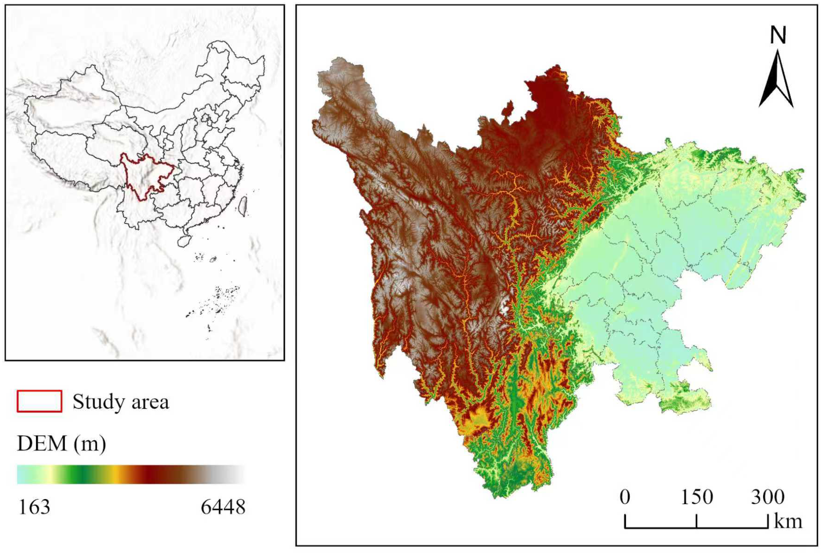
Sichuan Province is situated in the southwestern hinterland of China, with geographical coordinates ranging between 97°21′–108°33′ E and 26°03′–34°19′ N. It covers a total area of approximately 486,000 square kilometers, spanning roughly 1075 km from east to west and 921 km from north to south (Figure 1). The topography of Sichuan Province generally exhibits a stepped distribution pattern, higher in the west and lower in the east. The western region is predominantly highland and mountainous terrain, with elevations generally exceeding 4000 m. The central zone comprises the Hengduan Mountains and surrounding hilly and mountainous areas, where elevations typically range between 1000 and 3000 m. The eastern Sichuan Basin and Chengdu Plain feature relatively flat terrain, with elevations predominantly below 500 m. This substantial elevation gradient from plateau to plain results in pronounced spatial heterogeneity across Sichuan’s natural conditions and socioeconomic development.

Concurrently, from a socioeconomic perspective, regional economic development levels in Sichuan are highly coupled with topographical conditions [35]. The Chengdu Plain, leveraging its advantageous terrain, has evolved into a pivotal economic hub in Southwest China, boasting developed manufacturing and service sectors. Conversely, the western Sichuan plateau and mountainous regions face relatively lagging economic development, due to constraints such as scarce arable land, high costs of transport infrastructure construction, and poor industrial accessibility [36]. This topography-dominated development pattern has resulted in substantial disparities across Sichuan’s regions regarding infrastructure investment intensity and carbon emission levels.

As a vital ecological barrier in the upper Yangtze River basin and a strategic national hinterland, Sichuan is currently accelerating new urbanization and infrastructure development to address deficiencies, facing dual constraints of pursuing high-quality economic development while meeting the “dual carbon” goals [37]. Whether infrastructure investment, while stimulating the economy, has broken free from reliance on high-carbon pathways directly impacts the sustainability of regional green development [38]. Consequently, conducting spatiotemporal decoupling research on infrastructure investment and carbon emissions in Sichuan holds significant practical implications for addressing regional development imbalances and synergistically advancing ecological conservation and high-quality development along the Yangtze River Economic Belt.

2.2. Data Acquisition and Spatial Processing

2.2.1. Variable Definitions and Data Sources

This study employs two categories of variables: geospatial terrain indicators and socioeconomic panel data. The key variables are defined as follows:

(1) Fixed-asset investment (INV): Defined as the total investment in fixed assets at the prefecture-city level, measured in 100 million Chinese Yuan (CNY). The data are reported in nominal terms as published by the National Bureau of Statistics. To account for inflation effects, all monetary values were deflated to constant 2000 prices using the provincial fixed-asset investment price index obtained from the Sichuan Statistical Yearbook. In the Tapio decoupling model, the percentage change formulation ($\%\Delta$) inherently mitigates level effects of nominal scaling; nevertheless, the use of real values ensures consistency across the 21-year study period.

(2) Carbon dioxide emissions (CO₂): Total CO₂ emissions at the prefecture-city level, measured in 10⁴ tons (10,000 metric tons), sourced from the Emissions Database for Global Atmospheric Research (EDGAR v2024_GHG). EDGAR provides gridded emission estimates; city-level totals were extracted by matching the administrative city codes in the dataset. The data cover 2000–2021 for all 21 prefecture-level cities in Sichuan Province.

(3) Gross Domestic Product (GDP): Prefecture-city level GDP in 100 million CNY, deflated to constant 2000 prices using the provincial GDP deflator. GDP serves as a control variable in the Geodetector analysis.

(4) Per capita GDP (PGDP): GDP divided by year-end resident population (CNY/person, constant 2000 prices), reflecting the regional economic development level.

(5) Secondary Industry share (IS): The proportion of secondary industry value-added in GDP (%), indicating the industrial structure.

(6) Energy Intensity (EI): Energy consumption per unit of GDP (tons of standard coal equivalent per 10,000 CNY), reflecting the energy efficiency.

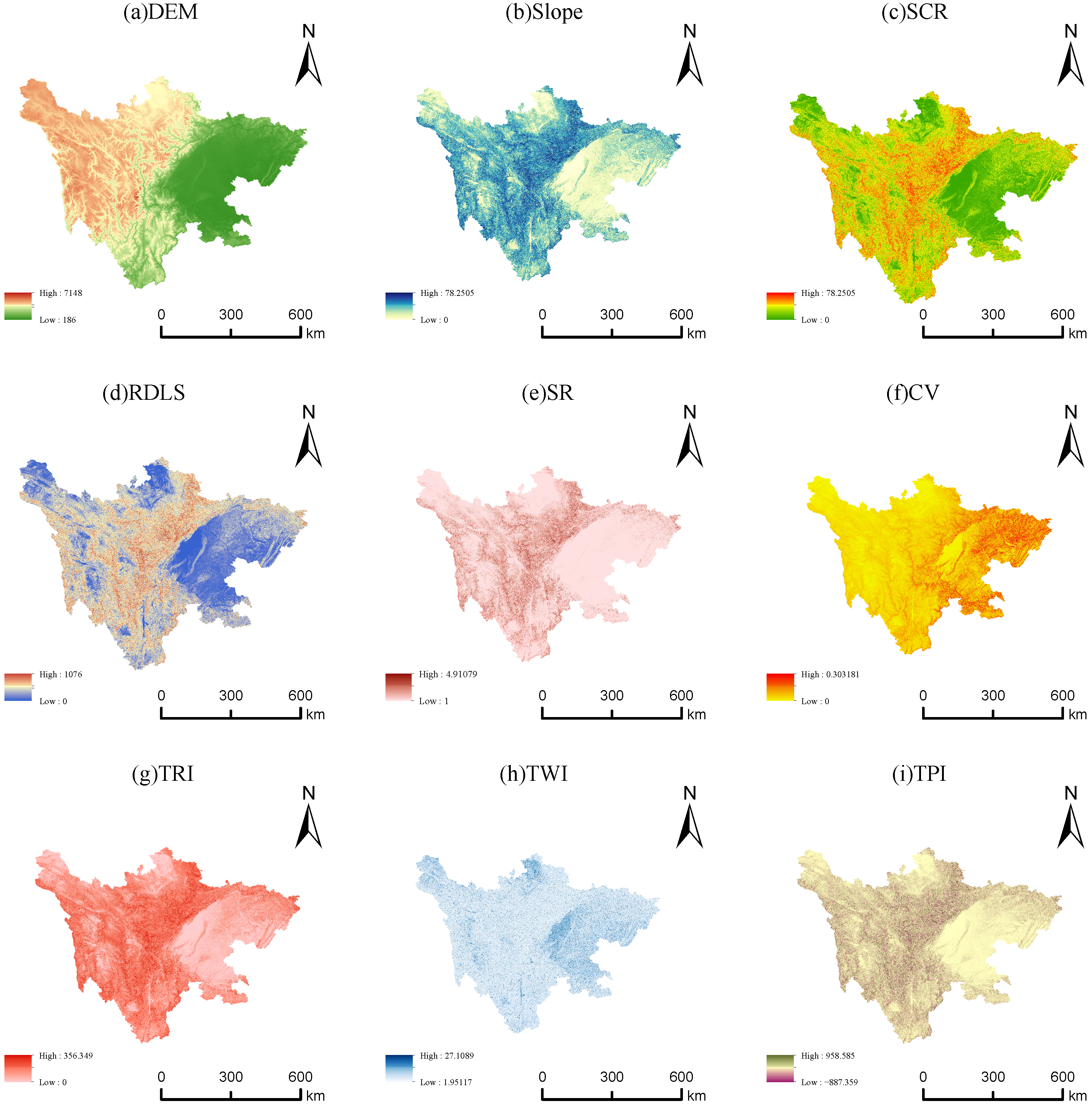
(7) Geospatial terrain indicators: Nine terrain metrics were initially derived from the Digital Elevation Model (DEM): DEM (elevation in meters), Slope (degrees), Slope Change Rate (SCR), Relief Degree of Land Surface (RDLS), Surface Roughness (SR), Coefficient of Variation of elevation (CV, dimensionless), Terrain Ruggedness Index (TRI), Terrain Wetness Index (TWI), and Terrain Position Index (TPI). Each indicator was computed as the city-level spatial average by performing zonal statistics over administrative boundaries.

DEM data (ASTER GDEM v3, 30 m resolution) were obtained from the Geospatial Data Cloud (https://www.gscloud.cn/). Derived terrain indicators were calculated using the Spatial Analyst module in ArcGIS 10.7: Slope was computed using the “Slope” tool; SCR was obtained as the second derivative of slope; RDLS, TRI, and TPI were derived using a 3 × 3 pixel moving window; TWI was calculated from hydrological analysis after depression filling; SR and CV were computed from neighborhood statistics.

GDP and fixed-asset investment data were sourced from the National Bureau of Statistics of China (https://data.stats.gov.cn/). The PGDP, IS, and EI were obtained from the Statistical Yearbooks of Sichuan Province (2001–2022 editions). The complete data sources and temporal coverage are summarized in

Table 1. Data sources and temporal coverage used in this study.

Variable	Unit	Source	Period
DEM	m	Geospatial Data Cloud 1	2020
Terrain indicators	various	Derived from DEM	2020
Fixed-asset investment	108 CNY	NBS 2	2000–2021
GDP	108 CNY	NBS 2	2000–2021
CO2 emissions	104 tons	EDGAR v2024_GHG 3	2000–2021
PGDP	CNY/person	Sichuan Yearbook 4	2000–2021
IS	%	Sichuan Yearbook 4	2000–2021
EI	tce/104 CNY	Sichuan Yearbook 4	2000–2021

¹ https://www.gscloud.cn/ (accessed on 26 December 2025); ² National Bureau of Statistics, https://data.stats.gov.cn/ (accessed on 26 December 2025); ³ https://edgar.jrc.ec.europa.eu/ (accessed on 27 December 2025); ⁴ https://tjj.sc.gov.cn/ (accessed on 27 December 2025).

.

2.2.2. Temporal Invariance of Terrain Variables

The TCI is constructed from a single-epoch DEM (2020), while the socioeconomic panel spans 2000–2021. This treatment is justified on the grounds that macro-scale topographic features—elevation, terrain position, and elevation variability—are geomorphologically stable over decadal timescales; anthropogenic landform changes (e.g., cut-and-fill for road construction) are negligible relative to the 30 m DEM resolution and city-wide spatial averaging. Consequently, the TCI is treated as a time-invariant city-specific characteristic, and the empirical identification of terrain effects on decoupling performance is fundamentally cross-sectional in nature. This design is analogous to studies that use fixed geographic endowments (e.g., ruggedness indices) as instruments or grouping variables in panel settings. We acknowledge that this cross-sectional identification precludes within-city causal inference; the group comparison and Geodetector analyses should therefore be interpreted as documenting systematic associations rather than establishing causality.

2.2.3. Descriptive Statistics

Table 2. Descriptive statistics of key variables.

Variable	N	Mean	Std. Dev.	Min	Max
Time-varying socioeconomic variables (city–year, 2000–2021)
INV (108 CNY)	462	830.5	1476.0	13.0	13,756.2
CO2 (104 tons)	462	1010.8	936.9	112.4	4190.2
GDP (108 CNY)	462	2170.0	6907.5	24.7	19,917.0
PGDP (CNY/person)	462	24,028.3	19,421.2	2438.0	103,386.0
IS (%)	462	43.8	12.7	4.5	102.1
EI (tons/104 CNY)	462	0.11	0.17	0.00	1.29
Urbanization rate	462	0.40	0.13	0.12	0.80
Time-invariant terrain variables (city-level)
TCI	21	0.338	0.124	0.151	0.591
DEM (m)	21	1189.7	1092.1	362.3	4186.7
CV	21	0.0215	0.0077	0.0077	0.0344
TPI	21	0.403	0.557	−0.341	1.616

Note: INV = fixed-asset investment; IS = secondary industry share; EI = energy intensity; PGDP = per capita GDP; TCI = Terrain Constraint Index; DEM = Digital Elevation Model; CV = Coefficient of Variation; TPI = Terrain Position Index. CO₂ data are from EDGAR v2024_GHG. Terrain variables are city-level zonal means derived from 2020 DEM.

presents summary statistics for the key variables across the 21 prefecture-level cities. The socioeconomic panel covers 2000–2021, yielding N = 462 city–year observations (21 cities × 22 years); N = 21 for time-invariant terrain variables.

Figure 2 illustrates the terrain and topographic characteristics of Sichuan Province, clearly showing the significant elevation gradient from the western plateau to the eastern basin.

2.3. Carbon Emission Decoupling Model

2.3.1. Model Specification

To rigorously quantify the dynamic nexus between regional economic development and carbon emissions, this study employs the Tapio decoupling elasticity model. Compared to the traditional Organisation for Economic Co-operation and Development (OECD) decoupling coefficient, the Tapio model introduces the concept of elasticity, effectively overcoming the sensitivity of this indicator to base period selection and providing a more refined classification of decoupling states [39,40]. The decoupling elasticity index is calculated as follows:

$$e={\displaystyle \frac{\Delta C/C}{\Delta G/G}}={\displaystyle \frac{\%\Delta C}{\%\Delta G}},$$

(1)

where e is the decoupling elasticity coefficient, C represents carbon emissions in the base period, G represents fixed-asset investment (INV, in constant 2000 prices) in the base period, $\Delta C=C_t-C_{t-1}$ represents the change in carbon emissions between the current period and the base period, and $\Delta G=G_t-G_{t-1}$ represents the change in fixed-asset investment between the current period and the base period. Note that G denotes investment rather than GDP throughout this study, as the focus is on the decoupling between infrastructure investment and carbon emissions.

2.3.2. Classification of Decoupling States

Based on the positive or negative signs of $\Delta C$ and $\Delta G$, as well as the value of the elasticity coefficient e, the Tapio model categorizes the coordination between economic growth and environmental impact into eight logical types (

Table 3. Decoupling state classification criteria based on the Tapio model.

Decoupling State	$\mathbf{\Delta }\mathit{G}$	$\mathbf{\Delta }\mathit{C}$	e	Interpretation
SD	>0	<0	<0	Ideal state
WD	>0	>0	$0<e<0.8$	Good progress
RD	<0	<0	$e>1.2$	Economic decline
EC	>0	>0	$0.8\le e\le 1.2$	Synchronized growth
RC	<0	<0	$0.8\le e\le 1.2$	Synchronized decline
END	>0	>0	$e>1.2$	Unsustainable
SND	<0	>0	<0	Worst state
WND	<0	<0	$0<e<0.8$	Slight improvement

). Specifically, the model utilizes 0.8 and 1.2 as the critical threshold values for defining these decoupling states (see Appendix A for a numerical example).

(1) Decoupling States ($\mathit{e}<\mathbf{0.8}$): These include Strong Decoupling (SD), Weak Decoupling (WD), and Recessionary Decoupling (RD). Among these, SD is the ideal state for low-carbon development, characterized by an absolute decline in carbon emissions while the economy continues to grow.

(2) Coupling States ($\mathbf{0.8}\le \mathit{e}\le \mathbf{1.2}$): These include Expansive Coupling (EC) and Recessionary Coupling (RC), indicating that the growth rates of carbon emissions and the economy are largely synchronized.

(3) Negative Decoupling States ($\mathit{e}>\mathbf{1.2}$ or specific conditions): These include Expansive Negative Decoupling (END), Strong Negative Decoupling (SND), and Weak Negative Decoupling (WND). Among these, SND is the most unsustainable state, characterized by increasing carbon emissions despite economic recession.

2.4. Construction of Terrain Constraint Index (TCI)

2.4.1. Indicator Selection

Terrain features primarily influence the spatial distribution of carbon emissions by restricting the population concentration, increasing the infrastructure construction costs, and reducing the available buildable land [41]. Although nine terrain indicators were initially calculated (as shown in Figure 2), this study ultimately selected three fundamental indicators for constructing the TCI based on correlation analysis and multicollinearity testing.

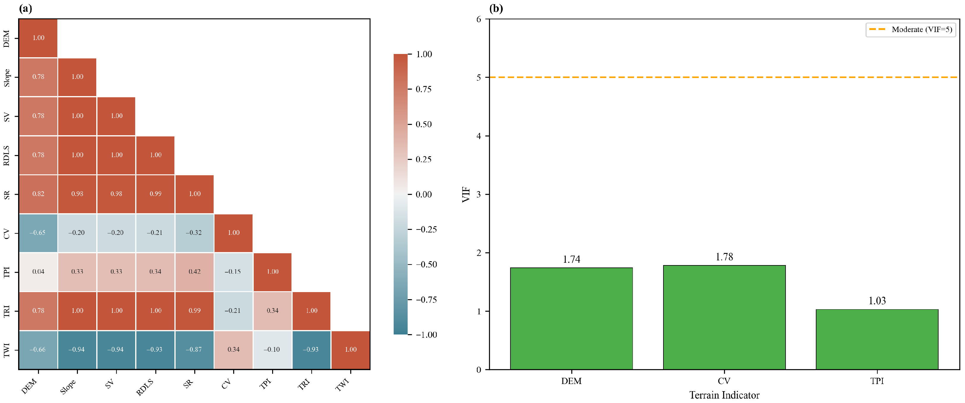
Selection Process: First, Pearson correlation analysis was conducted among all terrain indicators. Indicators with high correlation coefficients ($r>0.85$) were identified as potentially redundant. Second, Variance Inflation Factor (VIF) analysis was performed to detect multicollinearity. The results of the correlation and VIF analysis for all nine terrain indicators are presented in

Table 4. Correlation coefficients and VIF values for all terrain indicators.

Indicator	DEM	Slope	SCR	RDLS	SR	CV	TPI	TRI	VIF
DEM	1.00								47.2
Slope	0.78	1.00							>105
SCR	0.78	1.00	1.00						>105
RDLS	0.78	1.00	1.00	1.00					>105
SR	0.82	0.98	0.98	0.99	1.00				1428.9
CV	−0.65	−0.20	−0.20	−0.21	−0.32	1.00			14.9
TPI	0.04	0.33	0.33	0.34	0.42	−0.15	1.00		1.1
TRI	0.78	1.00	1.00	1.00	0.99	−0.21	0.34	1.00	>105
TWI	−0.66	−0.94	−0.94	−0.93	−0.87	−0.05	−0.10	−0.93	98.9

Note: VIF values > 10 indicate severe multicollinearity.

. The analysis reveals severe multicollinearity among several indicators: Slope, SCR, RDLS, SR, and TRI all exhibit extremely high VIF values (ranging from 98.9 to over 100,000), indicating strong redundancy. In contrast, the DEM (VIF = 47.2), CV (VIF = 14.9), and TPI (VIF = 1.1) show relatively lower multicollinearity levels.

Based on the correlation and VIF analysis results, the final indicator combination was selected to ensure the VIF values remain below 5, indicating acceptable multicollinearity levels. As shown in Figure 3, the selected three indicators (DEM, CV, and TPI) demonstrate low inter-correlation and acceptable VIF values (maximum VIF = 1.78).

Final Selected Indicators: Based on the above criteria, three indicators were selected with a maximum VIF of 1.78:

(1) DEM: Represents the vertical gradient of terrain. Higher elevations typically correspond to lower temperatures and thinner oxygen levels, forming natural barriers to industrial production and human settlement. Elevation directly affects construction material transportation costs and equipment operation efficiency.

(2) CV: Calculated as the ratio of the elevation standard deviation to mean elevation, it measures internal terrain dispersion and unevenness. A higher CV indicates more pronounced topographic variation within the area, making it difficult to form contiguous construction land and requiring more complex engineering solutions.

(3) TPI: Indicates the relative position within the landscape (ridge vs. valley). TPI reflects the local topographic context and influences drainage patterns, accessibility, and construction site selection.

Excluded Indicators and Rationale: Six indicators were excluded from the final TCI construction due to high multicollinearity: (1) Slope was highly correlated with RDLS ($r=0.94$); (2) SCR showed redundancy with slope; (3) RDLS was correlated with multiple indicators; (4) SR was highly correlated with TRI ($r=0.91$); (5) TRI showed high correlation with slope-related indicators; (6) TWI primarily reflects hydrological accumulation potential rather than direct construction constraints.

2.4.2. Game Theory-Based Combination Weighting Method

To eliminate dimensional differences among indicators and balance subjective and objective weighting approaches, this study employs a game theory-based combination weighting method that integrates the entropy weight method and the CRITIC method.

Step 1: Entropy Weight Method. The entropy weight method determines weights based on the information content of each indicator. Indicators with larger variation carry more information and receive higher weights:

$$w_j^E={\displaystyle \frac{1-e_j}{{\sum }_{j=1}^n(1-e_j)}},$$

(2)

where $e_j$ is the entropy value of indicator j.

Step 2: CRITIC Method. The CRITIC method considers both the contrast intensity (standard deviation) and conflict (correlation) between indicators:

$$w_j^C={\displaystyle \frac{C_j}{{\sum }_{j=1}^n{C}_j}},C_j={\sigma }_j\sum _{k=1}^n(1-r_{jk}),$$

(3)

where ${\sigma }_j$ is the standard deviation of indicator j, and $r_{jk}$ is the correlation coefficient between indicators j and k.

Step 3: Game Theory Combination. The final combined weights are obtained by optimizing the linear combination of the two weight sets to minimize deviation:

$$w_j=\alpha ·w_j^E+(1-\alpha )·w_j^C,$$

(4)

where $\alpha$ is determined by minimizing the sum of squared deviations from both original weight sets.

The calculation results are presented in

Table 5. Calculation results of weights for terrain factors using game theory combination method.

Indicator	Entropy Weight	CRITIC Weight	Combined Weight (%)
DEM	0.605	0.347	47.6
CV	0.156	0.374	26.5
TPI	0.239	0.279	25.9

. DEM carries the highest combined weight (47.6%), followed by CV (26.5%) and TPI (25.9%).

2.4.3. TCI Calculation and Classification

Based on the determined weights, the TCI for each region is calculated using the weighted sum method:

$$TC{I}_i=\sum _{j=1}^3{w}_j\times x_{ij}^{\prime }.$$

(5)

The TCI values are then classified into five levels using natural breaks: Very Low (0–0.2), Low (0.2–0.3), Medium (0.3–0.4), High (0.4–0.5), and Very High (0.5–1.0). The higher the index, the more challenging the terrain conditions in the area, indicating higher natural costs and difficulties in land development.

2.5. Statistical Analysis Methods

2.5.1. Group Comparison Analysis

To examine the correlation between terrain complexity and decoupling performance, this study employs group comparison analysis based on the TCI classification levels. This approach is particularly suitable when the association may be nonlinear and when sample sizes within groups are relatively small.

Descriptive Statistics: For each TCI level group, we calculate the mean, standard deviation, and median of the decoupling elasticity, as well as the proportion of different decoupling states.

Good Decoupling Ratio: We define “good decoupling” as the combination of SD and WD states, representing favorable carbon emission performance. The good decoupling ratio for each TCI level is calculated as

$$GD{R}_h={\displaystyle \frac{N_{SD,h}+N_{WD,h}}{N_h}}\times 100\%,$$

(6)

where $N_{SD,h}$ and $N_{WD,h}$ are the number of observations in the SD and WD states within TCI level h, and $N_h$ is the total number of observations in that level.

Kruskal–Wallis H Test: To test whether significant differences exist among TCI groups, we employ the Kruskal–Wallis H test, a non-parametric alternative to one-way ANOVA:

$$H={\displaystyle \frac{12}{N(N+1)}}\sum _{h=1}^k{\displaystyle \frac{R_h^2}{n_h}}-3(N+1),$$

(7)

where $R_h$ is the sum of ranks in group h, $n_h$ is the sample size of group h, and N is the total sample size.

Mann–Whitney U Test: For pairwise comparisons between TCI groups, we use the Mann–Whitney U test to identify which specific group pairs show significant differences.

2.5.2. Geographical Detector

The Geographical Detector, originally proposed by Wang et al. [42], is a statistical method that detects spatial heterogeneity and reveals its driving factors without assuming linear associations [43,44,45]. It effectively identifies the explanatory power of influencing factors and their interactions on the spatial distribution of the dependent variable [46]. This study employs the model to address two primary objectives.

First is to quantify the independent contributions of topographic constraints (TCI) and various control variables to the spatial patterns of carbon decoupling. Second is to investigate whether natural topography reinforces the spatial effects of carbon lock-in through interactions with socioeconomic factors.

The specific operational steps are as follows:

(1) Discretization. Continuous variables were discretized into categorical grades using quantile-based classification, which ensures approximately equal sample sizes across strata. Given the small sample size (N = 21 cities), all variables were discretized into k = 3 classes to ensure a minimum of 5 observations per stratum, following the recommendation that each stratum should contain sufficient observations for reliable variance estimation. The choice of k = 3 was further validated through sensitivity analysis: we repeated the factor detection with k = 4 and k = 5 classes and found that Investment consistently ranked first across all specifications (q = 0.401, 0.469, and 0.639 for k = 3, 4, 5, respectively). Individual q-values for other factors showed higher variability across specifications (e.g., TCI: q = 0.100 at k = 3 vs. 0.485 at k = 5), reflecting the sensitivity inherent to small-sample discretization. We report the k = 3 results as the primary specification, due to the more balanced stratum sizes and conservative estimates.

(2) The q statistic is used to measure the explanatory power of each factor X on the spatial differentiation of the dependent variable Y, as expressed by the following formula:

$$q=1-{\displaystyle \frac{{\sum }_{h=1}^L{N}_h{\sigma }_h^2}{N{\sigma }^2}},$$

(8)

where $h=1,2,\dots ,L$ represents the strata of variable X; $N_h$ and N are the number of units in stratum h and the whole region, respectively; and ${\sigma }_h^2$ and ${\sigma }^2$ are the variance of Y in stratum h and the whole region, respectively.

(3) Interaction detection examines whether two factors together have enhanced or weakened explanatory power compared to their individual effects. The interaction types include nonlinear enhancement (q(X1∩X2) > q(X1) + q(X2)), bi-factor enhancement (max(q(X1), q(X2)) < q(X1∩X2) < q(X1) + q(X2)), and weakening effects.

2.6. Research Framework

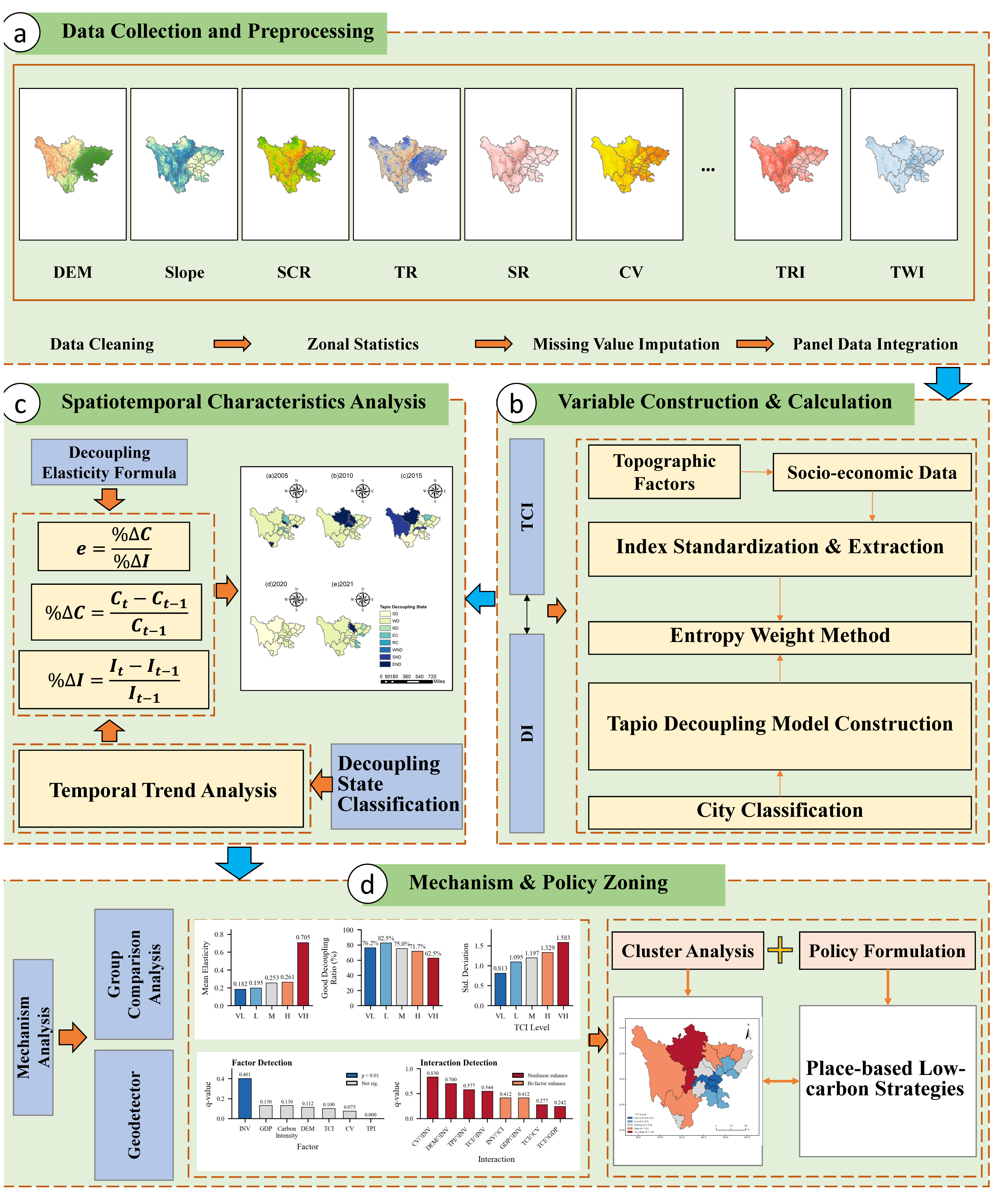
This study follows a systematic technical roadmap to investigate the spatiotemporal decoupling linkage between infrastructure investment and carbon emissions in complex terrain regions (Figure 4). The research framework consists of four main stages:

Stage 1: Data Acquisition and Processing. Multi-source data including DEM, socioeconomic indicators, and carbon emission data were collected and preprocessed. Terrain-derived indicators were calculated using ArcGIS spatial analysis tools.

Stage 2: TCI Construction. Three terrain indicators (DEM, CV, TPI) were selected and weighted using game theory combination method to calculate TCI. Cities were classified into five terrain constraint levels.

Stage 3: Decoupling Analysis. The Tapio decoupling model was employed to calculate decoupling elasticity coefficients between infrastructure investment and carbon emissions. Spatiotemporal evolution patterns were analyzed.

Stage 4: Statistical Analysis. Group comparison analysis examined the correlation between terrain complexity and decoupling performance. Geodetector quantified the explanatory power of terrain constraints and interaction effects.

3. Results

3.1. Spatial Characteristics of Terrain Constraint Index

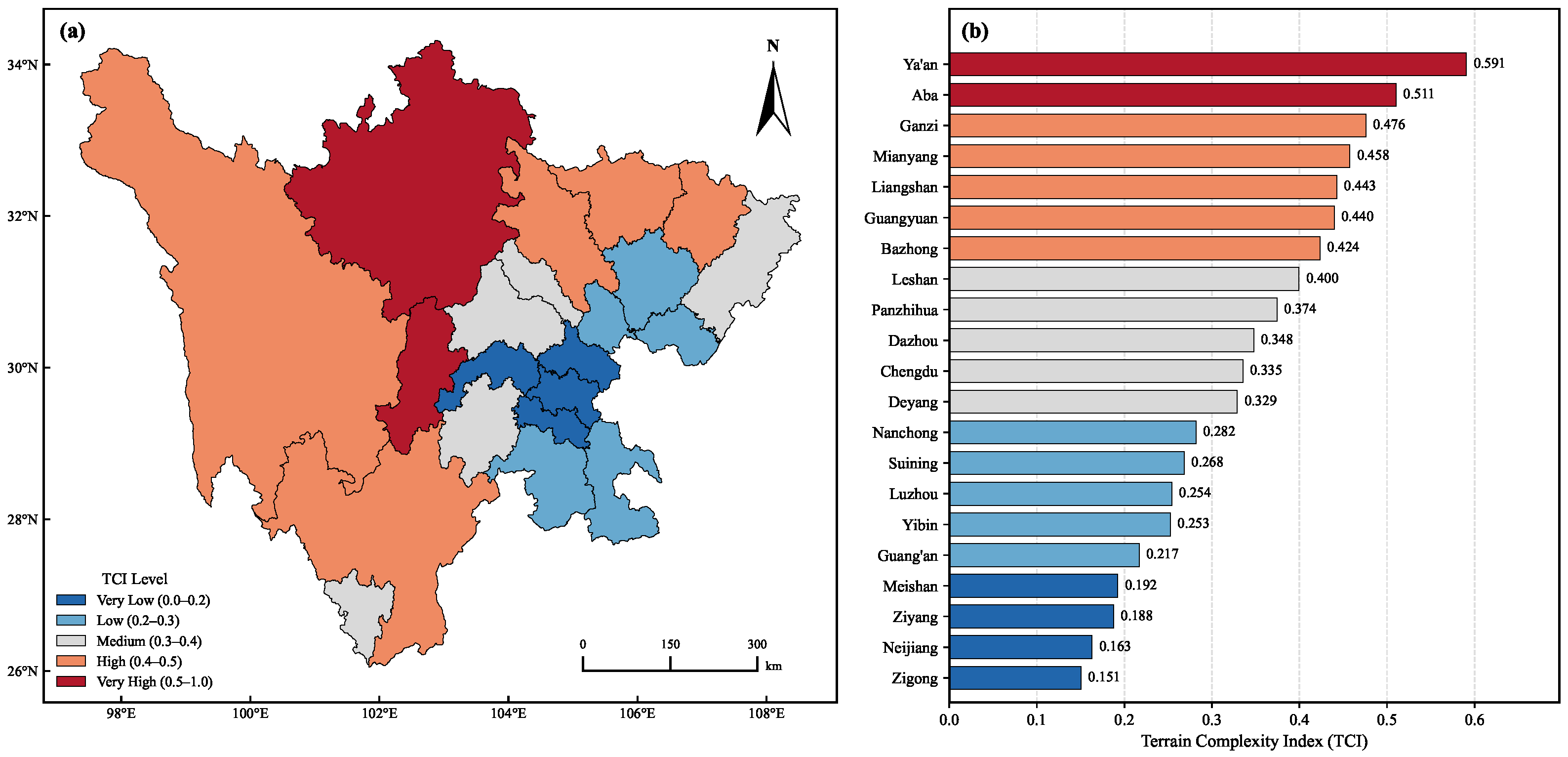
This study categorizes cities and prefectures in Sichuan Province into five terrain complexity levels based on the TCI calculated using the game theory combination weighting method (

Table 6. The calculation results and classification of TCI for cities in Sichuan Province.

TCI Level	Cities	TCI Range
Very High (0.5–1.0)	Ya’an, Aba	0.511–0.591
High (0.4–0.5)	Ganzi, Mianyang, Liangshan, Guangyuan, Bazhong	0.424–0.476
Medium (0.3–0.4)	Leshan, Panzhihua, Dazhou, Chengdu, Deyang	0.329–0.400
Low (0.2–0.3)	Nanchong, Suining, Yibin, Luzhou	0.252–0.282
Very Low (0–0.2)	Guang’an, Meishan, Ziyang, Neijiang, Zigong	0.151–0.217

). Across the entire province of Sichuan, the TCI exhibits highly significant spatial heterogeneity, presenting an overall pattern of “high in the west, low in the east, with a stepped distribution”. The TCI values range from 0.151 (Zigong) to 0.591 (Ya’an), demonstrating substantial variation in terrain constraints across the region (Figure 5).

Very High TCI Regions (TCI > 0.5) include Ya’an (0.591) and Aba (0.511), representing the most topographically complex areas in Sichuan Province. These regions are characterized by extremely high elevations, dramatic terrain variation, and significant engineering challenges for infrastructure development.

High TCI Regions (0.4–0.5) include Ganzi, Mianyang, Liangshan, Guangyuan, and Bazhong. These areas are primarily located in the western plateau and northern mountainous zones, facing substantial terrain constraints that increase infrastructure construction costs.

Medium TCI Regions (0.3–0.4) include Leshan, Panzhihua, Dazhou, Chengdu, and Deyang. These transitional zones connect the mountainous west with the basin east, presenting moderate topographical challenges.

Low TCI Regions (0.2–0.3) include Nanchong, Suining, Yibin, and Luzhou. These hilly areas offer relatively favorable conditions for infrastructure development compared to mountainous regions.

Very Low TCI Regions (TCI < 0.2) include Guang’an, Meishan, Ziyang, Neijiang, and Zigong. Located within the Sichuan Basin, these areas enjoy the most favorable terrain conditions, enabling efficient infrastructure construction with lower carbon intensity.

In summary, this spatial gradient of topographical constraints in Sichuan largely determines the carbon efficiency baseline for fixed-asset investments across regions, creating a stark contrast between the “low-constraint, high-efficiency” eastern areas and the “high-constraint, low-efficiency” western areas.

3.2. Spatiotemporal Evolution of Carbon Emissions and Decoupling Status

3.2.1. Spatiotemporal Evolution Characteristics of Carbon Emissions

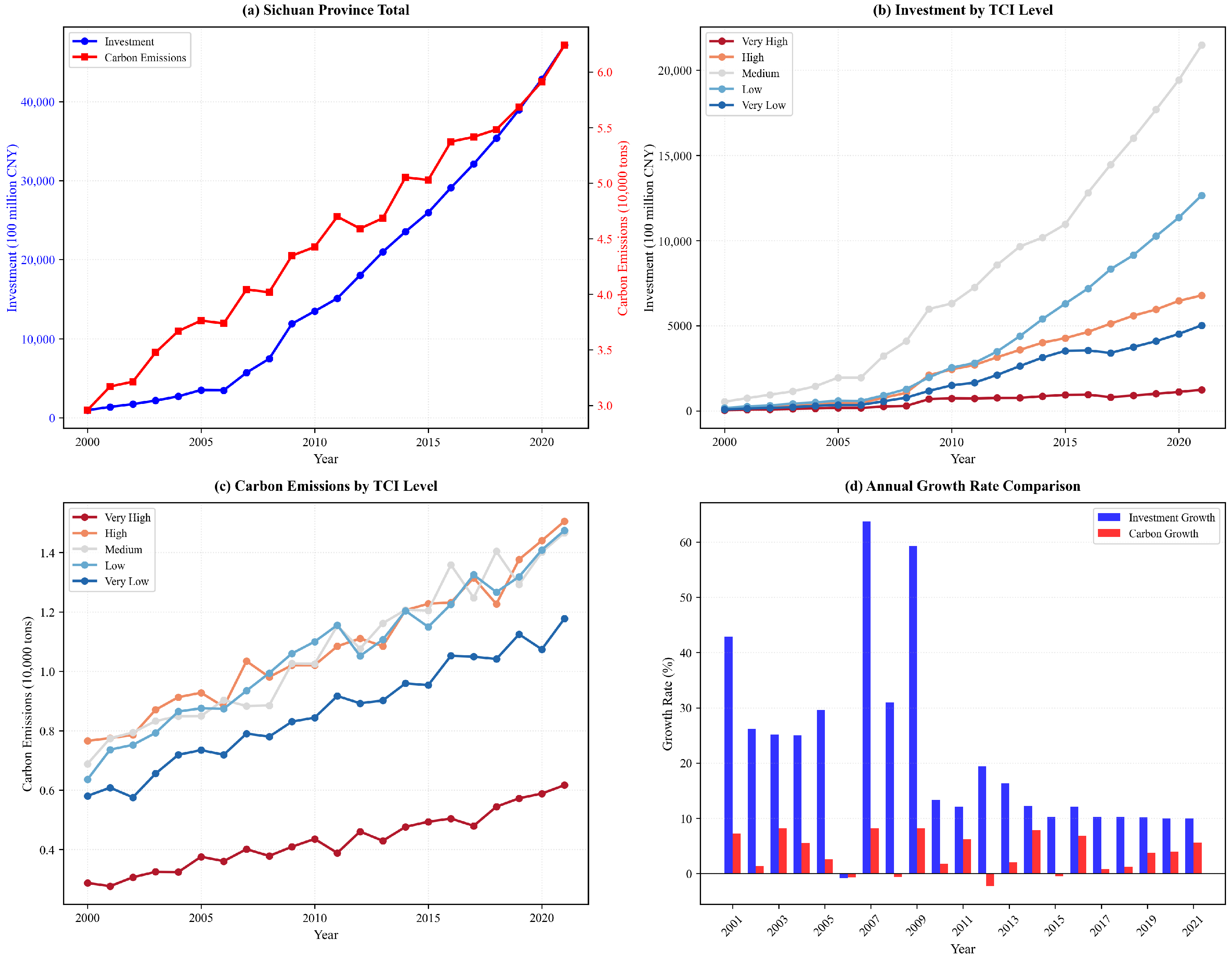
Sichuan Province’s carbon emissions trajectory exhibits path-dependent expansion characteristics closely coupled with the fixed-asset investment cycle. At the macro level (Figure 6a), provincial emissions reached a peak growth momentum around 2013, subsequently entering a plateau phase marked by high-frequency fluctuations. Significant hierarchical differentiation emerges when classified by TCI (Figure 6c): Very Low and Low TCI regions dominate total emissions but exhibit stabilizing growth rates, while High and Very High TCI regions demonstrate higher volatility, with carbon output showing high synchrony with investment surges (Figure 6b).

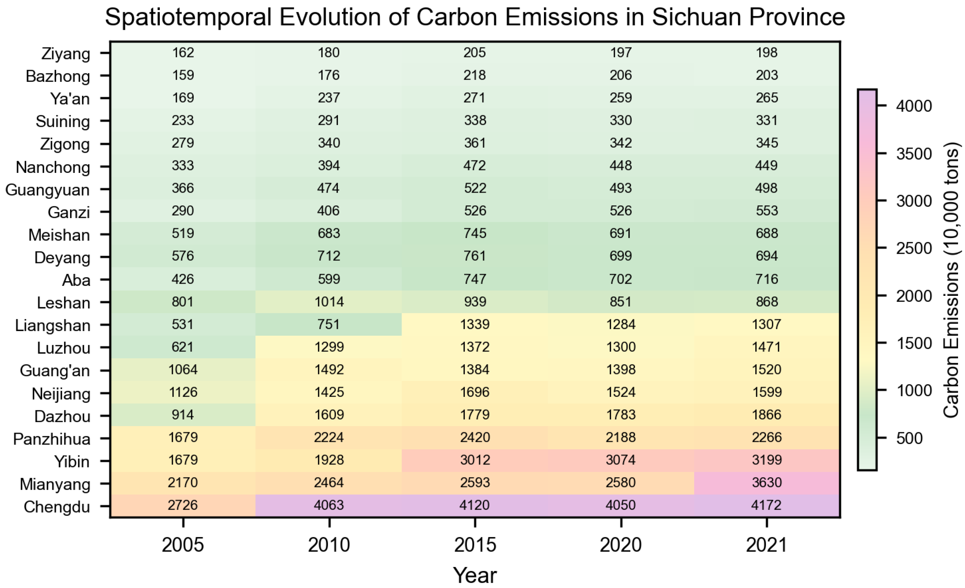
At the municipal level, spatial heatmaps (Figure 7) clearly delineate Chengdu’s status as an enduring core of emissions, primarily driven by lock-in effects from its high-density industry and urbanization. Concurrently, industrial corridor cities like Yibin and Mianyang have emerged as secondary growth poles with rapidly intensifying heat values, contrasting sharply with peripheral cities like Bazhong and Ganzi that remain in a state of low emissions and high terrain constraints. This pattern suggests that Very Low and Low TCI regions may determine the baseline for provincial emissions, while High and Very High TCI regions potentially serve as key incremental areas for emission fluctuations. This could be attributed to the fact that high TCI areas typically have lower baseline emissions due to limited industrial activity but experience significant emission spikes during infrastructure construction phases when high-carbon activities such as tunnel excavation, bridge construction, and material transportation are concentrated within short periods.

3.2.2. Analysis of Decoupling Status Between Investment and Carbon Emissions

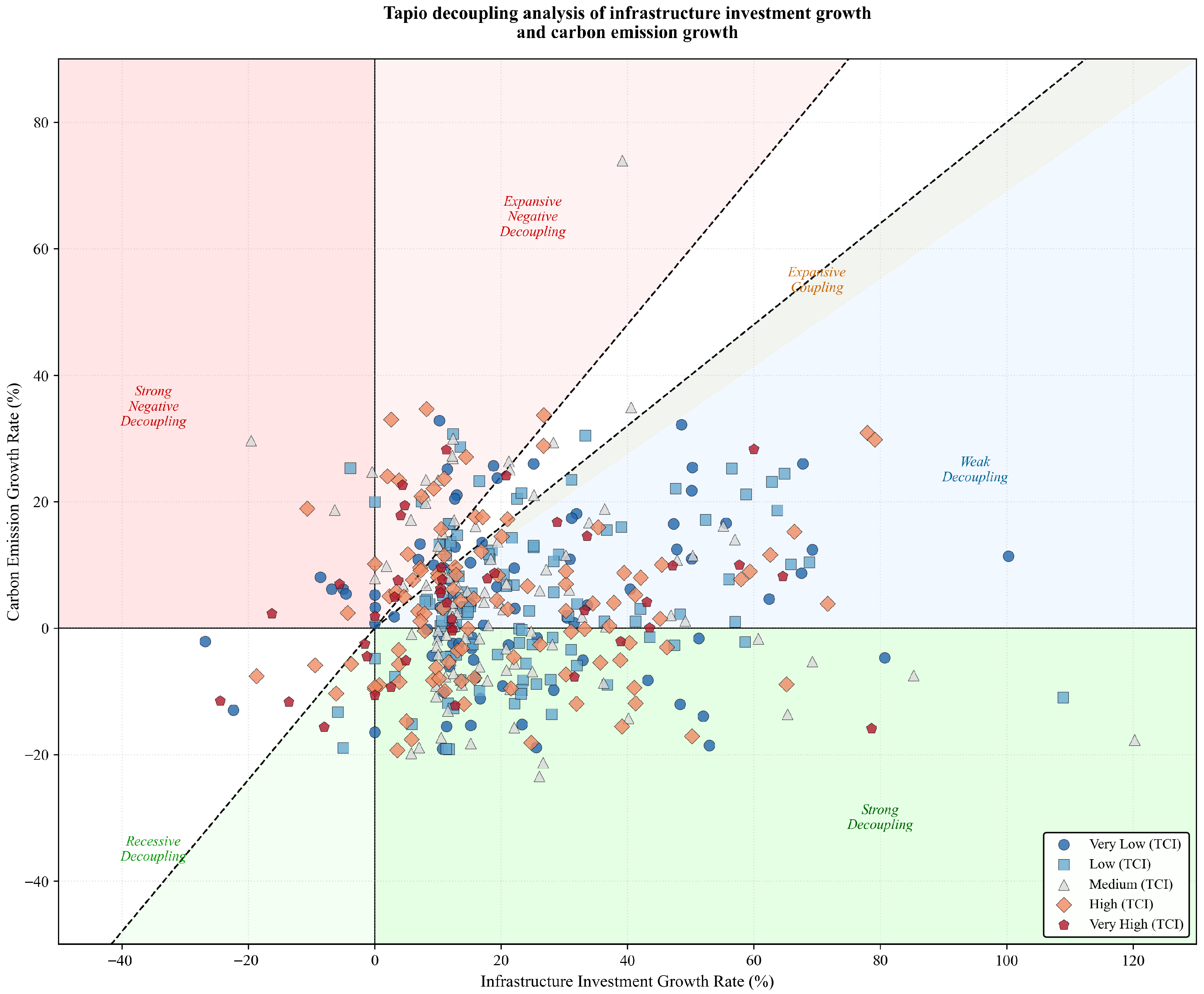
The decoupling linkage between investment and carbon emissions reveals a deep-seated “terrain–efficiency” penalty mechanism. The provincial sample primarily clusters within the WD and EC intervals, indicating that economic growth remains constrained by incremental carbon emissions. This evolution exhibits distinct TCI gradient characteristics: Very Low and Low TCI cities, benefiting from agglomeration economies and technological spillovers, are accelerating their migration toward the SD quadrant; whereas High and Very High TCI regions, scattered across the map (Figure 8), demonstrate higher dispersion and frequently fall into END during intensive infrastructure construction phases.

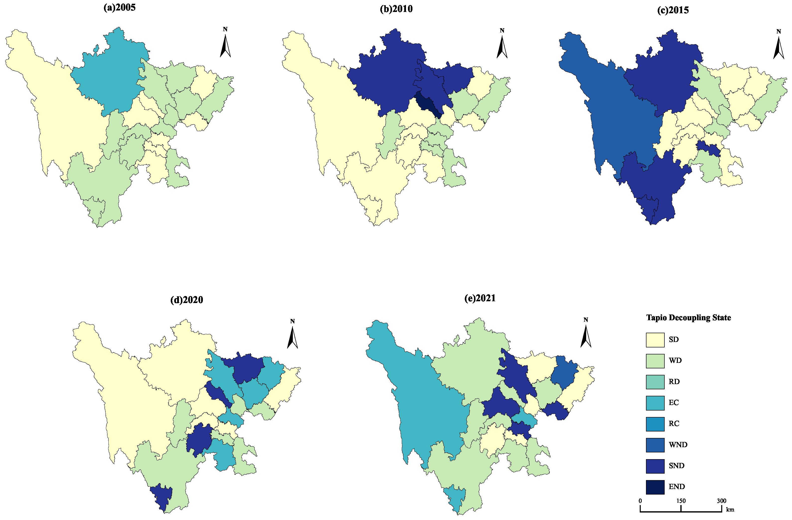
Spatiotemporal mapping (Figure 9) further highlights this divergence, revealing the province’s transition from historical coupling to fragmented decoupling. However, frequent decoupling setbacks in western and northeastern Sichuan (High and Very High TCI regions) highlight structural barriers: the high carbon intensity required to overcome geographical friction—such as tunnel construction and high-elevation logistics—largely offsets the marginal efficiency gains from new investments. Consequently, Sichuan’s achievement of stable “strong decoupling” remains spatially constrained by carbon costs inherent to traversing complex terrain.

3.3. Group Comparison Analysis of Terrain Constraints on Decoupling Performance

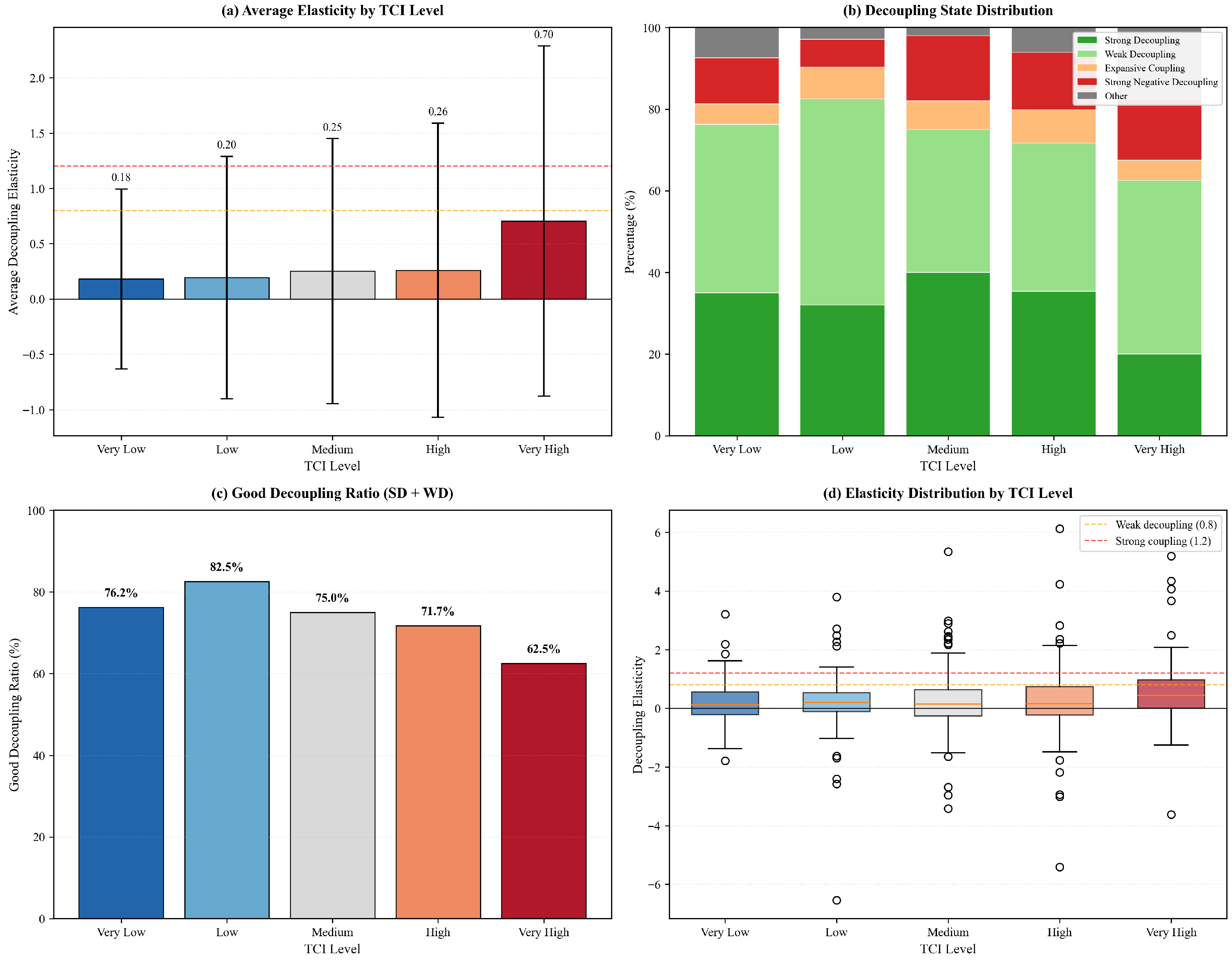
To examine the correlation between terrain complexity and decoupling performance, this study employs group comparison analysis based on the five TCI classification levels. The results reveal a clear negative correlation between terrain complexity and decoupling outcomes (

Table 7. Group comparison results: decoupling characteristics by TCI level.

TCI Level	N	Mean Elasticity	Std. Dev.	Good Decoupling Ratio (%)	Avg. TCI
Very Low	80	0.182	0.813	76.2	0.173
Low	103	0.195	1.095	82.5	0.255
Medium	100	0.253	1.197	75.0	0.357
High	99	0.261	1.329	71.7	0.448
Very High	40	0.705	1.583	62.5	0.551

Note: Good Decoupling Ratio = (Strong Decoupling + Weak Decoupling)/Total observations × 100%.

).

The group comparison results reveal several important findings:

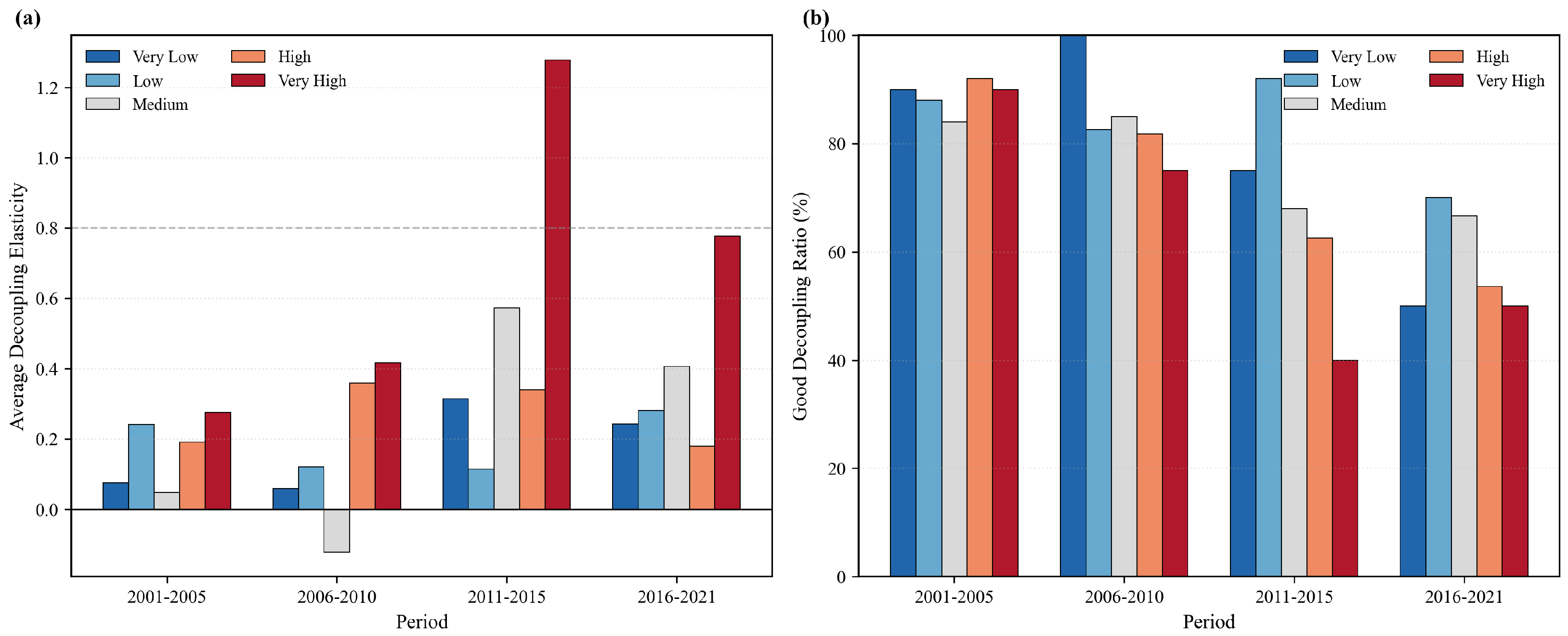
(1) The average decoupling elasticity increases with the terrain complexity. The mean elasticity rises from 0.182 in Very Low TCI regions to 0.705 in Very High TCI regions, representing a 287% increase. Lower elasticity values indicate better decoupling performance (carbon emissions growing slower than investment), confirming that regions with higher terrain complexity tend to face larger challenges in achieving carbon-efficient infrastructure development.

(2) The good decoupling ratio decreases with the terrain complexity. The proportion of observations achieving good decoupling (Strong Decoupling + Weak Decoupling) decreases from 82.5% in Low TCI regions to 62.5% in Very High TCI regions. Notably, the Low TCI group shows the highest good decoupling ratio, suggesting that moderate terrain conditions may be optimal for balancing development and carbon efficiency.

(3) The variability increases with the terrain complexity. The standard deviation of elasticity increases from 0.813 in Very Low TCI regions to 1.583 in Very High TCI regions, indicating that decoupling outcomes become more unpredictable in topographically complex areas.

Statistical Significance Tests

Table 8. Statistical test results for group differences.

Test	Statistic	Raw p	Adj. p	Interpretation
Overall Test
Kruskal–Wallis H	5.200	0.267	–	Not significant (${\epsilon }^2$ = 0.012)
Pairwise Comparisons (Mann–Whitney U, Bonferroni-adjusted, m = 10)
Very Low vs Very High	1216.0	0.033	0.328	Not significant after correction
Low vs Very High	1681.0	0.089	0.887	Not significant after correction
Medium vs Very High	1587.0	0.057	0.571	Not significant after correction
High vs Very High	1634.0	0.108	1.000	Not significant after correction

Note: Adj. p = raw p-value × 10 (Bonferroni correction for 10 pairwise comparisons), capped at 1.0. ${\epsilon }^2$ = epsilon-squared effect size.

presents the results of the statistical tests examining differences among TCI groups. The overall Kruskal–Wallis H test yields H = 5.200 (p = 0.267), with a negligible effect size (${\epsilon }^2$ = H/(N−1) = 5.200/421 = 0.012), indicating that the five TCI groups do not differ significantly in decoupling elasticity at conventional levels. This result warrants a cautious interpretation of the group differences.

Uncorrected pairwise Mann–Whitney U tests suggest that the Very Low vs. Very High TCI comparison yields the smallest raw p-value (U = 1216.0, p = 0.033); however, after Bonferroni correction for 10 pairwise comparisons, no pair remains statistically significant at the 0.05 level. This outcome is not unexpected given the modest sample sizes within groups (particularly Very High TCI with only two cities and 40 city-year observations) and the high within-group variability of decoupling elasticity. Rather than interpreting these results as evidence of statistically confirmed group differences, we characterize the pattern as a gradual monotonic trend: the average elasticity increases progressively from 0.182 (Very Low) to 0.705 (Very High), and the good decoupling ratio decreases from 82.5% to 62.5%. These descriptive patterns are consistent with the hypothesis that terrain complexity is associated with worse decoupling outcomes, but the statistical evidence remains suggestive rather than conclusive due to the limited statistical power.

Figure 10 presents the group comparison results across different TCI levels. The comparison reveals that the Very High TCI regions consistently show higher average elasticity, higher variability, and lower good decoupling ratios compared to lower TCI regions.

Figure 11 presents additional group comparison results across different TCI levels. The comparison reveals that the Very High TCI regions consistently show higher variability and more frequent negative decoupling episodes compared to lower TCI regions.

3.4. Driver Detection and Interaction Analysis of Spatial Differentiation

The Geodetector analysis reveals the explanatory power of different factors on the spatial differentiation of the good decoupling ratio across cities. The analysis uses city-level aggregated data (21 cities) with the good decoupling ratio as the dependent variable (

Table 9. Geodetector factor detection results.

Factor	q-Value	p-Value	Significance
Investment	0.401	0.010	***
GDP	0.130	0.287
Carbon Intensity	0.130	0.287
DEM	0.112	0.344
TCI	0.100	0.387
CV	0.075	0.498
TPI	0.000	1.000

Note: *** p < 0.01. Significance tested using F-test.

).

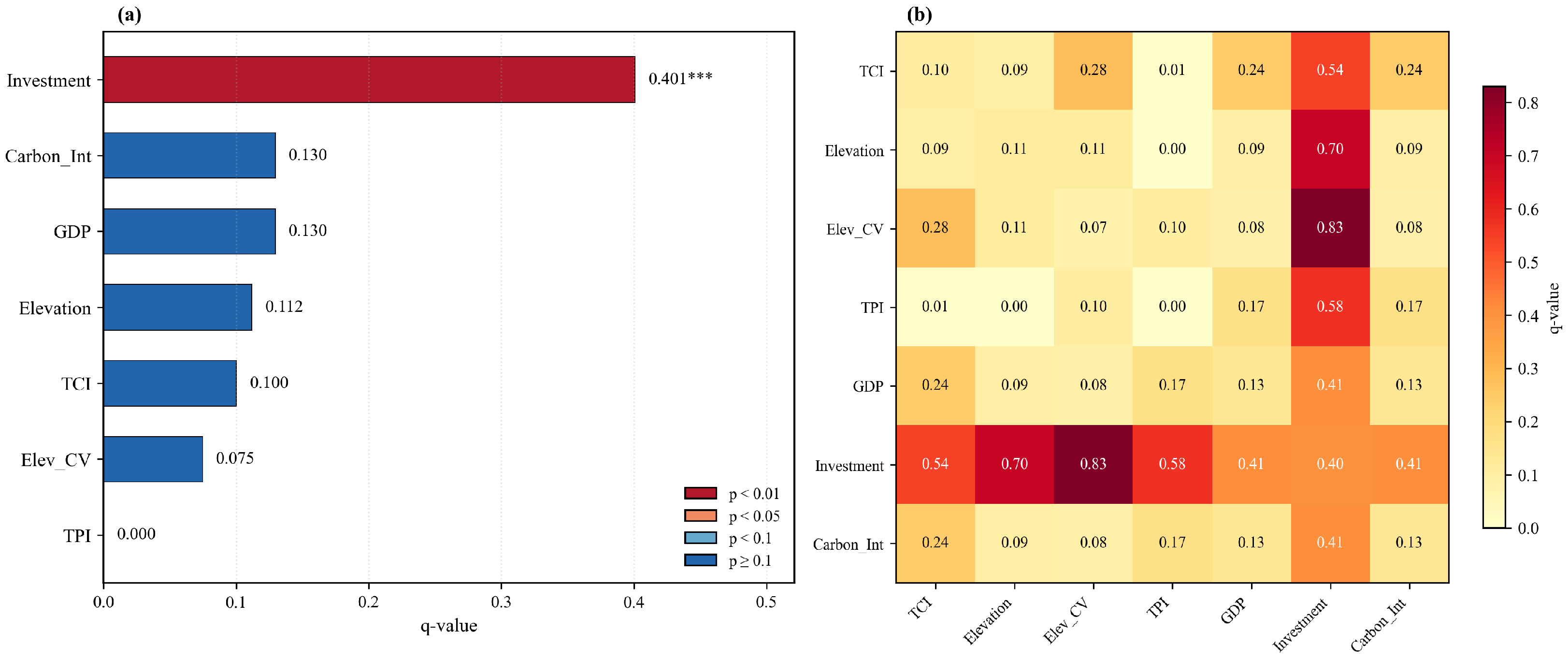
The factor detection results indicate that Investment has the highest explanatory power (q = 0.401, p = 0.010) for the spatial differentiation of good decoupling ratio, suggesting that the infrastructure investment scale is the primary factor associated with the decoupling performance differences among cities. The terrain-related factors (TCI, DEM, CV) show moderate q-values (0.075–0.112) but are not individually significant, suggesting that the terrain effects may operate through interaction with other factors rather than independently.

The interaction detection analysis reveals significant enhancement effects between terrain factors and socioeconomic factors (

Table 10. Geodetector interaction detection results.

Interaction	q(X1∩X2)	q(X1)	q(X2)	Type
CV ∩ Investment	0.830	0.075	0.401	Nonlinear enhance
DEM ∩ Investment	0.700	0.112	0.401	Nonlinear enhance
TPI ∩ Investment	0.577	0.000	0.401	Nonlinear enhance
TCI ∩ Investment	0.544	0.100	0.401	Nonlinear enhance
Investment ∩ Carbon Int.	0.412	0.401	0.130	Bi-enhance
GDP ∩ Investment	0.412	0.130	0.401	Bi-enhance
TCI ∩ CV	0.277	0.100	0.075	Nonlinear enhance
TCI ∩ GDP	0.242	0.100	0.130	Nonlinear enhance

Note: Nonlinear enhance: q(X1∩X2) > q(X1) + q(X2); Bi-enhance: max(q(X1), q(X2)) < q(X1∩X2) < q(X1) + q(X2).

). All interactions involving Investment show substantial increases in explanatory power.

The interaction results reveal several important findings:

(1) Terrain–Investment interactions show strong nonlinear enhancement. The interaction between CV and Investment produces the highest q-value (0.830), far exceeding the sum of individual effects (0.476). Similarly, DEM ∩ Investment (q = 0.700) and TCI ∩ Investment (q = 0.544) show substantial enhancement. These results are consistent with the hypothesis that the terrain complexity amplifies the carbon emission effects of infrastructure investment.

(2) The mechanism of terrain effects. The strong interaction effects suggest that terrain constraints are associated with decoupling performance primarily through modifying the efficiency of infrastructure investment rather than through direct independent effects. In regions with high terrain complexity, each unit of investment may generate more carbon emissions due to the increased construction difficulty, longer transportation distances, and reduced operational efficiency.

(3) Policy implications. The nonlinear enhancement between terrain and investment factors suggests that improving the investment efficiency in topographically complex regions requires targeted interventions that address the specific challenges posed by terrain constraints, rather than simply increasing the investment volume.

Figure 12 visualizes the Geodetector results, showing the factor detection q-values and interaction detection matrix. The bar chart shows that Investment has the highest explanatory power, while the heatmap reveals strong nonlinear enhancement effects between terrain factors and investment.

4. Discussion

This study investigates the association between terrain complexity and carbon emission decoupling in Sichuan Province using group comparison analysis and Geodetector methods, revealing descriptive patterns that advance our understanding of the “terrain penalty” in infrastructure–carbon decoupling.

4.1. Terrain Complexity and Decoupling Performance

A key finding of this study is the monotonic negative association between the terrain complexity and the decoupling performance. The average decoupling elasticity increases from 0.182 in Very Low TCI regions to 0.705 in Very High TCI regions, representing a 287% increase. This pattern is consistent with the interpretation that regions with higher terrain complexity face more challenges in achieving carbon-efficient infrastructure development [47,48,49].

The good decoupling ratio (Strong Decoupling + Weak Decoupling) decreases from 82.5% in Low TCI regions to 62.5% in Very High TCI regions. Notably, the Low TCI group (rather than Very Low) shows the highest good decoupling ratio, suggesting that moderate terrain conditions may be optimal for balancing development needs and carbon efficiency. This finding aligns with the concept of “optimal complexity”, where some terrain variation may actually facilitate efficient infrastructure planning by providing natural corridors and reducing land-use conflicts [50,51].

The group comparison results further indicate that the terrain complexity is associated with the decoupling performance not only through average elasticity levels but also through increased variability. The standard deviation of elasticity rises from 0.813 in Very Low TCI regions to 1.583 in Very High TCI regions, suggesting that decoupling outcomes become more unpredictable in topographically complex areas. These patterns are consistent with the interpretation that terrain constraints impose additional carbon costs on infrastructure investment, though the cross-sectional nature of the TCI precludes causal inference from these associations alone.

4.2. Terrain Effects Through Investment Efficiency

The Geodetector analysis suggests that the terrain constraints are associated with the decoupling performance primarily through modifying the efficiency of infrastructure investment rather than through direct independent effects. The interaction between terrain factors and investment shows strong nonlinear enhancement effects: CV ∩ Investment (q = 0.830), DEM ∩ Investment (q = 0.700), and TCI ∩ Investment (q = 0.544) all substantially exceed the sum of individual factor effects [52,53,54].

This finding has important theoretical implications. It suggests that the “terrain penalty” on carbon emissions may operate through an indirect mechanism: complex terrain increases construction difficulty, extends transportation distances, and reduces operational efficiency, thereby increasing the carbon intensity of each unit of infrastructure investment. This interpretation is consistent with why terrain factors alone show limited direct explanatory power (TCI q = 0.100, not significant), while their interactions with investment are highly significant.

4.3. Policy Implications

The findings of this study have important policy implications for achieving carbon neutrality goals in topographically complex regions:

(1) Differentiated emission reduction targets. Given the significant variation in decoupling performance across TCI levels, uniform emission reduction targets may be inappropriate. Regions with high terrain complexity should be assigned more flexible targets that account for their inherent geographical disadvantages.

(2) Technology-focused interventions for mountainous regions. Since terrain effects operate through investment efficiency, improving construction technology and logistics efficiency in mountainous areas could substantially reduce the terrain penalty.

(3) Regional coordination mechanisms. The strong interaction effects between terrain and investment suggest that isolated city-level policies may be insufficient. Regional coordination mechanisms, including inter-city carbon compensation and joint infrastructure planning, could help distribute the burden of terrain constraints more equitably [55,56,57].

4.4. Limitations and Future Research

Several limitations should be acknowledged. First, and most importantly, the Tapio decoupling elasticity is a descriptive metric that captures co-movement between investment growth and emission growth; it does not, by itself, establish a causal link from terrain to decoupling outcomes. Because TCI is time-invariant, it is absorbed by city fixed effects in panel regressions, precluding within-city causal identification (see Supplementary Material, Table S1). Random-effects estimation yields an insignificant TCI coefficient (p = 0.720; Table S2), and a cross-sectional Spatial Durbin Model with only 21 units produces unstable estimates ($R^2<0$; Table S3). A difference-in-differences design exploiting exogenous policy shocks interacted with TCI could, in principle, strengthen the causal claims, but no suitable quasi-experiment was available during the study period. We therefore interpret all terrain–decoupling associations reported in this paper as systematic descriptive patterns rather than causal effects.

Second, the sample size of 21 cities limits the statistical power of both the group comparison tests and the Geodetector analysis. For the group comparison, the Very High TCI group contains only two cities (40 city-year observations), which constrains the ability to detect statistically significant differences. For the Geodetector, with N = 21 and k = 3 strata, each stratum contains approximately seven units, placing the analysis near the lower bound of reliable variance estimation. The discretization is sensitive to the number of classes: sensitivity checks show that while Investment consistently ranks first across k = 3, 4, and 5 specifications, other factors’ q-values vary substantially (e.g., TCI q ranges from 0.100 to 0.485), underscoring the need for cautious interpretation. Future studies could expand the analysis to county-level data (e.g., Sichuan’s 183 counties) for more robust statistical inference and finer-grained discretization. Third, the TCI construction relies on three terrain indicators; incorporating additional factors such as geological conditions and climate variables could provide a more comprehensive measure of the terrain constraints. Fourth, the carbon emission data from the EDGAR database may have uncertainties at the municipal level, and future studies could benefit from more refined emission inventories [58,59].

Despite these limitations, this study documents a consistent descriptive pattern linking the terrain complexity to worse decoupling outcomes and identifies investment efficiency as a plausible mediating channel through Geodetector interaction analysis. These findings provide an empirical foundation for future causal investigations and suggest that achieving low-carbon goals in topographically complex regions may require targeted technological interventions and regional coordination rather than simply increasing the investment volume.

5. Conclusions

This study investigated the spatiotemporal decoupling of infrastructure investment from carbon emissions in Sichuan Province, China, employing group comparison analysis and Geodetector methods to examine the correlation between the terrain complexity and decoupling performance. The main conclusions are as follows:

(1) The TCI exhibits significant spatial heterogeneity across Sichuan Province, with a distinct “high in the west, low in the east” pattern. The TCI values range from 0.151 (Zigong) to 0.591 (Ya’an), with five distinct terrain complexity levels identified. Western plateau regions (Ya’an, Aba, Ganzi) face the highest terrain constraints, while eastern basin regions enjoy favorable geographical conditions.

(2) During 2001–2021, good decoupling states (Strong Decoupling + Weak Decoupling) accounted for 76.8% of all observations, indicating an overall improvement in carbon emission efficiency. Weak decoupling was most common (41.0%), followed by strong decoupling (35.8%).

(3) A monotonic negative association is observed between the terrain complexity and the decoupling performance. The good decoupling ratio decreases from 82.5% in Low TCI regions to 62.5% in Very High TCI regions. Uncorrected Mann–Whitney U tests show suggestive differences between the Very High TCI group and other groups (raw p < 0.05), though these do not survive Bonferroni correction, reflecting the limited statistical power with only 21 cities.

(4) The average decoupling elasticity increases from 0.182 in Very Low TCI regions to 0.705 in Very High TCI regions (287% increase), suggesting that higher terrain complexity is associated with worse decoupling outcomes. The variability in the decoupling performance also increases with the terrain complexity.

(5) Geodetector analysis reveals that infrastructure investment has the highest explanatory power for decoupling spatial differentiation (q = 0.401, p < 0.01). The interactions between terrain factors and investment show strong nonlinear enhancement effects (q = 0.544–0.830), consistent with the interpretation that terrain constraints are associated with decoupling outcomes primarily through their interaction with investment efficiency.

Based on these findings, we propose the following policy recommendations:

For Very Low and Low TCI regions: Leverage favorable terrain conditions to accelerate green infrastructure adoption and serve as demonstration zones for carbon-neutral development, with targets of achieving strong decoupling by 2030.

For Medium TCI regions: Implement balanced development strategies that optimize infrastructure layout to minimize terrain-related carbon costs while maintaining economic growth momentum.

For High and Very High TCI regions: Prioritize low-carbon construction technologies (modular bridges, prefabricated tunnels), develop alternative economic pathways (eco-tourism, clean energy), and establish differentiated emission reduction targets that account for geographical constraints.

For regional coordination: Establish inter-regional carbon compensation mechanisms where low TCI regions that benefit from favorable terrain conditions contribute to emission reduction efforts in high TCI regions, promoting equitable and sustainable development across the province.

References

1. Niu, J.; Xin, B.; Xin, B.; Zhang, Y.; Wang, M. Research on the coordinated development of provincial urbanization and carbon emission efficiency of construction industry in China. Carbon Balance Manag. 2024, 19, 12. [Google Scholar] [CrossRef] [Scilit]
2. Ruffing, K. Indicators to measure decoupling of environmental pressure from economic growth. Sustain. Indic. A Sci. Assess. 2007, 67, 211. [Google Scholar]
3. Dong, R.; Zhang, Q.; Zhou, X. The Temporal and Spatial Evolution and Influencing Factors of the Coupling Coordination Degree Between the Promotion of the “Dual Carbon” Targets and Stable Economic Growth in China. Energies 2024, 17, 5648. [Google Scholar] [CrossRef] [Scilit]
4. Li, J.; Hu, Y.; Li, J.; Yang, L.; Yan, J. Multidimensional analysis and enhancement strategies for ecological environment quality at the county level under dual carbon goals: A case study of Shaanxi Province, China. Front. Environ. Sci. 2025, 13, 1513325. [Google Scholar] [CrossRef] [Scilit]
5. Wang, L.; Du, K.; Shao, S. Transportation infrastructure and carbon emissions: New evidence with spatial spillover and endogeneity. Energy 2024, 297, 131268. [Google Scholar] [CrossRef] [Scilit]
6. Fang, Z.; Yan, J.; Lu, Q.; Chen, L.; Yang, P.; Tang, J.; Jiang, F.; Broyd, T.; Hong, J. A systematic literature review of carbon footprint decision-making approaches for infrastructure and building projects. Appl. Energy 2023, 335, 120768. [Google Scholar] [CrossRef] [Scilit]
7. Wu, J.; Huang, Z.; Liu, H. Analysis of Carbon Emission Characteristics over the Entire Life Cycle of Indoor Substation Structures. In Proceedings of the E3S Web of Conferences; EDP Sciences: Les Ulis, France, 2025; Volume 617, p. 02007. [Google Scholar]
8. Gao, S.; Liu, X.; Lu, C.; Zhang, H.; Wang, X.; Kong, Y. Quantitative Analysis of Carbon Emissions from Highway Construction Based on Life Cycle Assessment. Sustainability 2024, 16, 14. [Google Scholar] [CrossRef] [Scilit]
9. Zhang, Y.; Wu, S.; Cheng, H.; Zeng, T.; Deng, Z.; Lei, J. Carbon Emission Analysis of Tunnel Construction of Pumped Storage Power Station with Drilling and Blasting Method Based on Discrete Event Simulation. Buildings 2025, 15, 1846. [Google Scholar] [CrossRef] [Scilit]
10. Shi, H.; Yu, Z.; Wang, T.; Qin, X.; Liu, G. GHG prediction and emission reduction for rockburst tunnels on the Qinghai-Tibet plateau. J. Clean. Prod. 2025, 535, 147168. [Google Scholar] [CrossRef] [Scilit]
11. Hausberger, L.; Flora, M.; Gschösser, F. Environmental Impacts of Road Traffic and Route Variants: An Accurate Way to Support Decision-Making Processes of Mountain Roads and Tunnels in Austria. Buildings 2025, 15, 1669. [Google Scholar] [CrossRef] [Scilit]
12. Liu, Y.; Deng, L. Mapping carbon emission networks in China: Insights from province-level spatial differentiation. Carbon Footprints 2024, 3, 4. [Google Scholar] [CrossRef] [Scilit]
13. Zhang, Y.; Chen, Y.; Li, K.; Wu, Y.; Ma, C. Carbon Lock-In Mechanisms in Transport Infrastructure and Temporal Spatial Dynamics. Buildings 2025, 15, 1714. [Google Scholar] [CrossRef] [Scilit]
14. Liu, S.; Guo, Y.; Wagner, F.; Wu, W.; Liu, H.; Cui, R.Y.; Gao, J.; Mauzerall, D.L. Diversifying heat sources in China’s urban district heating systems will reduce risk of carbon lock-in. Nat. Energy 2024, 9, 1021–1031. [Google Scholar] [CrossRef] [Scilit]
15. Li, L.; Shen, A.; Chen, Y.; Wu, W. Regional optimization of infrastructure investment: A perspective based on embodied carbon efficiency. Financ. Res. Lett. 2025, 108852. [Google Scholar] [CrossRef] [Scilit]
16. Balboni, C. In harm’s way? Infrastructure investments and the persistence of coastal cities. Am. Econ. Rev. 2025, 115, 77–116. [Google Scholar] [CrossRef] [Scilit]
17. Zhang, Z.; Wang, W.; Chen, J.; Han, C.; Zhang, L.; Lv, X.; Yang, L.; Cui, G. Spatial Association and Driving Factors of the Carbon Emission Decoupling Effect in Urban Agglomerations of the Yellow River Basin. Land 2025, 14, 1838. [Google Scholar] [CrossRef] [Scilit]
18. Lin, X.; Liao, Y.; Wang, S. Spatiotemporal analysis of decoupling urban expansion and carbon emissions in China: Insights from different expansion and decoupling patterns. Front. Environ. Sci. 2025, 13, 1579001. [Google Scholar] [CrossRef] [Scilit]
19. Wan, K.; Yu, X.; Zou, K. Assessing the Spatial Distribution of Carbon Emissions and Influencing Factors in the Yellow River Basin. Sustainability 2024, 16, 9869. [Google Scholar] [CrossRef] [Scilit]
20. Liu, C.; Wang, X.; Li, H. Multiscale exploration of spatiotemporal dynamics and decoupling effects of carbon emissions in China. Sci. Rep. 2025, 15, 16554. [Google Scholar] [CrossRef] [Scilit] [PubMed]
21. Chu, T.; Li, J.; Zhang, C.; Dai, X.; Qing, Y.; Huang, H.; Peng, M. Impact of land use change on carbon storage in complex terrains: A case study of Sichuan–Chongqing, China. ISPRS Int. J. Geo-Inf. 2024, 13, 428. [Google Scholar] [CrossRef] [Scilit]
22. Wang, M.; Liang, Q.; Wang, Y. Terrain-sensitive carbon management for SDG11: A spatial-explicit assessment of mountainous cities under climate and urbanization pressures. Sci. Total Environ. 2025, 998, 180229. [Google Scholar] [CrossRef] [Scilit]
23. Lin, Q.; Zhang, K.; Giguet-Covex, C.; Arnaud, F.; McGowan, S.; Gielly, L.; Capo, E.; Huang, S.; Ficetola, G.F.; Shen, J.; et al. Transient social–ecological dynamics reveal signals of decoupling in a highly disturbed Anthropocene landscape. Proc. Natl. Acad. Sci. USA 2024, 121, e2321303121. [Google Scholar] [CrossRef] [Scilit] [PubMed]
24. Lu, J.; Peng, Q.; Song, Y.; Lyu, L.; Chen, D.; Huang, P.; Peng, F.; Liu, Y. Characteristics and effects of global sloping land urbanization from 2000 to 2020. Sci. Total Environ. 2024, 937, 173348. [Google Scholar] [CrossRef] [Scilit]
25. Tao, H.; Zhou, J. Study on the geographic distribution and influencing factors of Dai settlements in Yunnan based on geodetector. Sci. Rep. 2024, 14, 8948. [Google Scholar] [CrossRef] [Scilit]
26. Zhang, Y.; Sun, J.; Lu, Y. Mountain-valley geomorphological classification and agricultural land use in Southwest China. Ecol. Indic. 2025, 178, 113928. [Google Scholar] [CrossRef] [Scilit]
27. Poti’c, I.; Stojanović, M.; Ćurčić, N.; Đorđević, D.; Banković, R. Development of geospatial passability maps: A multi-criteria analysis approach. J. Geogr. Inst. Jovan Cviji’c SASA 2024, 74, 29–45. [Google Scholar] [CrossRef] [Scilit]
28. Zhu, Q.; Rui, H.; Alhaj Hamoud, Y.; Shaghaleh, H.; Shen, W.; Su, Q.; Chen, J. Empirical analysis of the carbon-economy nexus in industrial parks using an integrated decoupling-decomposition framework from a major industrial region. Sci. Rep. 2025, 15, 38542. [Google Scholar] [CrossRef] [Scilit]
29. Hu, J.; Gui, S.; Zhang, W. Decoupling analysis of China’s product sector output and its embodied carbon emissions—An empirical study based on non-competitive IO and Tapio decoupling model. Sustainability 2017, 9, 815. [Google Scholar] [CrossRef] [Scilit]
30. Zhang, Z.; Sharifi, A. Analysis of decoupling between CO2 emissions and economic growth in China’s provincial capital cities: A Tapio model approach. Urban Clim. 2024, 55, 101885. [Google Scholar] [CrossRef] [Scilit]
31. Yuan, Y.; Lu, Y.; Yang, J.; Gao, R.; Chuai, X.; Qie, L.; Huang, S.; Pu, L. New perspective, more rational decoupling: A case study of China. Sci. Total Environ. 2024, 954, 176242. [Google Scholar] [CrossRef] [Scilit]
32. Shi, K.; Yan, F.; Wang, Z.; Tian, P.; Liang, Y.; Chen, Y. Analysis of Multiple Drivers of Fractional Vegetation Cover Evolution in Beijing, Tianjin, and Hebei Based on the Optimal Parameters Geographical Detector. Huan Jing Ke Xue Huanjing Kexue 2025, 46, 2337–2351. [Google Scholar]
33. Wang, F.; Wang, C.; Lin, X.; Li, Z.; Sun, C. County-Level Spatiotemporal dynamics and driving mechanisms of carbon emissions in the Pearl river delta urban Agglomeration, China. Land 2024, 13, 1829. [Google Scholar] [CrossRef] [Scilit]
34. Wang, Y. The Goals of Carbon Peaking and Carbon Neutrality and China’s New Energy Revolution. Front. Econ. China 2022, 17, 325. [Google Scholar]
35. He, S.; Liao, F.H.; Li, G. A spatiotemporal analysis of county economy and the multi-mechanism process of regional inequality in rural China. Appl. Geogr. 2019, 111, 102073. [Google Scholar] [CrossRef] [Scilit]
36. Zhou, L.; Xiong, L.-Y. Natural topographic controls on the spatial distribution of poverty-stricken counties in China. Appl. Geogr. 2018, 90, 282–292. [Google Scholar] [CrossRef] [Scilit]
37. Liu, Y.; Yang, R.; Sun, M.; Zhang, L.; Li, X.; Meng, L.; Wang, Y.; Liu, Q. Regional sustainable development strategy based on the coordination between ecology and economy: A case study of Sichuan Province, China. Ecol. Indic. 2022, 134, 108445. [Google Scholar] [CrossRef] [Scilit]
38. Seto, K.C.; Davis, S.J.; Mitchell, R.B.; Stokes, E.C.; Unruh, G.; Ürge-Vorsatz, D. Carbon lock-in: Types, causes, and policy implications. Annu. Rev. Environ. Resour. 2016, 41, 425–452. [Google Scholar] [CrossRef] [Scilit]
39. Tapio, P. Towards a theory of decoupling: Degrees of decoupling in the EU and the case of road traffic in Finland between 1970 and 2001. Transp. Policy 2005, 12, 137–151. [Google Scholar] [CrossRef] [Scilit]
40. Baajike, F.B.; Oteng-Abayie, E.F.; Dramani, J.B.; Amanor, K. Effects of trade liberalization on the global decoupling and decomposition of CO2 emissions from economic growth. Heliyon 2024, 10, e23470. [Google Scholar] [CrossRef] [Scilit]
41. Wang, J.; Zhang, Y.X. A Study on Influence of Land Morphology on Carbon Emissions: The Case of Yangtze River Delta Region. Polish J. Environ. Stud. 2023, 32, 5389–5402. [Google Scholar] [CrossRef] [Scilit]
42. Wang, J.-F.; Li, X.; Christakos, G.; Liao, Y.; Zhang, T.; Gu, X.; Zheng, X. Geographical detectors-based health risk assessment and its application in the neural tube defects study of the Heshun Region, China. Int. J. Geogr. Inf. Sci. 2010, 24, 107–127. [Google Scholar] [CrossRef] [Scilit]
43. Yu, H.; Liu, D.; Zhang, C.; Yu, L.; Yang, B.; Qiao, S.; Wang, X. Research on spatial-temporal characteristics and driving factors of urban development intensity for pearl river delta region based on geodetector. Land 2023, 12, 1673. [Google Scholar] [CrossRef] [Scilit]
44. Yu, Y.; Fang, S.; Zhuo, W. Revealing the driving mechanisms of land surface temperature spatial heterogeneity and its sensitive regions in China based on GeoDetector. Remote Sens. 2023, 15, 2814. [Google Scholar] [CrossRef] [Scilit]
45. Wang, J.-F.; Zhang, T.-L.; Fu, B.-J. A measure of spatial stratified heterogeneity. Ecol. Indic. 2016, 67, 250–256. [Google Scholar] [CrossRef] [Scilit]
46. Shen, T.; Hu, R.; Hu, P.; Tao, Z. Decoupling between economic growth and carbon emissions: Based on four major regions in China. Int. J. Environ. Res. Public Health 2023, 20, 1496. [Google Scholar] [CrossRef] [Scilit]
47. Xu, J.; Li, Y.; Hu, F.; Wang, L.; Wang, K.; Ma, W.; Ruan, N.; Jiang, W. Spatio-temporal variation of carbon emission intensity and spatial heterogeneity of influencing factors in the Yangtze River Delta. Atmosphere 2023, 14, 163. [Google Scholar] [CrossRef] [Scilit]
48. Hu, Y.; Fang, Y.; Feng, Z.; Zheng, X. The relief degree of land surface and its correlation with population distribution in urban agglomerations of China. In Proceedings of the 2009 International Conference on Industrial and Information Systems, Haikou, China, 24–25 April 2009; IEEE: Piscataway, NJ, USA, 2009. [Google Scholar]
49. Yi, Y.U.N. Entropy method for determination of weight of evaluating indicators in fuzzy synthetic evaluation for water quality assessment. J. Environ. Sci. 2006, 18, 1020–1023. [Google Scholar] [CrossRef] [Scilit]
50. Chen, Z.; Haynes, K.E. Impact of high-speed rail on regional economic disparity in China. J. Transp. Geogr. 2017, 65, 80–91. [Google Scholar] [CrossRef] [Scilit]
51. Zvoleff, A.; Kocaman, A.S.; Huh, W.T.; Modi, V. The impact of geography on energy infrastructure costs. Energy Policy 2009, 37, 4066–4078. [Google Scholar] [CrossRef] [Scilit]
52. O’Sullivan, K.; Golubchikov, O.; Mehmood, A. Uneven energy transitions: Understanding continued energy peripheralization in rural communities. Energy Policy 2020, 138, 111288. [Google Scholar] [CrossRef] [Scilit]
53. Barandica, J.M.; Fernández-Sánchez, G.; Berzosa, Á.; Delgado, J.A.; Acosta, F.J. Applying life cycle thinking to reduce greenhouse gas emissions from road projects. J. Clean. Prod. 2013, 57, 79–91. [Google Scholar] [CrossRef] [Scilit]
54. Bao, X.; Wang, X.; Ge, Z.; Xi, J.; Zhao, Y. Analysis of the Carbon Emission Trajectory and Influencing Factors of Agricultural Space Transfer: A Case Study of the Harbin-Changchun Urban Agglomeration, China. Land 2024, 13, 1994. [Google Scholar] [CrossRef] [Scilit]
55. Huang, Y.; Tian, Y.; Yuan, C.; Wan, W.; Zhu, L. Adaptive Grid-Geodetector Coupled Analysis of LUCC Driving Forces in Mountainous Cities: A Case Study of the Chongqing Metropolitan Area. Sustainability 2025, 18, 174. [Google Scholar] [CrossRef] [Scilit]
56. Zeng, S.; Wei, F.; Jiang, H.; Li, T.; Ren, Y. Spatiotemporal Evolution and Driving Factors Analysis of Karst Cultivated Land Based on Geodetector in Guilin (Guangxi, China). Appl. Sci. 2025, 15, 10635. [Google Scholar] [CrossRef] [Scilit]
57. Zhang, X.; Nie, J.; Cheng, C.; Xu, C.; Zhou, L.; Shen, S.; Pei, Y. Natural and socioeconomic factors and their interactive effects on house collapse caused by typhoon Mangkhut. Int. J. Disaster Risk Sci. 2021, 12, 121–130. [Google Scholar] [CrossRef] [Scilit]
58. Guo, Q.; Lai, X.; Jia, Y.; Wei, F. Spatiotemporal pattern and driving factors of carbon emissions in Guangxi based on geographic detectors. Sustainability 2023, 15, 15477. [Google Scholar] [CrossRef] [Scilit]
59. Jize, D.; Zhang, M.; Ma, A.; Wang, W.; Luo, J.; Wang, P.; Zhang, M.; Huang, P.; Peng, M.; Meng, X.; et al. Quantifying and Explaining Land-Use Carbon Emissions in the Chengdu-Chongqing Urban Agglomeration: Spatiotemporal Analysis and Geodetector Insights. Sustainability 2025, 17, 11328. [Google Scholar] [CrossRef] [Scilit]
Figure 1. The geographical position of Sichuan Province within China.
Land 15 00397 g001
Figure 2. Terrain and topographic characteristics of Sichuan Province: (a) DEM; (b) Slope; (c) SCR; (d) RDLS; (e) SR; (f) CV; (g) TRI; (h) TWI; (i) TPI.
Land 15 00397 g002
Figure 3. Correlation analysis and multicollinearity test of terrain indicators: (a) Pearson correlation matrix among terrain factors; (b) VIF analysis results.
Land 15 00397 g003
Figure 4. The technical roadmap for assessing the impact of terrain constraints on carbon decoupling.
Land 15 00397 g004
Figure 5. Spatial distribution of terrain complexity in Sichuan Province: (a) TCI spatial distribution map; (b) TCI ranking of 21 cities.
Land 15 00397 g005
Figure 6. Evolution trends of infrastructure investment and carbon emissions in Sichuan Province (2000–2021).
Land 15 00397 g006
Figure 7. Heatmap of the spatiotemporal evolution of carbon emissions in Sichuan Province (2005–2021).
Land 15 00397 g007
Figure 8. Tapio decoupling status analysis of infrastructure investment and carbon emissions across different terrain categories.
Land 15 00397 g008
Figure 9. Spatiotemporal evolution of the decoupling dynamics between infrastructure investment and carbon emissions in Sichuan Province. (ae) Spatial distribution of decoupling states in 2005, 2010, 2015, 2020, and 2021, respectively.
Land 15 00397 g009
Figure 10. Group comparison analysis of decoupling characteristics across TCI levels: (a) average elasticity by TCI level with error bars; (b) decoupling state distribution.
Land 15 00397 g010
Figure 11. Comparison of decoupling characteristics across TCI levels: (a) average elasticity by TCI level with error bars; (b) decoupling state distribution; (c) good decoupling ratio; (d) box plot of elasticity distribution.
Land 15 00397 g011
Figure 12. Geodetector analysis results: (a) factor detection q-values with significance levels (*** indicates p < 0.01); (b) Interaction detection matrix showing q(X1∩X2) values.
Land 15 00397 g012