Article

Multiple Scenario-Based Impacts of Urban Expansion on Ecosystem Health in the Three Major Urban Agglomerations of the Yangtze River Economic Belt, China

1
Hubei Key Laboratory of Regional Ecology and Environmental Change, School of Geography and Information Engineering, China University of Geosciences, Wuhan 430074, China
2
School of Economics and Management, Jingchu University of Technology, Jingmen 448000, China
3
Changjiang Survey, Planning, Design and Research Co., Ltd., Wuhan 430014, China
4
China Agricultural Valley Development Research Center, Jingmen 448000, China
5
School of Public Administration, China University of Geosciences, Wuhan 430074, China
*
Author to whom correspondence should be addressed.
Land 2026, 15(2), 330; https://doi.org/10.3390/land15020330
Submission received: 7 January 2026 / Revised: 1 February 2026 / Accepted: 3 February 2026 / Published: 14 February 2026
(This article belongs to the Special Issue Coupled Man-Land Relationship for Regional Sustainability)

Abstract

The rapid urban expansion (UE) in the Yangtze River Economic Belt (YREB) in China has profoundly reshaped landscape patterns and ecosystem functions. Understanding the impact of UE on ecosystem health (EH) across different urban agglomerations is crucial for informing effective ecological governance and sustainability strategies. However, whether UE ultimately promotes or constrains EH across urban agglomerations under multi-scenario remains unclear. This study aims to address this gap by employing the Patch-generating Land Use Simulation model and the Vigor–Organization–Resilience–Service framework to simulate UE and EH in three major urban agglomerations of the YREB, while also examining the mechanisms through which UE influences EH. The results revealed substantial UE under all scenarios, with the Yangtze River Delta urban agglomerations exhibiting the most pronounced growth. The EH index showed a downward trend, from 0.621 in 2010 to 0.613 in 2020. Bivariate spatial autocorrelation and spatial regression analyses revealed a significant negative correlation between UE and EH. The study identified land fragmentation and occupation due to UE as the primary factors contributing to the deterioration of EH. The findings indicated the necessity of strategic urban planning to mitigate potential ecosystem risks while promoting sustainable urban development. Furthermore, regional cooperation is critical for addressing transboundary ecological challenges and ensuring the long-term sustainability and resilience of the YREB ecosystem.

1. Introduction

Urban expansion (UE) stands as the most prominent spatial manifestation of the urbanization process, particularly within metropolitan regions, where the transformation of land use into high-density and high-intensity forms has become a concentrated representation of the contradictions inherent in human–environment relationships [1]. While this process drives economic and social development, it simultaneously engenders significant alterations to natural surface patterns, resulting in habitat fragmentation [2], a decline in ecosystem services capacities [3], and changes in local climate patterns [4], thereby posing severe challenges to regional sustainable development. A healthy ecosystem is characterized by rich biodiversity, intact ecological processes, and a robust capacity for adaptation to disturbances [5]. However, issues such as water scarcity and pollution [6], the loss of natural habitats [7], and inequitable exposure to local air pollution [8], driven by urbanization, profoundly impact regional ecological landscape patterns, subsequently affecting biodiversity, water cycles, biogeochemical cycles, and overall ecosystem health (EH) [2,3,4,5,6,7,8]. Thus, scientifically elucidating the effects of UE on EH is essential for reconciling urban development with ecological protection and for formulating sustainable land management policies [9]. Nevertheless, existing studies largely rely on historical trends for analysis [10], lacking forward-looking simulations and assessments of the dynamics between UE and EH under different future development pathways, which creates uncertainties regarding the long-term efficacy of policies. To address this gap, there is an urgent need to employ multi-scenario simulation methods to systematically reveal the differentiated impacts of future UE on EH.
UE differs from urbanization in that it does not adopt a multidimensional population–land–economy perspective, but instead focuses exclusively on the outward growth tendency and spatial morphology of built-up areas [11]. Existing research has primarily focused on characterizing the morphological features of UE [12], its patterns [13], and its driving forces [14,15]. In recent years, cellular automata-based land-use simulation models have emerged as essential tools for projecting urban growth and land-use change, due to their high predictive accuracy and capacity to capture complex spatial dynamics [16,17,18]. Building upon these advances, the Patch-generating Land Use Simulation (PLUS) model integrates techniques for extracting transformation rules with the ability to simulate diverse land-use change scenarios, effectively capturing varying urban development patterns and decision-making processes [19]. This model has been extensively applied in multi-scenario simulation analyses [20,21,22]. This study adopts the PLUS model as the core simulation methodology to enhance the reliability and policy relevance of predictions regarding future UE patterns.
Healthy ecosystems are defined as sustainable systems that can maintain their structure, function, and ecological processes in the face of external shocks, exhibiting vitality, organizational capacity, and resilience as their three core characteristics [23,24]. With the accelerating pace of global urbanization and the increasing impact of human activities on the natural environment, the scientific assessment and maintenance of EH have emerged as critical issues in contemporary environmental science [25,26,27,28,29,30,31]. Previous research has widely employed frameworks such as the Driving forces–Pressure–State–Impact–Response [32], Pressure–State–Response [33], and Vigor–Organization–Resilience [10] frameworks to evaluate EH, each of which highlights different aspects but also contains limitations. The Pressure–State–Response and Driving Forces–Pressure–State–Impact–Response frameworks emphasize the response relationships between human activity pressures and ecological states, yet they insufficiently consider the stability of ecosystem services provision [32,33]. Meanwhile, the Vigor–Organization–Resilience framework focuses on the metabolism, structural organization, and recovery capacity of ecosystems [10], but a key limitation of the traditional Vigor–Organization–Resilience framework is its failure to adequately incorporate ecosystem services, a core dimension that connects ecosystem status to human well-being [34]. The incorporation of ecosystem services forms the “Vigor–Organization–Resilience–Services” (VORS) framework [35], which systematically integrates assessments of ecosystem provisioning, regulating, and cultural service capacities, allowing for a comprehensive consideration of both the intrinsic attributes of ecosystems and their external functions [9,36,37]. This study employs the VORS framework for the assessment of EH to more scientifically quantify the ecological impacts of UE.
The encroachment of urbanization upon ecological spaces has become one of the most pronounced forms of land use/cover change globally. Its direct impacts involve driving the transformation of natural and semi-natural surfaces into impermeable built environments, leading to the loss and fragmentation of ecological habitats, which invariably threatens biodiversity, ecosystem stability, and their service provisioning capacities [2,7]. In the context of rapid urbanization, while overall global EH has seen improvements, significant regional disparities persist, with some areas still facing contradictions between UE and ecological protection, particularly in regions undergoing accelerated urban development [10]. Metropolitan regions, characterized by the integration of UE and significant population migration, represent complex entities formed around urban centers [38]. The urbanization process in China predominantly advances through metropolitan clusters, exacerbating the contradictions between ecological protection and urban development within specific regions [20]. To thoroughly comprehend the differentiated impact of UE on EH, it is crucial to meticulously delineate the spatial pattern evolution and analyze the intricate relationships between landscape structural changes and ecosystem states [12,13]. Prior research, whether in global or Chinese contexts, has often concentrated on historical or current analyses or has been limited to individual cities or homogeneous regions [14,39,40,41,42]. This focus limits the capacity to adequately address the diversity and complexity of future developments and lacks a systematic comparative analysis of different regional stages within a unified analytical framework, thereby failing to reveal the regional heterogeneity underlying the influencing mechanisms.
To address the aforementioned research gaps, this study selects three urban agglomerations within the Yangtze River Economic Belt (YREB) that are at different stages of development—the Yangtze River Delta urban agglomerations (YRDUA), the Middle Reaches of the Yangtze River urban agglomerations (MRYUA), and the Chengdu–Chongqing urban agglomerations (CYUA)—as typical case studies. They form a microcosm of China’s gradient development from east to west, providing an ideal sample for comparative research. Based on historical land use data from 2010 and 2020, as well as key driving factors identified from socio-economic, natural conditions, and spatial location, this study employs the PLUS model to conduct multi-scenario simulations of land use under different development scenarios for the year 2030, aiming to accurately capture the spatial processes of future UE. Furthermore, using Fragstats 4.2 software and the VORS framework, the intensity of UE and the health level of ecosystems are quantified at a detailed grid scale. Finally, by integrating bivariate spatial autocorrelation and spatial regression models, this study reveals the spatiotemporal differentiation patterns and driving mechanisms of the impact of UE on EH. The objectives of this research are to (1) conduct multi-scenario simulations of future land use changes in the three urban agglomerations of the YREB, uncovering the processes and potential mechanisms of UE; (2) provide a comprehensive assessment of EH at the grid scale using the VORS framework; and (3) systematically analyze the effects of UE on EH and its spatial heterogeneity through spatial econometric models. The research findings provide scientific evidence and decision-making references for the territorial spatial optimization in the urban agglomerations of the YREB, the formulation of differentiated ecological management policies, and sustainable urban development in similar regions worldwide.

2. Materials and Methods

2.1. Study Area

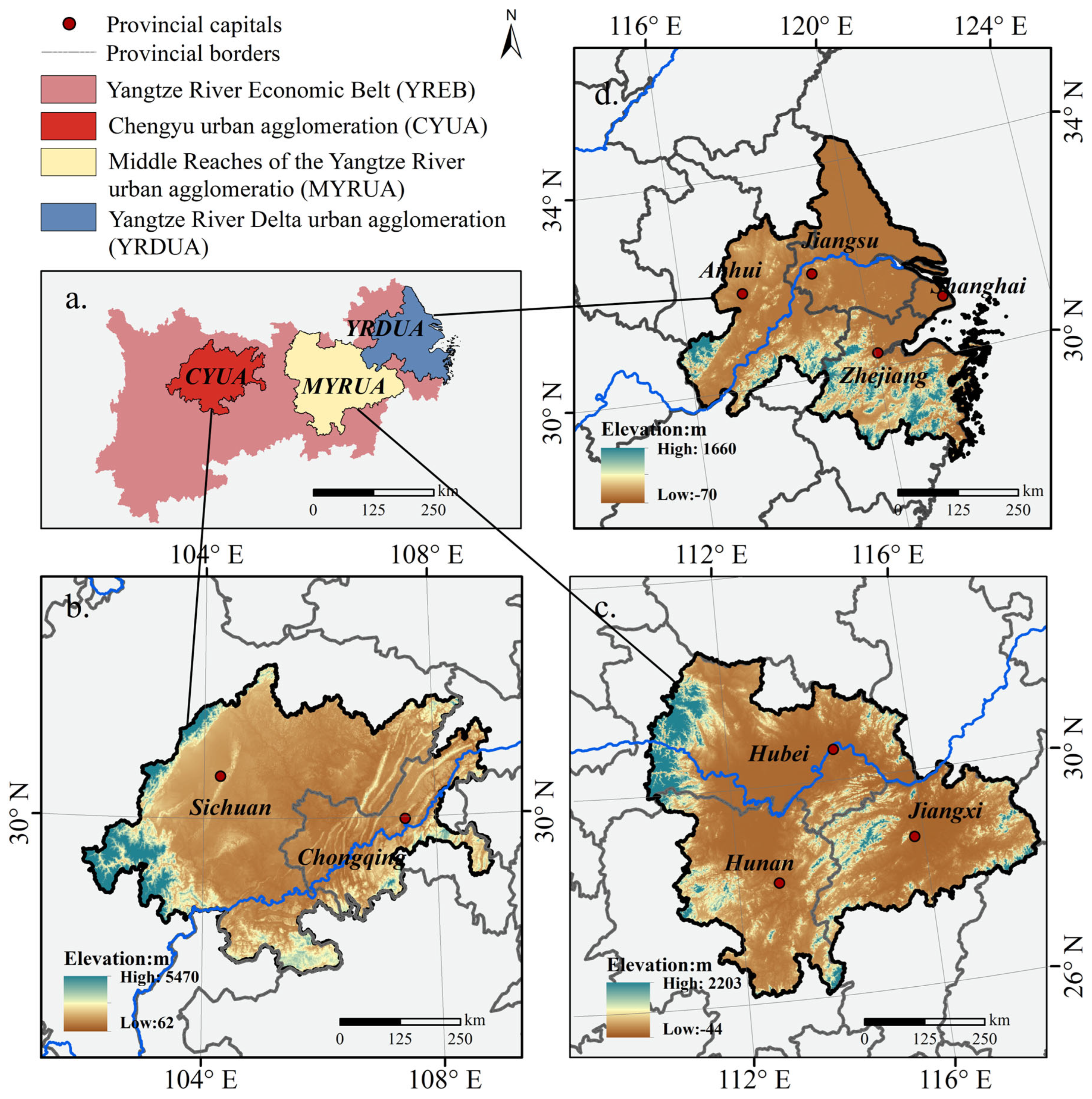
The three major urban agglomerations within the YREB (Figure 1) span latitudes from 26°03′ to 34°30′ north and longitudes from 101°57′ to 122°56′ east. These regions are among the most economically developed and dynamic in China, acting as key engines for future economic growth [43]. The urban agglomerations within the YREB display a wide range of geographical characteristics, encompassing the Sichuan Basin, the middle and lower reaches of the Yangtze River Plain, and China’s two largest freshwater lakes, Poyang Lake and Dongting Lake. Leveraging their advantageous topography, these urban agglomerations have attracted significant population inflows, resulting in rapid urbanization. By 2020, the three major urban agglomerations within the YREB collectively had a population of over 600 million people, accounting for 41.9% of China’s population. The region covers approximately 814,000 km2, or 8.5% of the country’s total land area, and its gross regional product reached 36.3 trillion yuan, contributing to 36.6% of China’s gross domestic product (GDP), all within less than 10% of the national territory. The urbanization rates in the CYUA, MRYUA, and YRDUA were 25.7%, 60.5%, and 68.4%, respectively, reflecting a high level of urbanization in China. However, the accelerating pace of urbanization is placing increasing strain on the EH of the YREB. Rapid UE has led to the compression and fragmentation of the region’s once-rich ecosystems, particularly in terms of the protection of wetlands, lakes, and forests. Issues such as water quality degradation, wetland loss, and declining forest cover are becoming more pronounced, posing significant threats to ecosystem services and biodiversity. For instance, the extent of wetlands in the Yangtze River Delta, forest cover in the Sichuan Basin, and water availability in the Yangtze River Basin are all on the decline [44]. As such, understanding the correlation between UE and EH, and finding a sustainable balance between the two, has become an urgent issue that must be addressed.

2.2. Data Sources

To comprehensively assess the impact of UE on EH, this study utilized land-use data from 2010 and 2020, derived from the GlobeLand30 dataset (https://www.webmap.cn/commres.do?method=globeIndex, accessed 4 December 2025). Using the GlobeLand30 products and incorporating the classification standards of the Chinese Academy of Sciences, the land-use data was reclassified into seven categories: cultivated land, forest, grassland, wetland, water bodies, artificial surfaces, and bareland. This study focused on the development of the YREB urban agglomerations, identifying key drivers from three dimensions: socioeconomic status, natural conditions, and accessibility. Elevation data were obtained from the ASTER GDEM 30 m product (https://search.earthdata.nasa.gov/, accessed 4 December 2025), which was subsequently assembled and clipped as required. Slope data were then computed from the elevation dataset. Population density data were sourced from WorldPop (https://hub.worldpop.org, accessed 4 December 2025). Geospatial information, including railways, highways (including expressways), water bodies, and municipal government locations, was extracted from the 1:1,000,000 public edition of the Basic Geographic Information Database (https://www.webmap.cn/, accessed 4 December 2025). Additionally, data on soil type, GDP, annual average precipitation, and annual average temperature were sourced from the Resource and Environmental Science Data Center of the Chinese Academy of Sciences (https://www.resdc.cn, accessed 4 December 2025). The locations of temples and train stations were retrieved from the OpenStreetMap (OSM) dataset (https://www.openstreetmap.org, accessed 4 December 2025). The normalized difference vegetation index (NDVI) was derived from the MODIS dataset, specifically accessed through Google Earth Engine and downloaded from NASA’s EarthData search portal (https://search.earthdata.nasa.gov/, accessed 4 December 2025). For consistency, all datasets were resampled to a resolution of 100 m to ensure uniformity and facilitate subsequent analyses (see Table 1).

2.3. Method

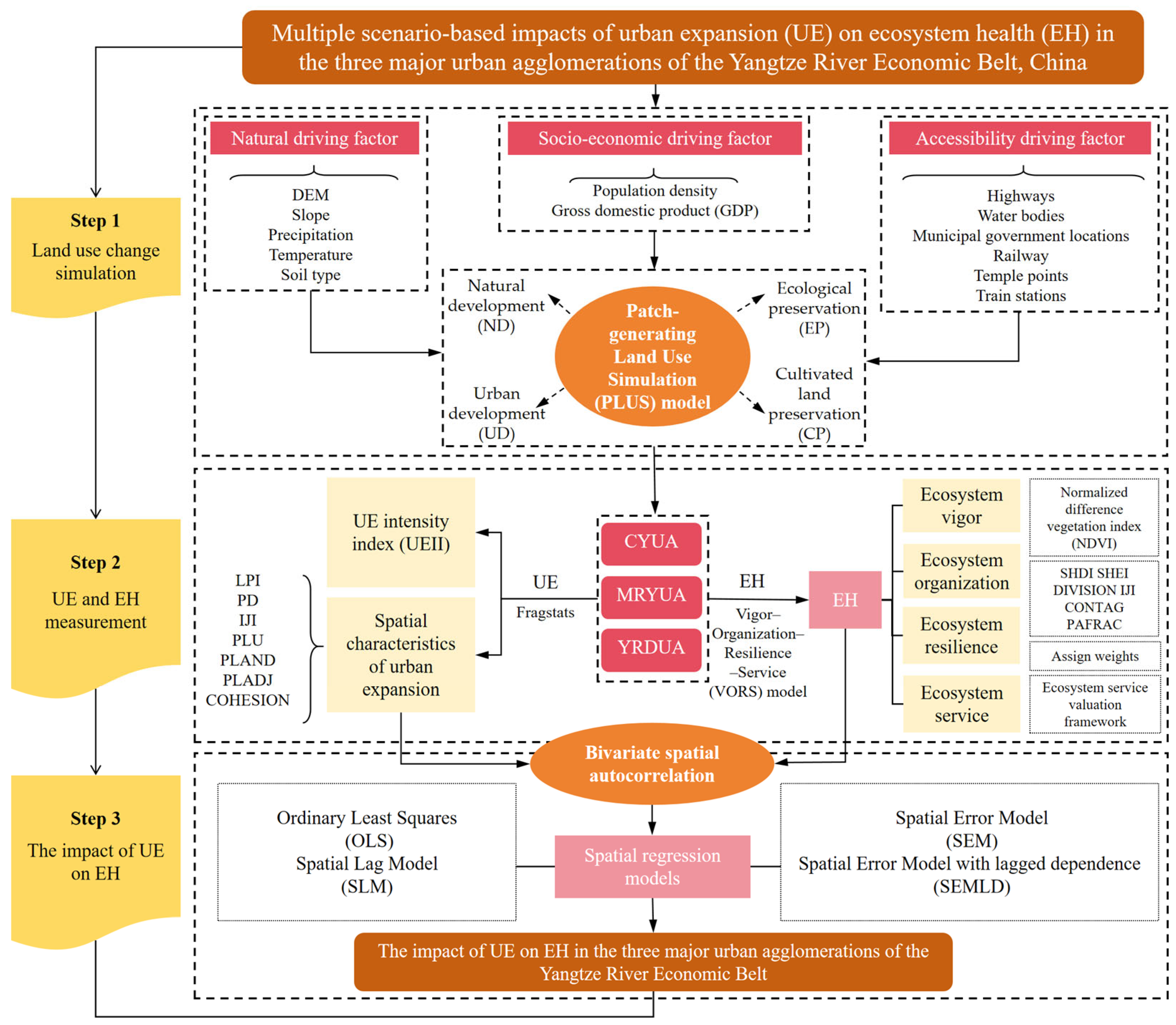
This study employs a systematic research methodology that encompasses data preparation, model construction, and spatial analysis to comprehensively examine the impact of UE in the three major urban agglomerations of the YREB on EH. The overall technical framework is illustrated in Figure 2 and consists of three primary steps. Firstly, land use simulation under multiple scenarios is conducted using the PLUS model, which integrates historical land use data with various driving factors to project land use changes in 2030 under four scenarios. Secondly, the measurement of UE and EH is carried out. The UE component is characterized mainly by UE intensity and spatial characteristics, employing the urban expansion intensity index (UEII) alongside a series of landscape pattern indices to quantify both the intensity and spatial morphology of UE. EH is assessed primarily based on the VORS model, which constructs a 10 km grid-scale EH from four dimensions: vitality, organizational capacity, resilience, and service function, in order to evaluate the EH status under different scenarios. Finally, the study applies bivariate spatial autocorrelation methods to analyze the spatial correlation between various UE indicators and EH. Furthermore, a series of spatial regression models are utilized to identify the pathways and intensity of the impact of UE on EH. Through these steps, the study systematically reveals the spatial mechanisms by which UE affects EH, providing a scientific basis for the sustainable development of the three major urban agglomerations in the YREB.

2.4. Land Use Simulation

The PLUS model is an advanced tool for predicting land-use change, which integrates rule mining techniques from land expansion analysis with a cellular automata model that incorporates a multi-type stochastic seeding mechanism [19]. This model simulates the spatiotemporal dynamics of land-use evolution by constructing area demand constraints and pixel-based transition probabilities under multiple policy scenarios. It includes a land expansion analysis strategy module to analyze land use changes over different time intervals. By integrating key factors and applying the random forest algorithm, the model identifies the drivers behind each type of land use expansion and estimates the development probability for various land uses, considering the influence of these factors on the expansion of each category. The model then utilizes the cellular automata framework with multiclass stochastic patch seeds and incorporates distinct neighborhood weights, transition matrices, and Markov-predicted future land class quantities to predict future land use changes.

2.4.1. Selection of Simulation Driving Factors

Land use change is influenced by various factors, which must be carefully selected for analysis within the PLUS model. Focusing on the development of urban agglomerations in the YREB, this study identifies key factors from three perspectives: socio-economic status, natural conditions, and accessibility. Specifically, the natural dimension includes elevation, slope, average annual precipitation, soil type, and average annual temperature. The socio-economic dimension covers population density and GDP density. Accessibility is assessed based on proximity to railways, highways (including expressways), water bodies, municipal government offices, train stations, and temples. In total, thirteen factors are identified as key drivers influencing the likelihood of urban agglomerations development along the YREB.

2.4.2. PLUS Model Parameter Settings

To explore multiple future development scenarios, the model referred to previous studies and categorized the simulated land use changes into four scenarios [20,45,46], as outlined in Table 2: natural development (ND), ecological preservation (EP), urban development (UD), and cultivated land preservation (CP). The ND scenario is based on the natural evolution of land use structure from 2010 to 2020; the UD scenario focuses on ensuring economic growth and meeting urban land demand, promoting urbanization through enhanced infrastructure; the EP scenario aims to safeguard natural reserves, woodlands, water bodies, and other ecologically critical lands, ensuring biodiversity and environmental quality, with improving ecological benefits as its core objective; while the CP scenario emphasizes strict control over the scale of basic farmland to prevent urban expansion from encroaching on agricultural land, thereby securing national food safety.
In a multi-scenario framework, land use changes are assigned domain weights across various scenarios. These domain weights reflect the priority for the allocation of land categories. They are inherently distributed based on comprehensive probabilities and proportional representation [46]. The allocation of domain weights is carried out in accordance with the specific scenario types, as outlined in Table 3.

2.4.3. Model Accuracy Check

Before simulating land use changes, it is crucial to validate the accuracy of the simulation results. Current research commonly uses the Kappa coefficient and the figure of merit (FOM) value for this validation [19]. A simulation is generally considered highly accurate when the Kappa coefficient exceeds 0.75 and the FOM value surpasses 0.1. In this study, the land use changes for the year 2020 were simulated and compared with actual data. The Kappa coefficient was found to be 0.751, and the FOM value was 0.116, indicating that the results meet the required accuracy standards.

2.5. UE Measurement

2.5.1. UEII Measurement

This study aims to explore the impact of UE on EH, with a focus on the spatiotemporal dimension of UE and quantifying its extent. To measure the intensity of UE, the UEII is employed. This index standardizes UE across different time periods, thereby capturing its temporal characteristics [47,48]. The specific equation is as follows:
U E I I = ( U e n d U s t a r t ) T L A × T × 100 %
where UEII is UE intensity index, Uend (Ustart) is the end (start) of the artificial surface area, T is the year of the interval, TLA is the total land use area.

2.5.2. Spatial Characteristics of UE

This study employed landscape patterns to describe the spatial characteristics of UE [49,50]. Specifically, we utilized percentage of artificial surfaces use (PLU), the largest patch index (LPI), patch density (PD), proportion of like adjacencies (PLADJ), patch cohesion index (COHESION), percentage of landscape (PLAND), and interspersion juxtaposition index (IJI) as indicators of UE landscape patterns [51]. These landscape indices are appropriate choices for studying UE, as they effectively reveal the aggregation, fragmentation, and extent of land use during the UE process [52]. The above landscape pattern indices were calculated by the moving window method using Fragstats 4.2 software, based on land use data for each year [53].

2.6. EH Assessment

Sustainable and stable EH can be derived from three aspects: vigor, organization, and resilience [46]. Based on this, combined with ecosystem services, the VORS model is established to evaluate EH. According to the framework constructed by this model, and in conjunction with existing studies [9], the equation can be obtained:
E H = E V × E O × E R × E S 4
where EV is ecosystem vigor, EO is ecosystem organization, ER is ecosystem resilience, ES is ecosystem services.
When calculating the EH, it is necessary to normalize the four indicators involved in the equation to eliminate the influence of different units among data indicators. The specific equation is as follows:
y n o r = x s e l f x m i n x m a x x m i n
where ynor is normalized values in the range [0, 1], xself is the value of the indicator itself, xmin and xmax are the minimum and maximum values within the indicator.
To access the EH of the three major urban agglomerations in the YREB, this study employed a grid-based approach to ensure uniformity and equity in evaluating EH. The study area was segmented into grids, with the three major urban agglomerations distributed across these units. The grid resolution is 10 km × 10 km. 7908 grid cells were obtained after removing outliers. Subsequent calculations of indicator values were all based on individual grid areas. To accurately differentiate the health status of ecosystems, the EH is subdivided into five levels: weak health (0–0.45), relatively weak health (0.45–0.55), ordinary health (0.55–0.65), good health (0.65–0.75), and excellent good health (0.75–1) [39].

2.6.1. Ecosystem Vigor Assessment

Ecosystem vigor is an indicator of the ecosystem’s resilience to external disturbances and serves as a direct reflection of its productive vigor. This vigor is frequently measured using the NDVI, which is a metric utilized for evaluating vegetation conditions. The NDVI can be applied for both qualitative and quantitative assessments of vegetation coverage and growth vigor [54,55]. Higher NDVI values indicate more robust plant growth, which corresponds to a more vigorous ecosystem. The calculation is as follows:
N D V I = N I R R E D N I R + R E D
where NDVI is the normalized difference vegetation index, NIR is the near-infrared band, and RED is the red band. The 2030 NDVI value was substituted with the 2020 value, so no separate comparison was made for vitality in multi-scenario analysis. When assessing multiple future scenarios, we observed minimal variation in NDVI values after averaging them across grid cells. Consequently, we utilized a uniform NDVI value for computational processing.

2.6.2. Ecosystem Organization Assessment

Ecosystem organization refers to the stability and complexity of ecosystems’ internal structures, typically evaluated using landscape pattern indices. Based on existing research and real-world scenarios [56,57], this study employed six landscape pattern indices to represent ecosystem organization: Shannon’s diversity index (SHDI), Shannon’s evenness index (SHEI), landscape division index (DIVISION), IJI, contagion index (CONTAG), and perimeter–area fractal dimension (PAFRAC). The SHDI and the SHEI are utilized to quantify the heterogeneity of a landscape, measuring its diversity. The IJI describes the overall distribution and adjacency of different patch types, reflecting the aggregation level of landscape patches. The CONTAG reveals the spreading tendency of the landscape, while the DIVISION indicates the dispersion level of landscape elements. The PAFRAC displays the complexity of landscape shapes. Based on existing research and practical scenarios, we have developed an assessment method for ecosystem organizational strength by assigning weights to various landscape pattern blocks. The specific equation is as follows:
O = 0.2 × S H D I + 0.2 × S H E I + 0.1 × D I V I S I O N + 0.15 × C O N T A G + 0.15 × I J I + 0.2 × P A F R A C
where O is ecosystem organization, SHDI is Shannon’s diversity index, SHEI is Shannon’s evenness index, DIVISION is landscape division index, CONTAG is contagion index, IJI is interspersion juxtaposition index, PAFRAC is perimeter–area fractal dimension.

2.6.3. Ecosystem Resilience Assessment

Ecosystem resilience is characterized by its capacity to revert to its initial state post-disturbance. This capability is intimately linked with land use and is primarily dictated by the specific attributes associated with such use. Therefore, building on previous research [9,58], we assigned weights to land use types, with weights of 0.5, 0.9, 0.6, 0.8, 0.8, 0.4, and 0.3 for cultivated land, forest, grassland, wetland, water bodies, artificial surfaces, and bareland, respectively.

2.6.4. Ecosystem Services Assessment

Ecosystem services encompass the direct or indirect benefits that ecosystems offer to humans, serving as a reference for human well-being [59]. The value of products and services that ecosystems offer to society through their functions can serve as a means to measure the output of ecological services from ecosystem [60]. This study built upon the ecosystem services valuation framework established by Costanza and integrated the value equivalence table developed by Xie [34,61]. It refines and categorizes various types of ecosystem services based on empirical data and related research [25,34]. Subsequently, based on the optimized ecosystem services weight table (Table 4), this study evaluated the potential by aligning land use types with their corresponding ecosystem services.

2.7. Bivariate Spatial Autocorrelation

The bivariate spatial autocorrelation analysis can unveil the correlation between two variables at a spatial level [62,63]. In this study, we employed the bivariate spatial autocorrelation method to investigate the relationship between UE and EH [20]. We analyzed the spatial correlation between EH and the indicator of UE by calculating the global Moran’s I and local Moran’s I of the indicators of the two variables [64]. The equations for the calculations are as follows:
I g l o b a l = n i = 1 n j 1 n W i j E H j e U E x j u ( n 1 ) i = 1 n j 1 n W i j
I l o c a l = E H i e j = 1 n W i j U E x j u
where W i j is the weight connection matrix of i and j, E H j e   a n d   U E x are the EH and indicator of UE, and n is the number of grids.

2.8. Spatial Regression Model

This study employed a spatial regression model to examine the impact of UE on EH. Spatial regression analysis quantifies the relationship between a dependent variable and one or more independent variables across geographic spaces, while accounting for spatial dependencies among observations [65,66]. According to the first law of geography, spatial data often exhibit autocorrelation, which violates the independence assumption of traditional regression models. Spatial regression models address this spatial dependence, yielding more accurate estimates of the relationships between variables.
Commonly used spatial regression models include Ordinary Least Squares (OLS), Spatial Lag Model (SLM), Spatial Error Model (SEM), and Spatial Error Model with lagged dependence (SEMLD) [66]. The general forms of these models are as follows:
O L S :   Y = X β + ε
S L M :   Y = ρ X Y + X β + ε
S E M :   Y = X β + u ,   w h e r e   u = λ W u + ε
S E M L D :   Y = ρ W Y + X β + W Y θ + ε
where Y is the dependent variable (EH in this study), X is the matrix of independent variables (including UE), β is the vector of regression coefficients, ε is the error term, W is the spatial weights matrix, ρ is the spatial autoregressive coefficient, λ is the spatial error coefficient, θ is the vector of coefficients for the spatially lagged independent variables.
Initially, we conducted a spatial regression analysis across the entire urban agglomerations of the YREB to identify the most suitable model. Following this, the selected model was applied to separate analyses of the three major urban agglomerations. By integrating spatial effects, the chosen model offers more accurate estimates of the impact of UE on EH, while accounting for the spatial interdependencies inherent within urban and ecological systems.

3. Results

3.1. Multi-Scenario Simulation of Land Use Change

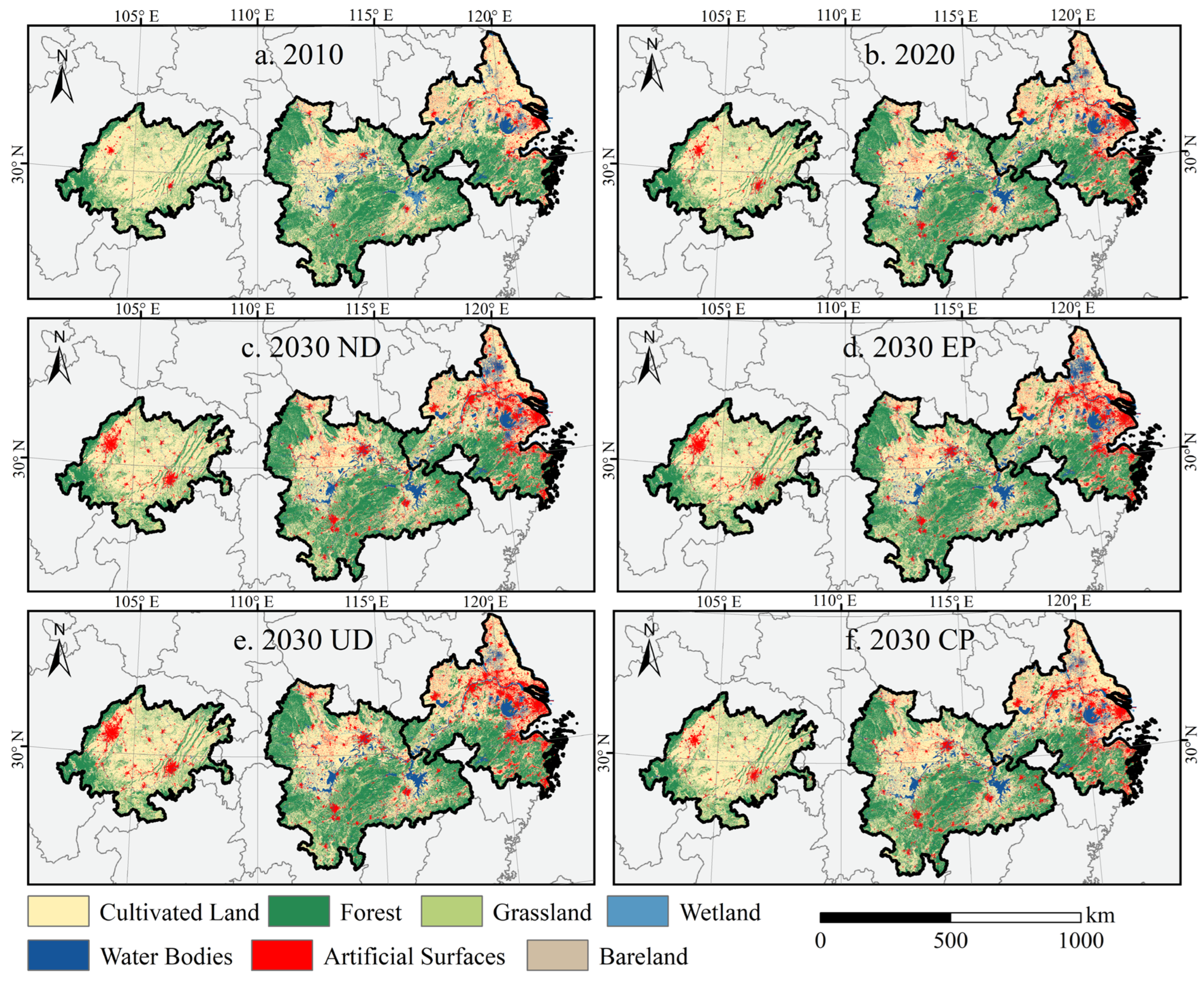
The results from the PLUS model indicated a significant expansion of artificial surfaces across various simulation scenarios, with the most pronounced growth observed in provincial capital cities (Figure 3). This substantial increase in artificial surfaces reflects clear trends in UE, as detailed in Table S1. Under the ND, EP, UD, and CP scenarios, the rates of increase in artificial surfaces were 35.34%, 33.22%, 44.77%, and 24.57%, respectively. These findings suggest that both the EP and CP scenarios have the potential to moderate the pace of UE.
Each scenario revealed unique aspects of land use alterations. In the UD scenario, UE was the fastest, with the greatest loss of ecological land, especially wetland, which was reduced by 33.98%. Conversely, the CP scenario exhibited the slowest rate of UE, and it was the only scenario in which the area of cultivated land saw a slight increase (0.26%). The EP scenario, while controlling UE, also contributed to the protection and restoration of ecological land, such as forest and grassland, which showed slight increases, while the area of water bodies grew significantly by 8.90%. It is important to note that wetland consistently showed a declining trend, particularly in the urban development and urban renewal scenarios, where wetland were reduced most drastically—by 33.98% and 22.71%, respectively—emphasizing the urgent need for wetland conservation.
Spatially, the most notable feature of land-use changes from 2010 to 2020, as well as in multi-scenario projections through to 2030, was the ongoing process of urbanization. Artificial surface areas consistently expanded across all periods and scenarios, with a more pronounced increase in the eastern and central regions. This expansion primarily occurred at the expense of cultivated land, reflecting urbanization’s encroachment on agricultural land. Although the overall area of forest cover remained relatively stable, some regions experienced slight declines, likely due to UE and the growing demand for other land uses. Notably, the areas of water bodies and wetland remained relatively unchanged across all periods and scenarios, which may indicate the successful implementation of water resource management and ecological conservation policies. Furthermore, the study revealed distinct regional disparities, showing that the rate and extent of urbanization in the eastern regions were considerably greater than in the western and central regions. The 2030 projections for the different scenarios further illustrated potential land-use change trajectories, with artificial surface expansion being most pronounced in the UD scenario.
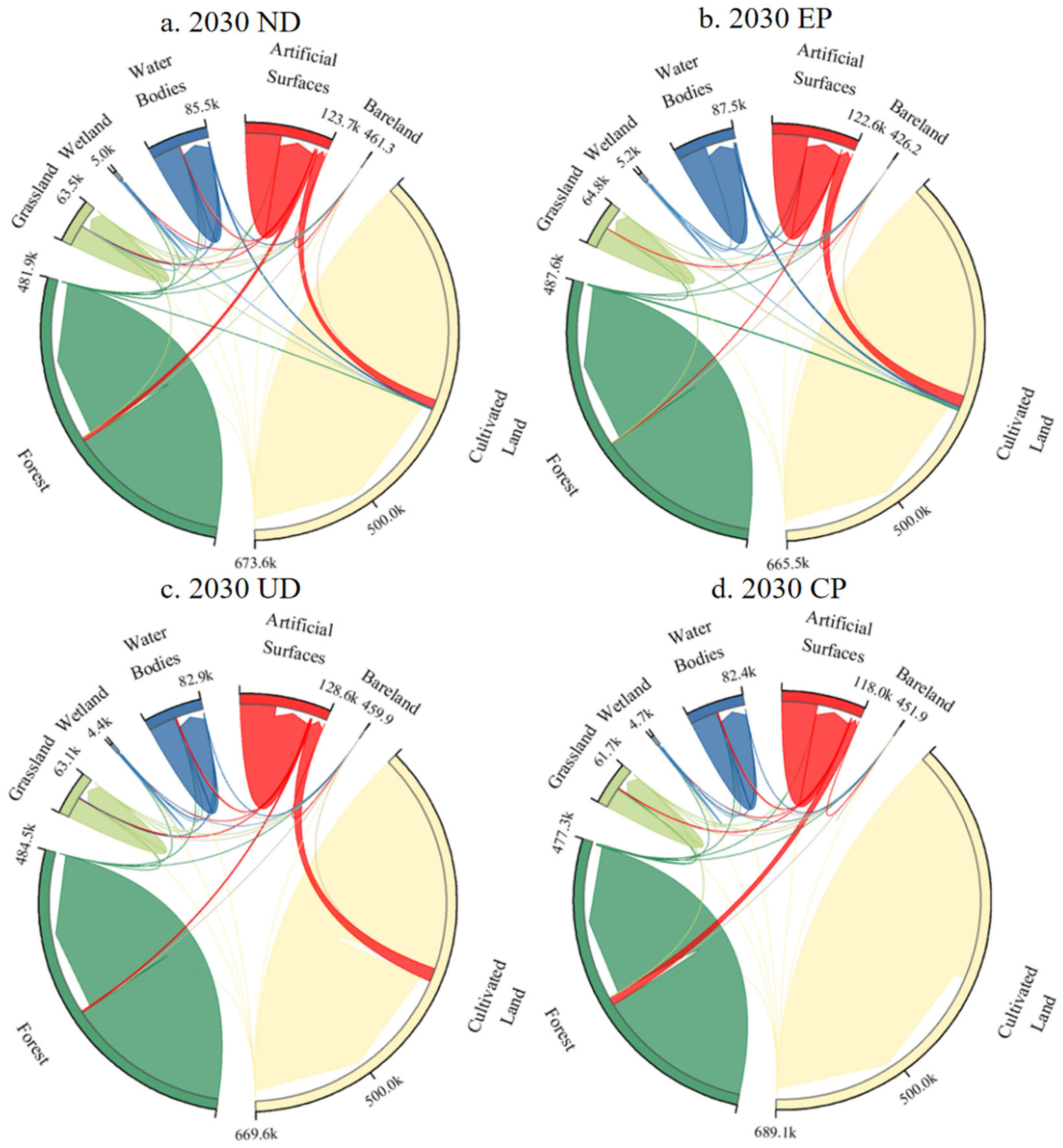
In the context of land-use changes projected for 2030, Figure 4 presents a Sankey diagram based on the land-use change matrix from 2020 to 2030. Compared to the ND scenario, the EP scenario effectively limited the conversion of forest and grassland to other land uses, thus preserving the integrity of green landscapes. Under the CP scenario, the extent of cultivated land remained relatively stable, although artificial surfaces encroached more onto green spaces, such as forest and grassland, resulting in a 6.79% conversion of green areas to artificial surfaces, marking a 5.57% increase over the ND scenario. In the UD scenario, the encroachment of artificial surfaces onto cultivated land was further exacerbated, reaching 5.60%, representing the highest level of cultivated land conversion among the four scenarios.

3.2. Landscape Character of UE

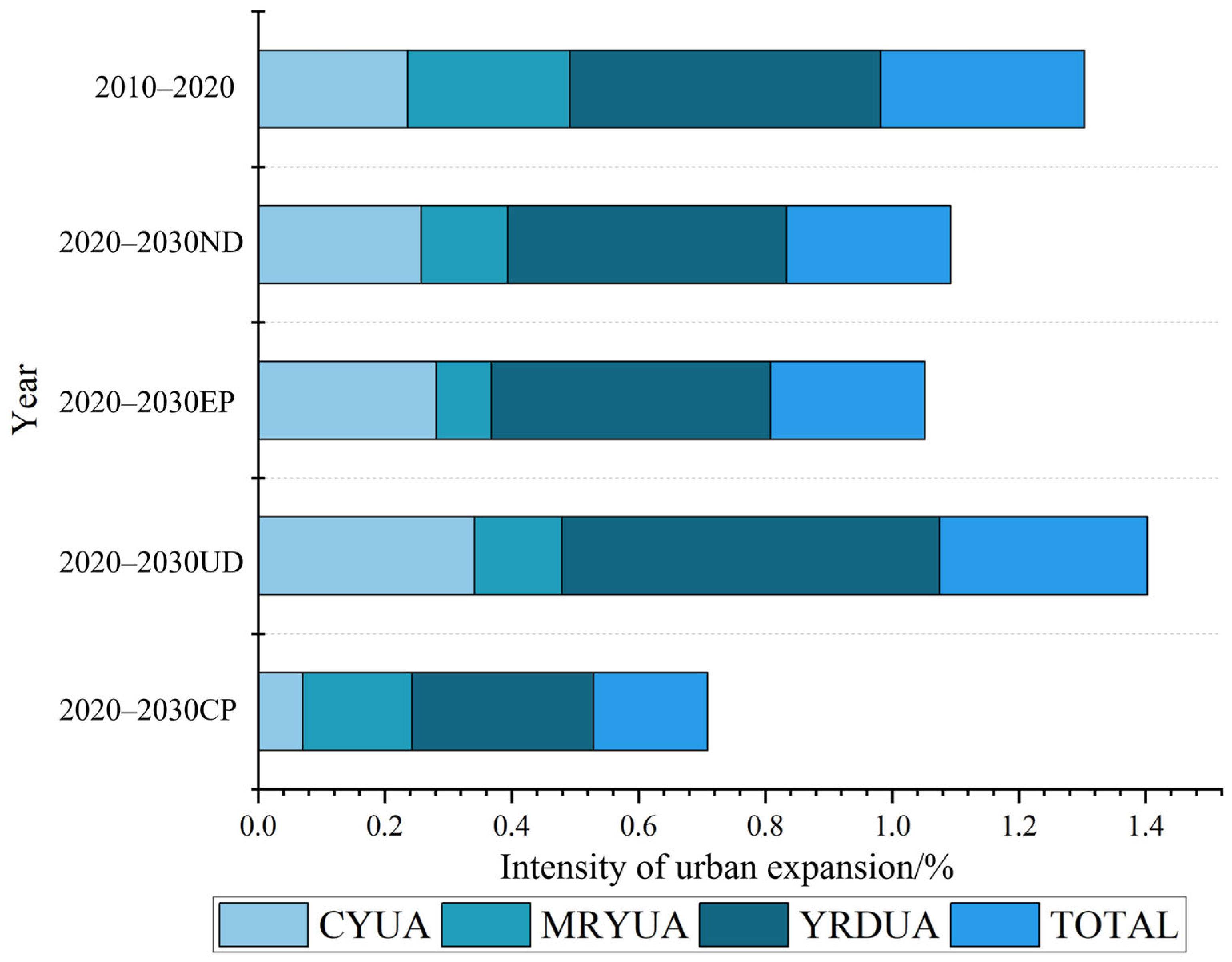
The UEII exhibited variations across different urban agglomerations (Figure 5). Positive development of U within three major urban agglomerations of the YREB is attributed to the continuous increase in urban land use. Future scenario analyses revealed diverse trends. Under the ND scenario, UEII in the CYUA increased to 0.26%, while that in the MRYUA decreased to 0.14%. The UEII in the YRDUA remained relatively stable at 0.44%, with the overall expansion intensity maintaining at 0.26%. In the EP scenario, UEII in CYUA increased further to 0.28%, while in MRYUA, it experienced a significant decline to 0.09%. UEII in YRDUA remained unchanged at 0.44%, with the overall expansion intensity slightly decreasing to 0.24%. Under the UD scenario, UEII in CYUA further increased to 0.34%, while MRYUA remained stable at 0.14%. Notably, the UEII in YRDUA rose significantly to 0.60%, and the overall expansion intensity also increased to 0.33%. In the CP scenario, UEII across all regions remained relatively low, particularly in CYUA, where the UEII was only 0.07%.
Landscape indices displayed notable differences across the three scenarios (Table S2). The LPI increased from 0.1826 in 2010 to 0.2103 in 2020, and is projected to continue rising across all scenarios by 2030. This suggests an expansion in the largest artificial surface patches, reflecting the ongoing process of UE. The PD generally increased from 0.1295 in 2010 to 2030, especially under the EP and UD scenarios, indicating a rise in the fragmentation of artificial surfaces. The PLADJ remained relatively high across all scenarios, rising from 78.9317 in 2010 to 81.8991 in 2020, with only slight changes projected for 2030. This indicates that the edge complexity of artificial surfaces is stabilizing at a certain level. COHESION remained close to 100 across all scenarios, demonstrating a high degree of cohesion in artificial surface use, with a slight increase over time. The IJI showed a marked increase from 2010 to 2030, particularly under the CP scenario, indicating an enhancement in the diversity and proximity of various land use types. Under all scenarios, the PLAND significantly increased from 2010 to 2030, reflecting the rising proportion of artificial surfaces in the total area, and indicating the progression of urbanization. The PLU reflected the share of artificial surfaces within the entire urban agglomerations, showing a consistent upward trend.

3.3. EH Changes in Multiple Scenarios

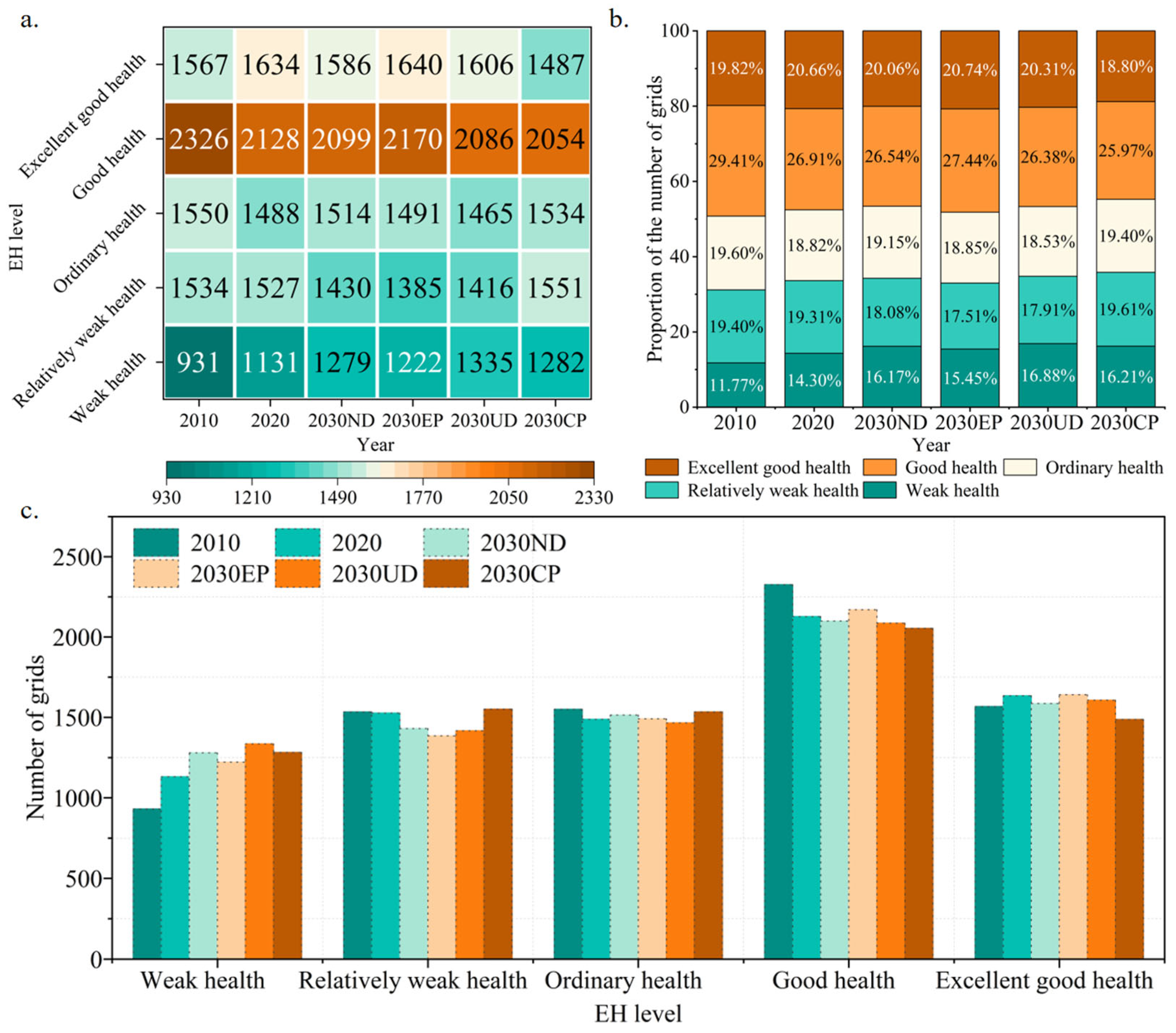
EH in the study area showed a declining trend, decreasing from an average of 0.621 in 2010 to 0.613 in 2020. Under four future simulated scenarios, the EH further declined, reaching 0.607 in the ND scenario, 0.612 in the EP scenario, and 0.605 and 0.604 under the UD and CP scenarios, respectively. In the weak health category, the number of grids increased from 931 in 2010 to 1131 in 2020 and reached 1335 under the 2030 UD scenario, clearly demonstrating the persistent deterioration trend of this category (Figure 6a). In the relatively weak health category, the number of grids slightly decreased from 1534 in 2010 to 1527 in 2020, with future scenarios showing divergence: a decline in ND and UD scenarios and an increase in EP and CP scenarios, reaching 1551 in the CP scenario, reflecting the complexity of this category influenced by different driving factors. The number of grids in the ordinary health category decreased from 1550 in 2010 to 1488 in 2020, with overall downward fluctuations in future scenarios, particularly dropping to 1465 in the UD scenario, indicating sustained pressure on the ecosystems. The number of grids in the good health and excellent health categories significantly declined between 2010 and 2020 but rebounded in all scenarios except the CP scenario by 2030, with the most notable recovery observed in the EP scenario. Good health consistently represents the highest proportion, although it shows a gradual declining trend (Figure 6b). In contrast, the proportion of excellent good health remains relatively stable, fluctuating between 18% and 21%. The combined proportions of weak health and relatively weak health have long been maintained at 30% to 35%, indicating that nearly one-third of the regions are in a vulnerable state. The differences in proportions among various scenarios for 2030 further corroborate this trend differentiation. For instance, in the UD scenario, the proportion of excellent good health is the highest, while it is the lowest in the CP scenario, intuitively reflecting the impact of different development pathways on the health structure of the ecosystem. The number of grids classified as good health is consistently the highest across all years and scenarios, peaking in the 2030 UD scenario, which underscores its dominant position (Figure 6c). The number of grids classified as weak health has steadily increased from 2010 to 2020; however, it experiences a decline in all scenarios for 2030. Additionally, the fluctuations in the number of grids classified as relatively weak health and ordinary health correspond to the trend differentiation revealed in Figure 6a, collectively indicating that the future improvement or deterioration of EH will be highly dependent on the choice of developmental scenarios.
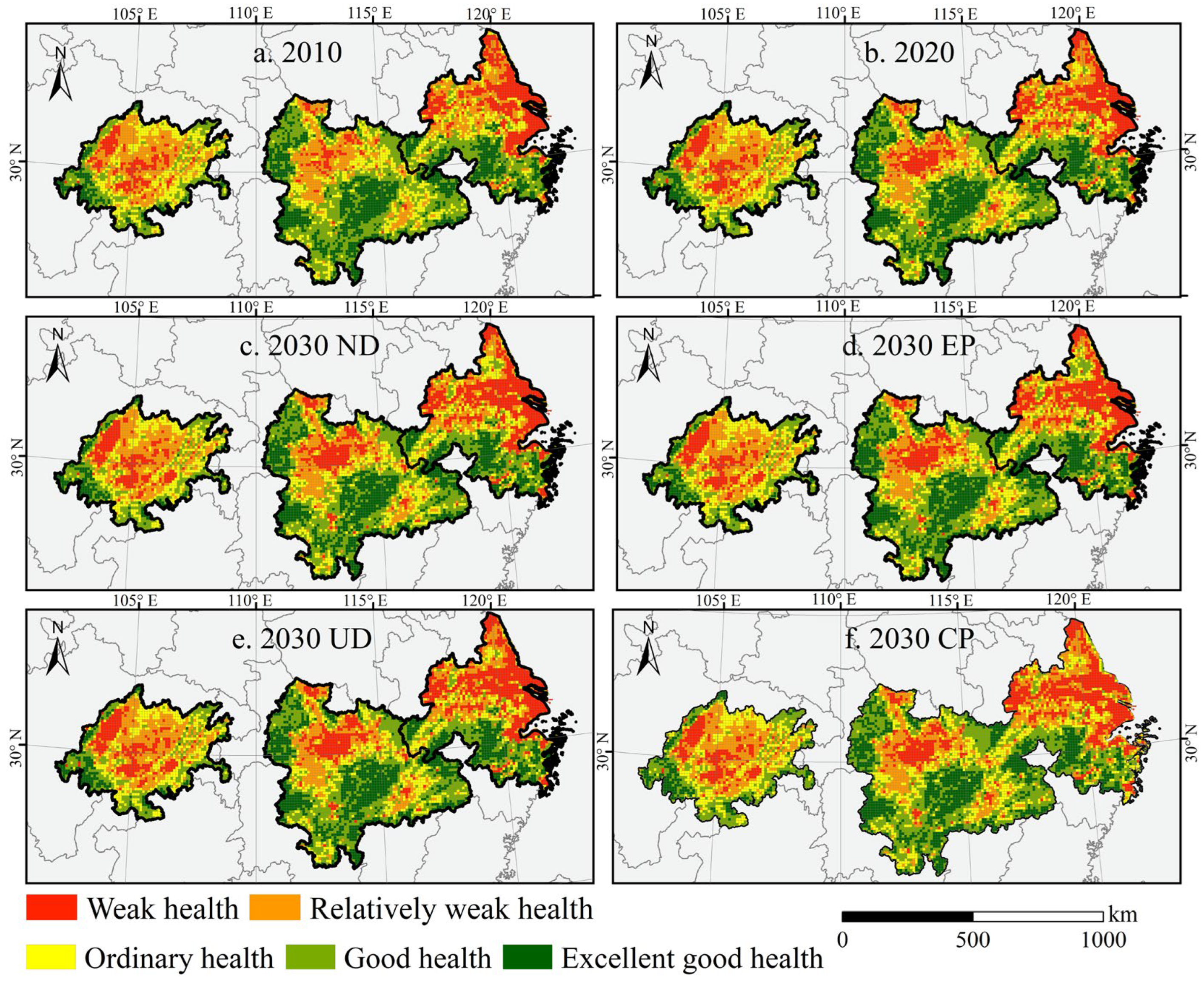
Across the three urban agglomerations, there was a general decline in EH (Figure 7). The CYUA, located in the Sichuan Basin with predominantly cultivated land, exhibited a relatively fragile ecosystem, making it more susceptible to the impacts of UE. The deterioration of EH was most pronounced in areas extending outward from the central cities of Chengdu and Chongqing. In contrast, the regions around Leshan and Ya’an, characterized by mountainous terrain and dense vegetation cover, maintained a more stable EH. In the MRYUA, the Jianghan Plain, particularly in Tianmen, Qianjiang, and Xiantao, showed significant degradation in EH. Although the EH levels in Wuhan, Changsha, and Nanchang were also on a declining trend, the changes were less pronounced. The Mufu Mountains and Luoxiao Mountain, however, preserved higher levels of EH, owing to less impact from UE. The YRDUA, exhibiting the highest level of urban development, also contained many regions with low EH, particularly along the Yangtze River and in areas near Hangzhou Bay and Tai Lake. In future development scenarios, EH along the Yangtze River continued to decline, largely due to urbanization and the ongoing expansion and fragmentation of cultivated land and artificial surfaces. However, the Dabie Mountain region maintained a high level of EH, owing to its high altitude and challenging terrain, which limited development.

3.4. Spatial Autocorrelation Between EH and UE

The Bivariate spatial autocorrelation analysis (Table S3) revealed a consistently negative correlation between each UE indicator and EH at the grid scale, with statistically significant results. This indicates a significant spatial association between the urbanization process and variations in EH. Specifically, as UE progresses, EH tends to decline within the spatial context. Over time, with the exception of the CP scenario, the global Moran’s I index for the seven UE indicators in relation to EH decreased, indicating an intensification of the negative correlation between them. Consequently, the UE process appears to pose a significant threat to EH.
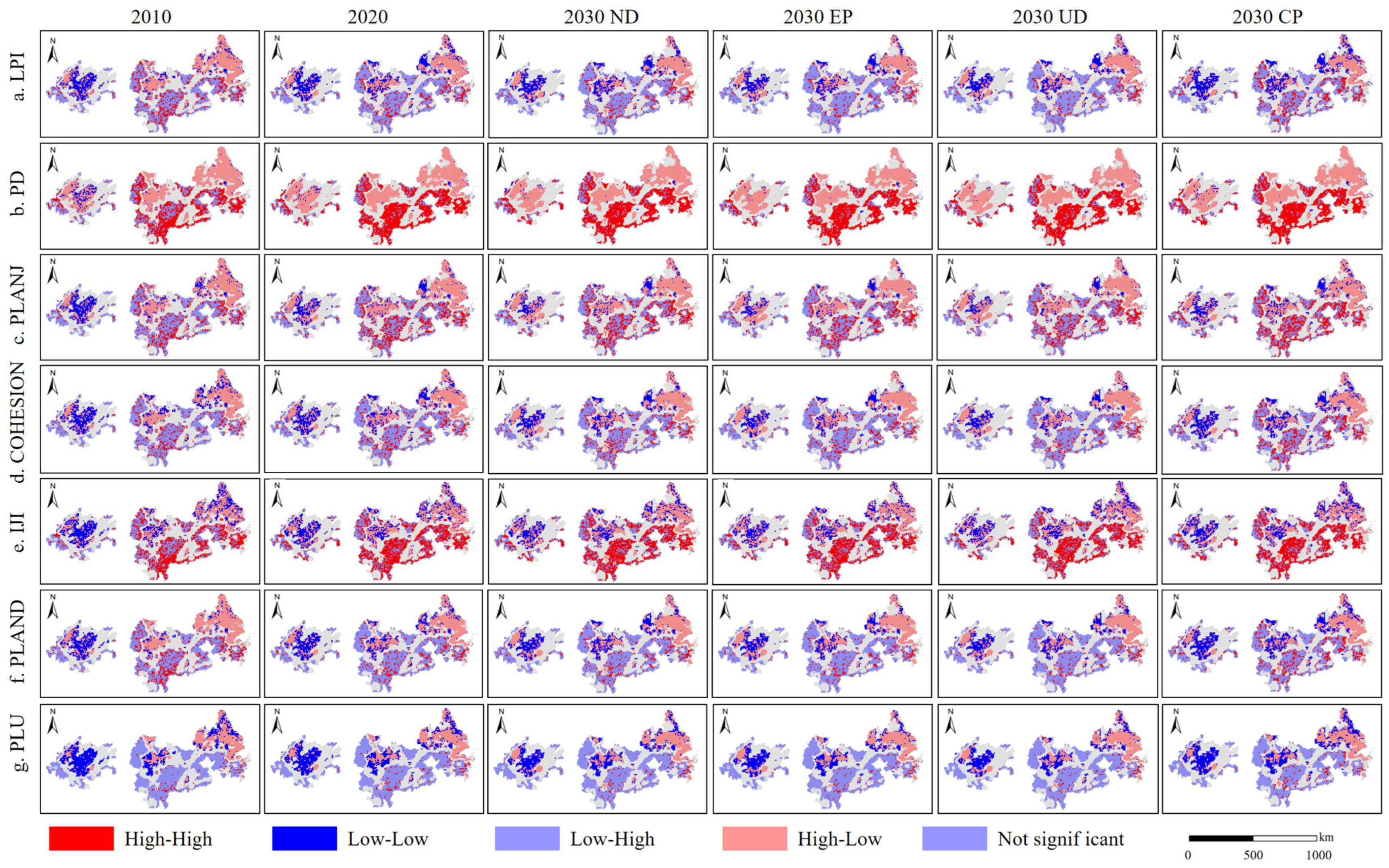
The high- and low-value clustering characteristics of the three urban agglomerations differed significantly (Figure 8). In the central Sichuan Basin, clusters of high–low (high PD, low EH), low–low (low LPI, low EH), low–low (low PLADJ, low EH), low–low (low COHESION, low EH), low–low (low IJI, low EH), low–low (low PLAND and low EH), and low–low (low PLU, low EH) are observed. In contrast, mountainous regions such as the Dabie, Mufu, Luoxiao, and Wuling Mountains predominantly exhibited low–high (low LPI, high EH), low–high (low PLU, high EH), high–high (high PD, high EH) and high–high (high IJI, high EH). Meanwhile, PLADJ, COHESION, and PLAND showed a mixed pattern of high–high and low–low clusters. In highly urbanized areas such as the middle and lower reaches of the Yangtze River Plain, Chengdu Plain, Jianghan Plain, cities like Changsha and Nanchang, there is a prevalence of high–low (high LPI, low EH), high–low (high PD, low EH), high–low (high PLADJ, low EH), high–low (high COHESION, low EH), high–low (high PLAND, low EH), and high–low (high PLU, low EH). However, the IJI showed an intermingled distribution of both low–low and high–low clusters. The central area of the CYUA, located in the west, exhibited numerous low–low aggregations. This suggested a high degree of landscape fragmentation, with more homogeneous patch types and lower connectivity and aggregation, resulting in poorer EH. In contrast, the mountainous region of the central MRYUA, characterized by higher topographic complexity and greater biodiversity, displayed smaller patch sizes but strong connectivity between them, ensuring the continuity of ecological processes and contributing to better EH. Conversely, the plains areas of MRYUA and YRDUA exhibited high urbanization, leading to greater fragmentation and reduced EH. Overall, the results indicate that UE is strongly negatively correlated with EH when compared to regions with little urbanization.

3.5. Impact of UE on EH

The OLS regression analysis did not account for the spatial dependence between UE and EH. Consequently, we further applied spatial regression models, deriving from the OLS test. Among the spatial regression models, the SLM and the SEM were utilized in this study to analyze the impacts of UE on EH across three urban agglomerations. The SLM and SEM models based on Queen’s spatial weights fitted well, with R2 ranging from 0.62 to 0.78, where the SEM model fitted slightly better. Among the factors affecting EH, PLU showed the most significant and consistent negative correlation, with coefficients ranging from −0.1955 to −0.3498, implying that land planning plays a crucial role in EH. PD also generally showed a significant negative correlation, suggesting that landscape fragmentation may be detrimental to EH. The IJI demonstrated consistent positive correlations, though the coefficients were small (0.0003–0.0009), implying that landscape complexity may have a minor positive effect on EH. The direction of the effects for most variables remained stable across different projections from 2010 to 2030, although the intensity of these effects varied. Notably, the impacts of the LPI and the PLAND became less significant in the 2030 UD scenario, reflecting the complexity of ecosystem dynamics during urbanization. Spatial effects were significant in both models. The coefficients for the lag term in the SLM model (0.5921–0.6524) and the coefficients for the error term in the SEM model (0.8206–0.8348) were both positive and highly significant, strongly supporting the existence of notable spatial dependence and spillover effects between UE and EH.
Based on the analysis, this study chose the SEM for further spatial regression analysis (Table 5 and Table 6). The results of the spatial regression analysis reveal the key mechanisms and regional differences through which UE impacts EH. The differentiated effects of landscape pattern indicators on EH are significant, with PLU and PD demonstrating the most pronounced negative impacts, while IJI shows a weak positive effect. This result reflects the core disturbance to ecosystems caused by land fragmentation resulting from UE. There is heterogeneity in the responses of the three major urban agglomerations. The YRDUA exhibits the strongest correlation between UE and EH, while the CYUA is least disturbed under the CP scenario. In contrast, the mountainous areas of the MRYUA maintain better ecological stability due to topographical constraints. The widespread existence of spatial dependence and spillover effects validates that the impact of UE on EH is not confined to localized areas but rather encompasses inter-regional ecological connections, providing crucial evidence for collaborative regional ecological governance.

4. Discussion

4.1. Agglomeration of Findings

This study revealed a significant negative spatial association and spillover effects between UE and EH within the three major urban agglomerations of the YREB, thereby validating and deepening our understanding of a critical dilemma within China’s rapid urbanization process. On a national scale, the research conducted by Wei et al. (2024) indicates that rapid construction land expansion from 2000 to 2020 has facilitated an overall improvement in EH [66]. However, it has simultaneously exacerbated spatial inequalities within economic regions and urban agglomerations [66]. This provides a crucial macro context for our findings: the local degradation observed at the urban agglomerations level is likely a specific manifestation of the intensifying internal inequalities. In other words, the average EH of the urban agglomerations may obscure the severe degradation occurring in its core expansion areas, which is precisely what our grid-scale analysis has uncovered. Furthermore, our spatial econometric model confirms a strong spatial dependence (significant Lambda coefficient), which directly resonates with the “significant spatial spillover effects” highlighted by the studies of Wei et al. (2024) and Zhang et al. (2024) [66,67]. The convergence of multiple lines of evidence suggests that the ecological impacts of UE are inherently transboundary. This shifts policy concerns from isolated degradation “hotspots” to the integrity and connectivity of regional ecological networks, indicating that destruction in one area may undermine the ecological resilience of neighboring regions.
Chen et al. (2024) provide a macro-contextual analysis of the Yangtze River Basin, revealing an overall improvement in EH across the basin, while persistent hotspots of degradation remain in regions such as the Sichuan Basin and the Yangtze River Delta [55]. Our study specifically focuses on these identified hotspots, elucidating the concrete processes (multi-scenario UE) and direct mechanisms (changes in landscape indices such as PLU and PD) that lead to such localized degradation, thereby bridging macro-level assessments with mechanistic explanations. The stark contrast between the severe degradation of EH in the YRDUA and the relatively mitigated impacts in the CYUA can be interpreted through the lens of regional inequality driving factors. Wei et al. (2024) found that rapid construction land expansion exacerbates EH inequality in the eastern regions while alleviating it in the central and western areas [66]. This macro-pattern reveals our micro-level findings: as a core region in eastern China, the UE in the Yangtze River Delta is not only large in scale but also highly concentrated, leading to intense spatial competition and profound ecological fragmentation. In contrast, the Chengdu–Chongqing region, influenced by the dynamics of western development and basin topography, may exhibit a different expansion pattern, where new construction land does not always directly conflict with the highest-value ecological land, potentially resulting in a relatively equal, albeit still negative, impact.
This study analyzes a series of landscape pattern indicators, revealing the multi-dimensional pathways through which UE affects EH. First, UE directly erodes ecological integrity by altering the proportional representation of land use types. The PLU emerges as the most significant negative factor; its increase directly signifies the irreversible replacement of ecologically high-value lands such as forests, grasslands, wetlands, and water bodies. This process not only directly undermines the vitality and organization of ecosystems but also leads to a fundamental decline in the capacity of ecosystem services. Research by Peng et al. (2023) confirms that land use change is a core driving force behind the loss of ecosystem services [59]. In this study, the UD scenario reveals that the more intense UE leads to a more significant negative growth in EH, providing strong evidence for this pathway. Secondly, the landscape fragmentation induced by UE systematically damages the resilience and connectivity of ecosystems. An increase in the PD signifies a worsening of habitat fragmentation, which can obstruct species migration and gene flow, severing the material and energy links necessary for ecological processes, thereby weakening the recovery capacity of ecosystems following disturbances [68]. Concurrently, indicators such as COHESION and IJI contribute positively to EH. This finding aligns with the conclusion of Yaermaimaiti et al. (2024), which asserts that the complexity and connectivity of landscape patterns play a critical role in maintaining ecological functions [57]. Therefore, the impact of UE on EH largely depends on whether it exacerbates fragmentation while weakening or preserving critical landscape connectivity. Consequently, future ecological management policies should not only focus on the minimum quantitative thresholds for ecological land use but should also prioritize the maintenance and optimization of “pattern quality” in landscapes. This can be achieved by protecting key ecological patches and constructing ecological corridors to actively optimize connectivity indicators like IJI, thereby enhancing the overall resilience and stability of regional ecosystems.

4.2. Policy Implications

Trend analysis and multi-scenario simulations suggest that UE is an irreversible trend that could accelerate if left unregulated. The impact of UE on EH is becoming increasingly evident, making the need to address the relationship between UE and EH more urgent. China’s sustainable development strategy aims to strike a balance between urbanization and ecological preservation, promoting ecological, economic, and social benefits. However, a more detailed division of urban agglomerations planning is still necessary [67,69,70].
According to the findings of this study, EH is significantly affected by UE. To mitigate the ecological damage caused by UE, priority should be given to strengthening the planning and management of ecological reserves, particularly in key ecological areas such as wetlands, forests, and rivers, during the urbanization process. This includes guiding urban agglomerations to expand in an orderly and concentrated manner, delineating UE boundaries, and establishing ecological land use boundaries. The optimal direction for expansion should be identified through multi-scenario simulations of land use, ensuring a balance between ecological protection and urban development. Special ecological zones, such as the major freshwater lakes (Poyang Lake and Dongting Lake) in the MYRUA, should have tailored land use strategies that prioritize maintaining the region’s ecological structure [68,71].
For regions with fragile EH, targeted restoration policies should be formulated, and existing resources should be rationally utilized to establish a safe and sustainable ecological pattern [72,73,74]. Within urban agglomerations, the establishment of eco-parks and eco-corridors can help maintain ecological balance while promoting green building practices, such as rain gardens and urban greening initiatives [75,76,77]. At the same time, it is important to focus on improving land use efficiency, reducing unnecessary UE, advocating for the redevelopment of existing urban spaces, and promoting vertical development [41,47,78]. For urban agglomerations, strengthening regional synergy and coordinating development efforts is essential. This includes planning for the factors that impact EH, ensuring that the development of various urban agglomerations aligns with ecological environmental protection, and optimizing the spatial structure for integrated governance and environmental management [79,80,81].

4.3. Limitations and Future Direction

This study, while striving for rigor, does have several limitations. First and foremost, the timeliness and consistency of the data are primary constraints. Due to the updating cycle of high-precision publicly available land use data, the reference year for this research is set to 2020, while more recent comprehensive data (e.g., for 2025) are not yet available. To ensure the accuracy and authority of the driving factor data, some spatial data (such as railway and water systems) utilize the 2021 version, which is closer to the reference year. Although this aims to enhance simulation accuracy, and the model validation results (Kappa = 0.751) support the reasonableness of this approach, minor discrepancies due to differences in data sources across years remain an unavoidable limitation. Secondly, the model’s predictions are based on the assumption that current environmental conditions and policy enforcement are relatively stable, which failed to adequately incorporate long-term dynamic uncertainties such as climate change and socioeconomic fluctuations that may impact the robustness of long-term forecasts. Lastly, the quantification of social perception dimensions, such as cultural services, in the assessment of EH remains somewhat simplified. Moreover, the spatial regression model primarily captures global linear relationships, thus having limited capabilities in revealing complex nonlinear responses and spatial heterogeneity mechanisms. To address these limitations, future research could expand in the following directions. Once more unified and timely datasets become available, the simulation results can be further validated and updated. Additionally, the research could attempt to couple climate and socioeconomic composite scenarios to enhance the dynamic nature of predictions. It could also integrate multi-source perception data to improve the assessment framework, and employ methods such as geographically weighted regression and machine learning to delve deeper into the spatial non-stationarity and nonlinear characteristics of influencing mechanisms. This would provide a more adaptable scientific basis for the sustainable development of urban agglomerations in various regions.

5. Conclusions

This study integrates the PLUS model and the VORS model to conduct multi-scenario simulations and spatial econometric analyses of UE and its impact on EH within the three major urban agglomerations of the YREB (the YRDUA, the MRYUA, and the CYUA). The multi-scenario simulations indicated that UE will continue until 2030, displaying significant scenario-based and regional variations. YRDUA exhibits the strongest expansion (with an artificial surface area increase of 44.77% under the UD scenario), while UE in the MRYUA slows down under both the EP and CP scenarios. The CYUA region shows the weakest expansion in the CP scenario (with an UEII of only 0.07%). The expansion is primarily characterized by the outward spread from core cities, encroaching upon cultivated land and ecological areas. From 2010 to 2020, overall EH declined (with the EH decreasing from 0.621 to 0.613), showcasing significant spatial differentiation. The degradation of EH is most pronounced in YRDUA, with areas of low EH in the MRYUA concentrated in the Jianghan Plain. The CYUA region exhibits a pattern of “core degradation and peripheral stability” in terms of EH. In future scenarios for 2030, the downward trend in EH will persist under the ND and UD scenarios, while both the EP and CP scenarios may alleviate this decline. Spatial analysis reveals a significant negative spatial dependence relationship between UE and EH. Bivariate spatial autocorrelation indicates that urban landscape indicators and EH are significantly negatively correlated across the three urban agglomerations, with YRDUA showing the highest absolute value of global Moran’s I, implying the strongest spatial clustering effect. The spatial error model further uncovers that PLU is the most consistently negative factor affecting EH. PD also generally exerts negative impacts, whereas the IJI contributes slightly positively to EH. This research systematically explores the ecological effects of UE, from process prediction to mechanism analysis, particularly revealing gradient differences and heterogeneous mechanisms in the intensity and spatial patterns among the three urban agglomerations. It provides a basis for formulating differentiated spatial governance policies. However, the study has limitations, such as insufficient consideration of climate and policy dynamics, a relatively simplistic assessment of cultural services, and a predominance of linear assumptions in the models. Future research could couple climate–social scenarios, integrate multi-source data to enhance service assessments, and employ geographic weighted regression or machine learning techniques to identify non-linear mechanisms, thereby facilitating more refined spatial decision-making.

Supplementary Materials

The following supporting information can be downloaded at: https://www.mdpi.com/article/10.3390/land15020330/s1. Table S1. Multi-scenario modeling of land use change in 2030; Table S2. Changes of UE indicators in 2010, 2020, and 2030 in each scenario; Table S3. Bivariate global Moran’s I of EH and UE in 2010, 2020, and 2030 in each scenario.

Author Contributions

L.Z., Z.L., J.W. (Jiahui Wu), W.Z., J.W. (Jianpeng Wang) and Y.P.: Methodology, Writing—original draft, Resources; Z.L.: Conceptualization, Supervision; Z.L., L.Z., J.W. (Jianpeng Wang), J.W. (Jiahui Wu), W.Z. and Y.P.: Writing—review and editing; Z.L., L.Z., J.W. (Jiahui Wu), W.Z. and Y.P.: Software, Data curation. All authors have read and agreed to the published version of the manuscript.

Funding

This work was supported by the project of Changjiang Survey, Planning, Design and Research Co., Ltd. [CX2022Z23]. The project was also supported by the Key Laboratory of Geospatial Technology for Middle and Lower Yellow River Regions (Henan University), Ministry of Education (No. GTYR202205).

Data Availability Statement

Dataset available on request from the authors.

Acknowledgments

The authors would like to thank the anonymous reviewers for their constructive comments on improving this paper.

Conflicts of Interest

Authors Liang Zheng and Jianpeng Wang were employed by the Changjiang Survey, Planning, Design and Research Co., Ltd. The remaining authors declare that the research was conducted in the absence of any commercial or financial relationships that could be construed as a potential conflict of interest. The authors declare that this study received funding from Changjiang Survey, Planning, Design and Research Co., Ltd. The funder was not involved in the study design, collection, analysis, interpretation of data, the writing of this article or the decision to submit it for publication.

Abbreviations

UE: Urban Expansion; YREB: Yangtze River Economic Belt; EH: Ecosystem Health; PLUS: Patch-generating Land Use Simulation; VORS: Vigor–Organization–Resilience–Service; YRDUA: Yangtze River Delta Urban Agglomerations; MRYUA: Middle Reaches of the Yangtze River Urban Agglomerations; CYUA: Chengdu–Chongqing Urban Agglomerations; ND: Natural Development; EP: Ecological Preservation; UD: Urban Development; CP: Cultivated Land Preservation; FOM: Figure of Merit; UEII: Urban Expansion Intensity Index; PLU: Percentage of Artificial Surfaces Use; LPI: Largest Patch Index; PD: Patch Density; PLADJ: Proportion of Like Adjacencies; COHESION: Patch Cohesion Index; PLAND: Percentage of Landscape; IJI: Interspersion Juxtaposition Index; SHDI: Shannon’s Diversity Index; SHEI: Shannon’s Evenness Index; DIVISION: Landscape Division Index; CONTAG: Contagion Index; PAFRAC: Perimeter–Area Fractal Dimension.

References

  1. Wang, J.; Chen, Y.; Liao, W.; He, G.; Tett, S.F.; Yan, Z.; Zhai, P.; Feng, J.; Ma, W.; Huang, C.; et al. Anthropogenic emissions and urbanization increase risk of compound hot extremes in cities. Nat. Clim. Change 2021, 11, 1084–1089. [Google Scholar] [CrossRef] [Scilit]
  2. Li, G.; Fang, C.; Watson, J.E.; Sun, S.; Qi, W.; Wang, Z.; Liu, J. Mixed effectiveness of global protected areas in resisting habitat loss. Nat. Commun. 2024, 15, 8389. [Google Scholar] [CrossRef] [Scilit] [PubMed]
  3. Zhou, G.; Eisenhauer, N.; Terrer, C.; Eldridge, D.J.; Duan, H.; Guirado, E.; Berdugo, M.; Zhou, L.; Liu, S.; Zhou, X.; et al. Resistance of ecosystem services to global change weakened by increasing number of environmental stressors. Nat. Geosci. 2024, 17, 882–888. [Google Scholar] [CrossRef] [Scilit]
  4. Gao, J.; Bukovsky, M.S. Urban land patterns can moderate population exposures to climate extremes over the 21st century. Nat. Commun. 2023, 14, 6536. [Google Scholar] [CrossRef] [Scilit]
  5. Iqbal, M.; Arshed, N.; Chan, L.F. Exploring the dynamics: Biodiversity impacts of natural resource extraction with moderating influence of FinTech for sustainable practices in resource-rich nations. Resour. Policy 2024, 91, 104933. [Google Scholar] [CrossRef] [Scilit]
  6. Baccour, S.; Goelema, G.; Kahil, T.; Albiac, J.; van Vliet, M.T.; Zhu, X.; Strokal, M. Water quality management could halve future water scarcity cost-effectively in the Pearl River Basin. Nat. Commun. 2024, 15, 5669. [Google Scholar] [CrossRef] [Scilit] [PubMed]
  7. Li, G.; Fang, C.; Li, Y.; Wang, Z.; Sun, S.; He, S.; Qi, W.; Bao, C.; Ma, H.; Fan, Y.; et al. Global impacts of future urban expansion on terrestrial vertebrate diversity. Nat. Commun. 2022, 13, 1628. [Google Scholar] [CrossRef] [Scilit]
  8. Testi, I.; Wang, A.; Paul, S.; Mora, S.; Walker, E.; Nyhan, M.; Duarte, F.; Santi, P.; Ratti, C. Big mobility data reveals hyperlocal air pollution exposure disparities in the Bronx, New York. Nat. Cities 2024, 1, 512–521. [Google Scholar] [CrossRef] [Scilit]
  9. Chen, W.; Gu, T.; Xiang, J.; Luo, T.; Zeng, J.; Yuan, Y. Ecological restoration zoning of territorial space in China: An ecosystem health perspective. J. Environ. Manag. 2024, 364, 121371. [Google Scholar] [CrossRef] [Scilit]
  10. Yuan, Y.; Chen, W.; Zeng, J.; Gu, T. Spatiotemporal evolution patterns and driving mechanisms of global ecosystem health. Geogr. Res. 2025, 44, 2626–2642. (In Chinese) [Google Scholar] [CrossRef]
  11. Ahmad, Y.; Zahra, R.; Ali, C. Transformations in urban gardens: Neoliberal influences and land use conflicts in Shiraz’s Qasr al-Dasht Gardens. Land Use Policy 2024, 146, 107311. [Google Scholar] [CrossRef] [Scilit]
  12. Barau, A.S.; Maconachie, R.; Ludin, A.N.M.; Abdulhamid, A. Urban morphology dynamics and environmental change in Kano, Nigeria. Land Use Policy 2015, 42, 307–317. [Google Scholar] [CrossRef] [Scilit]
  13. Qu, Y.; Zhan, L.; Wei, C.; Zhang, Q.; Wang, J. Interactive transition of cultivated land and construction land during China’s urbanization: A coordinated analytical framework of explicit and implicit forms. Land Use Policy 2024, 138, 107049. [Google Scholar] [CrossRef] [Scilit]
  14. Colsaet, A.; Laurans, Y.; Levrel, H. What drives land take and urban land expansion? A systematic review. Land Use Policy 2018, 79, 339–349. [Google Scholar] [CrossRef] [Scilit]
  15. Li, G.; Sun, S.; Fang, C. The varying driving forces of urban expansion in China: Insights from a spatial-temporal analysis. Landsc. Urban Plan. 2018, 174, 63–77. [Google Scholar] [CrossRef] [Scilit]
  16. Liu, P.; Hu, Y.; Jia, W. Land use optimization research based on FLUS model and ecosystem services–setting Jinan City as an example. Urban Clim. 2021, 40, 100984. [Google Scholar] [CrossRef] [Scilit]
  17. Pan, Z.; He, J.; Liu, D.; Wang, J. Predicting the joint effects of future climate and land use change on ecosystem health in the Middle Reaches of the Yangtze River Economic Belt, China. Appl. Geogr. 2020, 124, 102293. [Google Scholar] [CrossRef] [Scilit]
  18. Roy, B.; Rahman, M.Z. Spatio-temporal analysis and cellular automata-based simulations of biophysical indicators under the scenario of climate change and urbanization using artificial neural network. Remote Sens. Appl.-Soc. Environ. 2023, 31, 100992. [Google Scholar] [CrossRef] [Scilit]
  19. Liang, X.; Guan, Q.; Clarke, K.C.; Liu, S.; Wang, B.; Yao, Y. Understanding the drivers of sustainable land expansion using a patch-generating land use simulation (PLUS) model: A case study in Wuhan, China. Comput. Environ. Urban Syst. 2021, 85, 101569. [Google Scholar] [CrossRef] [Scilit]
  20. Chen, W.; Wang, G.; Gu, T.; Fang, C.; Pan, S.; Zeng, J.; Wu, J. Simulating the impact of urban expansion on ecosystem services in Chinese urban agglomerations: A multi-scenario perspective. Environ. Impact Assess. Rev. 2023, 103, 107275. [Google Scholar] [CrossRef] [Scilit]
  21. Qiao, W.; Huang, X. The impact of land urbanization on ecosystem health in the Yangtze River Delta urban agglomerations, China. Cities 2022, 130, 103981. [Google Scholar] [CrossRef] [Scilit]
  22. Luan, C.; Liu, R.; Li, Y.; Zhang, Q. Comparison of various models for multi-scenario simulation of land use/land cover to predict ecosystem service value: A case study of Harbin-Changchun Urban Agglomeration, China. J. Clean. Prod. 2024, 478, 144012. [Google Scholar] [CrossRef] [Scilit]
  23. Yu, Z.; Yang, G.; Lin, T.; Zhao, B.; Xu, Y.; Yao, X.; Ma, W.; Vejre, H.; Jiang, B. Exposure ecology drives a unified understanding of the nexus of (urban) natural ecosystem, ecological exposure, and health. Ecosyst. Health Sustain. 2024, 10, 0165. [Google Scholar] [CrossRef] [Scilit]
  24. Yadav, A.; Kansal, M.L.; Singh, A. Ecosystem health assessment based on the VORS framework for the Upper Ganga Riverine Wetland in India. Environ. Sustain. Indic. 2025, 25, 100580. [Google Scholar] [CrossRef] [Scilit]
  25. Hernández-Blanco, M.; Costanza, R.; Chen, H.; DeGroot, D.; Jarvis, D.; Kubiszewski, I.; Montoya, J.; Sangha, K.; Stoeckl, N.; Turner, K.; et al. Ecosystem health, ecosystem services, and the well-being of humans and the rest of nature. Glob. Change Biol. 2022, 28, 5027–5040. [Google Scholar] [CrossRef] [Scilit] [PubMed]
  26. Lin, X.; Wang, Z.; Bao, Y. Integrating ecosystem stress into the assessment of ecosystem health in karst areas and exploring its driving factors. Ecol. Indic. 2024, 167, 112662. [Google Scholar] [CrossRef] [Scilit]
  27. Liu, X.; Han, Y.; Li, Y.; Li, L.; Liu, Y. Evaluation of ecosystem health improvement potential based on “water-based”: Taking the Chahannaoer basin of Inner Mongolia Autonomous Region as an example. Acta Ecol. Sin. 2025, 45, 2868–2876. (In Chinese) [Google Scholar] [CrossRef]
  28. Ma, J.; Tian, L.; Zhang, Y.; Yang, X.; Li, Y.; Liu, Z.; Zhou, L.; Wang, Z.; Ouyang, W. Global property rights and land use efficiency. Nat. Commun. 2024, 15, 8525. [Google Scholar] [CrossRef] [Scilit]
  29. Ma, X.; Tan, J. Study on the collaborative integration of ecosystem health and tourism resource development and its zonal management in Nanshan National Park. Acta Ecol. Sin. 2025, 45, 9408–9418. (In Chinese) [Google Scholar] [CrossRef]
  30. Wang, Y.; Xue, H.; Li, A.; Ma, X.; Sun, A.; Zhang, J. Spatial-temporal differentiation and influencing factors of ecosystem health in Three-River-Source national Park. Ecol. Indic. 2025, 171, 113183. [Google Scholar] [CrossRef] [Scilit]
  31. Heller, N.E.; McManus Chauvin, K.; Skybrook, D.; Barnosky, A.D. Including stewardship in ecosystem health assessment. Nat. Sustain. 2023, 6, 731–741. [Google Scholar] [CrossRef] [Scilit]
  32. Gunawan, H.; Setyawati, T.; Atmoko, T.; Subarudi; Kwatrina, R.T.; Yeny, I.; Yuwati, T.W.; Effendy, R.; Abdullah, L.; Mukhlisi; et al. A review of forest fragmentation in Indonesia under the DPSIR framework for biodiversity conservation strategies. Glob. Ecol. Conserv. 2024, 51, e02918. [Google Scholar] [CrossRef] [Scilit]
  33. Raj, A.; Sharma, L.K. Spatial E-PSR modelling for ecological sensitivity assessment for arid rangeland resilience and management. Ecol. Model. 2023, 478, 110283. [Google Scholar] [CrossRef] [Scilit]
  34. Costanza, R. Nature: Ecosystems without commodifying them. Nature 2006, 443, 749. [Google Scholar] [CrossRef] [Scilit] [PubMed]
  35. Wang, P.; Song, Y.; Zhang, J.; Yu, P.; Zhang, Y.; Zhang, X.; Wang, C. Research on factors affecting ecosystem health in Beijng-Tianjin-Hebei region and its multi-scenario simulation based on different spatial scales. Acta Ecol. Sin. 2025, 45, 8986–8999. (In Chinese) [Google Scholar] [CrossRef]
  36. Das, M.; Das, A.; Mandal, A. Research note: Ecosystem Health (EH) assessment of a rapidly urbanizing metropolitan city region of eastern India–A study on Kolkata Metropolitan Area. Landsc. Urban Plan. 2020, 204, 103938. [Google Scholar] [CrossRef] [Scilit]
  37. Sahana, M.; Saini, M.; Areendran, G.; Imdad, K.; Sarma, K.; Sajjad, H. Assessing Wetland ecosystem health in Sundarban Biosphere Reserve using pressure-state-response model and geospatial techniques. Remote Sens. Appl.-Soc. Environ. 2022, 26, 100754. [Google Scholar] [CrossRef] [Scilit]
  38. Kii, M. Projecting future populations of urban agglomerations around the world and through the 21st century. npj Urban Sustain. 2021, 1, 10. [Google Scholar] [CrossRef] [Scilit]
  39. Gu, T.; Luo, T.; Ying, Z.; Wu, X.; Wang, Z.; Zhang, G.; Yao, Z. Coupled relationships between landscape pattern and ecosystem health in response to urbanization. J. Environ. Manag. 2024, 367, 122076. [Google Scholar] [CrossRef] [Scilit] [PubMed]
  40. Han, P.; Hu, H.; Zhou, J.; Wang, M.; Zhou, Z. Integrating key ecosystem services to study the spatio-temporal dynamics and determinants of ecosystem health in Wuhan’s central urban area. Ecol. Indic. 2024, 166, 112352. [Google Scholar] [CrossRef] [Scilit]
  41. Wang, X.; Yao, W.; Luo, Q.; Yun, J. Spatial relationship between ecosystem health and urbanization in coastal mountain city, Qingdao, China. Ecol. Inform. 2024, 79, 102458. [Google Scholar] [CrossRef] [Scilit]
  42. Gourevitch, J.D.; Alonso-Rodríguez, A.M.; Aristizábal, N.; de Wit, L.A.; Kinnebrew, E.; Littlefield, C.E.; Moore, M.; Nicholson, C.C.; Schwartz, A.J.; Ricketts, T.H. Projected losses of ecosystem services in the US disproportionately affect non-white and lower-income populations. Nat. Commun. 2021, 12, 3511. [Google Scholar] [CrossRef] [Scilit]
  43. Zhai, M.; Wu, Y.; Gu, Y.; Su, S.; Zang, H.; Ding, W.; Lu, J. Development of an interactive multi-region enviro-economic equilibrium (IMR3E) model for managing inner-and inter-region carbon-emission mitigation. Resour. Conserv. Recycl. 2023, 199, 107214. [Google Scholar] [CrossRef] [Scilit]
  44. Tu, D.; Cai, Y.; Liu, M. Coupling coordination analysis and spatiotemporal heterogeneity between ecosystem services and new-type urbanization: A case study of the Yangtze River Economic Belt in China. Ecol. Indic. 2023, 154, 110535. [Google Scholar] [CrossRef] [Scilit]
  45. Scown, M.W.; Dunn, F.E.; Dekker, S.C.; Van Vuuren, D.P.; Karabil, S.; Sutanudjaja, E.H.; Santos, M.J.; Minderhoud, P.S.; Garmestani, A.S.; Middelkoop, H. Global change scenarios in coastal river deltas and their sustainable development implications. Glob. Environ. Change 2023, 82, 102736. [Google Scholar] [CrossRef] [Scilit]
  46. Zhao, C.; Wu, S.; Yang, L.; Wu, Y.; Xiao, P.; Xu, J.; Liu, Y. Evaluating ecological conservation effectiveness of security patterns under multiple scenarios: A case study of Hubei Province. Ecol. Indic. 2024, 166, 112528. [Google Scholar] [CrossRef] [Scilit]
  47. Ma, C.; Li, M.; Jiang, P. The multiscale response of global cropland cropping intensity to urban expansion. Agric. Syst. 2024, 221, 104138. [Google Scholar] [CrossRef] [Scilit]
  48. Schuster-Olbrich, J.P.; Marquet, O.; Miralles-Guasch, C.; Arce, L.F. Spatial patterns and drivers of urban expansion: An exploratory spatial analysis of the Metropolitan Region of Santiago, Chile, from 1997 to 2013. Cities 2024, 153, 105305. [Google Scholar] [CrossRef] [Scilit]
  49. Jung, M.C.; Wang, T.; Kang, M.; Dyson, K.; Dawwas, E.B.; Alberti, M. Urban landscape affects scaling of transportation carbon emissions across geographic scales. Sust. Cities Soc. 2024, 113, 105656. [Google Scholar] [CrossRef] [Scilit]
  50. Xing, X.; Shi, W.; Wu, X.; Liu, Y.; Wang, X.; Zhang, Y. Towards a more compact urban form: A spatial-temporal study on the multi-dimensional compactness index of urban form in China. Appl. Geogr. 2024, 171, 103368. [Google Scholar] [CrossRef] [Scilit]
  51. Chen, W.; Wang, G.; Zeng, J. Impact of urbanization on ecosystem health in Chinese urban agglomerations. Environ. Impact Assess. Rev. 2023, 98, 106964. [Google Scholar] [CrossRef] [Scilit]
  52. Anríquez, G.; Calabrese, J.; Foster, W.; Keim, K.; Osses, P. Refining the scale of the rural-urban landscape: A policy-relevant application to Chile. Appl. Geogr. 2024, 168, 103318. [Google Scholar] [CrossRef] [Scilit]
  53. Tian, Y.; Jim, C.Y.; Tao, Y.; Shi, T. Landscape ecological assessment of green space fragmentation in Hong Kong. Urban For. Urban Green. 2011, 10, 79–86. [Google Scholar] [CrossRef] [Scilit]
  54. Fang, W.; Huang, S.; Huang, Q.; Huang, G.; Wang, H.; Leng, G.; Wang, L.; Li, P.; Ma, L. Bivariate probabilistic quantification of drought impacts on terrestrial vegetation dynamics in mainland China. J. Hydrol. 2019, 577, 123980. [Google Scholar] [CrossRef] [Scilit]
  55. Chen, W.; Yuan, Y.; Liu, Z.; Zeng, J.; Yang, L.; Zhong, Y.; Gu, T.; Feng, Z. Ecosystem health in the Yangtze and Yellow River basins in China: Regional differences and driving forces. Ecol. Indic. 2024, 166, 112422. [Google Scholar] [CrossRef] [Scilit]
  56. Mallick, K.; Verfaillie, J.; Wang, T.; Ortiz, A.A.; Szutu, D.; Yi, K.; Kang, Y.; Shortt, R.; Hu, T.; Sulis, M.; et al. Net fluxes of broadband shortwave and photosynthetically active radiation complement NDVI and near infrared reflectance of vegetation to explain gross photosynthesis variability across ecosystems and climate. Remote Sens. Environ. 2024, 307, 114123. [Google Scholar] [CrossRef] [Scilit]
  57. Yaermaimaiti, A.; Li, X.; Ge, X.; Liu, C. Analysis of landscape pattern and ecological risk change characteristics in Bosten Lake basin based on optimal scale. Ecol. Indic. 2024, 163, 112120. [Google Scholar] [CrossRef] [Scilit]
  58. Zhang, J.; Wang, J.; Chen, Y.; Huang, S.; Liang, B. Spatiotemporal variation and prediction of NPP in Beijing-Tianjin-Hebei region by coupling PLUS and CASA models. Ecol. Inform. 2024, 81, 102620. [Google Scholar] [CrossRef] [Scilit]
  59. Peng, Y.; Chen, W.; Pan, S.; Gu, T.; Zeng, J. Identifying the driving forces of global ecosystem services balance, 2000–2020. J. Clean. Prod. 2023, 426, 139019. [Google Scholar] [CrossRef] [Scilit]
  60. Costanza, R.; De Groot, R.; Sutton, P.; Van der Ploeg, S.; Anderson, S.J.; Kubiszewski, I.; Farber, S.; Turner, R.K. Changes in the global value of ecosystem services. Glob. Environ. Change 2014, 26, 152–158. [Google Scholar] [CrossRef] [Scilit]
  61. Xie, G.; Zhang, C.; Zhang, L.; Chen, W.; Li, S. Improvement of the evaluation method for ecosystem service value based on per unit area. J. Nat. Resour. 2015, 30, 1243–1254. (In Chinese) [Google Scholar] [CrossRef]
  62. Dong, Y.H.; Peng, F.L.; Li, H.; Men, Y.Q. Spatial autocorrelation and spatial heterogeneity of underground parking space development in Chinese megacities based on multisource open data. Appl. Geogr. 2023, 153, 102897. [Google Scholar] [CrossRef] [Scilit]
  63. Legendre, P. Spatial autocorrelation: Trouble or new paradigm? Ecology 1993, 74, 1659–1673. [Google Scholar] [CrossRef] [Scilit]
  64. Dormann, C.F.; McPherson, J.M.; Araújo, M.B.; Bivand, R.; Bolliger, J.; Carl, G.; Davies, R.G.; Hirzel, A.; Jetz, W.; Kissling, W.D.; et al. Methods to account for spatial autocorrelation in the analysis of species distributional data: A review. Ecography 2007, 30, 609–628. [Google Scholar] [CrossRef] [Scilit]
  65. Al Kafy, A.; Dey, N.N.; Saha, M.; Altuwaijri, H.A.; Fattah, M.A.; Rahaman, Z.A.; Kalaivani, S.; Bakshi, A.; Rahaman, S.N. Leveraging machine learning algorithms in dynamic modeling of urban expansion, surface heat islands, and carbon storage for sustainable environmental management in coastal ecosystems. J. Environ. Manag. 2024, 370, 122427. [Google Scholar] [CrossRef] [Scilit]
  66. Wei, G.; He, B.J.; Liu, Y.; Li, R. How does rapid urban construction land expansion affect the spatial inequalities of ecosystem health in China? Evidence from the country, economic regions and urban agglomerations. Environ. Impact Assess. Rev. 2024, 106, 107533. [Google Scholar] [CrossRef] [Scilit]
  67. Zhang, F.; Xie, A.; Jiang, C.; Chen, J.; An, Y.; Yang, P.; Ma, D. Coupling coordination analysis and spatiotemporal heterogeneity between urban land green use efficiency and ecosystem services in Yangtze River Economic Belt, China. Hum. Soc. Sci. Commun. 2024, 11, 1328. [Google Scholar] [CrossRef] [Scilit]
  68. Li, Y.; Qin, L.; Wang, Y.; Liu, H.; Zhang, M.; Hao, H. Ecosystem health assessment of the largest lake wetland in the Yellow River basin using an improved vigor-organization-resilience-services model. Ecol. Indic. 2024, 166, 112539. [Google Scholar] [CrossRef] [Scilit]
  69. Chung, M.G.; Frank, K.A.; Pokhrel, Y.; Dietz, T.; Liu, J. Natural infrastructure in sustaining global urban freshwater ecosystem services. Nat. Sustain. 2021, 4, 1068–1075. [Google Scholar] [CrossRef] [Scilit]
  70. Eldridge, D.J.; Cui, H.; Ding, J.; Berdugo, M.; Sáez-Sandino, T.; Duran, J.; Gaitan, J.; Blanco-Pastor, J.L.; Rodríguez, A.; Plaza, C.; et al. Urban greenspaces and nearby natural areas support similar levels of soil ecosystem services. npj Urban Sustain. 2024, 4, 15. [Google Scholar] [CrossRef] [Scilit]
  71. Seidl, A.; Mulungu, K.; Arlaud, M.; van den Heuvel, O.; Riva, M. The effectiveness of national biodiversity investments to protect the wealth of nature. Nat. Ecol. Evol. 2021, 5, 530–539. [Google Scholar] [CrossRef] [Scilit]
  72. Liu, Y.; Liu, J.; Yin, X.; Ouyang, X.; Ji, C.; Li, S.; Wei, G. Human activities and ecosystem health: A historical analysis of Poyang Lake. Ecol. Indic. 2024, 166, 112446. [Google Scholar] [CrossRef] [Scilit]
  73. Luo, Q.; Zhou, J.; Zhang, Y.; Yu, B.; Zhu, Z. What is the spatiotemporal relationship between urbanization and ecosystem services? A case from 110 cities in the Yangtze River Economic Belt, China. J. Environ. Manag. 2022, 321, 115709. [Google Scholar] [CrossRef] [Scilit] [PubMed]
  74. Qu, H.; You, C.; Wang, W.; Guo, L. Spatio-temporal interplay between ecosystem services and urbanization in the Yangtze River Economic Belt: A new perspective for considering the scarcity effect. Land Use Policy 2024, 147, 107358. [Google Scholar] [CrossRef] [Scilit]
  75. Abdelaal, F.; Guo, B.H. Knowledge, attitude and practice of green building design and assessment: New Zealand case. Build. Environ. 2021, 201, 107960. [Google Scholar] [CrossRef] [Scilit]
  76. Genc, O.; Kurt, A. Mimicking nature to design eco-industrial parks: Exploring the influence of connectance on industrial network optimization. J. Clean. Prod. 2024, 475, 143704. [Google Scholar] [CrossRef] [Scilit]
  77. Massaro, E.; Schifanella, R.; Piccardo, M.; Caporaso, L.; Taubenböck, H.; Cescatti, A.; Duveiller, G. Spatially-optimized urban greening for reduction of population exposure to land surface temperature extremes. Nat. Commun. 2023, 14, 2903. [Google Scholar] [CrossRef] [Scilit]
  78. Searchinger, T.D.; Wirsenius, S.; Beringer, T.; Dumas, P. Assessing the efficiency of changes in land use for mitigating climate change. Nature 2018, 564, 249–253. [Google Scholar] [CrossRef] [Scilit]
  79. Hou, W.; Zhou, W.; Li, J.; Li, C. Simulation of the potential impact of urban expansion on regional ecological corridors: A case study of Taiyuan, China. Sust. Cities Soc. 2022, 83, 103933. [Google Scholar] [CrossRef] [Scilit]
  80. Jantz, P.; Goetz, S.; Laporte, N. Carbon stock corridors to mitigate climate change and promote biodiversity in the tropics. Nat. Clim. Change 2014, 4, 138–142. [Google Scholar] [CrossRef] [Scilit]
  81. Yu, H.; Xiao, H.; Gu, X. Integrating species distribution and piecewise linear regression model to identify functional connectivity thresholds to delimit urban ecological corridors. Comput. Environ. Urban Syst. 2024, 113, 102177. [Google Scholar] [CrossRef] [Scilit]
Figure 1. The geographical location of the three major urban agglomerations in the YREB. (a) geographical distribution of three urban agglomerations in the YREB. (bd) elevation and distribution of provincial capitals in the CYUA, MRYUA, and YRDUA.
Land 15 00330 g001
Figure 2. Research methodology flowchart.
Land 15 00330 g002
Figure 3. Spatial and temporal patterns of land-use change. (af) Represent the spatial distribution of land use in the three major urban agglomerations for the years 2010 and 2020, as well as the future scenarios of ND, EP, UD, and CP for 2030.
Land 15 00330 g003
Figure 4. Multi-scenario simulation visualization of land use change in 2030 (Sankey diagram). (ad) Representing the different conditions of the four scenarios: ND, EP, UD, and CP for 2030. k stands for 1000, with the unit being km2.
Land 15 00330 g004
Figure 5. Intensity of UE in different urban agglomerations.
Land 15 00330 g005
Figure 6. Temporal and scenario-based changes in EH levels across grids. (a) Grid number of EH levels by year and scenario (thermodynamic chart); (b) proportional structure of EH levels by year and scenario; (c) comparison of grid numbers for different EH levels across years and scenarios.
Land 15 00330 g006
Figure 7. Distribution of EH classes at the grid scale.
Land 15 00330 g007
Figure 8. LISA maps between UE and EH in 2010, 2020, and 2030 each scenario in the three major urban agglomerations in the YREB. (ag) represent the LISA cluster results for different EH metrics, including LPI, PD, PLANJ, COHESION, LII, PLAND, and PLU. Columns correspond to the baseline years 2010, 2020, and 2030 under four future scenarios: ND, EP, UD, and CP.
Land 15 00330 g008
Table 1. Details of all data.
Data TypeNameYearResolutionSources
Land useGlobeLand302010/202030 mNational Catalogue Service For Geographic Information (https://www.webmap.cn/commres.do?method=globeIndex, accessed 4 December 2026)
Normalized difference vegetation index (NDVI)MODIS2000/2010/2020500 mMODIS (https://search.earthdata.nasa.gov, accessed 4 December 2026)
Natural driving factorDEM202030 mASTER GDEM 30 m (https://search.earthdata.nasa.gov/, accessed 4 December 2026)
Slope202030 mCalculated from DEM
Precipitation20201000 mResources and Environmental Science Data Center (https://www.resdc.cn/, accessed 4 December 2026)
Temperature20201000 m
Soil type20171000 m
Socio-economic driving factorGross domestic product (GDP)20201000 m
Population density2020100 mWorldpop (https://hub.worldpop.org, accessed 4 December 2026)
Accessibility driving factorRailway2021ShapefileNational Catalogue Service For Geographic Information (https://www.webmap.cn/, accessed 4 December 2026)
Highways (including expressways)2021Shapefile
Water bodies2021Shapefile
Municipal government locations2021Shapefile
Train stations2020ShapefileOpenStreetMap (https://www.openstreetmap.org, accessed 4 December 2026)
Temple points2020Shapefile
Table 2. Multi-scenario modeling of change rules.
ScenarioChange Regulation
Natural development
(ND)
The Markov chain model was applied to predict the natural progression of land use changes from 2010 to 2020, without any imposed constraints. This model allows simulation scenarios to evolve in alignment with the historical patterns of land use transformation.
Ecological preservation
(EP)
The scenario focuses on limiting the degradation of forest, grasslands, and water bodies to support ecological conservation efforts. Based on the ND scenario, the likelihood of converting forest, grassland, and water bodies into other land types is reduced by 20%. In contrast, the probability of converting cultivated land, bareland, and artificial surfaces into forest, grassland, and water bodies is increased by 10%.
Urban development
(UD)
This scenario is designed to prioritize the development of artificial surfaces to promote economic growth. Building on the ND scenario, the UD scenario raises the probability of converting cultivated land, forest, grassland, and water bodies into artificial surfaces by 20%. Conversely, it reduces the likelihood of converting artificial surfaces back into other land types by 30%. Moreover, the transformation of artificial surfaces into any other land types is prohibited.
Cultivated land preservation
(CP)
This scenario emphasizes the protection of cultivated land. According to the ND scenario, the conversion of forest land, grassland, and bareland into cultivated land increases by 30%. Meanwhile, the probability of converting cultivated land into forest, grassland, bareland, or artificial surfaces decreases by 20%.
Table 3. The weighting of land use change in multi-scenario modeling of change.
Neighborhood WeightsCultivated LandForestGrasslandWetlandWater BodiesArtificial SurfacesBareland
ND0.70.40.20.10.20.90.1
EP0.310.90.50.50.40.1
UD0.80.40.30.20.210.1
CP10.30.10.10.20.70.1
Table 4. Ecosystem services weights.
Ecosystem ServicesCultivated LandForestGrasslandWater
and
Wetland
Artificial SurfaceBareland
ProvisionFood provision1.00.50.50.70.00.26
Freshwater supply0.30.50.51.00.00.24
RegulationGas regulation0.50.90.70.70.00.40
Climate regulation0.50.90.70.60.00.39
Hydrological regulation0.60.90.80.90.00.49
Soil maintenance0.70.90.90.50.00.49
Cultural
service
Culture and entertainment0.30.60.60.70.80.24
Esthetic value0.40.90.80.90.60.36
Natural heritage and diversity0.50.90.70.80.40.53
Total4.87.06.26.81.83.4
Table 5. Regression results of spatial error model (SEM) between UE and EH in the three major urban agglomerations in the YREB.
Variables201020202030ND
CYUAMRYUAYRDUACYUAMRYUAYRDUACYUAMRYUAYRDUA
Constant0.6029 ***0.6678 ***0.6393 ***0.6098 ***0.6552 ***0.5706 ***0.6111 ***0.6535 ***0.5777 ***
LPI0.0001−0.00060.0060 **−0.00290.0047 **0.0082 ***−0.00020.0045 *0.0064 **
PD−0.0919 ***−0.0872 ***−0.0855 ***−0.0796 ***−0.0626 ***0.0633 **−0.0987 ***−0.0560 ***0.0757 ***
PLADJ−0.0006−0.0008 ***−0.0010 ***−0.0005 *−0.0005 ***−0.0001−0.0005−0.0006 ***0.0001
COHESION−0.0004−0.0001−0.0001−0.0001−0.0003−0.0002−0.0003 *−0.00020.0003
IJI0.0003 ***0.0003 ***0.0003 ***0.0003 ***0.0004 ***0.0005 ***0.0003 ***0.0004 ***0.0005 ***
PLAND0.00160.0026−0.0035 ***0.0040−0.0026−0.0043 ***0.0026−0.0023−0.0063 *
PLU−0.4202 ***−0.5659 ***−0.6351 ***−0.4347 ***−0.5889 ***−0.4654 ***−0.5620 ***−0.6201 ***−0.4986 ***
Measures of fit
R20.60670.66990.77130.62300.74790.75370.69940.76480.7934
Log likelihood2264.064185.522888.222220.124353.772659.982359.444360.982712.06
Akaike info criterion−4512.12−8355.04−5760.43−4424.24−8691.54−5303.96−4702.87−8705.95−5408.12
Schwarz criterion−4466.98−8306.07−5713.98−4379.10−8642.56−5257.51−4657.74−8656.98−5361.66
Lag coeff. (Lambda)0.79 ***0.82 ***0.82 ***0.78 ***0.86 ***0.81 ***0.79 ***0.85 ***0.82 ***
N208433662458208433662458208433662458
Notes: *** p ≤ 0.001, ** p ≤ 0.01, * p ≤ 0.05. Table 5 and Table 6 present a split view of the regression results from the same spatial error model. The former includes the ND scenarios for 2010, 2020, and 2030, while the latter encompasses the EP, UD, and CP scenarios for 2030. Together, these tables support the core conclusions.
Table 6. Regression results of spatial error model (SEM) between UE and EH in the three major urban agglomerations in the YREB.
Variables2030EP2030UD2030CP
CYUAMRYUAYRDUACYUAMRYUAYRDUACYUAMRYUAYRDUA
Constant0.6231 ***0.6573 ***0.5856 ***0.6180 ***0.6555 ***0.5832 ***0.6019 ***0.6409 ***0.5626 ***
LPI0.00030.0047 *0.0062 **−0.00100.0043 *0.0049 *−0.00540.00290.0057 *
PD−0.1366 ***−0.0667 ***0.0718 ***−01226 ***−0.0648 ***0.0693 ***−0.0541 **−0.02580.0363
PLADJ−0.0004−0.0005 ***0.0001−0.0003−0.0006 ***−0.0002−0.0006 *−0.0007 ***−0.0003
COHESION−0.0011 *−0.0006−0.0003−0.0011 *−0.00040.00010.00070.00050.0010 **
IJI0.0004 ***0.0004 ***0.0004 ***0.0003 ***0.0004 ***0.0005 ***0.0003 ***0.0004 ***0.0007 ***
PLAND0.0030−0.0020−0.0051 *0.0043−0.0018−0.00420.0056−0.0015−0.0059 *
PLU−0.5758 ***−0.6037 ***−0.5249 ***−0.5857 ***−0.6161 ***−0.5335 ***−0.4303 ***−0.6032 ***−0.4614 ***
Measures of fit
R20.71240.75740.79470.67980.75840.81140.66860.73040.7715
Log likelihood2417.864352.882738.232225.714286.112741.532348.694128.332698.81
Akaike info criterion−4819.72−8689.76−5460.46−4435.41−8556.22−5467.05−4681.39−8240.66−5381.62
Schwarz criterion−4774.58−8640.79−5414.00−4390.28−8507.25−5420.59−4636.25−8191.69−5335.17
Lag coeff. (Lambda)0.79 ***0.85 ***0.81 ***0.76 ***0.84 ***0.81 ***0.81 ***0.84 ***0.82 ***
N208433662458208433662458208433662458
Notes: *** p ≤ 0.001, ** p ≤ 0.01, * p ≤ 0.05.
Disclaimer/Publisher’s Note: The statements, opinions and data contained in all publications are solely those of the individual author(s) and contributor(s) and not of MDPI and/or the editor(s). MDPI and/or the editor(s) disclaim responsibility for any injury to people or property resulting from any ideas, methods, instructions or products referred to in the content.