Article

Fine-Scale Organization and Dynamics of Matrix-Forming Species in Primary and Secondary Grasslands

1
Institute of Ecology and Botany, HUN-REN Centre for Ecological Research, Alkotmány út 2–4., H-2163 Vácrátót, Hungary
2
Department of Botany, University of Veterinary Medicine Budapest, Rottenbiller utca 50., H-1077 Budapest, Hungary
3
Faculty of Pharmacy, Department of Pharmacognosy, University of Pécs, Rókus utca 4., H-7624 Pécs, Hungary
4
Balaton-Felvidéki National Park Directorate, Kossuth utca 16., H-8229 Csopak, Hungary
5
Department of Nature Conservation and Landscape Management, Institute for Wildlife Management and Nature Conservation, Hungarian University of Agriculture and Life Sciences, Páter Károly utca 1., H-2100 Gödöllő, Hungary
6
Doctoral School of Environmental Sciences, Hungarian University of Agriculture and Life Sciences, Páter Károly utca 1., H-2100 Gödöllő, Hungary
7
Independent Researcher, H-5830 Battonya, Hungary
8
Department of Nature Conservation Biology, Institute for Wildlife Management and Nature Conservation, Hungarian University of Agriculture and Life Sciences, Guba Sándor utca 40., H-7400 Kaposvár, Hungary
*
Author to whom correspondence should be addressed.
Land 2025, 14(9), 1736; https://doi.org/10.3390/land14091736
Submission received: 31 July 2025 / Revised: 23 August 2025 / Accepted: 25 August 2025 / Published: 27 August 2025

Abstract

Dominant species form species-specific fine-scale vegetation matrices in grasslands that regulate community dynamics, diversity and ecosystem functioning. The structure of these dynamic microscale landscapes was analyzed and compared between primary and secondary plant communities. We explored fine-scale monitoring data along permanent transects over seven consecutive years. Spatial and temporal patterns of dominant grass species (Festuca valesiaca, Alopecurus pratensis and Poa angustifolia) were analyzed using information theory models. These matrix-forming species showed high spatiotemporal variability in all grasslands. However, consistent differences were found between primary and secondary grasslands in the spatial and temporal organization of the vegetation matrix. Alopecurus pratensis and Poa angustifolia had coarse-scale patchiness with stronger aggregation in secondary grasslands. The spatial patterns of Festuca valesiaca were nearly random in both types of grasslands. Strong associations were observed among the spatial patterns of each species across years, with a stronger dependence in secondary grasslands. In contrast, the rate of fine-scale dynamics was higher in primary grasslands. The complexity of microhabitats within the matrix was higher in primary grasslands, often involving two to three dominant species, while, in secondary grasslands, patches formed by a single dominant species were more frequent. In the spatial variability of small-scale subordinate species richness, significant, temporally consistent differences were found. Higher variability in secondary grasslands suggests stronger and more spatially variable microhabitat filtering. We recommend that grassland management and restoration practices be guided by preliminary information on the spatial organization of primary grasslands. Enhancing the complexity of the matrix formed by dominant species can further improve the condition of secondary grasslands.

1. Introduction

Ecological communities consist of a few highly abundant species and several other less common or rare species [1]. This fundamental pattern implies that species with contrasting abundances have different roles in communities and distinct contributions to functioning [2,3]. The most abundant species usually have larger contributions to productivity [2,4,5], while they also modulate or regulate species diversity, decomposition, soil characteristics and the microclimate [6,7,8]. Recent evidence shows that dominant species take part in shaping the long-term stability of communities too [9,10]. Consequently, understanding the spatiotemporal dynamics of dominants and the mechanisms of their coexistence is an important challenge in ecology [11]. The structure and functioning of dominant tree species are widely researched in forest ecosystems. Studies comparing primary and secondary forests found lower structural complexity, diversity and productivity in managed secondary forests [12,13,14,15]. Moreover, forest structural complexity has a crucial role in regulating forest ecosystem functions [16], and research has shown that the forest stand structure is more important than diversity in terms of the temporal stability of productivity [17]. However, these structural aspects are less well understood in grasslands, as most comparative studies focus on species composition and diversity [18,19,20,21].
Primary grasslands are either zonal (i.e., determined by macroclimatic factors) or occur in areas where edaphic conditions or recurring natural disturbances (e.g., herbivory, fires, avalanches) prevent the establishment of woody vegetation. In contrast, secondary grasslands are man-made communities that develop following forest logging or on abandoned agricultural lands [22]. Secondary grasslands develop on altered soils, are maintained by human activity (e.g., mowing, burning and grazing by domestic animals) and have a shorter evolutionary history. As a consequence, we might expect differences in the structure and functioning of primary and secondary plant communities.
Several early studies demonstrated non-random spatial patterns in grasslands [23,24,25]. More recent research, however, has focused on the mechanisms that generated these patterns [26,27,28] and on their impacts on species coexistence [29,30,31]. It was shown that disturbances increased the scale and intensity of patchiness [32,33]. Based on these findings, it has been suggested that some characteristics of these spatial patterns could serve as early warning signals of ecological transitions [34]. Despite the huge number of studies on various grassland types, systematic research comparing spatial organization, structure and dynamics among primary and secondary grasslands is lacking.
By the term matrix species, we refer to dominant grassland species that shape the spatial organization of vegetation. This spatial structure can be viewed as a microscale landscape, in which dominant herbaceous plants potentially play a role that is as crucial as that of dominant trees in the forest stand structure. There are several methods of analyzing the spatial organization of communities. One way to address it is through individual-based techniques, such as standard point pattern analysis. However, the application of these methods in grasslands is challenging due to the high prevalence of clonal growth forms, which causes difficulty in delineating individual plants [35]. Fehmi and Bartolome [35] suggested using the spatial pattern of presence in high-resolution grids, instead of the geographic coordinates of individuals. In their method, the coordinates of grid cells can be used to calculate distances between cells where a particular species is present. Nevertheless, surveying is very laborious; therefore, usually, only small grids are sampled. However, small-sized grids (1 square meter or smaller) are not able to represent complex multiscale landscape mosaics in grasslands [36]. An alternative solution is the use of long transects (line-intercept sampling or long transects composed of small contiguous microquadrats). For instance, to monitor the dynamic biome transition between desert grasslands and shortgrass prairies in the U.S., 400 m long permanent line-intercept transects have been successfully applied [37,38]. Nevertheless, 52 m long permanent transects proved to be effective in monitoring a wide range of grasslands, from desert grasslands to tallgrass prairies and meadow steppes [33,36]. In addition, sampling disturbances are also minimized by transect sampling, which is a significant advantage in long-term field studies.
Meadow steppe vegetation in the temperate forest–steppe zone, developed on loess substrates, is usually dominated by several dominant grass species [32]. These grasslands are species-rich, with high forb cover [20]. The complexity of vegetation patterns makes loess meadow steppes an ideal object for the study of the differentiation and dynamics of the vegetation matrix. Due to the very fertile chernozem soil, most of these grasslands have been converted to farmland during the last few centuries [22,39]. Recently, the opposite trend has also emerged, as large agricultural areas have been abandoned and restored [40,41]. While some recovering secondary grasslands have similar species compositions and similar dominant species to those of old-growth meadow steppes, little is known about the spatial organization of these secondary grasslands.
In this study, we compared a well-preserved pristine meadow steppe with neighboring secondary grasslands that developed after the abandonment of cropland. The species-rich meadow steppe was a remnant of the ancient forest steppe vegetation. The secondary grassland sites were adjacent to the primary grasslands and were in a mid-successional state, with the same dominant species typical of the primary grasslands. There are many types of secondary grasslands [22], and it is usually extremely difficult to find suitable primary grasslands for comparative studies. Therefore, our study area represents an ideal model system to study the potential differences between the primary and the secondary states.
The aim of this study was to compare the spatiotemporal variability and dependence of three matrix species between primary and secondary grasslands based on high-resolution monitoring data sampled annually along permanent transects.
We addressed the following questions:
Q1: Are the spatial patterns of matrix species aggregated in the studied grasslands? H1: Based on evidence from previous studies [33,42], we expect more patchy distributions of matrix species in secondary grasslands.
Q2: How do the spatial patterns of species correspond between years? H2: Due to stronger priority effects and dispersal limitations, we hypothesize that temporally stable patchiness develops, i.e., stronger temporal dependence between years in secondary grasslands [43,44].
Q3: Do secondary grasslands change faster than primary ones? H3: We hypothesize that mature, undisturbed primary grasslands are more stable. In contrast, secondary grasslands are far from equilibrium and consequently undergo more dynamic processes [32]. For example, the rate of vegetation change is high in young fields and gradually decreases over succession [45,46]. Based on this, we expect lower rates of annual changes in primary grasslands.
Q4: How does the fine-scale variability of subordinated species differ between grassland types? H4: We expect stronger assembly rules (stronger limitations of species coexistence) in mature primary grasslands, which have evolved over longer periods and possibly have more advanced local selection against inappropriate species combinations [47]. Therefore, higher fine-scale spatial variability in subordinate species richness is expected in primary grasslands.

2. Materials and Methods

2.1. Study Site

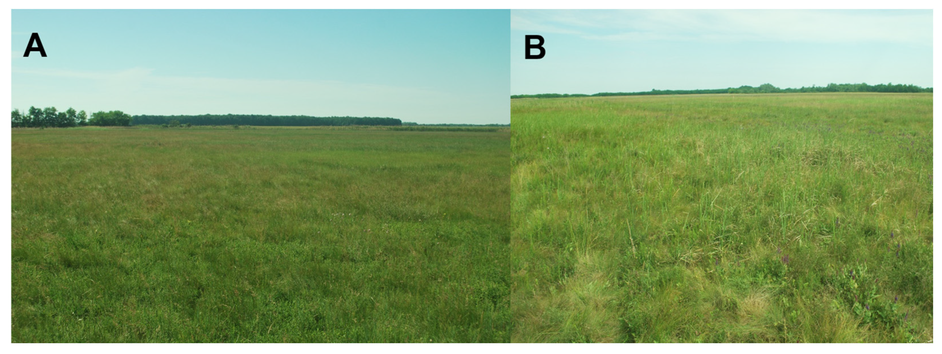
The study area is located in the Great Hungarian Plain, at Tompapuszta (46.360° N, 20.980° E), near the town of Battonya in Hungary (CE Europe) (Figure A1). The strictly protected area (‘Tompapusztai-löszgyep’) is part of the Körös–Maros National Park, and it represents a climatically zonal, well-preserved loess meadow steppe developed on humus-rich chernozem soil formed over a loess substrate. The dominant species of the primary grassland was Festuca valesiaca. Other abundant plant species included several perennial graminoids, such as Poa angustifolia, Alopecurus pratensis, Carex praecox and Elymus hispidus, and perennial forbs, including Teucrium chamaedrys, Galium verum, Fragaria viridis, Thymus pannonicus and Salvia nemorosa [48]. The region is characterized by a warm temperate climate with a sub-Mediterranean influence. The mean annual precipitation ranges from 500 to 550 mm, while the mean annual temperature is between 10 and 11 °C (based on 30 years of meteorological data, 1960–1990). Since 2009, several agricultural fields have been abandoned around the protected area. We chose two secondary grasslands developing on these abandoned fields. These old fields were selected to study spontaneous succession because they were adjacent to the natural (primary) grassland. Both fields were abandoned in 2009. In 2011, two monitoring sites were established in the spontaneously developing old fields as secondary grassland sites (S1, S2), together with two reference monitoring sites as primary grassland sites (P1, P2) in the pristine meadow steppe. The selected sites were open flat areas (without shrubs or trees) with similar elevation (99 m a.s.l.). They were physiognomically homogeneous, without microtopographical or microclimatic differences. Disturbed areas (e.g., old roads) and small depressions were avoided during site selection. Primary and secondary grasslands shared the same species pool, had similar chernozem soil, experienced the same weather and were similarly managed (mowed once a year) during the study period. The dominant species were largely shared between the primary and the secondary grasslands, providing ideal conditions to address our aim of comparing the behavior of the same species (Figure A2).

2.2. Field Sampling

At each monitoring site, one 52 m long permanent belt transect was selected randomly within a homogeneous area. They were sampled annually in late May or early June, during the phenological optima of the communities, for fifteen consecutive years between 2011 and 2025. However, in this study, we present results from the last seven years (from 2019 to 2025), because the three matrix grasses (family Poaceae) of the primary meadow steppe (Festuca valesiaca, Poa angustifolia, Alopecurus pratensis) became the most abundant species in the secondary grasslands only in 2019 (Supplementary Materials S1). The abandoned field was 10 years old at the start of the study in 2019 and 16 years old by its end in 2025. The transects were topologically circular (arranged in rectangular form; see Figure S2.1). The four corners of the rectangular transects were permanently marked. The presence of the species was recorded along transects in 5 cm × 5 cm sampling units. We opted for the use of this sampling method as our previous methodological studies proved that this high-resolution and high-extent sampling design is optimal for the monitoring of spatial variability and heterogeneity in grasslands [36]. Furthermore, the topologically circular arrangement of contiguous microquadrats along the transects enables the application of computerized sampling [36,49] and various types of randomization in null model tests, providing a wide range of analytical tools that were well suited to our research objectives. The distance between the two secondary grassland transects (S1 and S2) was more than 400 m, while the distance between the primary grassland transects (P1 and P2) was more than 350 m. In each sampling campaign, we sampled 4 × 1040 = 4160 microquadrats. This resulted in 62,400 microquadrats over 15 years of monitoring. For the present study, we used a subset, consisting of 29,120 microquadrats (corresponding to the final 7 of the 15 years) of this large database. The time series of the baseline transect data were resampled with computerized sampling for further analyses.

2.3. Data Analysis

The baseline transect data were resampled into regularly arranged 1 m segments, and species abundances were calculated for each segment by summarizing the presence of species within that particular segment. These data were then used to create spatiotemporal maps of species abundances.
The patterns of species presence were rescaled from the 5 cm resolution to coarser spatial scales (to 10 cm and 20 cm resolutions; Figure S2.2) to decrease the potential pseudo-turnovers between years [50]. These rescaled data were used to analyze temporal patterns, i.e., temporal associations and the rates of temporal changes in microquadrats.

2.4. Testing for Significant Spatial Aggregation of Species Using Information Theory Models

The spatial entropy function, Hx, derived from the information theory models of Pál Juhász-Nagy [51,52], was used to calculate the spatial aggregation of species. Hx represents the uncertainty of finding a species in a sampling unit.
  • Hx can be calculated as
    Hx = − px ∗ log px − (1 − px) ∗ log (1 − px)
    where px is the probability of the presence of species x, and (1 − px) is the probability of its absence in the sample (for more details, see Supplementary Materials S3).
Hx is a function of the sampling unit size (Figure S3.1). Therefore, Hx was estimated across a range of scales (at changing sampling unit sizes) from 5 cm × 5 cm to 5 cm × 1875 cm by merging two, three, four, etc., to a total of 375 consecutive microquadrats by subsequent computerized sampling in 48 spatial steps [36,49]. The significance of spatial aggregation was tested against a null model of the complete spatial randomness of species presence along the transect. The randomization was repeated 999 times for each test. Significance was expressed as a probability of the observed Hx under the null model. As Hx varies only between 0 and 1, the spatial pattern of a species can be characterized by the spatial scale (i.e., sampling unit size) at which its Hx reaches the maximum. This is the characteristic maximum scale, S-Hx, of the given species x [52]. More aggregated species have larger values of S-Hx. To compare the spatial aggregation of species with different abundances, we used an index of aggregation, Iaggr:
I a g g r = log S H x ( o b s e r v e d ) log S H x ( r a n d o m )
where S–Hx (observed) is the spatial scale at which the spatial entropy of the field data reaches its maximum, and S–Hx (random) is the spatial scale where the mean spatial entropy function of a null model has its maximum (mean of 999 random patterns generated with the same abundance as in the field data).

2.5. Quantifying Temporal Dependence in Time Series of Species Patterns Using Information Theory Models

We used the Associatum function derived from the information theory models of Pál Juhász-Nagy [51,52,53] to quantify the overall temporal dependence among the spatial patterns of a given plant species across different years. In this study, we used a modified version of the original model. We considered the spatial pattern of each species individually over time and estimated the temporal combinations of presence and absence that appeared in a given permanent microquadrat over the years. Based on this, Temporal Associatum represents the overall spatial dependence among the spatial patterns of a given species across different years, which can be expressed as the difference between two Shannon diversities [54]: the diversity of expected temporal combinations and the diversity of observed temporal combinations.
T e m p o r a l   A s s o c i a t u m   t 1 ,   t 2 , t 3 t n = f = 1 f = z p f e x p × log p f e x p f = 1 f = z p f o b s × log p f o b s
where pf is the probability of a particular temporal combination f, and f ranges from 1 to z = 2n, where n is the number of years in the analysis.
As shown in Figure S4, Temporal Associatum is a scale-dependent variable. Therefore, Temporal Associatum was estimated across a range of scales (at changing sampling unit sizes) from 5 cm × 10 cm to 5 cm × 990 cm by merging two, three, four, etc., to a total of 198 consecutive microquadrats by subsequent computerized sampling in 13 spatial steps [36,49]. The significance of associations was tested against a null model of the complete spatial randomness of species presence along transects. The randomization was repeated 999 times for each test. Significance was expressed as a probability of the observed Temporal Associatum under the null model (for more details, see Supplementary Materials S4).
The rates of the fine-scale dynamics within a certain species were calculated via the following formulas:
R a t e   o f   g a i n = n u m b e r   o f   m i c r o q u a d r a t s   t h a t   t r a n s f o r m e d   i n t o   p r e s e n c e   i n   y e a r   t   f r o m   p r e v i o u s   y e a r   a b s e n c e   t o t a l   n u m b e r   o f   p r e s e n c e s   i n   y e a r   t
R a t e   o f   l o s s = n u m b e r   o f   m i c r o q u a d r a t s   t h a t   t r a n s f o r m e d   i n t o   a b s e n c e   i n   y e a r   t   f r o m   p r e v i o u s   y e a r   p r e s e n c e   t o t a l   n u m b e r   o f   p r e s e n c e s   i n   t h e   p r e v i o u s   ( t 1 )   y e a r
The JNP-model 2.0 software [55] was used to perform the computerized sampling and the analyses of spatial aggregations and temporal associations, including the randomization tests. Since the spatial aggregation data did not follow a normal distribution, we used a non-parametric Friedman test to detect significant differences between the spatial aggregation indices of different plant species within the same vegetation stand, as well as to detect differences between the spatial aggregation indices of the same plant species across different vegetation stands. We consider yearly measures as repeated observations. As a post hoc test, we used the Wilcoxon signed-rank test with the Bonferroni–Holm correction due to the multiple comparisons. Adjusted p-values are indicated, and p < 0.05 is considered statistically significant. The temporal patterns of the spatial variability in subordinated species richness were compared in a similar way. In the comparison of the distribution of fine-scale local richness (multiplets) and of local species combinations of matrix species in the primary and secondary grasslands, we used chi-squared tests. The pooled datasets of gains and losses (i.e., the rate of changes) of the three matrix species between the primary and secondary grassland sites were compared via the Mann–Whitney U test.
All statistical analyses were conducted using the Past v5.2.1 software package [56].

3. Results

Visual inspection revealed high variability and distinct patterns (patchiness) between the primary and secondary grasslands in both space and time (Figure 1, Supplementary Figure S5).
Festuca valesiaca had similar abundances and patterns in the primary sites and in one secondary grassland site (S2). In the other secondary grassland site (S1), the species showed an increasing trend but became equally abundant as in the other sites during the final three years (Figure S5.1). Poa angustifolia was the second most abundant species in the primary grassland sites and in the S1 secondary site. Its abundance decreased in 2023 in all sites due to a serious drought in 2022, but it later started to recover. The abundance of Alopecurus pratensis slightly decreased in the primary grassland sites, especially after the drought in 2022, while it had an increasing trend in the secondary grassland sites over the same period.
All species showed significant deviations from the spatially randomized null models in at least some years (p < 0.01, Supplementary Materials S6). The degree of aggregation was species-specific and it varied both among sites and over time (Supplementary Materials S7).
In the secondary grassland sites, Poa angustifolia showed very strong but temporally decreasing spatial aggregation in this period (Figure 2) (median Iaggr = 1.65). The aggregation of Alopecurus pratensis was also strong (median Iaggr = 1.39) but slightly lower, and it increased over time. The aggregation index of Festuca valesiaca decreased and converged to one, i.e., its fine-scale spatial variability did not deviate from the random null model. The spatial pattern of Festuca valesiaca was random or close to random, even in the primary grassland sites. Here, Alopecurus pratensis showed the highest degree of aggregation, which remained relatively stable over the study period (median Iaggr = 1.18). In the primary grassland sites, the aggregation index of Poa angustifolia did not deviate from the null model in the early period of our study, but then it started to increase (median Iaggr = 1.08). Evaluating the overall temporal patterns, we can conclude that the spatial aggregation of Alopecurus pratensis and Poa angustifolia showed significantly higher values in secondary grassland sites than in primary grassland sites across all years (Friedman test, p < 0.001; Supplementary Table S7), while Festuca valesiaca showed lower aggregation values in all years, with no difference between secondary and primary grasslands (Friedman test, p = 0.542; Supplementary Table S7).
Our study demonstrated strong associations among the spatial patterns of each species across different years (Supplementary Materials S8). A Wilcoxon signed-rank test was conducted to compare the maximum values of temporal association of the three matrix species between the primary and secondary grasslands. The results showed a significant difference (W = 0, p = 0.0022), indicating higher temporal dependence in the secondary grassland sites. The degree of temporal dependence was higher in the secondary grassland sites, especially in the case of Poa angustifolia and Alopecurus pratensis. Associations were scale-dependent, and they appeared at coarser scales in secondary grassland sites (Figure 3).
Comparing the presence of a given species in specific microquadrats between subsequent years revealed high temporal variability. Alopecurus pratensis displayed the highest dynamics in the primary grassland sites (Figure 4). When estimated at a 10 cm resolution, the average rate of losses of Alopecurus pratensis was between 0.59 and 0.64, i.e., about 59–64% of presences became absences from one year to another; in addition, in the following year, a similar proportion of new presences appeared.
Alopecurus pratensis and Poa angustifolia were more dynamic in the primary grassland sites, while the mean rates of change was generally lower in the case of Festuca valesiaca, with similar values in the primary and secondary grasslands. When estimated at a 10 cm resolution, ca. 20–30% of Festuca valesiaca presences were lost or gained between subsequent years. Repeating these estimations at a 20 cm resolution, the actual rate of change decreased slightly, but the overall patterns remained similar. In the primary grassland sites, Alopecurus pratensis was the most dynamic matrix species (with 46–59% mean gains and losses between years), while Festuca valesiaca was the most persistent. The overall rates of both gains and losses of all three matrix species were compared using the Mann–Whitney U test between the primary and secondary stands. We found a significant difference between them, but only in the case of the 10 cm resolution data, where the primary stands showed higher rate of change by ca. 49% (U = 36, p = 0.04) (Supplementary Materials S9).
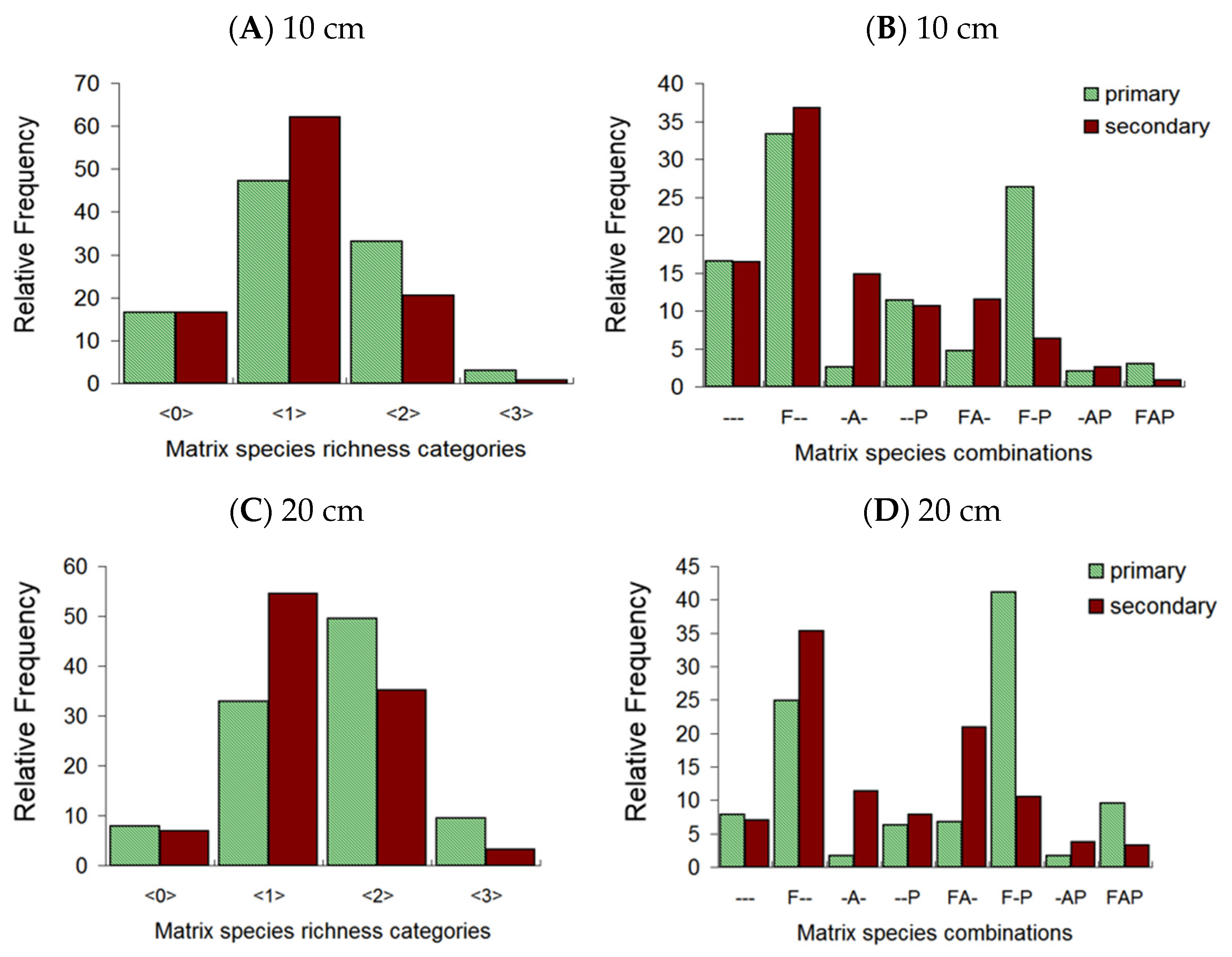
The spatial patterns of the different species overlapped in the vegetation matrix. When analyzed at a 10 cm resolution, 47% of the microquadrats consisted of only one matrix species in the primary grassland sites, while 36% of the microquadrats had two or all three species (Figure 5).
In contrast, the frequency of the single-species microquadrats was larger in the secondary grassland sites (62%), and only 21% of microquadrats had two or three species. Further analysis of the collective patterns of matrix species revealed that the most abundant species combination was Festuca valesiaca occurring alone, at 33% in the primary and 37% in the secondary grasslands, respectively. The second most frequent combination was the two-species combination of Festuca valesiaca–Poa angustifolia in the primary grassland (26%) and the Alopecurus pratensis single-species combination in the secondary grassland (15%). At a 20 cm resolution, the analysis showed that the distribution of species richness categories followed a similar shape. The overall pattern of species combinations changed slightly: in the primary grasslands, the Festuca valesiaca–Poa angustifolia two-species combination became the most frequent (41%), while, in the secondary grasslands, the Festuca valesiaca single-species combination remained the most frequent (35%). We performed an χ2 test to compare the distributions of species richness categories and that of matrix species combinations among primary and secondary sites. We found significant differences between the distributions in both scales (p < 0.05 in the case of species richness categories and p < 0.001 in the case of species combinations). Primary grassland sites tended to bear more quadrats with higher species numbers (two or three) and fewer quadrats had only one species. For further details, see Supplementary Figure S10. These results provide evidence of the variability in microhabitats in primary and secondary grasslands.
The relative spatial variability (CV%) of local species richness was consistently larger in the secondary grassland sites throughout the study period (2019–2025), and this relationship persisted across all spatial scales (at 5 cm, 10 cm and 20 cm resolutions; Friedman test, p < 0.001; Supplementary Materials S11). Temporal patterns were remarkably similar between replicates of both grassland types (Figure 6). The relative spatial variability in local matrix species richness changed little in the primary grasslands (only with a very slight decrease), while it showed an increasing trend in the secondary grassland sites.

4. Discussion

Our study revealed high fine-scale variability and significant spatiotemporal dependences (patchiness) in all studied grasslands. However, secondary grasslands exhibited a stronger dependence in both space and time. Each matrix species displayed distinct fine-scale dynamics and different patterns of co-occurrence in primary and secondary grasslands. Moreover, the spatial variation in subordinated species richness was consistently larger in secondary grasslands.

4.1. Spatial Patterns of Matrix Species

We used the spatial entropy, Hx—an information theory measure—to detect spatial dependences within dominant species. Unlike alternative methods [57,58], with the use of Hx, we did not intend to detect the mean patch size within a species’ spatial pattern. Rather, Hx quantifies the uncertainty of finding a certain species within a sampling unit of a specified size. From an ecological point of view, the used spatial entropy reflects the uncertainty (i.e., the inverse of the probability) that a colonizing subordinate individual will encounter a particular dominant species within an ecologically relevant neighborhood [59]. The size of this ecological neighborhood corresponds to the size of the sampling unit used to estimate Hx. Thus, this interpretation of Hx provides a useful link to the dynamics of the community. Under ideal conditions, species are expected to interact in proportion to their relative abundances. Hx calculated from randomized reference patterns reflects the associated probability (cf. mean field approximation [60]). Species with aggregated spatial patterns will interact with lower probabilities, resulting in community dynamics that deviate from those predicted by mean field approximation. The stronger the spatial aggregation, the larger the differences between the observed dynamics and the idealized dynamics based on mean field approximation [60].
In this context, our study demonstrated that spatial constraints were present in all vegetation matrices at the studied sites. The magnitude of these constraints varied among matrix species and was generally greater in secondary grasslands. These results support our first hypothesis (H1) that matrix species exhibit more aggregated spatial patterns in secondary grasslands.
Species with low abundances typically form distinct small patches, which expand and coalesce as the species abundances grow and exceed a certain threshold [23,24]. In our study, Festuca valesiaca appeared to reach this threshold, exhibiting a spatial distribution that was random or nearly random across all sites. In contrast, no consistent relationship between abundance and spatial aggregation was observed for Alopecurus pratensis and Poa angustifolia. Our study sites experienced an extreme climatic event during the summer of 2022, characterized by severe drought and heatwaves (Supplementary Materials S12) [61]. Festuca valesiaca and Poa angustifolia responded to this climatic extreme with reduced abundances and slightly increased spatial aggregation in primary grasslands. In secondary grasslands, both species exhibited similar but weaker declines in abundance, without clear changes in their spatial patterns.
Studies examining spatial patterns in grasslands have primarily focused on the effects of grazing intensity or land abandonment [33,62]. Spatial heterogeneity tends to increase following the cessation of grassland management [63]. Grazing, in turn, can either enhance or reduce patchiness, depending on how vegetation patterns interact with the spatial distribution of grazing pressure [64]. Moderate to high grazing intensities tend to increase patchiness, whereas very heavy grazing leads to more homogeneous vegetation patterns dominated by weeds [32]. Heterogeneous patchworks exhibiting varying degrees of spatial dependence among species have also been reported in secondary grasslands developing on abandoned agricultural fields [42,62,65]. However, drawing general conclusions remains challenging, as many of these studies rely on space-for-time substitution, comparing secondary grasslands with differing histories, land-use legacies, and landscape contexts.

4.2. Temporal Dependence and Fine-Scale Dynamics

Consistent with our second hypothesis (H2), we found significant temporal associations in the time series of the spatial patterns of individual matrix species, with stronger relationships observed in the secondary grasslands. This indicates that the overall spatial configuration of a species’ distribution changed gradually and remained relatively stable across the years. In a similar study, Herben et al. [66] reported considerable variation in temporal autocorrelations among species in two mountain grasslands. The strength of these temporal dependencies was associated with species’ mobility traits. In line with our findings, they observed strong temporal autocorrelations in the case of the dominant grass species as well.
One might expect a relationship between spatial and temporal dependence whereby species with a weak spatial structure would also show weak temporal stability. Accordingly, we expected low temporal dependence in species with nearly random spatial distributions. On the contrary, both Festuca valesiaca and Poa angustifolia exhibited significant temporal associations in the primary grasslands, despite their spatial distributions being close to random. In contrast, Alopecurus pratensis showed strong spatial aggregation, while displaying strong temporal dependence. Overall, species with the most pronounced spatial patchiness tended to exhibit the strongest temporal dependence. During our seven-year study, the secondary grasslands changed from 10 to 16 years old. The spatiotemporal patterns of species demonstrated clearly that the centroids of their patches remained near the locality of their first establishment. Priority effects, limited dispersal [26,43] and their dynamic clonal morphological traits [27] explain these spatial dynamics.
In contrast to our hypothesis (H3), the rates of fine-scale temporal changes (i.e., the percentage of presences gained or lost between years) were lower in secondary stands in the case of Alopecurus pratensis. Poa angustifolia had lower rates only in one of the secondary grasslands. In the case of Festuca valesiaca, the rates of fine-scale loss and gain of presence were similar in all grasslands. The high between-year turnover of individual presences does not imply the absence of temporal associations in species patterns. The rate of turnover varied between 20% and 70%, meaning that the remaining 80–30% of presences persisted. This persistent portion of presences maintained the coarse-scale shape of the spatial patterns over time, generating temporal associations.

4.3. Co-Occurrence Patterns of Matrix Species and Responses of Subordinates

Our findings revealed that matrix species created microhabitats through various fine-scale combinations. At the ecologically relevant scale of species interactions (at a 20 cm resolution), most microhabitats in secondary grasslands were formed by a single matrix species. In contrast, in primary grasslands, the most abundant microhabitats appeared with two or three matrix species. When combined with the observed differences in the scales and magnitudes of spatial and temporal dependences, these patterns reveal contrasting ecological dynamics between primary and secondary grasslands (Table 1).
In secondary grasslands, matrix species form coarse-grained mosaics composed mainly of mono-specific, temporally stable patches. In contrast, primary grasslands are more dynamic and complex, characterized by fine-grain multispecies patches. These differences in the patterns of matrix species might influence the occurrence and dynamics of subordinate species. Previous studies reported increasing structure and increasing selection against inappropriate species combinations in succession [43,55] and stronger assembly rules in mature communities [47,55]. Based on this evidence, we expected stochastic patterns in recovering secondary grasslands and stronger pattern selection in primary grasslands. We hypothesized [H4] that stronger pattern selection would result in higher fine-scale spatial variability in subordinate species richness in the primary grasslands. However, contrary to our hypothesis, the spatial variability in subordinate species richness was higher in the secondary grasslands. The stochastic patterns predicted in our hypothesis may be characteristic of earlier successional stages. Our results suggest that microhabitats in secondary grasslands formed by larger and temporally more persistent patches of dominant species likely exerted stronger and spatially more distinct selection among subordinates. These processes might lead to greater microhabitat heterogeneity, which explains the higher spatial variation in subordinate species richness observed in secondary grasslands. Several other studies have documented strong spatial filtering by dominant species in mid-successional communities (in vegetation types comparable to our secondary grasslands) [61,62,67].

4.4. Limitations and Perspectives

Our aim was to identify consistent differences between primary and secondary grasslands. To minimize confounding factors, we focused on a specific type of secondary grassland: mid-successional old fields undergoing natural regeneration following agricultural abandonment, located adjacent to a pristine, undisturbed grassland. The nearby primary grassland served as a propagule source for the recovering old field, which led to a similar species pool and the presence of the same matrix species across all sites. In addition, all study sites shared comparable environmental conditions.
We analyzed only two replicates of each grassland type. Therefore, our results (Table 1) are limited and preliminary. However, to our knowledge, no similar long-term study is available where the fine-scale spatiotemporal organization of primary and secondary grasslands has been compared. All characteristics studied in this work were scale-dependent. To assess variability and spatiotemporal patterns accurately, we needed high-resolution, spatially explicit data recorded in contiguous microquadrats. To represent multiple-scale spatial variation, the size of the sample had to be large. Therefore, we used long permanent transects for monitoring. This sampling design provides data with a high spatial resolution and high spatial extent, and it has successfully been applied in various grassland types [36]. To detect temporal variability and temporal associations in a representative way, we had to repeat our sampling over several years. These criteria resulted in laborious sampling protocols that constrained the number of sites that we were able to study. Despite the limited number of replicates, our study contributes to filling an important gap in current knowledge. We are only aware of three similar data sets in grasslands, where high-resolution spatial mapping was repeated in the framework of a continuous, long-term study [37,68,69].
Comparing primary and secondary ecosystems is both relevant and timely. As human impacts continue to increase globally, larger portions of the Earth’s landscape are becoming secondary and will exist in various states of regeneration following disturbances [70]. Ecological theory indicates fundamental differences between young, immature and old-growth, mature ecosystems [71]. To test this theory and facilitate the regeneration and functional convergence of young ecosystems toward mature states, more long-term comparative studies are needed.

5. Conclusions

This study presents a unique case in which the same matrix species were monitored in adjacent primary and secondary grassland sites. All grasslands exhibited dynamic spatial organization with high fine-scale variability. Our results showed that matrix species self-organize into dynamic patchworks, where patches emerge, grow or decrease in size and interact with neighbors. While some patches persisted over time, others disappeared. In addition, the spatial patterns and dynamics of each species differed between grassland types. These findings provide evidence of characteristic differences between primary and secondary grasslands. The local variability in these processes contributed to the overall diversity of the vegetation matrix, creating diverse microhabitats for subordinate species. With this work, we would like to emphasize that monitoring the fine-scale organization of the vegetation matrix offers valuable information for grassland conservation and restoration efforts.

Supplementary Materials

The following supporting information can be downloaded at: https://www.mdpi.com/article/10.3390/land14091736/s1. Supplementary S1. Selection of study species. Supplementary S2. Sampling design and rescaling the baseline data. Supplementary S3. Quantifying spatial aggregation of species using information theory models. Supplementary S4. Quantifying the temporal dependence in time series of single-species spatial patterns using information theory models. Supplementary S5. Abundance patterns and rank relations of study species. Supplementary S6. Detailed results of the spatial entropy analyses quantifying the degree of spatial aggregation of species using information theory models. Supplementary S7. Comparing the temporal patterns of aggregation of different species. Supplementary S8. Detailed results of the Temporal Associatum analyses quantifying the temporal dependence in time series of single-species spatial patterns using information theory models. Supplementary S9. Comparison of the rates of change in primary and secondary grasslands. Supplementary S10. Comparison of the distribution of multiplets and species combinations in primary and secondary grasslands. Supplementary S11. Comparing temporal patterns of the variability of subordinate species richness between primary and secondary grasslands. Supplementary S12. Precipitation and temperature during the sampling period.

Author Contributions

Conceptualization, S.B., S.C. and A.I.C.; methodology, S.B.; software, S.B. and S.C.; validation, A.I.C. and S.B.; formal analysis, S.C. and S.B.; investigation, D.P., J.H., Z.Z., Z.E.G., S.C., G.S. and A.I.C.; data curation, A.I.C.; writing—original draft preparation, S.B. and S.C.; writing—review and editing, all authors; visualization, S.B.; supervision, A.I.C.; project administration, A.I.C. All authors have read and agreed to the published version of the manuscript.

Funding

This research was funded by the FLAGSHIP RESEARCH GROUPS PROGRAMME 2024 of the Hungarian University of Agriculture and Life Sciences.

Data Availability Statement

Data are available from A.I.C. upon reasonable request.

Acknowledgments

We would like to thank András János Csathó, Csaba Molnár, Melinda Juhász, Róbert Kun, Zsuzsanna Sutyinszki, Szilárd Szentes, Klára Virágh and Cecília Komoly for their help in data collection. We thank the Körös–Maros National Park Directorate for their support.

Conflicts of Interest

The authors declare no conflicts of interest.

Abbreviations

The following abbreviations are used in this manuscript:
HxSpatial entropy function
IaggrAggregation index

Appendix A

Figure A1. Location of the study area in Hungary and in Europe. Blue color shows rivers and lakes. Green circle marks the location of the study area near the town of Battonya.
Land 14 01736 g0a1
Figure A2. Study grasslands near Battonya in Hungary. (A) Primary grassland in 2025. (B) Secondary grassland (16-year-old spontaneously recovering abandoned agricultural field) in 2025 (photo from S. Bartha).
Land 14 01736 g0a2

References

  1. Whittaker, R.H. Dominance and diversity in land plant communities. Science 1965, 147, 250–260. [Google Scholar] [CrossRef]
  2. Grime, J.P. Benefits of plant diversity to ecosystems: Immediate, filter and founder effects. J. Ecol. 1998, 86, 902–910. [Google Scholar] [CrossRef]
  3. Avolio, M.L.; Forrestel, E.J.; Chang, C.C.; La Pierre, K.J.; Burghardt, K.T.; Smith, M.D. Demystifying dominant species. New Phytol. 2019, 223, 1106–1126. [Google Scholar] [CrossRef]
  4. Smith, M.D.; Knapp, A.K. Dominant species maintain ecosystem function with non-random species loss. Ecol. Lett. 2003, 6, 509–517. [Google Scholar] [CrossRef]
  5. Wilsey, B.J. Productivity and Subordinate Species Response to Dominant Grass Species and Seed Source during Restoration. Restor. Ecol. 2010, 18, 628–637. [Google Scholar] [CrossRef]
  6. Kikvidze, Z.; Brooker, R.W.; Butterfield, B.J.; Callaway, R.M.; Cavieres, L.A.; Cook, B.J.; Lortie, C.J.; Michalet, R.; Pugnaire, F.I.; Xiao, S.; et al. The effects of foundation species on community assembly: A global study on alpine cushion plant communities. Ecology 2015, 96, 2064–2069. [Google Scholar] [CrossRef] [PubMed]
  7. Akatov, V.V.; Akatova, T.V.; Eskina, T.G.; Sazonets, N.M.; Chefranov, S.G. Dominants in plant communities: The nature of impact on biomass determines the thresholds of impact on local species richness. Biol. Bull. Rev. 2025, 15, 12–23. [Google Scholar] [CrossRef]
  8. Zhang, P.; Seabloom, E.W.; Foo, J.; MacDougall, A.S.; Harpole, W.S.; Adler, P.B.; Hautier, Y.; Eisenhauer, N.; Spohn, M.; Bakker, J.D.; et al. Dominant species predict plant richness and biomass in global grasslands. Nat. Ecol. Evol. 2025, 9, 924–936. [Google Scholar] [CrossRef] [PubMed]
  9. Jones, S.K.; Ripplinger, J.; Collins, S.L. Species reordering, not changes in richness, drives long-term dynamics in grassland communities. Ecol. Lett. 2017, 20, 1556–1565. [Google Scholar] [CrossRef]
  10. Hou, G.; Shi, P.; Zhou, T.; Sun, J.; Zong, N.; Song, M.; Zhang, X. Dominant species play a leading role in shaping community stability in the northern Tibetan grasslands. J. Plant Ecol. 2023, 16, 110. [Google Scholar] [CrossRef]
  11. Adler, P.B.; HilleRisLambert, J.; Kyriakidis, P.C.; Guan, Q.; Levine, J.M. Climate variability has a stabilizing effect on the coexistence of prairie grasses. Proc. Natl. Acad. Sci. USA 2006, 103, 12793–12798. [Google Scholar] [CrossRef]
  12. Falinski, J.B. Vegetation Dynamics in Temperate Lowland Primeval Forests. Ecological Studies in Białowieza Forest; Springer: Dordrecht, The Netherlands, 1986; p. 537. [Google Scholar] [CrossRef]
  13. Bobiec, A. The mosaic diversity of field layer vegetation in the natural and exploited forests of Bialowieza. Plant Ecol. 1998, 136, 175–187. [Google Scholar] [CrossRef]
  14. Brearley, F.Q.; Prajadinata, S.; Kidd, P.S.; Proctor, J.; Suriantata. Structure and floristics of an old secondary rain forest in Central Kalimantan, Indonesia, and a comparison with adjacent primary forest. For. Ecol. Manag. 2004, 195, 385–397. [Google Scholar] [CrossRef]
  15. Korepin, A.A.; Kapitsa, E.A.; Shorohov, A.A. Half-Century Dynamics of Primary and Secondary Tree Stands in the Veps Forest Natural Reserve. Contemp. Probl. Ecol. 2024, 17, 996–1008. [Google Scholar] [CrossRef]
  16. Ehbrecht, M.; Seidel, D.; Annighöfer, P.; Kreft, H.; Köhler, M.; Zemp, D.C.; Puettmann, K.; Nilus, R.; Babweteera, F.; Willim, K.; et al. Global patterns and climatic controls of forest structural complexity. Nat. Commun. 2021, 12, 519. [Google Scholar] [CrossRef]
  17. Wang, T.; Dong, L.; Liu, Z. Stand structure is more important for forest productivity stability than tree, understory plant and soil biota species diversity. Front. For. Glob. Change 2024, 7, 1354508. [Google Scholar] [CrossRef]
  18. Illyés, E.; Chytrý, M.; Botta-Dukát, Z.; Jandt, U.; Škodová, I.; Janišová, M.; Willner, W.; Hájek, O. Semi-dry grasslands along a climatic gradient across Central Europe: Vegetation classification with validation. J. Veg. Sci. 2007, 18, 835–846. [Google Scholar] [CrossRef]
  19. Velev, N.; Apostolova, I. Successional changes of Nardus stricta communities in the Central Balkan Range (Bulgaria). Phytol. Balc. 2008, 14, 75–84. [Google Scholar]
  20. Dengler, J.; Janisová, M.; Török, P.; Wellstein, C. Biodiversity of Palaearctic grasslands: A synthesis. Agric. Ecosyst. Environ. 2015, 182, 1–14. [Google Scholar] [CrossRef]
  21. Biurrun, I.; Pielech, R.; Dembicz, I.; Gillet, F.; Kozub, Ł.; Marcenò, C.; Reitalu, T.; Van Meerbeek, K.; Guarino, R.; Chytrý, M.; et al. Benchmarking plant diversity of Palaearctic grasslands and other open habitats. J. Veg. Sci. 2021, 32, e13050. [Google Scholar] [CrossRef]
  22. Prach, K.; Török, P.; Bakker, J.D. Temperate grasslands. In Routledge Handbook of Ecological and Environmental Restoration; Taylor & Francis: Abingdon, UK, 2017; pp. 126–141. [Google Scholar]
  23. Greig-Smith, P. Pattern in vegetation. J. Ecol. 1979, 67, 755–779. [Google Scholar] [CrossRef]
  24. Kershaw, K.A. Pattern in vegetation and its causality. Ecology 1963, 44, 377–388. [Google Scholar] [CrossRef]
  25. Gibson, D.J. The relationship of sheep grazing and soil heterogeneity to plant spatial patterns in dune grassland. J. Ecol. 1988, 76, 233–252. [Google Scholar] [CrossRef]
  26. Seabloom, E.W.; Bjørnstad, O.N.; Bolker, B.M.; Reichman, O.J. Spatial signature of environmental heterogeneity, dispersal, and competition in successional grasslands. Ecol. Monogr. 2005, 75, 199–214. [Google Scholar] [CrossRef]
  27. Benot, M.L.; Bittebiere, A.K.; Ernoult, A.; Clément, B.; Mony, C. Fine-scale spatial patterns in grassland communities depend on species clonal dispersal ability and interactions with neighbours. J. Ecol. 2013, 101, 626–636. [Google Scholar] [CrossRef]
  28. De Benedictis, L.L.M.; Chelli, S.; Canullo, R.; Campetella, G. Measuring them all: Individual-based functional spatial patterns in mountain grasslands. J. Veg. Sci. 2025, 36, e70029. [Google Scholar] [CrossRef]
  29. Chesson, P.; Neuhauser, C. Intraspecific aggregation and species coexistence. Trends Ecol. Evol. 2002, 17, 210–211. [Google Scholar] [CrossRef]
  30. Bolker, B.M.; Pacala, S.W.; Neuhauser, C. Spatial dynamics in model plant communities: What do we really know? Am. Nat. 2003, 162, 135–148. [Google Scholar] [CrossRef]
  31. Wiegand, T.; Wang, X.; Anderson-Teixeira, K.J.; Bourg, N.A.; Cao, M.; Ci, X.; Davies, S.J.; Hao, Z.; Howe, R.W.; Kress, W.J.; et al. Consequences of spatial patterns for coexistence in species-rich plant communities. Nat. Ecol. Evol. 2021, 5, 965–973. [Google Scholar] [CrossRef] [PubMed]
  32. Bartha, S. Composition, differentiation and dynamics in the forest steppe biome. In Slope Steppes, Loess Steppes and Forest Steppe Meadows in Hungary; Illyés, E., Bölöni, J., Eds.; MTA ÖBKI: Budapest, Hungary, 2007; pp. 194–210. [Google Scholar]
  33. Virágh, K.; Horváth, A.; Bartha, S.; Somodi, I. A multiscale methodological approach for monitoring the effectiveness of grassland management. Community Ecol. 2008, 9, 237–246. [Google Scholar] [CrossRef]
  34. Kéfi, S.; Guttal, V.; Brock, W.A.; Carpenter, S.R.; Ellison, A.M.; Livina, V.N.; Seekell, D.A.; Scheffer, M.; van Nes, E.H.; Dakos, V.; et al. Early warning signals of ecological transitions: Methods for spatial patterns. PLoS ONE 2014, 9, e92097. [Google Scholar] [CrossRef]
  35. Fehmi, J.S.; Bartolome, J.W. A grid-based method for sampling and analysing spatially ambiguous plants. J. Veg. Sci. 2001, 12, 467–472. [Google Scholar] [CrossRef]
  36. Bartha, S.; Campatella, G.; Canullo, R.; Bódis, J.; Mucina, L. On the importance of fine-scale spatial complexity in vegetation restoration. Int. J. Ecol. Environ. Sci. 2004, 30, 101–116. [Google Scholar]
  37. Chen, X.; Li, B.; Collins, S.L. Multiscale monitoring of a multispecies case study: Two grass species at Sevilleta. Plant Ecol. 2005, 179, 149–154. [Google Scholar] [CrossRef]
  38. Collins, S.L.; Xia, Y. Long-term dynamics and hotspots of change in a desert grassland plant community. Am. Nat. 2015, 185, E30–E43. [Google Scholar] [CrossRef] [PubMed]
  39. Dobson, A.P.; Bradshaw, A.D.; Baker, A.J.M. Hopes for the future: Restoration Ecology and Conservation Biology. Science 1997, 277, 515–522. [Google Scholar] [CrossRef]
  40. Hölzel, N.; Haub, C.; Ingelfinger, M.P.; Otte, A.; Pilipenko, V.N. The return of the steppe: Largescale restoration of degraded land in southern Russia during the post-Soviet era. J. Nat. Conserv. 2002, 10, 75–85. [Google Scholar] [CrossRef]
  41. Török, P.; Brudvig, L.A.; Kollmann, J.; Price, J.N.; Tóthmérész, B. The present and future of grassland restoration. Restor. Ecol. 2021, 29, e13378. [Google Scholar] [CrossRef]
  42. Sun, C.; Chai, Z.; Liu, G.; Xue, S. Changes in species diversity patterns and spatial heterogeneity during the secondary succession of grassland vegetation on the loess plateau, China. Front. Plant Sci. 2017, 8, 1465. [Google Scholar] [CrossRef]
  43. Zaplata, M.K.; Winter, S.; Fischer, A.; Kollmann, J.; Ulrich, W. Species-driven phases and increasing structure in early-successional plant communities. Am. Nat. 2013, 181, E17–E27. [Google Scholar] [CrossRef]
  44. Fukami, T. Historical contingency in community assembly: Integrating Niches, Species Pools, and Priority Effects. Annu. Rev. Ecol. Evol. Syst. 2015, 46, 1–23. [Google Scholar] [CrossRef]
  45. Myster, R.W.; Pickett, S.T.A. A comparison of rate of succession over 18 years in 10 contrasting old fields. Ecology 1994, 75, 387–392. [Google Scholar] [CrossRef]
  46. Anderson, K.J. Temporal patterns in rates of community change during succession. Am. Nat. 2007, 169, 780–793. [Google Scholar] [CrossRef]
  47. Wilson, J.B. Assembly rules in plant communities. In Ecological Assembly Rules: Perspectives, Advances, Retreats; Weiher, E., Keddy, P., Eds.; Cambridge University Press: Cambridge, UK, 1999; pp. 130–164. [Google Scholar] [CrossRef]
  48. Csathó, A.J.; Csathó, A.I. The floralist of the Külső-gulya meadow of Battonya-Tompapuszta (SE Hungary). Crisicum 2009, 5, 51–70. [Google Scholar]
  49. Podani, J. Analysis of mapped and simulated vegetation patterns by means of computerized sampling techniques. Acta Bot. Hung. 1984, 30, 403–425. [Google Scholar]
  50. Nilsson, I.N.; Nilsson, S.G. Experimental estimates of census efficiency and pseudoturnover on islands: Error trend and between-observer variation when recording vascular plants. J. Ecol. 1985, 73, 65–70. [Google Scholar] [CrossRef]
  51. Juhász-Nagy, P.; Podani, J. Information theory methods for the study of spatial processes and succession. Vegetatio 1983, 51, 129–140. [Google Scholar] [CrossRef]
  52. Juhász-Nagy, P. Spatial dependence of plant populations. Part 2. A family of new models. Acta Bot. Acad. Sci. Hung. 1984, 30, 363–402. [Google Scholar]
  53. Tsakalos, J.L.; Chelli, S.; Campetella, G.; Canullo, R.; Simonetti, E.; Bartha, S. Comspat: An R package to analyze within-community spatial organization using species combinations. Ecography 2022, 7, e06216. [Google Scholar] [CrossRef]
  54. Shannon, C.E. A mathematical theory of communication. Bell Syst. Tech. J. 1948, 27, 379–423. [Google Scholar] [CrossRef]
  55. Bartha, S.; Czárán, T.; Podani, J. Exploring plant community dynamics in abstract coenostate spaces. Abstr. Bot. 1998, 22, 49–66. [Google Scholar]
  56. Hammer, Ø.; Harper, D.A.T.; Ryan, P.D. PAST: Paleontological statistics software package for education and data analysis. Palaeontol. Electron. 2001, 4, 9. [Google Scholar]
  57. Greig-Smith, P. Quantitative Plant Ecology, 3rd ed.; Blackwell Sci. Pub.: London, UK, 1983; 359p. [Google Scholar]
  58. Dale, M.R.T.; Fortin, M.J. (Eds.) Spatial Analysis: A Guide for Ecologists; Cambridge Univ. Press: New York, NY, USA, 2005; 365p. [Google Scholar]
  59. Addicott, J.F.; Aho, J.M.; Antolin, M.F.; Padilla, D.K.; Richardson, J.S.; Soluk, D.A. Ecological neighborhoods: Scaling environmental patterns. Oikos 1987, 49, 340–346. [Google Scholar] [CrossRef]
  60. Czárán, T. Spatiotemporal Models of Population and Community Dynamics; Chapman & Hall: London, UK, 1998; 284p. [Google Scholar]
  61. Bevacqua, E.; Rakovec, O.; Schumacher, D.L.; Kumar, R.; Thober, S.; Samaniego, L.; Seneviratne, S.I.; Zscheischler, J. Direct and lagged climate change effects intensified the 2022 European drought. Nat. Geosci. 2024, 17, 1100–1107. [Google Scholar] [CrossRef]
  62. Szentes, S.; Sutyinszki, Z.; Szabó, G.; Zimmermann, Z.; Házi, J.; Wichmann, B.; Hufnágel, L.; Penksza, K.; Bartha, S. Grazed pannonian grassland beta-diversity changes due to C4 yellow bluestem. Cent. Eur. J. Biol. 2012, 7, 1055–1065. [Google Scholar] [CrossRef]
  63. Adler, P.B.; Lauenroth, W.K. Livestock exclusion increases the spatial heterogeneity of vegetation in Colorado shortgrass steppe. Appl. Veg. Sci. 2000, 3, 213–222. [Google Scholar] [CrossRef]
  64. Adler, P.B.; Raff, D.A.; Lauenroth, W.K. The effect of grazing on the spatial heterogeneity of vegetation. Oecologia 2001, 128, 465–479. [Google Scholar] [CrossRef] [PubMed]
  65. Lepš, J.; Burianek, V. Interspecific associations in old field succession. In Spatial Processes in Plant Communities; Krahulec, F., Agnew, A.D.Q., Agnew, S., Willems, J.H., Eds.; SPB Publ: The Hague, The Netherlands, 1990; pp. 13–22. [Google Scholar]
  66. Herben, T.; During, H.J.; Krahulec, F. Spatiotemporal dynamics in mountain grasslands: Species autocorrelations in space and time. In Species Coexistence in Temperate Grasslands; Krahulec, F., Goldberg, D.E., Willems, J.H., Eds.; Opulus Press: Uppsala, Sweden, 1995; pp. 79–90. [Google Scholar]
  67. MacCain, K.N.S.; Baer, S.G.; Blair, J.M.; Wilson, G.W.T. Dominant grasses suppress local diversity in restored tallgrass prairie. Restor. Ecol. 2010, 18, 40–49. [Google Scholar] [CrossRef]
  68. Albertson, F.W.; Tomanek, G.W. Vegetation changes during a 30-year period in grassland communities near hays, Kansas. Ecology 1965, 46, 714–720. [Google Scholar] [CrossRef]
  69. Herben, T.; Mayerová, H.; Skálová, H.; Hadincová, V.; Pecháčková, S.; Krahulec, F. Long-term time series of legume cycles in a semi-natural montane grassland: Evidence for nitrogen-driven grass dynamics. Funct. Ecol. 2017, 31, 1430–1440. [Google Scholar] [CrossRef]
  70. Pickett, S.T.A. Succession: An evolutionary interpretation. Am. Nat. 1976, 110, 107–119. [Google Scholar] [CrossRef]
  71. Odum, E.P. The strategy of ecosystem development. Science 1969, 164, 262–270. [Google Scholar] [CrossRef] [PubMed]
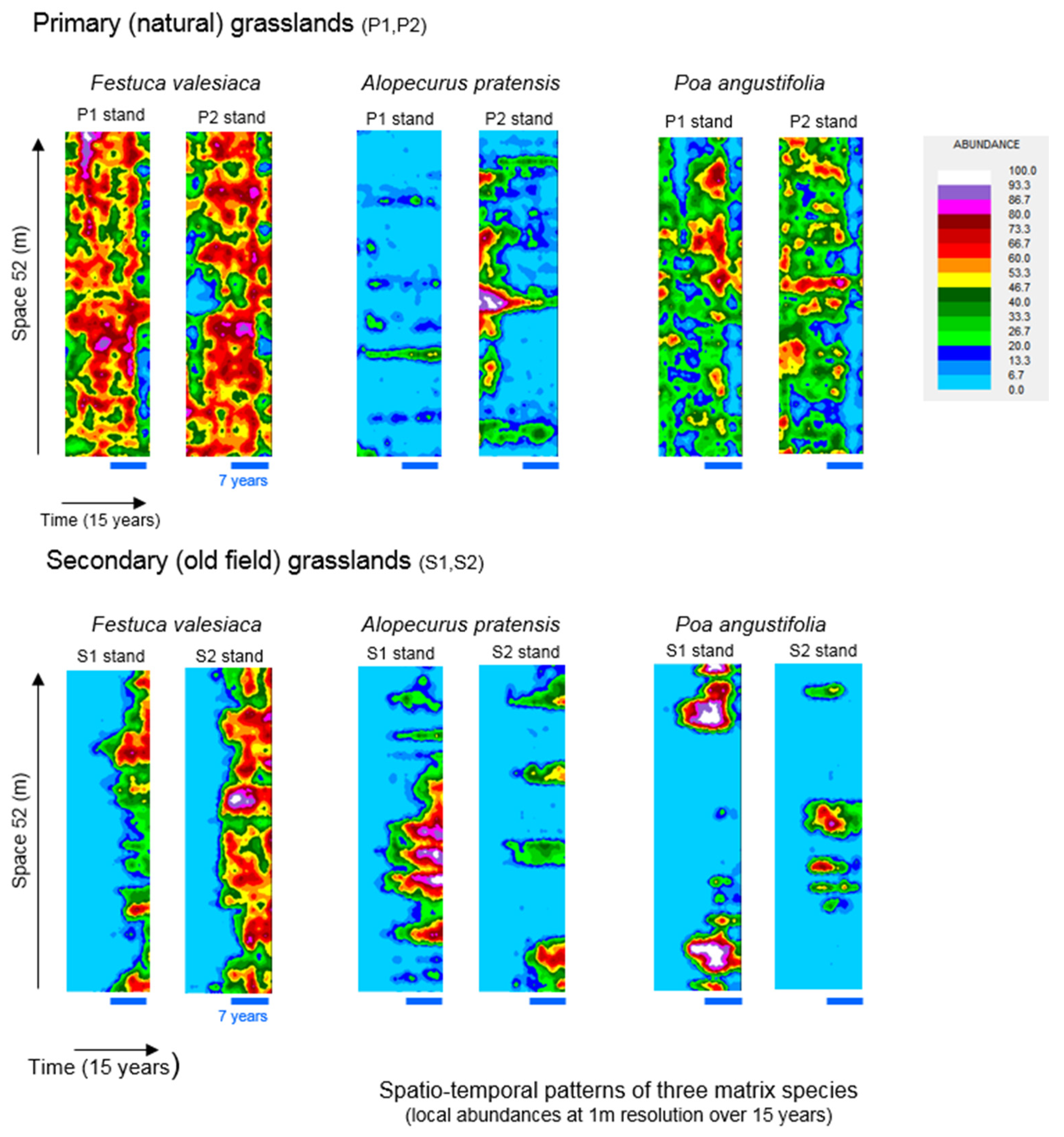
Figure 1. Fine-scale spatiotemporal patterns of the abundances of three matrix-forming grass species in primary and secondary grassland sites. The blue lines under the figures indicate the 7-year period (2019–2025) analyzed in this study.
Land 14 01736 g001
Figure 2. Spatial aggregation indices of the three matrix species over 7 years in primary (P1, P2) and secondary (S1, S2) grasslands.
Land 14 01736 g002
Figure 3. Overall (7-year) temporal associations of matrix species in primary (P1, P2) and secondary (S1, S2) grasslands. Note that analyses were performed at multiple spatial scales.
Land 14 01736 g003
Figure 4. Mean rates of change between years in the patterns of matrix species in primary (P1, P2) and secondary (S1, S2) grasslands, estimated (A) at a 10 cm resolution and (B) at a 20 cm resolution.
Land 14 01736 g004
Figure 5. Fine-scale distribution of local richness (A,C) and local combinations of matrix species (B,D) assessed at 10 cm (A,B) and 20 cm (C,D) resolutions. Matrix species combinations: ---, empty microsite; F--, only Festuca valesiaca is present; -A-, only Alopecurus pratensis is present; --P, only Poa angustifolia is present; FA-, Festuca valesiaca and Alopecurus pratensis are present; F-P, Festuca valesica and Poa angustifolia are present; -AP, Alopecurus pratensis and Poa angustifolia are present; FAP, all three species are present.
Land 14 01736 g005
Figure 6. Spatial variability in fine-scale subordinate species richness estimated at (A) 5 cm, (B) 10 cm and (C) 20 cm resolutions over the 7-year study period.
Land 14 01736 g006
Table 1. Characteristics of the matrix formed by the most abundant species in grasslands.
Primary GrasslandsSecondary Grasslands
spatial
dependence
nearly random patterns
or fine-scale patchiness
very strong aggregations
coarse scale patchiness
temporal
dependence
weak
appears at finer scales
strong
stronger at coarser scales
fine-scale
dynamics
(rate of changes)
high rate of exchanges
species specific rates
gain and loss rates balanced
high rate of exchanges
species specific rates
gain and loss rates imbalanced
spatial diversity
and co-occurrence
of matrix species
spatially variable patterns
of different 1-,2-,3-species
combinations
monodominant patches are typical
pattern of
subordinate
species richness
temporally stable
low spatial variability
temporally increasing
high spatial variability
potential mechanisms
effect of matrix
species on subordinates
weak pattern selection
homogeneous environment
spatially variable
temporally stable
strong pattern selection
heterogeneous environment
Disclaimer/Publisher’s Note: The statements, opinions and data contained in all publications are solely those of the individual author(s) and contributor(s) and not of MDPI and/or the editor(s). MDPI and/or the editor(s) disclaim responsibility for any injury to people or property resulting from any ideas, methods, instructions or products referred to in the content.