Article

Comparative Performance Analysis of Heterogeneous Ensemble Learning Models for Multi-Satellite Fusion GNSS-IR Soil Moisture Retrieval

1
Faculty of Geosciences and Engineering, Southwest Jiaotong University, Chengdu 611756, China
2
Cryosphere Research Station on the Qinghai-Tibet Plateau, State Key Laboratory of Cryospheric Science and Frozen Soil Engineering, Northwest Institute of Eco-Environment and Resources, Chinese Academy of Sciences, Lanzhou 730000, China
3
Institute of Plateau Meteorology, China Meteorological Administration, Chengdu 610072, China
*
Author to whom correspondence should be addressed.
Land 2025, 14(9), 1716; https://doi.org/10.3390/land14091716 (registering DOI)
Submission received: 9 June 2025 / Revised: 1 August 2025 / Accepted: 21 August 2025 / Published: 25 August 2025

Abstract

Given the complexity of near-surface soil moisture retrieval, a single machine learning algorithm often struggles to capture the intricate relationships among multiple features, resulting in limited generalization and robustness. To address this issue, this study proposes a multi-satellite fusion GNSS-IR soil moisture retrieval method based on heterogeneous ensemble machine learning models. Specifically, two heterogeneous ensemble learning strategies (Bagging and Stacking) are combined with three base learners, Back Propagation Neural Network (BPNN), Random Forest (RF), and Support Vector Machine (SVM), to construct eight ensemble GNSS-IR soil moisture retrieval models. The models are validated using data from GNSS stations P039, P041, and P043 within the Plate Boundary Observatory (PBO) network. Their retrieval performance is compared against that of individual machine learning models and a deep learning model (Multilayer Perceptron, MLP), enabling an optimized selection of algorithms and model architectures. Results show that the Stacking-based models significantly outperform those based on Bagging in terms of retrieval accuracy. Among them, the Stacking (BPNN-RF-SVM) model achieves the highest performance across all three stations, with R of 0.903, 0.904, and 0.917, respectively. These represent improvements of at least 2.2%, 2.8%, and 2.1% over the best-performing base models. Therefore, the Stacking (BPNN-RF-SVM) model is identified as the optimal retrieval model. This work aims to contribute to the development of high-accuracy, real-time monitoring methods for near-surface soil moisture.

1. Introduction

Near-surface soil moisture (SMC) has long been a focal point in climate and land-atmosphere interaction studies due to its critical role in agricultural management, water resource allocation, climate prediction, and disaster early warning [1,2]. It also forms a fundamental basis for ecological sustainability and environmental monitoring. Therefore, developing efficient and reliable methods for retrieving soil moisture is of great significance. Traditional soil moisture measurement approaches typically involve in situ operations, which are labor-intensive, costly, and constrained by limited spatial and temporal resolution, making them unsuitable for large-scale applications. In recent years, Global Navigation Satellite System (GNSS) remote sensing technology has developed rapidly. Among its derivatives, GNSS Reflectometry (GNSS-R) has emerged as a novel approach for retrieving soil moisture [3]. Ground-based GNSS-R systems utilize dedicated receivers to capture GNSS signals reflected from the Earth’s surface and directly analyze signal characteristics such as intensity, delay, and polarization to retrieve surface parameters.
Kavak et al. [4] were among the first to investigate the sensitivity of GNSS-reflected signals to soil moisture content. Zavorotny et al. [5,6] further demonstrated the potential of GNSS-R for soil moisture retrieval through simulation experiments, which were later validated using both ground-based and airborne GNSS-R campaigns. The National Aeronautics and Space Administration (NASA) carried out an airborne GPS-R experiment called SMEX02 to evaluate the potential of using GPS-R signals for soil moisture estimation. The data obtained from this campaign were successfully used for soil moisture estimation [7,8,9]. Additionally, the impact of antenna polarization on GNSS-R soil moisture retrieval was tested [10]. The European Space Agency (ESA) and Starlab carried out the LEiMON (Land Monitoring Using Navigation Signals) and GRASS (GNSS Reflectometry for Biomass Analysis) experiments in 2009 and 2011, respectively. These ground-based and airborne GNSS-R experiments explored the effects of soil moisture, surface roughness, and vegetation parameters on GPS-reflected signals [11]. Egido et al. conducted low-altitude airborne tests, revealing that the polarized reflectivity ratio served as the most reliable soil moisture indicator under moderate surface roughness, achieving a correlation coefficient of 0.93 [12]. After the successful deployment of NASA’s CYGNSS mission, multiple data processing techniques have been utilized on its observations [13,14,15], facilitating global soil moisture estimation at a spatial resolution of 36 × 36 km2 with a root mean square error of 0.07 cm3/cm3 [16].
However, dedicated receivers for GNSS-R are often costly and require complex maintenance, limiting their large-scale application. To address this, Larson et al. were the first to propose the GNSS Interferometric Reflectometry (GNSS-IR) technique. This method does not require specialized equipment; instead, it uses standard geodetic GNSS receivers to simultaneously capture both direct and reflected signals. By analyzing the signal-to-noise ratio (SNR) fluctuations caused by the interference between the two signals, surface parameters can be retrieved [17,18,19]. Larson was the first to show that soil moisture has a strong influence on the amplitude and phase behavior of SNR oscillations observed in GPS reflected signals [18]. Since then, an increasing number of researchers have explored the use of GNSS-IR for soil moisture retrieval. Zavorotny et al. utilized delayed phase signals for soil moisture estimation and found this approach to be more stable than amplitude-based methods [20]. Chew et al. later verified a distinct linear relationship between the initial phase of reflected GPS signals and surface soil moisture through experiments on bare soil [21]. In recent years, machine learning techniques have been increasingly employed for soil moisture monitoring, leading to the development of various algorithms aimed at improving retrieval precision. Li et al. proposed a Helmert variance component estimation (HVCE) method to weight and combine dual-frequency carrier phase data, effectively accounting for the differences and complementarity between satellite signal frequencies [22]. They developed both linear and machine learning-based retrieval models, and the results showed that HVCE-fused dual-frequency data significantly enhanced the retrieval accuracy, with machine learning models outperforming traditional linear models. To mitigate the influence of environmental noise, Liang et al. proposed a phase correction model combined with a BP neural network to further improve single-satellite accuracy [23]. Subsequently, Sun et al. developed an SVM model optimized through a genetic algorithm, leading to further improvements in retrieval accuracy [24]. However, due to the temporal and spatial differences among satellites, single-satellite retrieval methods often suffer from low stability. To overcome this issue, Ren et al. constructed a retrieval model using least squares support vector machines combined with multi-satellite data fusion, showing that this approach achieved higher accuracy than models relying on single-satellite observations [25]. To further reduce the impact of environmental noise on bare-soil retrieval accuracy, Xian et al. designed a multi-layer perceptron (MLP)-based model that incorporates diverse features, filters out abnormal satellite data using a threshold-based strategy, and builds a retrieval framework through multi-satellite fusion [26]. Experimental findings indicated that the model achieved markedly better performance compared to traditional linear approaches. Nevertheless, due to the complexity of soil moisture prediction, individual machine learning models still suffer from inherent uncertainty, such as sensitivity to parameter settings and limited generalization capability. A single algorithm may struggle to capture the complex relationships and differences across diverse datasets, thereby limiting prediction accuracy.
Ensemble learning is a powerful technique that enhances the accuracy of individual learners while minimizing modeling uncertainties. This approach has been utilized in areas like landslide detection, medical image analysis, and land cover classification, with research indicating that ensemble models often deliver more precise predictions compared to individual learners. Ensemble learning is generally categorized into homogeneous and heterogeneous approaches. For example, Youssef et al. developed a homogeneous ensemble using decision trees to create a landslide susceptibility map for the Wadi Tayyah basin [27], while Li et al. implemented a stacked heterogeneous ensemble combining CNN and RNN to map landslide susceptibility in China’s Three Gorges region [28]. Despite its demonstrated versatility across multiple domains, the potential of ensemble learning for soil moisture retrieval remains insufficiently investigated.
To address the aforementioned challenges, this study proposes a novel multi-satellite fusion GNSS-IR soil moisture retrieval method based on heterogeneous ensemble machine learning models. Building upon conventional GNSS-IR retrieval algorithms, the proposed approach utilizes phase features derived from multiple satellites and multiple arcs as input data. Three classical base learners (RF, BPNN, and SVM) are first employed to construct individual soil moisture retrieval models. These models are then integrated using two ensemble learning strategies, Bagging and Stacking, resulting in a series of ensemble-based retrieval models. The proposed models were evaluated using GNSS observations obtained from the Plate Boundary Observatory (PBO) network, focusing on data collected at stations P041 (2012), P039 (2017), and P043 (2015). To further evaluate performance, a Multilayer Perceptron (MLP) deep learning model is introduced for comparison. A systematic analysis is conducted to compare the prediction accuracy and generalization capabilities of individual machine learning models, deep learning models, and ensemble learning models.

2. Methodology

2.1. Technical Processes

In this research, GNSS observation and navigation data are analyzed to extract parameters such as signal-to-noise ratio (SNR), elevation angle, and azimuth. For each satellite, the daily SNR measurements are segmented into individual ascending or descending arcs according to variations in the elevation angle. Phase-related feature parameters are then derived from each arc for subsequent analysis. Then, Bagging and Stacking heterogeneous ensemble learning algorithms are used to combine RF, BPNN, and SVM models to build prediction models with stronger generalization and better robustness. The advantages of different ensemble strategies and methods are analyzed to identify the optimal prediction model. The specific experimental procedure is shown in Figure 1.

2.2. GNSS-IR Soil Moisture Retrieval Principle

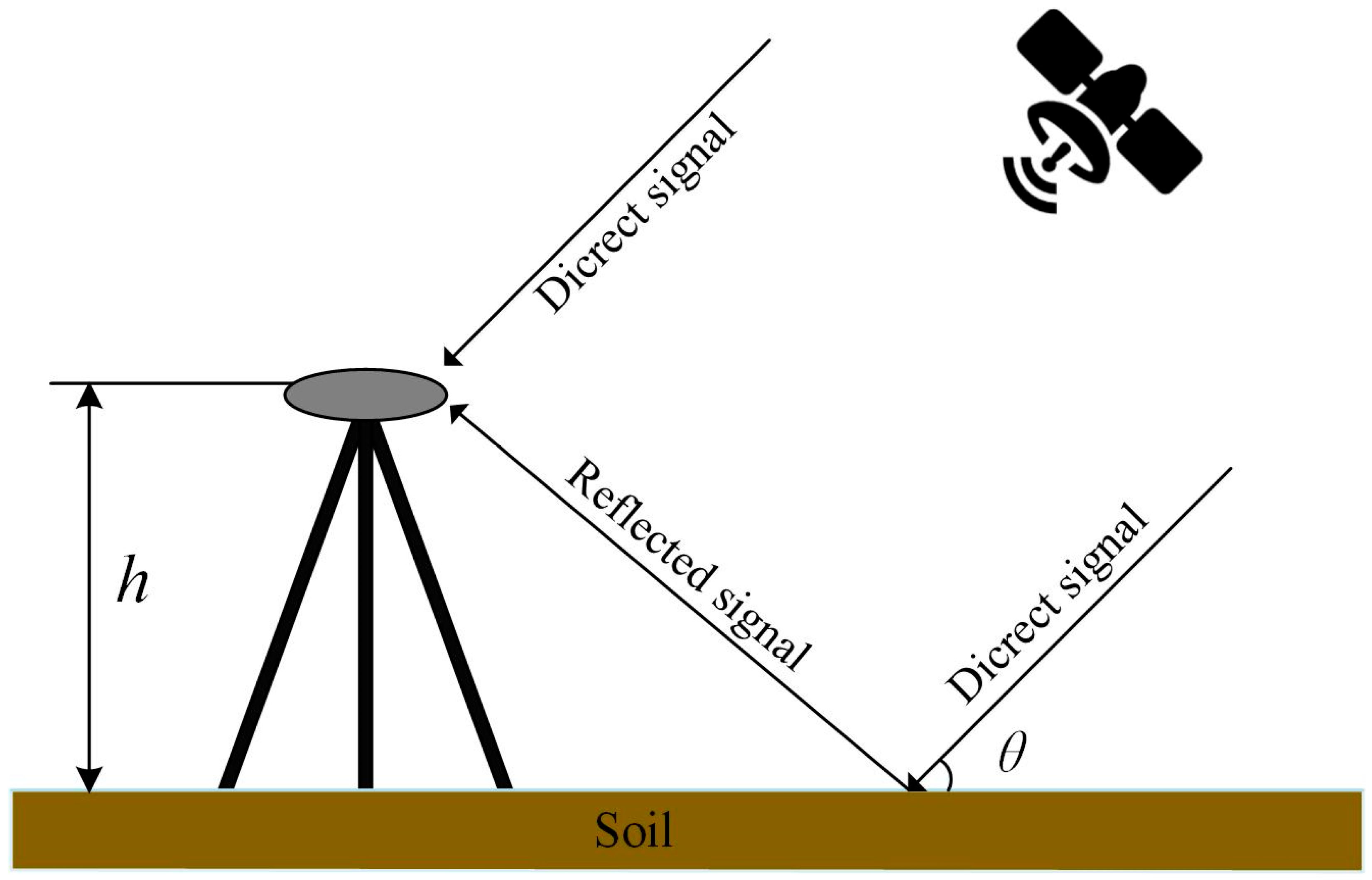
Multipath effects cause the receiver antenna to capture both direct and reflected signals at the same time, leading to a phase difference between these signals. Figure 2 depicts the geometric configuration, where h indicates the vertical distance from the antenna phase center to the reflective surface, and θ represents the satellite’s elevation angle.
The superposition of the direct and reflected signals results in interference, forming a composite signal. Under a simplified model, the Signal-to-Noise Ratio (SNR) of this composite signal can be expressed as [18,29],
SNR 2 = A m 2 + A d 2 + 2 A d A m cos φ
In this context, Ad and Am denote the amplitudes of the direct and reflected signals, respectively, while φ indicates the phase offset between the two. Prior to feature extraction, a low-order polynomial is used to fit and eliminate the direct signal portion from the original SNR data, resulting in a residual dSNR signal that primarily captures the multipath-induced reflections [30].
d S N R = A m cos 4 π h λ sin θ + φ m
In this context, h refers to the vertical distance from the GNSS antenna’s phase center to the reflecting surface, θ represents the satellite’s elevation angle, and λ denotes the GNSS signal’s wavelength. Am and φm correspond to the amplitude and phase feature parameters, respectively. By defining t = sinθ and f = 2h/λ, Equation (2) can be further reduced and simplified accordingly,
d S N R = A m cos 2 π f t + φ m
Subsequently, the Lomb-Scargle periodogram (LSP) is applied to each SNR arc to extract the dominant frequency component, denoted as f. The resulting dSNR sequences are then modeled using a cosine function, and nonlinear least squares fitting is employed to estimate key parameters, including frequency, amplitude, and phase [31]. Previous studies have shown that the phase parameter is closely linked to soil moisture levels. Therefore, this research emphasizes the phase feature as the principal variable for retrieving soil moisture [21].

2.3. Heterogeneous Integrated Learning Model Foundation Learner

2.3.1. Back Propagation Neural Network

The Back Propagation Neural Network (BPNN), a typical feedforward multilayer neural network, possesses strong nonlinear modeling and adaptive learning capabilities. It primarily learns the nonlinear mapping between input features and observed values by training on various feature parameters. Compared with traditional linear models, BPNN introduces nonlinear activation functions (such as Sigmoid or ReLU) in the hidden layers to perform nonlinear transformations on the input signals. By stacking these nonlinear mappings through a multilayer network structure and optimizing the weights and biases of each layer via the backpropagation algorithm, the network is capable of capturing complex nonlinear relationships between inputs and outputs. This enables BPNN to effectively model nonlinear patterns in data, with strong generalization ability and a built-in mechanism for error correction through backpropagation [32].

2.3.2. Random Forest

Random Forest (RF) makes predictions by aggregating the votes or average results of multiple decision trees. It has strong nonlinear modeling capability and resistance to overfitting. RF fully utilizes multidimensional features by building many decision tree models to explore complex relationships among features, thereby improving retrieval accuracy. At the same time, RF shows strong robustness in handling high-dimensional data and small sample sizes. It can automatically evaluate the importance of each input feature, optimizing feature selection and enhancing the model’s generalization ability [33,34].

2.3.3. Support Vector Machine

Support Vector Machine (SVM) is a supervised learning method based on statistical learning theory, known for its strong generalization ability and capacity to handle high-dimensional data. By using kernel functions, SVM can effectively capture nonlinear relationships between features and build robust retrieval models. Compared to traditional regression methods, SVM maintains high prediction accuracy even with limited samples or noisy data, and it is less sensitive to outliers. The robustness and stability of the retrieval model can be further improved by selecting appropriate kernel functions and optimizing parameters [35].

2.3.4. Multilayer Perceptron

The Multilayer Perceptron (MLP) is a fundamental feedforward neural network model composed of an input layer, one or more hidden layers, and an output layer. Each layer consists of multiple neurons, and the layers are hierarchically connected through weighted links. MLP processes data through forward propagation: the input layer receives raw data, and each neuron in the hidden layer computes a weighted sum of the previous layer’s outputs, followed by a nonlinear activation function (e.g., ReLU or Sigmoid) to perform feature abstraction and transformation. The output layer then produces the final result. During training, the model employs the backpropagation algorithm to compute gradients based on a loss function (such as mean squared error or cross-entropy) and uses gradient descent to iteratively optimize the weights and biases of each layer, enabling the model to gradually approximate the underlying data patterns. MLP has strong nonlinear fitting capabilities and can learn complex mappings within the data. Its multilayer structure facilitates hierarchical feature learning, progressively extracting high-level abstract features from low-level ones. This makes it well-suited for a wide range of tasks, including classification and regression [36].

2.4. Heterogeneous Integrated Learning Algorithms

2.4.1. Bagging Integrated Learning Algorithm

Bagging (Bootstrap Aggregating) is an ensemble learning algorithm that builds more robust classifiers by combining multiple base models [37]. The core idea of this algorithm is to introduce randomness during the construction of the ensemble model, which reduces the variance of the base models and improves model stability and prediction accuracy [33,38]. One advantage of Bagging is that it can effectively improve the weaknesses of base models without changing their mathematical structure when addressing a single problem. Bagging can be divided into homogeneous and heterogeneous types [39]. In homogeneous Bagging, the base learners are of the same model type, such as decision trees or neural networks. In contrast, heterogeneous Bagging includes more diverse base learners, which can be different models like SVM [35], RF [33], and BPNN. Heterogeneous Bagging can enhance generalization ability and prediction performance by increasing model diversity and robustness [37]. In this study, we chose the heterogeneous Bagging ensemble algorithm to integrate the three base learners described in Section 2.3. Its working mechanism involves training each base learner independently on the original training dataset to form separate base models. These trained base learners then predict all grid units. Finally, the predictions from all base learners are combined by averaging or voting to obtain the final prediction. The framework of the Bagging algorithm is shown in Figure 3.

2.4.2. Stacking Integrated Learning Algorithm

Stacking, as an advanced ensemble learning framework [40], effectively combines the strengths of multiple models to build a superior, higher-accuracy, and more robust generalized model [41]. The Stacking algorithm, proposed by Smyth and Wolpert [42], uses a multi-layer structure, typically two layers. In this study, a two-layer structure is adopted. In the first layer, predictions from n different base models are aggregated into new features, which serve as input data for the second-layer meta-model. Subsequently, the second-layer meta-model is trained using this newly generated feature dataset to yield the final output. Initially, the entire sample dataset is divided into five smaller subsets. Each subset is sequentially designated as the validation set, while the remaining four subsets are used to train the n base models. This five-fold cross-validation procedure is conducted to construct the secondary training dataset. The objective of this approach is to prevent directly utilizing the base model outputs as inputs for the meta-model, thereby mitigating the potential for overfitting. Next, the outputs from the five-fold cross-validation of the first-layer base models are combined to create a new feature dataset. This dataset serves as the input for training the second-layer meta-model (LR model) [43]. After training, the entire set of grid cell data is passed through the base models to generate predictions, which are then provided to the trained meta-models. The average of these five-fold cross-validation results is used to produce enhanced grid features, resulting in an updated grid dataset. This refined dataset is then input into the second-layer meta-model to derive the final prediction outcomes. The overall structure of the Stacking algorithm is depicted in Figure 4.

3. Study Area and Data

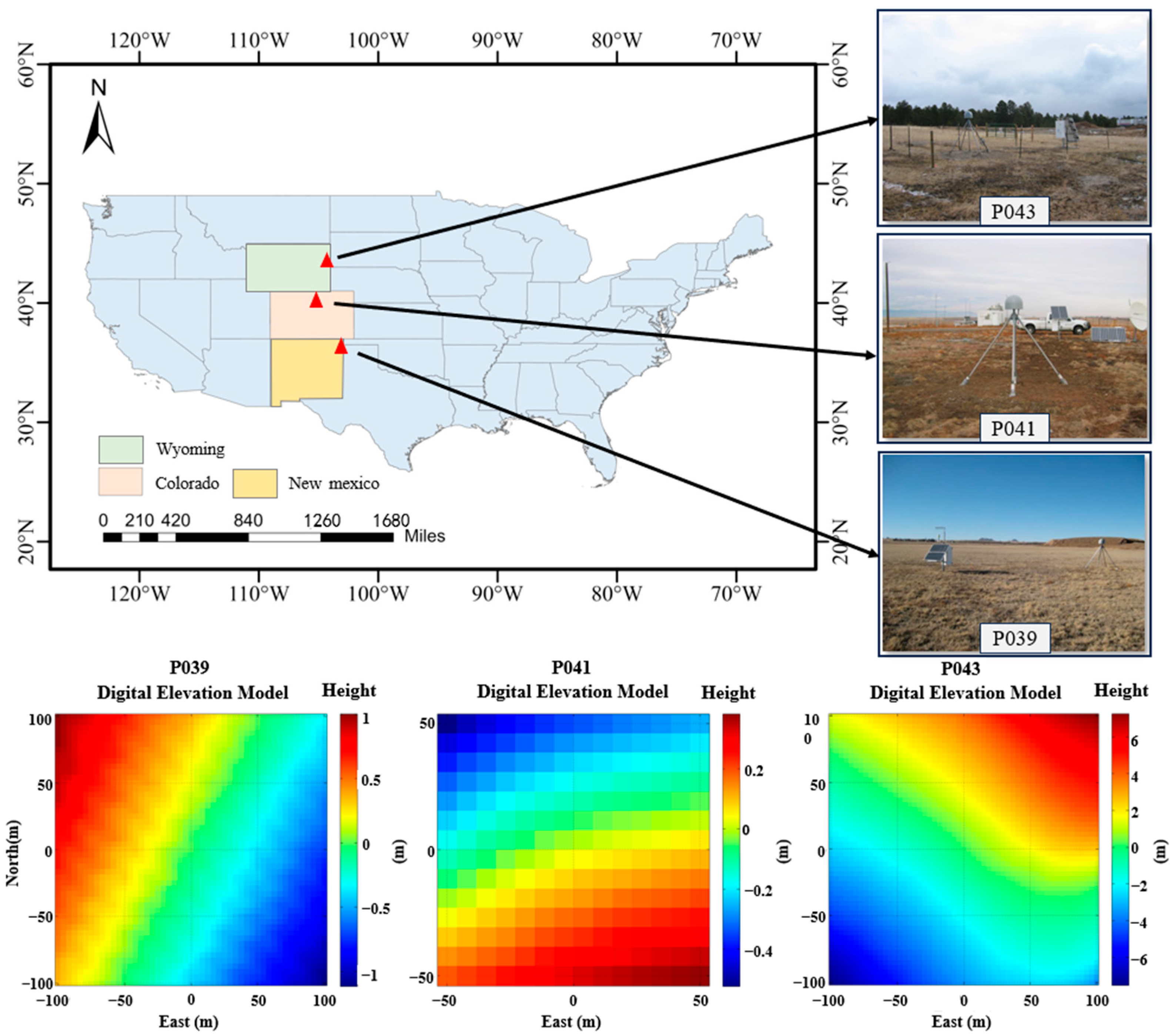
This research carries out experimental analysis based on GNSS station data and corresponding soil moisture reference measurements obtained from the Plate Boundary Observatory (PBO). To ensure the availability of continuous soil moisture reference data for validation, we selected data from station P041 (105.1943° W, 39.9495° N) for the year 2012, spanning day of year (DOY) 98–265, and from station P043 (104.1857° W, 43.8811° N) for the year 2015, covering DOY 142–314. Additionally, to evaluate the generalization performance of the models, data from station P039 (103.154° W, 36.4481° N), located in a nearby region with dense vegetation, were used for the year 2017, covering DOY 20–302. The areas surrounding all three experimental sites are flat and open, with no major obstructions, making them suitable for soil moisture retrieval studies. Figure 5 presents schematic views of the surrounding environments and the digital elevation model (DEM) for stations P039, P041, and P043.
In this study, SNR observations were recorded at 15 s intervals. Since lower satellite elevation angles tend to intensify multipath interference and cause greater signal distortion at the receiver antenna [44,45], this study utilizes the first Fresnel zone (FFZ) to define the effective reflecting surface at each observation station [18]. Accordingly, L2 band SNR data corresponding to elevation angles between 5° and 25° were selected for analysis.
Figure 6 presents the time series of observed SMC and precipitation for station P039 (2017), station P041 (2012), and station P043 (2015), displayed using line graphs for SMC and bar charts for precipitation. As depicted in Figure 6, around 10 notable rainfall events were observed at station P041, whereas stations P043 and P039 encountered more frequent and intense precipitation, which led to relatively higher overall soil moisture content levels. During precipitation events, SMC increased notably. Sustained rainfall led to a pronounced nonlinear rise in SMC, whereas a decline or cessation of precipitation was followed by a decreasing trend in SMC. These trends suggest that rainfall is the main factor causing sudden variations in soil moisture. The selected time periods for all three stations encompass substantial variations in both precipitation and soil moisture, making the datasets well-suited for soil moisture analysis.

4. Results

4.1. Soil Moisture Retrieval Results of Baseline Machine Learning and Deep Learning Models

This study developed soil moisture retrieval models utilizing BPNN, RF, SVM, and MLP algorithms, based on phase data extracted from all accessible satellite arcs at stations P039, P041, and P043. To construct robust and stable baseline models, a grid search approach was employed to optimize the hyperparameter spaces of the four models. Compared to manual tuning, this method improves both optimization efficiency and accuracy while reducing model uncertainty. The final optimized parameter settings for each base model are summarized in Table 1.
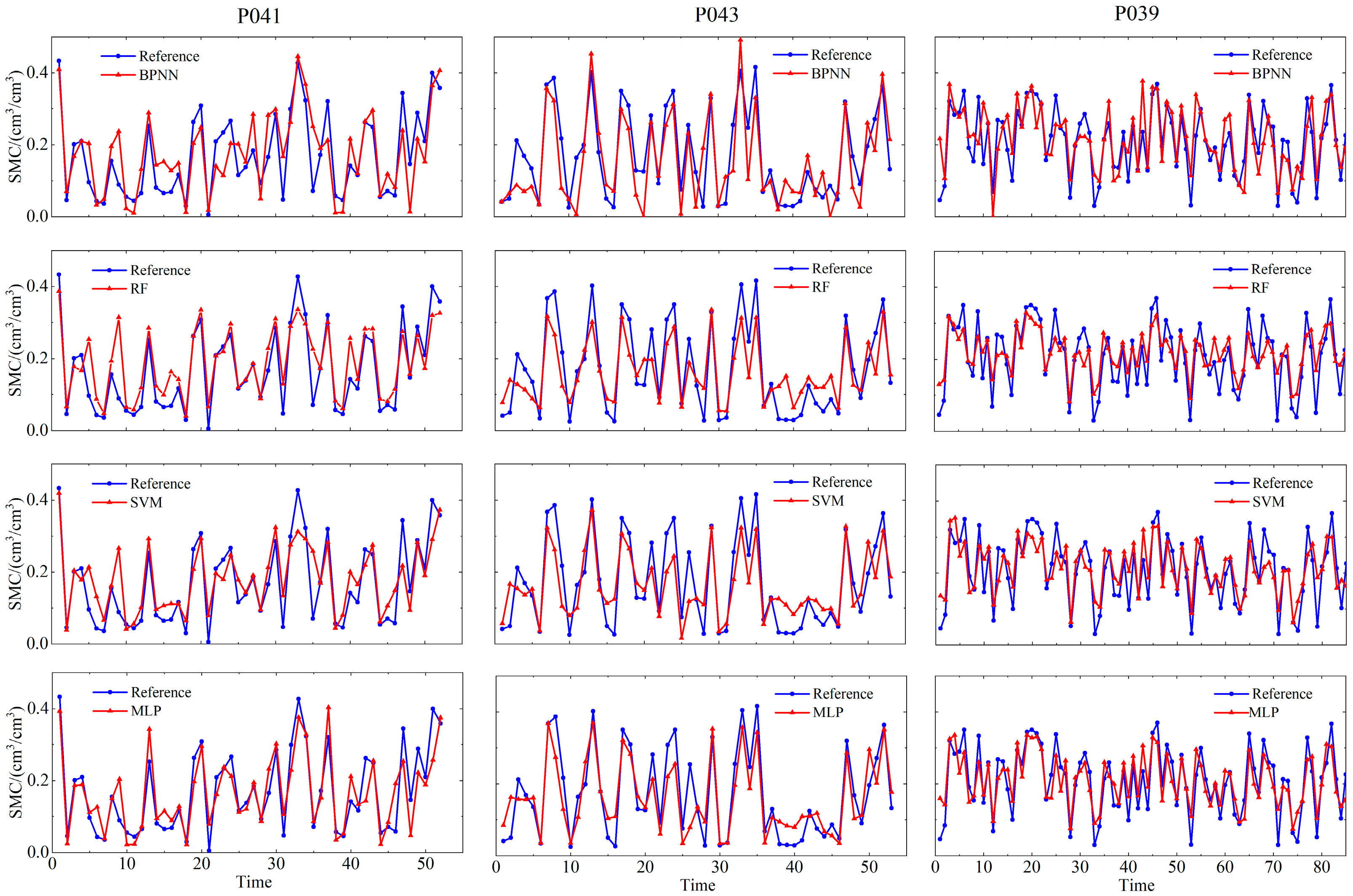
Figure 7 displays the soil moisture retrieval outcomes at stations P039, P041, and P043 obtained from models built using BPNN, RF, SVM, and MLP. As shown in the figure, all four models effectively capture the general variation trends of the reference soil moisture values. However, among them, the BPNN model exhibits more aggressive behavior, with larger deviations observed at certain time points. The RF and SVM models accurately reflect the overall soil moisture trends, but their retrievals tend to be conservative. In particular, both models struggle to capture peak values during periods of rapid soil moisture change. The MLP model, as a deep learning architecture with two hidden layers, performs weighted summations on the outputs of the preceding layer and applies nonlinear activation functions (e.g., ReLU or Sigmoid) to abstract and transform features. Owing to its stronger nonlinear fitting capability, MLP provides more stable retrievals across the three stations and demonstrates superior accuracy in predicting soil moisture peaks compared to traditional machine learning models.

4.2. Integrated Machine Learning Model Soil Moisture Retrieval Results

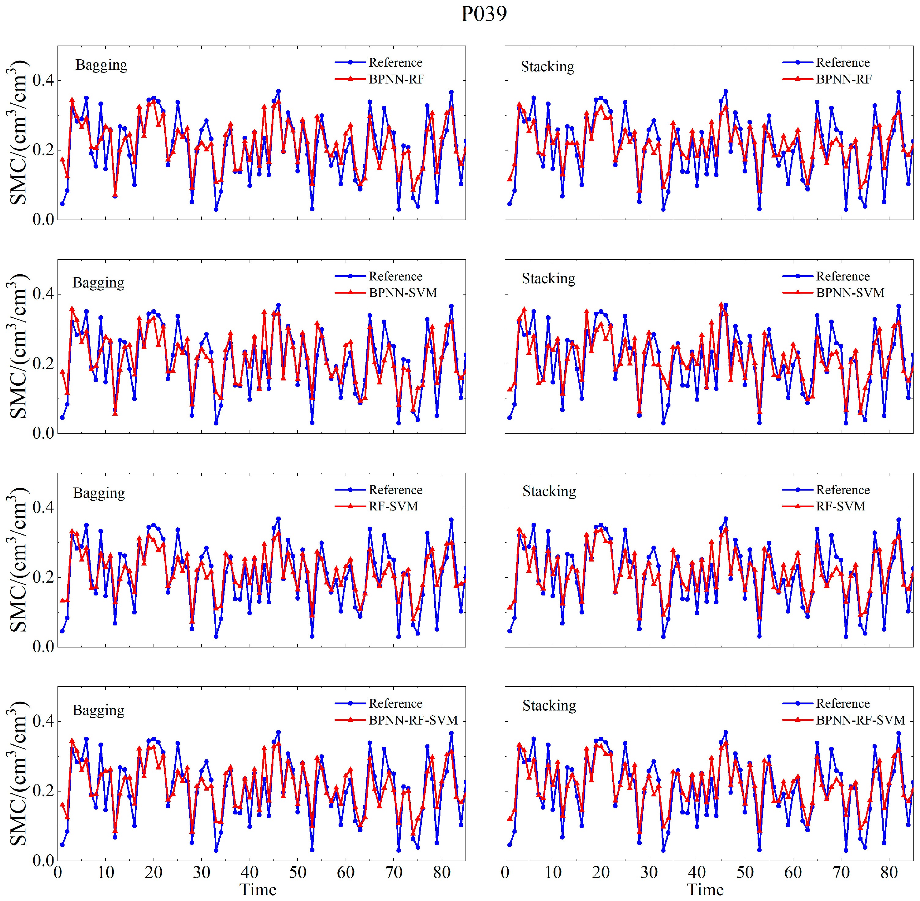
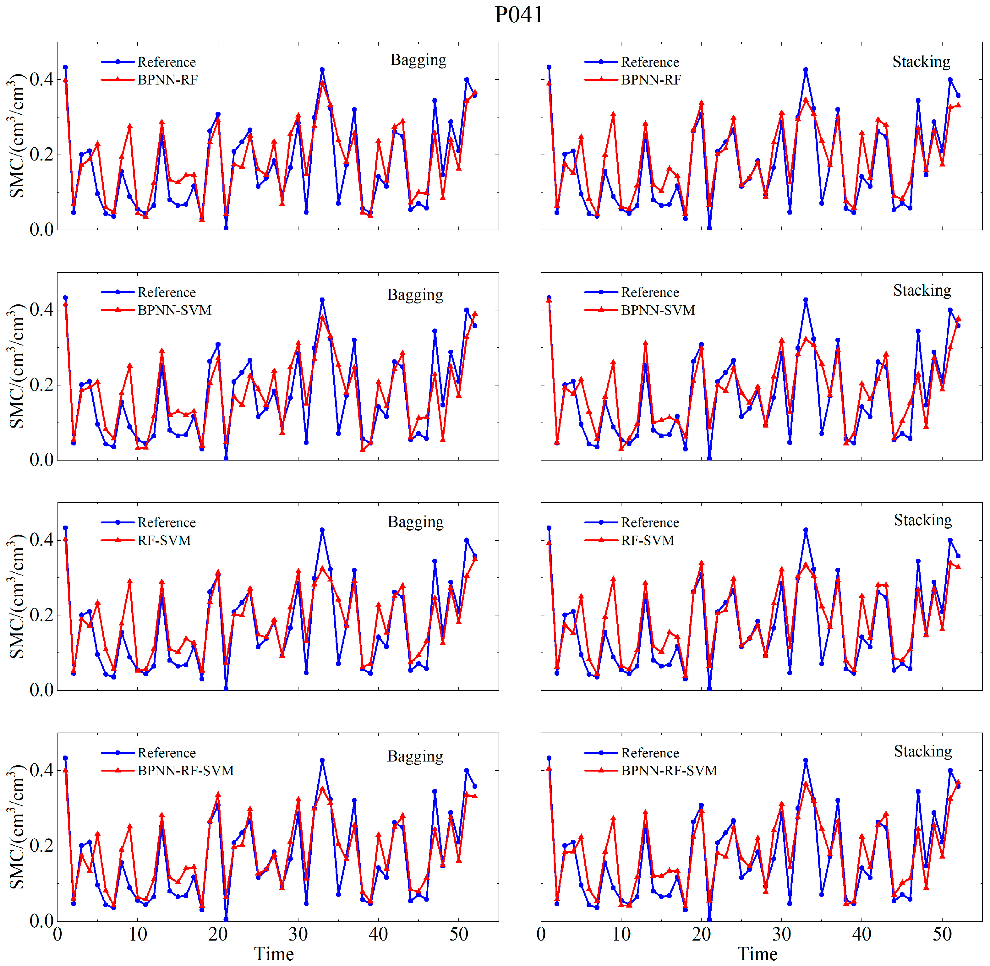
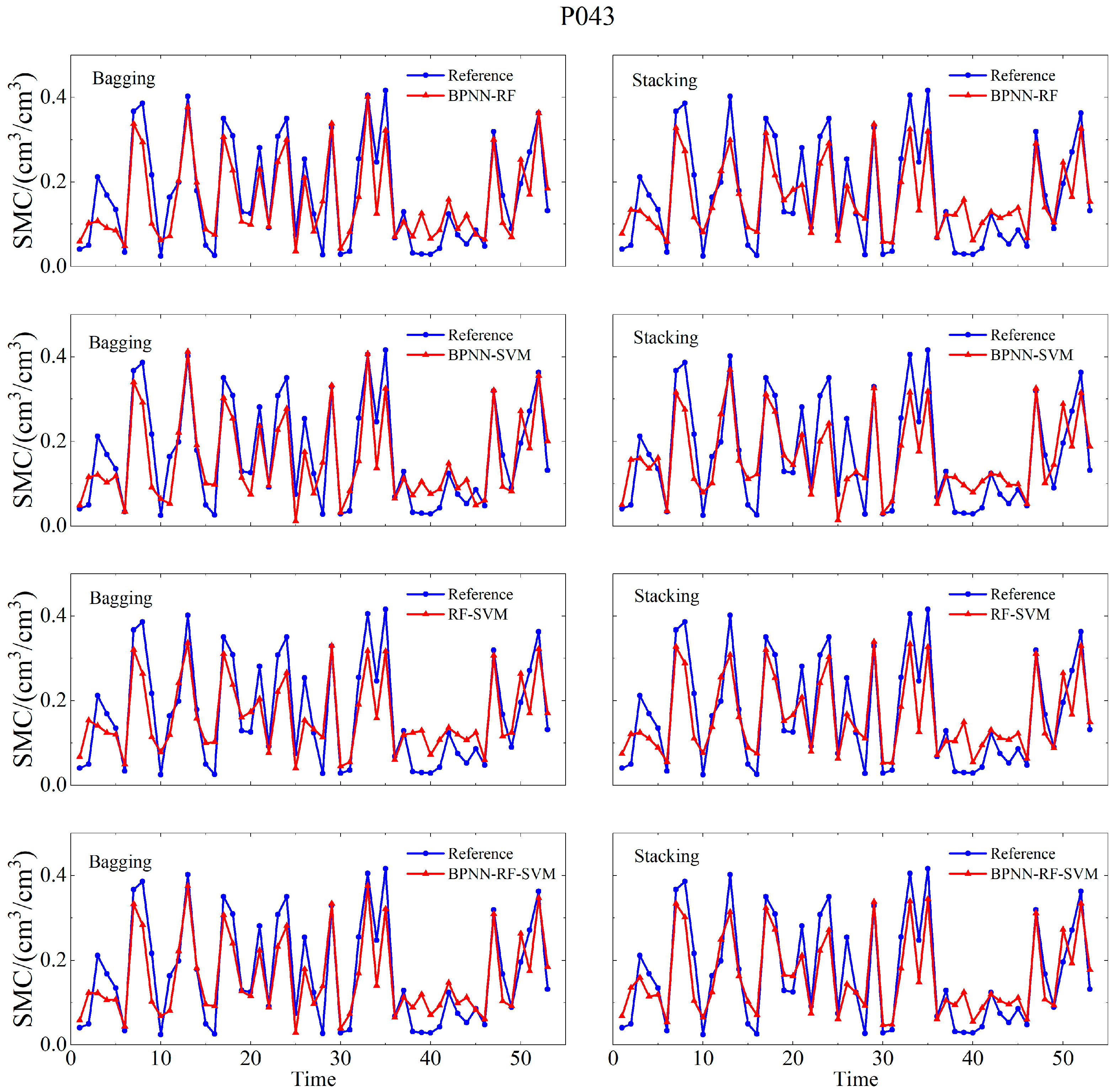
Figure 8, Figure 9 and Figure 10 display the soil moisture retrieval outcomes of ensemble models based on Bagging and Stacking algorithms at stations P039, P041, and P043, respectively. As shown in the figures, both ensemble approaches significantly outperform the individual models, yielding more stable retrievals with better overall fit. The Bagging algorithm improves model accuracy and robustness by reducing the bias and variance of individual models while preserving their respective strengths. In contrast, the Stacking algorithm employs a meta-learner to further learn and optimize the outputs of base models, effectively leveraging the complementary advantages among them. This results in enhanced retrieval accuracy and improved generalization performance of the overall model.

5. Discussion

5.1. Evaluation of Retrieval Accuracy for Soil Moisture Results Across Different Models

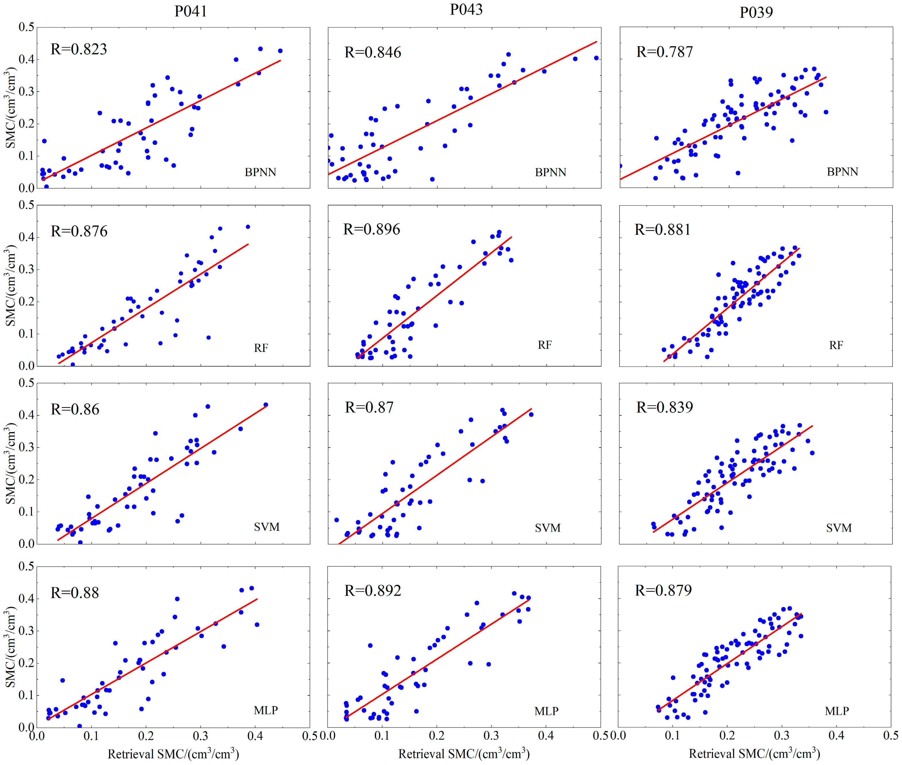
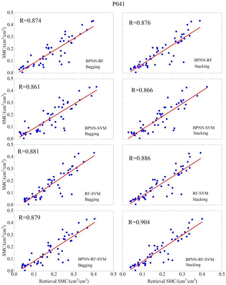
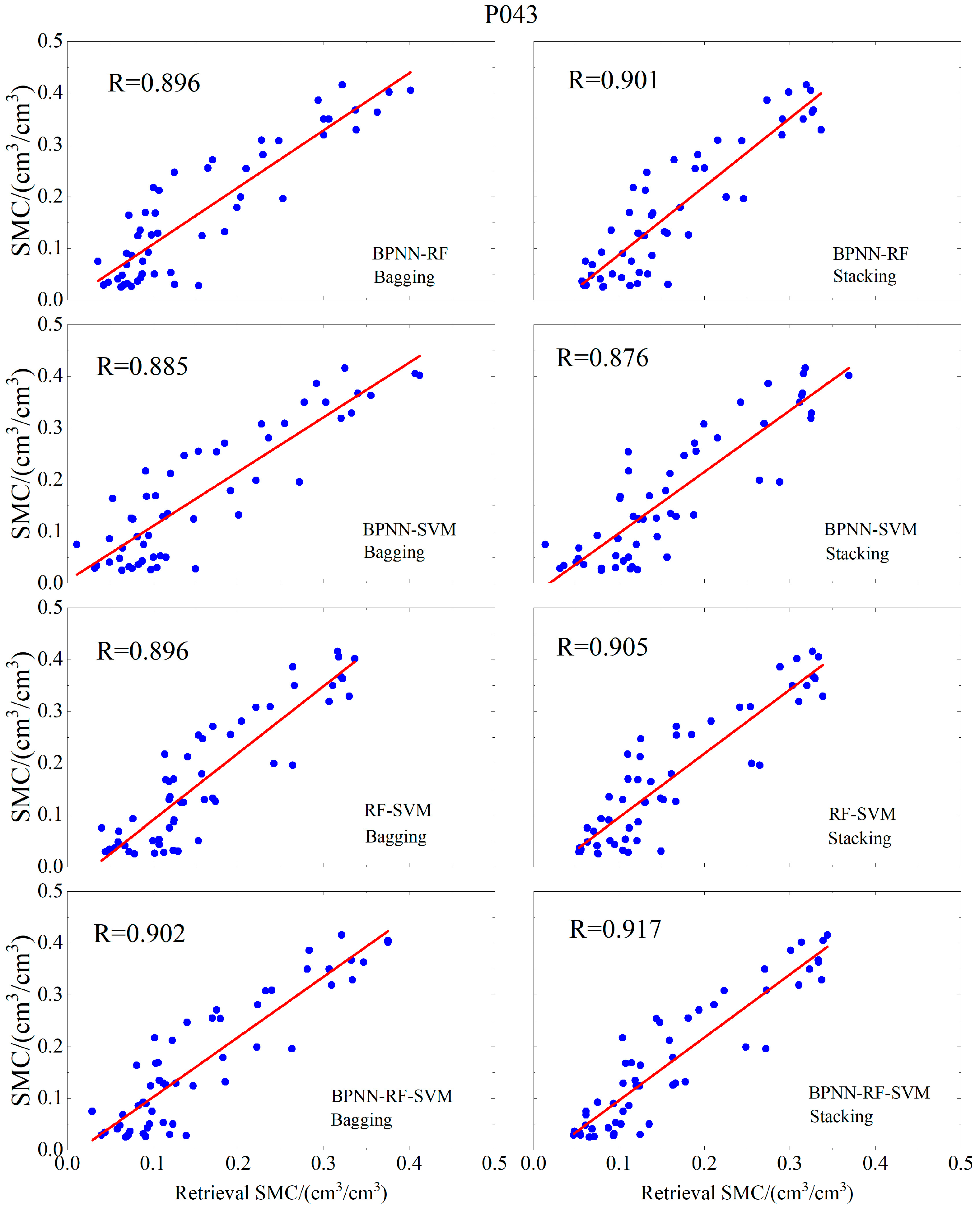
To further assess the effectiveness of various models in multi-satellite fusion soil moisture retrieval, this study employs three evaluation metrics: R, root mean square error (RMSE), and mean absolute error (MAE) to analyze and compare the retrieval outcomes. As shown in Figure 11, Figure 12, Figure 13 and Figure 14, all individual learning models and ensemble models, except BPNN, achieved R greater than 0.8, indicating strong retrieval performance. For station P039, the R values of the optimized machine learning models (BPNN, RF, and SVM) were 0.787, 0.881, and 0.839, the RMSE values were 0.0588, 0.0501, and 0.051, and the MAE values were 0.0449, 0.0421, and 0.0421, respectively. At station P041, the R values were 0.823, 0.876, and 0.860, RMSE values were 0.0683, 0.0598, and 0.061, and MAE values were 0.0547, 0.0409, and 0.0441, respectively. For station P043, the R values were 0.846, 0.896, and 0.870, RMSE values were 0.0717, 0.0621, and 0.0643, and MAE values were 0.0577, 0.0529, and 0.0534, respectively. Among the three machine learning models, RF achieved the highest retrieval accuracy across all stations. In contrast, BPNN exhibited considerable variation in retrieval performance across the three sites, with the poorest results observed at station P039, which is characterized by dense vegetation. This suggests that the generalization capability of the BPNN model is relatively limited. The MLP model demonstrated more stable performance across all stations. For station P039, its R, RMSE, and MAE were 0.879, 0.045, and 0.0384, respectively. For station P041, the values were 0.880, 0.055, and 0.041. And for station P043, they were 0.892, 0.0576, and 0.0462. MLP outperformed both BPNN and SVM and achieved comparable accuracy to RF, indicating strong generalization ability.
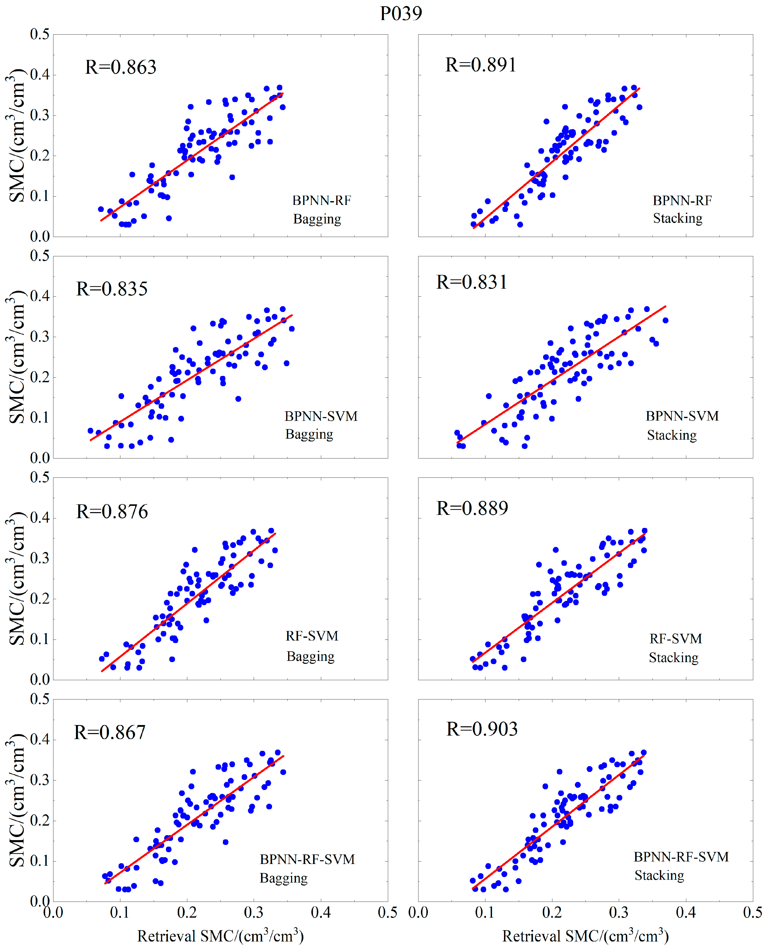
For the Bagging ensemble models (BPNN-RF, BPNN-SVM, RF-SVM, and BPNN-RF-SVM), the R values at station P039 were 0.863, 0.835, 0.876, and 0.867, the RMSE values were 0.0484, 0.051, 0.0486, and 0.0479, and the MAE values were 0.0383, 0.0397, 0.0408, and 0.0386, respectively. At station P041, the R values were 0.874, 0.861, 0.881, and 0.879, RMSE values were 0.058, 0.0599, 0.0582, and 0.0572, and MAE values were 0.0435, 0.0465, 0.0402, and 0.0424. For station P043, the R values were 0.896, 0.885, 0.896, and 0.902, RMSE values were 0.0577, 0.0596, 0.0613, and 0.0572, and MAE values were 0.0469, 0.0481, 0.0526, and 0.0467. At station P039, the ensemble models exhibited retrieval accuracies slightly lower than the RF model but showed significant improvement compared to BPNN and SVM models. At station P041, the R of the RF-SVM and BPNN-RF-SVM ensembles increased by at least 0.5% and 0.3%, respectively, compared to the individual machine learning models. At station P043, the BPNN-RF-SVM ensemble improved the R by at least 0.6% over the single models. It is noteworthy that the BPNN-RF and BPNN-SVM ensembles at stations P041 and P043 showed R slightly below that of RF alone, yet still outperformed the BPNN and SVM models, likely due to the relatively poor retrieval performance of the BPNN base model. Compared to the MLP model, the Bagging ensembles did not demonstrate significant improvement in retrieval accuracy across all three stations. Overall, the Bagging ensemble algorithm can enhance the retrieval accuracy of single machine learning models when appropriate base models are selected; however, it does not provide a marked advantage over deep learning models.
For the Stacking ensemble models (BPNN-RF, BPNN-SVM, RF-SVM, and BPNN-RF-SVM), the R values at station P039 were 0.891, 0.831, 0.889, and 0.903, RMSE values were 0.0484, 0.0518, 0.0452, and 0.0446, and MAE values were 0.0417, 0.0439, 0.0378, and 0.0371, respectively. At station P041, the R values were 0.877, 0.866, 0.886, and 0.904, RMSE values were 0.0598, 0.0598, 0.0572, and 0.0522, and MAE values were 0.0411, 0.0436, 0.0395, and 0.0379. For station P043, the R values were 0.901, 0.876, 0.905, and 0.917, RMSE values were 0.0608, 0.063, 0.0577, and 0.0545, and MAE values were 0.0509, 0.0524, 0.0483, and 0.0457. At station P039, the R of BPNN-RF, RF-SVM, and BPNN-RF-SVM improved by at least 1%, 0.8%, and 2.2%, respectively, compared to individual machine learning models. At station P041, these improvements were at least 0.1%, 1%, and 2.8%, respectively. At station P043, the increases in R were at least 0.5%, 0.9%, and 2.1%, respectively. Compared to Bagging ensemble models, the Stacking ensembles achieved significantly higher accuracy. With the exception of BPNN-SVM, which exhibited lower accuracy than RF, all other Stacking models outperformed the individual machine learning models. The highest accuracy was obtained by the BPNN-RF-SVM model based on the Stacking algorithm, which improved R by at least 2.2%, 2.8%, and 2.1% at stations P039, P041, and P043, respectively. Correspondingly, RMSE decreased by 0.0055, 0.0076, and 0.0076, while MAE decreased by 0.005, 0.003, and 0.0072. Compared to the MLP model, the Stacking ensemble also demonstrated significant improvements, with R values increasing by at least 2.4%, 2.4%, and 2.5% at stations P039, P041, and P043, respectively. RMSE decreased by 0.0004, 0.0028, and 0.0031, and MAE decreased by 0.0013, 0.0031, and 0.0005 across the three stations. Detailed accuracy metrics for each model are summarized in Table 2.
In summary, the BPNN-RF-SVM model based on the Stacking ensemble algorithm demonstrated the best performance in soil moisture retrieval. The Stacking algorithm effectively integrates multiple complementary models, fully leveraging their distinct capabilities to capture different feature characteristics, thereby improving both retrieval accuracy and stability. The second-layer meta-model further learns the prediction patterns and error characteristics of the base models, achieving an optimized weighted combination. Compared to the Bagging algorithm, Stacking exhibits stronger generalization ability and robustness.

5.2. Computational Cost Control of the Stacking Ensemble Algorithm
The Stacking ensemble algorithm in regression tasks operates through a two-level model structure. The first level requires training multiple heterogeneous base models, each involving extensive iterative computations and data processing. This computational burden escalates sharply with increasing data size or base model complexity. Furthermore, the use of k-fold cross-validation to generate meta-features entails training and predicting each base model k times, effectively multiplying the computational load of each base model by k. When combined with the training and final prediction stages of the second-level meta-model, the overall computational complexity becomes significantly higher than that of single models or simpler ensemble methods. This not only prolongs model training time but also demands greater computational power and memory capacity, necessitating careful control of training overhead to balance performance and cost.
Figure 14. Scatter plot of inversion results from various integrated models and reference values at Station P043.
Land 14 01716 g014
To meet real-time application requirements, this study controls computational costs by selecting lightweight base models, adjusting the number of cross-validation folds, and optimizing parameter selection. Lightweight models such as RF, BPNN, and SVM are preferred over more complex deep learning models to maintain model diversity while avoiding redundant computations. The number of cross-validation folds is chosen to minimize repetitive training within an acceptable accuracy loss. During parameter optimization, since grid search exponentially increases the number of parameter combinations with the number of parameters, only those parameters with the greatest impact on model performance are tuned, thereby enhancing efficiency without compromising accuracy.

6. Conclusions

This study developed a series of GNSS-IR soil moisture retrieval models by combining different ensemble learning algorithms (Bagging and Stacking) with various base learners (BPNN, RF, and SVM). These models were compared with single machine learning models and deep learning models in terms of retrieval performance. Experiments were conducted using data from three sites with distinct geographical characteristics to evaluate model generalization and identify the optimal ensemble algorithm and model combination. The main findings are as follows:
Among the three single machine learning models, RF demonstrated the best retrieval performance. Optimal hyperparameters for each base model were determined using grid search to ensure the best possible performance. In experiments across the three sites, BPNN showed poor generalization, with the lowest retrieval accuracy at the densely vegetated P039 station. RF exhibited strong generalization ability, achieving the highest retrieval accuracies of 0.881, 0.876, and 0.896 at the respective sites.
The Bagging ensemble algorithm, based on numerical averaging, provided only modest improvements in retrieval performance. At station P039, the ensemble models performed slightly worse than the RF model but significantly better than BPNN and SVM. At P041, the RF-SVM and BPNN-RF-SVM ensembles improved the correlation coefficient (R) by at least 0.5% and 0.3%, respectively, compared to individual models. At P043, the BPNN-RF-SVM model improved R by at least 0.6%. However, these improvements were not significant relative to the deep learning model MLP.
The Stacking ensemble algorithm significantly enhanced retrieval performance. The ensemble models achieved high accuracy across all three sites, showing strong generalization at the P039 site despite dense vegetation. The highest accuracy was obtained by the BPNN-RF-SVM model based on Stacking, which improved R values by at least 2.2%, 2.8%, and 2.1% at P039, P041, and P043, respectively. Corresponding RMSE values decreased by 0.0055, 0.0076, and 0.0076, and MAE values decreased by 0.005, 0.003, and 0.0072. Compared to the deep learning model MLP, the Stacking ensemble also showed significant improvements, with R values increased by at least 2.4%, 2.4%, and 2.5%, RMSE reduced by 0.0004, 0.0028, and 0.0031, and MAE reduced by 0.0013, 0.0031, and 0.0005 at the three sites.
In summary, this research introduces a new GNSS-IR soil moisture retrieval approach by developing several soil moisture models based on various ensemble learning algorithms. By comparing these with several single machine learning and deep learning models, the optimal ensemble algorithm and model combination were identified, reducing the uncertainty inherent in individual model retrievals. This provides a valuable reference for achieving high-accuracy, real-time soil moisture monitoring. However, the influence of terrain factors surrounding the sites on model performance remains unclear and warrants further investigation in future research.

Author Contributions

Conceptualization, Y.J. and R.Z.; methodology, Y.J.; validation, Y.J.; formal analysis, Y.J.; investigation, Y.J.; resources, R.Z.; data curation, H.J., B.Z., K.C. and J.C.; writing—original draft preparation, Y.J.; writing—review and editing, R.Z., J.L. and Y.S.; visualization, H.J., B.Z. and K.C.; project administration, H.J.; funding acquisition, R.Z. All authors have read and agreed to the published version of the manuscript.

Funding

This research was jointly funded by the National Natural Science Foundation of China (42371460); the National Key Research and Development Program of China (2023YFB2604001); the Tibet Autonomous Region Key Research and Development Program (XZ202401ZY0057) and the Youth Innovation Team of Climate change and its impact in the Tibetan Plateau in China Meteorological Administration (Grant CMA2023QN16).

Data Availability Statement

The GNSS data can be obtained from https://gage-data.earthscope.org/archive/gnss/rinex (accessed on 24 April 2025), and the soil moisture reference data can be obtained from https://www.unavco.org/data/gps-gnss/derived-products/pbo-h2o/pbo-h2o.html (accessed on 24 April 2025).

Acknowledgments

We thank UNAVCO for providing GNSS data and soil moisture data. We are equally grateful to the journal editors and all anonymous reviewers for their hard work and constructive comments.

Conflicts of Interest

The authors declare no conflicts of interest.

References

  1. Jackson, T.J.; Schmugge, J.; Engman, E.T. Remote Sensing Applications to Hydrology: Soil Moisture. Hydrol. Sci. J. 1996, 41, 517–530. [Google Scholar] [CrossRef]
  2. Lv, J.; Zhang, R.; Tu, J.; Liao, M.; Pang, J.; Yu, B.; Li, K.; Xiang, W.; Fu, Y.; Liu, G. A GNSS-IR Method for Retrieving Soil Moisture Content from Integrated Multi-Satellite Data That Accounts for the Impact of Vegetation Moisture Content. Remote Sens. 2021, 13, 2442. [Google Scholar] [CrossRef]
  3. Munoz-Martin, J.F.; Onrubia, R.; Pascual, D.; Park, H.; Pablos, M.; Camps, A.; Rüdiger, C.; Walker, J.; Monerris, A. Single-Pass Soil Moisture Retrieval Using GNSS-R at L1 and L5 Bands: Results from Airborne Experiment. Remote Sens. 2021, 13, 797. [Google Scholar] [CrossRef]
  4. Kavak, A.; Vogel, W.J.; Xu, G. Using GPS to Measure Ground Complex Permittivity. Electron. Lett. 1998, 34, 254–255. [Google Scholar] [CrossRef]
  5. Zavorotny, V.U.; Voronovich, A.G. Bistatic GPS Signal Reflections at Various Polarizations from Rough Land Surface with Moisture Content. In Proceedings of the IGARSS 2000. IEEE 2000 International Geoscience and Remote Sensing Symposium. Taking the Pulse of the Planet: The Role of Remote Sensing in Managing the Environment. Proceedings (Cat. No. 00CH37120), Honolulu, HI, USA, 24–28 July 2000; Volume 7, pp. 2852–2854. [Google Scholar]
  6. Zavorotny, V.; Masters, D.; Gasiewski, A.; Bartram, B.; Katzberg, S.; Axelrad, P.; Zamora, R. Seasonal Polarimetric Measurements of Soil Moisture Using Tower-Based GPS Bistatic Radar. In Proceedings of the IGARSS 2003. 2003 IEEE International Geoscience and Remote Sensing Symposium. Proceedings (IEEE Cat. No. 03CH37477), Toulouse, France, 21–25 July 2003; Volume 2, pp. 781–783. [Google Scholar]
  7. Masters, D.; Katzberg, S.; Axelrad, P. Airborne GPS Bistatic Radar Soil Moisture Measurements during SMEX02. In Proceedings of the IGARSS 2003. 2003 IEEE International Geoscience and Remote Sensing Symposium. Proceedings (IEEE Cat. No. 03CH37477), Toulouse, France, 21–25 July 2003; Volume 2, pp. 896–898. [Google Scholar]
  8. Katzberg, S.J.; Torres, O.; Grant, M.S.; Masters, D. Utilizing Calibrated GPS Reflected Signals to Estimate Soil Reflectivity and Dielectric Constant: Results from SMEX02. Remote Sens. Environ. 2006, 100, 17–28. [Google Scholar] [CrossRef]
  9. Wan, W.; Chen, X.; Zhao, L.; Zhang, J.; Xiao, H. Near-Surface Soil Moisture Content Measurement by GNSS Reflectometry: An Estimation Model Using Calibrated GNSS Signals. In Proceedings of the 2012 IEEE International Geoscience and Remote Sensing Symposium, Munich, Germany, 22–27 July 2012; pp. 7523–7526. [Google Scholar]
  10. Alonso-Arroyo, A.; Forte, G.; Camps, A.; Park, H.; Pascual, D.; Onrubia, R.; Jove-Casulleras, R. Soil Moisture Mapping Using Forward Scattered GPS L1 Signals. In Proceedings of the 2013 IEEE International Geoscience and Remote Sensing Symposium —IGARSS, Melbourne, VIC, Australia, 21–26 July 2013; pp. 354–357. [Google Scholar]
  11. Egido, A.; Caparrini, M.; Ruffini, G.; Paloscia, S.; Santi, E.; Guerriero, L.; Pierdicca, N.; Floury, N. Global Navigation Satellite Systems Reflectometry as a Remote Sensing Tool for Agriculture. Remote Sens. 2012, 4, 2356–2372. [Google Scholar] [CrossRef]
  12. Egido, A.; Paloscia, S.; Motte, E.; Guerriero, L.; Pierdicca, N.; Caparrini, M.; Santi, E.; Fontanelli, G.; Floury, N. Airborne GNSS-R Polarimetric Measurements for Soil Moisture and Above-Ground Biomass Estimation. IEEE J. Sel. Top. Appl. Earth Obs. Remote Sens. 2014, 7, 1522–1532. [Google Scholar] [CrossRef]
  13. Eroglu, O.; Kurum, M.; Boyd, D.; Gurbuz, A.C. High Spatio-Temporal Resolution CYGNSS Soil Moisture Estimates Using Artificial Neural Networks. Remote Sens. 2019, 11, 2272. [Google Scholar] [CrossRef]
  14. Carreno-Luengo, H.; Luzi, G.; Crosetto, M. Impact of the Elevation Angle on CYGNSS GNSS-R Bistatic Reflectivity as a Function of Effective Surface Roughness over Land Surfaces. Remote Sens. 2018, 10, 1749. [Google Scholar] [CrossRef]
  15. Gleason, S.; O’Brien, A.; Russel, A.; Al-Khaldi, M.M.; Johnson, J.T. Geolocation, Calibration and Surface Resolution of CYGNSS GNSS-R Land Observations. Remote Sens. 2020, 12, 1317. [Google Scholar] [CrossRef]
  16. Yan, Q.; Huang, W.; Jin, S.; Jia, Y. Pan-Tropical Soil Moisture Mapping Based on a Three-Layer Model from CYGNSS GNSS-R Data. Remote Sens. Environ. 2020, 247, 111944. [Google Scholar] [CrossRef]
  17. Lv, J.; Zhang, R.; Yu, B.; Pang, J.; Liao, M.; Liu, G. A GPS-IR Method for Retrieving NDVI From Integrated Dual-Frequency Observations. IEEE Geosci. Remote Sens. Lett. 2022, 19, 8015005. [Google Scholar] [CrossRef]
  18. Larson, K.M.; Small, E.E.; Gutmann, E.; Bilich, A.; Axelrad, P.; Braun, J. Using GPS Multipath to Measure Soil Moisture Fluctuations: Initial Results. GPS Solut. 2008, 12, 173–177. [Google Scholar] [CrossRef]
  19. Wang, T.; Zhang, R.; Liu, A.; Yang, Y.; Lv, J.; Jiang, Y. A Novel Snow Depth Retrieving Approach Using Time-Series Clustering in GPS-IR Data. IEEE Geosci. Remote Sens. Lett. 2024, 21, 2503505. [Google Scholar] [CrossRef]
  20. Zavorotny, V.U.; Larson, K.M.; Braun, J.J.; Small, E.E.; Gutmann, E.D.; Bilich, A.L. A Physical Model for GPS Multipath Caused by Land Reflections: Toward Bare Soil Moisture Retrievals. IEEE J. Sel. Top. Appl. Earth Obs. Remote Sens. 2010, 3, 100–110. [Google Scholar] [CrossRef]
  21. Chew, C.C.; Small, E.E.; Larson, K.M.; Zavorotny, V.U. Effects of Near-Surface Soil Moisture on GPS SNR Data: Development of a Retrieval Algorithm for Soil Moisture. IEEE Trans. Geosci. Remote Sens. 2014, 52, 537–543. [Google Scholar] [CrossRef]
  22. Li, Y.; Zhu, M.; Luo, L.; Wang, S.; Chen, C.; Zhang, Z.; Yao, Y.; Hu, X. GNSS-IR Dual-Frequency Data Fusion for Soil Moisture Inversion Based on Helmert Variance Component Estimation. J. Hydrol. 2024, 631, 130752. [Google Scholar] [CrossRef]
  23. Liang, Y.; Ren, C.; Wang, H.; Huang, Y.; Zheng, Z. Research on Soil Moisture Inversion Method Based on GA-BP Neural Network Model. Int. J. Remote Sens. 2019, 40, 2087–2103. [Google Scholar] [CrossRef]
  24. Bo, S.; Yong, L.; Mutian, H.; Lei, Y.; Lili, J.; Yongqing, Y. GNSS-IR Soil Moisture Inversion Method Based on GA-SVM. J. Beijing Univ. Aeronaut. Astronaut. 2019, 45, 486–492. [Google Scholar]
  25. Ren, C.; Liang, Y.-J.; Lu, X.-J.; Yan, H.-B. Research on the Soil Moisture Sliding Estimation Method Using the LS-SVM Based on Multi-Satellite Fusion. Int. J. Remote Sens. 2019, 40, 2104–2119. [Google Scholar] [CrossRef]
  26. Xian, H.; Shen, F.; Guan, Z.; Zhou, F.; Cao, X.; Ge, Y. A GNSS-IR Soil Moisture Retrieval Method via Multi-Layer Perceptron with Consideration of Precipitation and Environmental Factors. GPS Solut. 2024, 28, 122. [Google Scholar] [CrossRef]
  27. Youssef, A.M.; Pourghasemi, H.R.; Pourtaghi, Z.S.; Al-Katheeri, M.M. Landslide Susceptibility Mapping Using Random Forest, Boosted Regression Tree, Classification and Regression Tree, and General Linear Models and Comparison of Their Performance at Wadi Tayyah Basin, Asir Region, Saudi Arabia. Landslides 2016, 13, 839–856. [Google Scholar] [CrossRef]
  28. Li, W.; Fang, Z.; Wang, Y. Stacking Ensemble of Deep Learning Methods for Landslide Susceptibility Mapping in the Three Gorges Reservoir Area, China. Stoch. Environ. Res. Risk Assess. 2022, 36, 2207–2228. [Google Scholar] [CrossRef]
  29. Larson, K.M.; Small, E.E.; Gutmann, E.D.; Bilich, A.L.; Braun, J.J.; Zavorotny, V.U. Use of GPS Receivers as a Soil Moisture Network for Water Cycle Studies. Geophys. Res. Lett. 2008, 35, L24405. [Google Scholar] [CrossRef]
  30. Wan, W.; Larson, K.M.; Small, E.E.; Chew, C.C.; Braun, J.J. Using Geodetic GPS Receivers to Measure Vegetation Water Content. GPS Solut. 2015, 19, 237–248. [Google Scholar] [CrossRef]
  31. Glynn, E.F.; Chen, J.; Mushegian, A.R. Detecting Periodic Patterns in Unevenly Spaced Gene Expression Time Series Using Lomb-Scargle Periodograms. Bioinformatics 2006, 22, 310–316. [Google Scholar] [CrossRef]
  32. Huang, F.; Cao, Z.; Guo, J.; Jiang, S.-H.; Li, S.; Guo, Z. Comparisons of Heuristic, General Statistical and Machine Learning Models for Landslide Susceptibility Prediction and Mapping. CATENA 2020, 191, 104580. [Google Scholar] [CrossRef]
  33. Breiman, L. Random Forests. Mach. Learn. 2001, 45, 5–32. [Google Scholar] [CrossRef]
  34. Lv, J.; Zhang, R.; Shama, A.; Hong, R.; He, X.; Wu, R.; Bao, X.; Liu, G. Exploring the Spatial Patterns of Landslide Susceptibility Assessment Using Interpretable Shapley Method: Mechanisms of Landslide Formation in the Sichuan-Tibet Region. J. Environ. Manag. 2024, 366, 121921. [Google Scholar] [CrossRef]
  35. Sain, S.R. The Nature of Statistical Learning Theory. Technometrics 1996, 38, 409. [Google Scholar] [CrossRef]
  36. Rosenblatt, F. The Perceptron: A Probabilistic Model for Information Storage and Organization in the Brain. Psychol. Rev. 1958, 65, 386–408. [Google Scholar] [CrossRef]
  37. Pham, B.T.; Bui, D.T.; Dholakia, M.B.; Prakash, I.; Pham, H.V.; Mehmood, K.; Le, H.Q. A Novel Ensemble Classifier of Rotation Forest and Naïve Bayer for Landslide Susceptibility Assessment at the Luc Yen District, Yen Bai Province (Viet Nam) Using GIS. Geomat. Nat. Hazards Risk 2017, 8, 649–671. [Google Scholar] [CrossRef]
  38. Pham, B.T.; Tien Bui, D.; Prakash, I. Landslide Susceptibility Assessment Using Bagging Ensemble Based Alternating Decision Trees, Logistic Regression and J48 Decision Trees Methods: A Comparative Study. Geotech. Geol. Eng. 2017, 35, 2597–2611. [Google Scholar] [CrossRef]
  39. Hong, H.; Liu, J.; Bui, D.T.; Pradhan, B.; Acharya, T.D.; Pham, B.T.; Zhu, A.-X.; Chen, W.; Ahmad, B.B. Landslide Susceptibility Mapping Using J48 Decision Tree with AdaBoost, Bagging and Rotation Forest Ensembles in the Guangchang Area (China). CATENA 2018, 163, 399–413. [Google Scholar] [CrossRef]
  40. Li, Z.; Zhou, P. Research Progress of Coarse-Grained Slip Zone Soil in China. Nat. Hazards 2023, 118, 1–29. [Google Scholar] [CrossRef]
  41. Fang, Z.; Wang, Y.; Peng, L.; Hong, H. A Comparative Study of Heterogeneous Ensemble-Learning Techniques for Landslide Susceptibility Mapping. Int. J. Geogr. Inf. Sci. 2021, 35, 321–347. [Google Scholar] [CrossRef]
  42. Smyth, P.; Wolpert, D. Linearly Combining Density Estimators via Stacking. Mach. Learn. 1999, 36, 59–83. [Google Scholar] [CrossRef]
  43. Ting, K.M.; Witten, I.H. Issues in Stacked Generalization. arXiv 2011, arXiv:1105.5466. [Google Scholar] [CrossRef]
  44. Liang, Y.; Lai, J.; Ren, C.; Lu, X.; Zhang, Y.; Ding, Q.; Hu, X. GNSS-IR Multisatellite Combination for Soil Moisture Retrieval Based on Wavelet Analysis Considering Detection and Repair of Abnormal Phases. Measurement 2022, 203, 111881. [Google Scholar] [CrossRef]
  45. Larson, K.M.; Braun, J.J.; Small, E.E.; Zavorotny, V.U.; Gutmann, E.D.; Bilich, A.L. GPS Multipath and Its Relation to Near-Surface Soil Moisture Content. IEEE J. Sel. Top. Appl. Earth Obs. Remote Sens. 2010, 3, 91–99. [Google Scholar] [CrossRef]
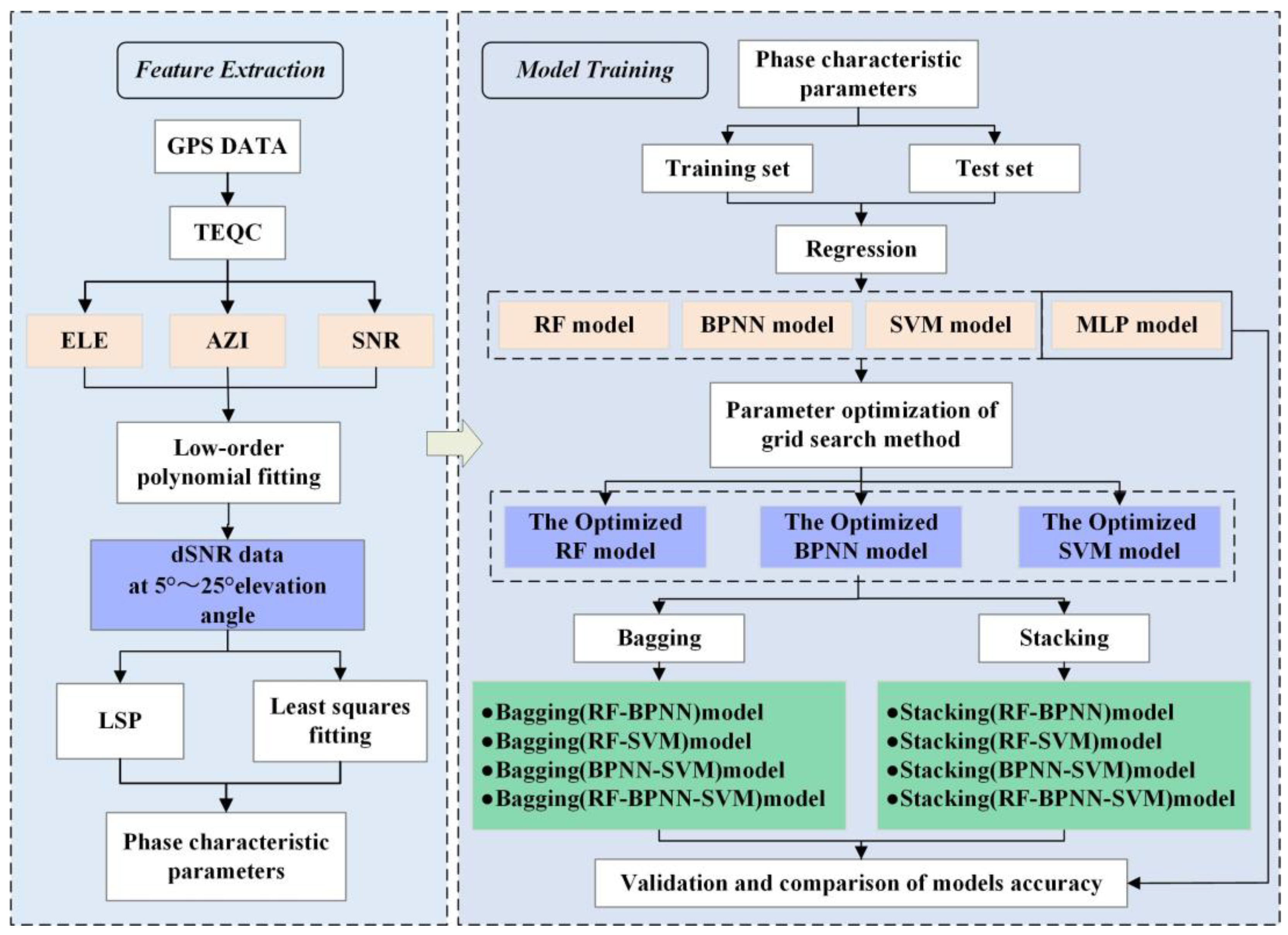
Figure 1. Technical flow chart.
Land 14 01716 g001
Figure 2. The GNSS-IR observation schematic illustrates that h represents the vertical distance from the GNSS antenna to the ground surface, while θ corresponds to the satellite’s elevation angle.
Land 14 01716 g002
Figure 3. Bagging integrated learning algorithm framework diagram.
Land 14 01716 g003
Figure 4. Stacking an integrated learning algorithm framework diagram.
Land 14 01716 g004
Figure 5. Overview of the study area and map of the site surroundings.
Land 14 01716 g005
Figure 6. Comparison of rainfall and soil moisture at stations P039, P041, and P043.
Land 14 01716 g006
Figure 7. Comparison of soil moisture retrieval results with reference data for each base model at stations P039, P041, and P043.
Land 14 01716 g007
Figure 8. Comparison between the soil moisture retrieval results from each ensemble learning model and the reference data at station P039.
Land 14 01716 g008
Figure 9. Comparison between the soil moisture retrieval results from each ensemble learning model and the reference data at station P041.
Land 14 01716 g009
Figure 10. Comparison between the soil moisture retrieval results from each ensemble learning model and the reference data at station P043.
Land 14 01716 g010
Figure 11. Scatter plot of soil moisture content inversion results from each reference model and reference values.
Land 14 01716 g011
Figure 12. Scatter plot of inversion results from various integrated models and reference values at Station P039.
Land 14 01716 g012
Figure 13. Scatter plot of inversion results from various integrated models and reference values at Station P041.
Land 14 01716 g013
Table 1. Plot of optimal parameters for each base model.
ModelsOptimization MethodsHyper-ParametersOptimal Parameters
BPNNGrid search methodepochs1500
goal1 × 10−6
lr0.005
RFGrid search methodtrees300
leaf3
Split CriterionMSE
SVMGrid search methodKernel FunctionRBF
Kernel Scale0.4
Box Constraint1
Layer1Size123
MLPGrid search methodLayer2Size124
Initial Learn Rate1 × 10−4
L2Regularization6 × 10−4
Table 2. R, RMSE, and MAE between all model retrieval results and reference values.
StationModelRRMSE
cm3/cm3
MAE
cm3/cm3
P039BPNN0.7870.05880.0449
RF0.8810.05010.0421
SVM0.8390.0510.0421
MLP0.8790.0450.0384
(Bagging) BPNN-RF0.8630.04840.0383
(Bagging) BPNN-SVM0.8350.0510.0397
(Bagging) RF-SVM0.8760.04860.0408
(Bagging) BPNN-RF-SVM0.8670.04790.0386
(Stacking) BPNN-RF0.8910.04840.0417
(Stacking) BPNN-SVM0.8310.05180.0439
(Stacking) RF-SVM0.8890.04520.0378
(Stacking) BPNN-RF-SVM0.9030.04460.0371
P041BPNN0.8230.06830.0547
RF0.8760.05980.0409
SVM0.860.0610.0441
MLP0.880.0550.041
(Bagging) BPNN-RF0.8740.0580.0435
(Bagging) BPNN-SVM0.8610.05990.0465
(Bagging) RF-SVM0.8810.05820.0402
(Bagging) BPNN-RF-SVM0.8790.05720.0424
(Stacking) BPNN-RF0.8760.05980.0411
(Stacking) BPNN-SVM0.8660.05980.0436
(Stacking) RF-SVM0.8860.05720.0395
(Stacking) BPNN-RF-SVM0.9040.05220.0379
P043BPNN0.8460.07170.0577
RF0.8960.06210.0529
SVM0.870.06430.0534
MLP0.8920.05760.0462
(Bagging) BPNN-RF0.8960.05770.0469
(Bagging) BPNN-SVM0.8850.05960.0481
(Bagging) RF-SVM0.8960.06130.0526
(Bagging) BPNN-RF-SVM0.9020.05720.0467
(Stacking) BPNN-RF0.9010.06080.0509
(Stacking) BPNN-SVM0.8760.0630.0524
(Stacking) RF-SVM0.9050.05770.0483
(Stacking) BPNN-RF-SVM0.9170.05450.0457
Disclaimer/Publisher’s Note: The statements, opinions and data contained in all publications are solely those of the individual author(s) and contributor(s) and not of MDPI and/or the editor(s). MDPI and/or the editor(s) disclaim responsibility for any injury to people or property resulting from any ideas, methods, instructions or products referred to in the content.