Spatial Distribution of Grain Yield in the Songnen Plain Agro-Pastoral Zone in Heilongjiang Province: A Study Using Geostatistics and Geographically Weighted Regression

Abstract

This study examines the spatial distribution of grain yield in the Songnen Plain Agro-Pastoral Zone in Heilongjiang Province from 2015, 2017, 2019 and 2021, using Kriging interpolation as the primary method. Ordinary Kriging (exponential kernel/semivariogram, step = 13) achieved optimal accuracy (RMSE = 0.856), outperforming Co-Kriging. Incorporating all covariates lowered precision due to weak spatial autocorrelation in slope and aspect, while limiting covariates to elevation and soil type improved results. Spatial patterns revealed a southwest-to-northeast gradient. Over time, yields increased notably in the southwest and northern areas, with Wudalianchi rising by 259.71%, but declining locally, such as a 12.20% drop in Shuangcheng. Environmental factors like slope and soil showed spatially heterogeneous influences, interacting with policies and socioeconomic variables. The grain yield center shifted slightly northward. Geographically Weighted Regression (GWR) further validated these spatial patterns. These findings provide valuable insights into covariate selection and spatial drivers, supporting more precise agricultural planning and management in the region.

1. Introduction

The spatial distribution of grain yield is a critical factor influencing agricultural production strategies, resource allocation, and food security [1]. Understanding these spatial patterns enables policymakers and agricultural stakeholders to optimize land use, tailor farming practices to local conditions, and implement targeted interventions to enhance productivity [2,3,4].

Grain yield is intricately influenced by a combination of environmental and land management factors. Topographic attributes such as slope, elevation, and aspect significantly affect soil moisture retention, erosion susceptibility, and solar radiation exposure, thereby impacting crop growth and productivity [5,6,7,8]. For instance, steeper slopes often lead to increased runoff and soil erosion, reducing soil fertility and water availability [9]. Elevation influences temperature and precipitation patterns, which are critical for crop development [10]. Aspect determines the amount of sunlight received, affecting soil temperature and evapotranspiration rates [11,12,13]. Soil types, defined by their texture, structure, and chemical properties, determine water-holding capacity and nutrient supply, directly influencing crop performance [14,15,16].

The Songnen Plain, located in northeastern China, presents a unique agro-pastoral landscape characterized by diverse topography and soil types. This region exhibits complex terrain and soil characteristics, making it an ideal case for studying the spatial variability of grain yield in agro-pastoral landscapes. It also faces environmental challenges such as soil degradation and yield instability, which require spatially informed agricultural planning [17,18,19]. Studying this area provides an opportunity to understand how topographic and land management factors interact to influence grain yield. Insights gained can inform sustainable agricultural practices and land-use planning in similar agro-ecological zones.

Many studies in the Songnen Plain have primarily relied on conventional statistical methods such as Ordinary Least Squares (OLS) regression, multiple linear regression, and correlation analysis to examine agricultural patterns [20,21,22,23]. These methods generally assume spatial stationarity, meaning that relationships between variables are consistent across space. However, in heterogeneous landscapes like the Songnen Plain—characterized by varied topography, soil types, and land-use histories—this assumption is rarely valid. As a result, conventional techniques often fail to capture localized variations and spatial heterogeneity, which are critical for understanding grain yield dynamics [24]. This limitation may obscure important site-specific influences of environmental and topographic factors on yield, particularly in complex Agro-Pastoral zones. To address these limitations, this study integrates Co-Kriging interpolation and Geographically Weighted Regression (GWR) to analyze both the spatial distribution and location-specific drivers of grain yield. While Kriging techniques leverage spatial autocorrelation to estimate values in unsampled areas, GWR allows regression coefficients to vary across space, revealing localized relationships between yield and environmental variables. This combined approach has not yet been systematically applied to the Songnen Plain, and it enables a more nuanced understanding of spatial patterns and driving mechanisms than traditional models. The insights gained can inform more targeted land-use planning and precision agriculture strategies in spatially diverse agricultural regions [25,26].

In response to the limitations of conventional spatial analyses, this study integrates Co-Kriging interpolation and Geographically Weighted Regression (GWR) to more effectively capture the spatial heterogeneity of grain yield in the Songnen Plain Agro-Pastoral Zone in Heilongjiang Province. Co-Kriging enhances yield estimation at unsampled locations by incorporating spatial autocorrelation along with auxiliary topographic variables such as slope and aspect. GWR, meanwhile, is employed to uncover spatially varying relationships between grain yield and environmental factors by allowing model parameters to differ across geographic locations [20]. This dual-method approach is novel in its application to the Songnen Plain and offers a comprehensive framework that not only predicts spatial yield patterns but also reveals localized drivers of variation—an advancement over previous studies that relied on spatially invariant models. The combined use of Co-Kriging and GWR, thus provides improved methodological support for precision agriculture and targeted land-use planning in complex agro-ecological regions.

2. Materials and Methods

2.1. Study Area

The Songnen Plain Agro-Pastoral Zone in Heilongjiang Province is situated in northeastern China, between 44.06° and 51.01° N and 123.05° and 128.484° E, with a total land area of approximately 15.63 million hectares. It encompasses the municipalities of Qiqihar, Daqing, Suihua, the southwestern part of Heihe, and the western part of Harbin [21].

The topography of the region is predominantly flat, and it is characterized by fertile black soils with deep humus layers and high organic matter content. These soil properties provide strong water retention and nutrient-holding capacity, offering highly favorable conditions for agricultural development [22]. The region experiences a cold temperate continental monsoon climate, with cold, dry winters and cool, humid summers. The annual precipitation ranges from 400 mm to 600 mm, concentrated mainly during the growing season, which aligns well with the water needs of major crops [23].

The Songnen Plain is one of China’s most important grain-producing regions, with maize, soybean, wheat, and rice as the primary cultivated crops. In this study, the Songnen Plain Agro-Pastoral Zone in Heilongjiang Province, excluding urban districts where agricultural activities are limited, was selected as the primary study area [24,25,26]. Urban areas were excluded because their limited agricultural activity could introduce significant bias and variability into the analysis, potentially skewing the results. Figure 1 shows the regional overview of the Songnen Plain Agro-Pastoral Zone in Heilongjiang Province [27].

2.2. Research Data

2.2.1. Data Source

The administrative vector data for 35 counties and districts in the Songnen Plain Agro-Pastoral Zone in Heilongjiang Province were sourced from the Tianditu platform (https://www.tianditu.gov.cn/, accessed on 13 July 2025), a national geospatial service that offers reliable mapping data for spatial analysis and planning applications.

County-level statistical data on grain yield and sown area were obtained from the National Bureau of Statistics Yearbooks (https://www.stats.gov.cn/sj/ndsj/, accessed on 13 July 2025), which are widely used as a standard reference for socio-economic and agricultural statistics in China. Although more detailed socio-economic variables (e.g., farm management practices, labor input, and policy subsidies) are also important determinants of grain yield, such data are currently difficult to obtain at consistent spatial and temporal resolutions. This study thus incorporates available yield and sown area statistics as a proxy to reflect some socio-economic characteristics at the regional level.

Topographic data were based on a 30 m resolution Digital Elevation Model (DEM), which was obtained from the United States Geological Survey (USGS) Global Visualization Viewer (GloVis) platform (https://glovis.usgs.gov/, accessed on 13 July 2025). Slope and aspect were subsequently derived through surface analysis of the DEM using ArcGIS (version 10.8) software.

Soil type data were obtained from the Resource and Environment Science and Data Platform (https://www.resdc.cn/Default.aspx, accessed on 13 July 2025), a comprehensive data source supporting research in environmental sciences and land resource management.

The detailed sources and their applications are summarized in

Table 1. Data acquisition for explanatory variables.

Data Source	Data Type	Data Usage
Tianditu Platform (https://www.tianditu.gov.cn/, accessed on 13 July 2025)	Administrative vector data for 35 counties/districts in Heilongjiang’s Agro-Pastoral Zone	Spatial analysis and planning applications
National Bureau of Statistics Yearbooks (https://www.stats.gov.cn/sj/ndsj/, accessed on 13 July 2025)	County-level grain yield and sown area statistics	Standard reference for socio-economic and agricultural statistics in China
USGS GloVis Platform (https://glovis.usgs.gov/, accessed on 13 July 2025)	30 m resolution DEM; Derived slope and aspect (via ArcGIS 10.8 surface analysis)	Topographic analysis
Resource and Environment Science and Data Platform (https://www.resdc.cn/, accessed on 13 July 2025)	Soil type data	Environmental science research and land resource management studies

.

2.2.2. Data Processing

The administrative boundary vector data were clipped to match the spatial extent of the Songnen Plain Agro-Pastoral Zone in Heilongjiang Province (excluding urban areas). To ensure spatial consistency and minimize distortion in regional-scale spatial analyses, the data were reprojected using the Gauss–Kruger coordinate system with a central meridian of 128° E.

Evaluating a region’s grain production solely based on total output is not scientifically robust, as it fails to account for differences in the cultivated area; therefore, in this study, grain yield per unit of sown area (i.e., yield density) was used to more accurately assess the grain yield capacity of each county unit. Yield density was calculated by dividing the total grain yield by the total sown area within each county, with results expressed in tons per square kilometer (t/ha), providing a standardized metric for the spatial comparison of agricultural productivity. This yield density metric helps reduce bias introduced by variations in land size and partially accounts for differences in land-use efficiency across counties. However, other socio-economic and land management variables (e.g., irrigation intensity, fertilizer use, and mechanization) were not included due to the lack of spatially detailed and consistent data. We acknowledge this limitation and highlight the need for future studies to integrate these factors for a more comprehensive explanation of grain yield variability.

Prior to analysis, yield density data underwent outlier detection using the interquartile range (IQR) method, where values beyond 1.5×IQR from the lower or upper quartile were flagged as potential anomalies. Each flagged value was cross-checked against local statistical yearbooks, and anomalies confirmed to result from data entry errors, reporting inconsistencies, or missing records were replaced using inverse distance weighting (IDW) interpolation based on neighboring county values for the corresponding year. IDW leverages spatial autocorrelation to generate plausible estimates for missing or erroneous data, ensuring local spatial patterns are preserved and reducing the influence of spurious extremes [28].

Finally, to meet the statistical assumptions of subsequent interpolation and regression models, grain yield density was transformed using the Box–Cox transformation, which stabilizes variance and improves the normality of residuals, thereby enhancing model fit and reducing bias in spatial predictions [29].

Slope and aspect were extracted using the Surface Analysis tools within the Spatial Analyst extension of ArcGIS (version 10.8). To facilitate the analysis of terrain-related driving factors, the resulting raster layers were reclassified into discrete categories using the Reclassify function. Each category was assigned to a corresponding value based on topographic characteristics, enabling standardized inputs for subsequent spatial modeling and correlation analysis.

The slope classification (assigned values −4 to +4) reflects increasing deviation from optimal cultivation terrain. Moderate slopes (6–15°) are considered the most suitable for grain cultivation, whereas steeper slopes (>25°) are prone to erosion, reduced water retention, and lower mechanization potential. Very flat areas ([0, 2]°) may present drainage challenges and were accordingly weighted negatively. Aspect categories were assigned ordinal scores based on sunlight exposure and microclimate influence. In the Northern Hemisphere, south- and southeast-facing slopes generally offered favorable thermal and moisture conditions for crops. Flat areas (aspect = −1) received the lowest score, and continuity was maintained by assigning similar values to both the [0–22.5]° and [337.5–360]° bins [30]. Soil type values were assigned based on fertility ranking with the highest values for Black Soil and Chernozem—both rich in organic matter and key to agricultural productivity in Northeast China—and progressively lower values for meadow-based or swampy soils reflecting diminishing fertility [31,32]. In this study, land quality and cultivated land suitability grading were based on the FAO Framework for Land Evaluation (FAO, 1976) and current Chinese cultivated land quality grading guidelines. A semi-quantitative scoring method was applied, integrating factors such as terrain, soil, and crop adaptability. The specific grading criteria were developed in accordance with agricultural production practices and relevant policy documents, ensuring that the classification results were scientifically sound and aligned with regional agricultural development realities [33].

A uniform-interval (arithmetic-sequence) value assignment was adopted (e.g., 2-point increments for slope/aspect; 0.5–1.0 increments for soil types). This approach preserves ordinal relationships without implying precise numeric ratios, minimizes subjective bias, and supports model integration (e.g., GWR, Co-Kriging), as commonly applied in land-suitability and agro-ecological zoning studies [31,34]. This semi-quantitative scoring method enables meaningful representation of terrain and soil influences in spatial models while maintaining transparency and reproducibility, details are shown in

Table 2. The reclassification and value assignment criteria for slope, aspect, and soil type.

Category	Range/Type	Assigned Value
Slope (°)	[0, 2]	−4
	(2, 6)	−2
	(6, 15)	0
	(15, 25)	2
	[25, 90]	4
Aspect (°)	−1 (Flat area)	1
	[0, 22.5]	2
	(22.5, 67.5]	3
	(67.5, 112.5]	4
	(112.5, 157.5]	5
	(157.5, 202.5]	6
	(202.5, 247.5]	7
	(247.5, 292.5]	8
	(292.5, 337.5]	9
	(337.5, 360]	2
Soil Type	Black Soil	9.5
	Chernozem	8.5
	Meadow Black Soil	8
	Meadow Soil	7.5
	Meadow Black Calcium	7
	Calcareous Grass	6
	Dark Brown Soil	5.5
	Lime Black	5
	Meadow Sandstorm	4
	Swampy Soil	3

.

2.3. Methodology Overview

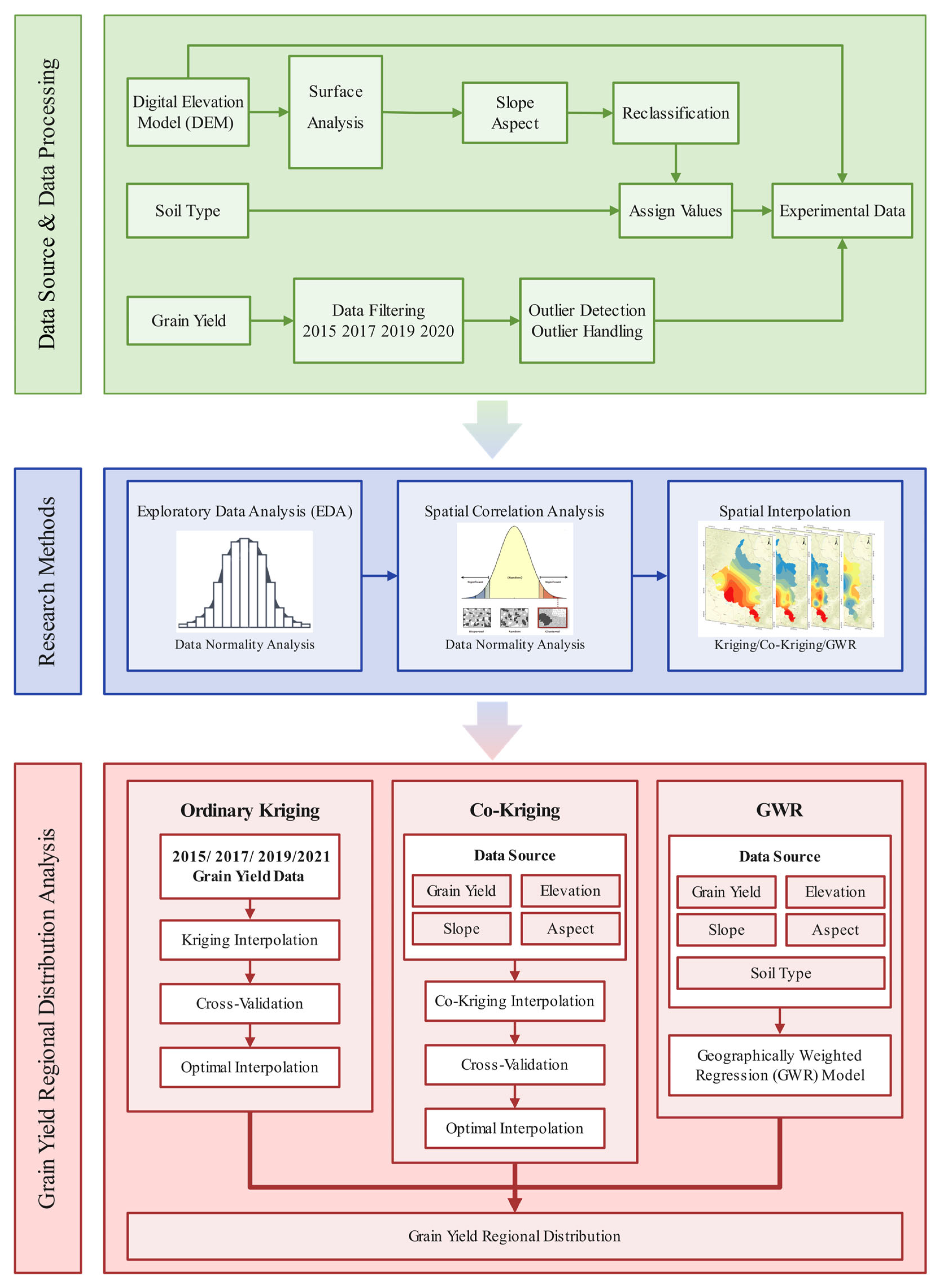
Firstly, driving factors such as elevation and slope were preprocessed and reclassified with assigned values to facilitate subsequent spatial analysis. Then, Exploratory Data Analysis (EDA) was conducted, including the calculation of both Global and Local Moran’s I, to investigate spatial autocorrelation and clustering patterns in grain yield distribution. Subsequently, Ordinary Kriging and Co-Kriging (incorporating elevation, slope, and aspect as covariates) were used for spatial interpolation. The optimal interpolation method was selected based on cross-validation results. Finally, Geographically Weighted Regression (GWR) was applied to further validate and explore the spatial relationship between grain yield and terrain-related factors. The overall methodology framework is illustrated in Figure 2.

2.4. Research Methods

2.4.1. Exploratory Data Analysis (EDA)

(1)

Histogram (Distribution Assessment)

Histograms were used to examine the frequency distribution of grain yield and its associated variables [35,36]. A histogram partitions the data into a series of bins (intervals), with the height of each bar representing the number of observations $f_k$ falling into bin $k$. The general form of a histogram density estimate is given by:

$$f\left(x\right)={\displaystyle \frac{1}{nh}}\sum _{i=1}^{n}1\left({\displaystyle \frac{\mathit{x}-{\mathit{x}}_{\mathit{i}}}{\mathit{h}}}\in [{\mathit{a}}_{\mathit{k}},{\mathit{a}}_{\mathit{k}+1})\right)$$

(1)

where $n$ is the total number of observations, $h$ is the bin width, $x_i$ is the $i$-th observation, and $1(·)$ is the indicator function that equals 1 if the condition is true and 0 otherwise. The histogram provides a visual assessment of skewness, kurtosis, and modality, which supports data preprocessing and transformation decisions.

(2)

Q–Q Plot (Normality Check)

To assess whether the data follow a normal distribution, Quantile–Quantile (Q–Q) plots were constructed [37,38,39]. (Q–Q) plots compare the empirical quantiles of a variable a with the corresponding theoretical quantiles $z_i$ from a standard normal distribution:

$$z_i={\mathit{\Phi }}^{-1}\left({\displaystyle \frac{i-0.5}{n}}\right)$$

(2)

where ${\mathit{\Phi }}^{-1}$ is the inverse cumulative distribution function (CDF) of the standard normal distribution, $i$ denotes the rank in ascending order, and $n$ is the total number of observations. If the plotted points fall approximately along the 45° line, the data are considered normally distributed.

(3)

Box–Cox Transformation (Normalization Adjustment)

To improve the normality of grain yield data prior to regression analysis, a Box–Cox transformation was applied. The transformation parameter ($\lambda$) was selected based on the skewness and kurtosis of the distribution. Skewness measures the asymmetry of a distribution, with a value of zero indicating perfect symmetry, while kurtosis quantifies the “peakedness” or heaviness of the tails; a kurtosis of 3 typically represents a normal distribution. In this study, a series of $\lambda$ values were tested and evaluated. When $\lambda$ = 1.32, the yield distribution exhibited optimal skewness (0.0013) and kurtosis (2.3628), which together indicated the closest approximation to a normal distribution. This provided the justification for choosing $\lambda$ = 1.32 as the optimal Box–Cox transformation parameter.

2.4.2. Spatial Correlation Analysis

(1)

Global Moran’s I (Spatial Autocorrelation)

Global Moran’s I statistic was used to quantify the degree of overall spatial autocorrelation of grain yield across all counties [40]. It is defined as:

$$I={\displaystyle \frac{n}{W}}\cdot {\displaystyle \frac{{\sum }_{i=1}^n{\sum }_{j=1}^n{w}_{ij}\left(x_i-\overline{x}\right)\left(x_j-\overline{x}\right)}{{\sum }_{i=1}^n{\left(x_i-\overline{x}\right)}^2}}$$

(3)

where $x_i$ and $x_j$ represent the observed values at locations $i$ and $j$, $\overline{x}$ is the global mean, $w_{ij}$ is the spatial weight between units $i$ and $j$, $W={\sum }_i{\sum }_j{w}_{ij}$ is the sum of all spatial weights, and $n$ is the number of spatial units. A positive Moran’s I indicates clustering of similar values, while a negative value suggests spatial dispersion.

(2)

Local Moran’s I (LISA)

Local spatial clustering patterns were further analyzed using Local Indicators of Spatial Association (LISA), specifically the Local Moran’s I statistic for each spatial unit $i$:

$$I_i=\left(x_i-\overline{x}\right)\sum _{j=1}^n{w}_{ij}\left(x_j-\overline{x}\right)$$

(4)

where $x_i$ is the observed value at unit $i$, $\overline{x}$ is the mean of all observations, and $w_{ij}$ is the spatial weight between unit $i$ and its neighboring unit $j$. The sign and magnitude of $I_i$ indicate the presence and type of local spatial association, such as high-high (HH), low-low (LL), high-low (HL), and low-high (LH) clusters [41].

2.4.3. Kriging Interpolation

(1)

Ordinary Kriging Interpolation

Ordinary Kriging is a widely used geostatistical interpolation method that estimates the value of a variable at unsampled locations based on spatial autocorrelation among known data points [42]. As a form of univariate interpolation, it assumes that the mean of the underlying process is unknown but constant within the local neighborhood [43,44].

The prediction at an unsampled location $x_0$ is obtained as a weighted linear combination of the observed values $z\left(x_i\right)$:

$$\widehat{z}(x_0)=\sum _{i=1}^n{\lambda }_{i}z\left(x_i\right)$$

(5)

Subject to the unbiasedness condition:

$$\sum _{i=1}^n{\lambda }_i=1$$

(6)

where ${\lambda }_i$ are the kriging weights assigned to each observed point $x_i$, determined by solving the Ordinary Kriging system based on the semivariogram model.

The semivariogram $\gamma \left(h\right)$, which quantifies spatial dependence as a function of lag distance $h$, is defined as:

$$\gamma \left(h\right)={\displaystyle \frac{1}{2N\left(h\right)}}\sum _{i=1}^{N\left(h\right)}{\left[z\left(x_i\right)-z(x_i+h)\right]}^2$$

(7)

where $N\left(h\right)$ is the number of data pairs separated by distance $h$. A theoretical semivariogram model is fitted to empirical data and used to estimate kriging weights.

(2)

Co-Kriging Interpolation

Co-Kriging is an advanced multivariate geostatistical interpolation method that extends the kriging framework by incorporating one or more auxiliary variables that are spatially correlated with the primary variable of interest [45,46]. By leveraging the covariation between variables, Co-Kriging improves prediction accuracy in situations where the primary variable is sparsely sampled or exhibits strong spatial heterogeneity [47].

The Co-Kriging estimate at an unsampled location $x_0$ is defined as:

$$\widehat{z}\left(x_0\right)=\sum _{i=1}^n{\lambda }_{i}z\left(x_i\right)+\sum _{j=1}^m{\mu }_j{y}_j\left(x_j\right)$$

(8)

where $z\left(x_i\right)$ is the primary variable (e.g., grain yield), $y_j$ are the secondary variables (e.g., elevation, slope, and aspect), and ${\lambda }_i$, ${\mu }_j$ are the kriging weights determined by solving a Co-Kriging system based on auto- and cross-variograms.

2.4.4. Cross-Validation

To evaluate the performance and reliability of spatial interpolation methods, a leave-one-out cross-validation approach was applied [48,49,50]. The predictive accuracy was assessed using five standard statistical metrics: Mean Error (ME), Root Mean Squared Error (RMSE), Mean Squared Error (MSE), Root Mean Squared Standardized Error (RMSSE), and Average Standard Error (ASE). These indicators provide comprehensive insights into both the bias and precision of the interpolation results [51,52].

$$\mathrm{M}\mathrm{E}={\displaystyle \frac{1}{n}}\sum _{i=1}^n\left({\widehat{z}}_i-z_i\right)$$

(9)

$$\mathrm{R}\mathrm{M}\mathrm{S}\mathrm{E}=\sqrt{{\displaystyle \frac{1}{n}}\sum _{i=1}^n{\left({\widehat{z}}_i-z_i\right)}^2}$$

(10)

$$\mathrm{M}\mathrm{S}\mathrm{E}={\displaystyle \frac{1}{n}}\sum _{i=1}^n{\left({\widehat{z}}_i-z_i\right)}^2$$

(11)

$$\mathrm{R}\mathrm{M}\mathrm{S}\mathrm{S}\mathrm{E}=\sqrt{{\displaystyle \frac{1}{n}}\sum _{i=1}^n{\left({\displaystyle \frac{{\widehat{z}}_i-z_i}{{\sigma }_i}}\right)}^2}$$

(12)

$$\mathrm{A}\mathrm{S}\mathrm{E}={\displaystyle \frac{1}{n}}\sum _{i=1}^n{\sigma }_i$$

(13)

where ${\widehat{z}}_i$ denotes the predicted value, $z_i$ is the observed value, ${\sigma }_i$ is the kriging standard error, and $n$ is the number of validation samples.

2.4.5. Geographically Weighted Regression (GWR)

Geographically Weighted Regression (GWR) is a local spatial regression technique designed to model spatial heterogeneity by allowing regression coefficients to vary across geographic locations [53,54,55]. Unlike global regression models, which assume spatial stationarity, GWR captures local variations in relationships between the dependent and independent variables [56].

The GWR model at a location $i$ is expressed as:

$$y_i={\beta }_0\left(u_i,v_i\right)+\sum _{k=1}^P{\beta }_k\left(u_i,v_i\right)x_{ik}+{\epsilon }_i$$

(14)

where $\left(u_i,v_i\right)$ are the coordinates of the location $i$, $x_{ik}$ are the explanatory variables, ${\beta }_k\left(u_i,v_i\right)$ are location-specific regression coefficients, and ${\epsilon }_i$ is the error term.

3. Results

3.1. Distributional Characteristics of Grain Yield

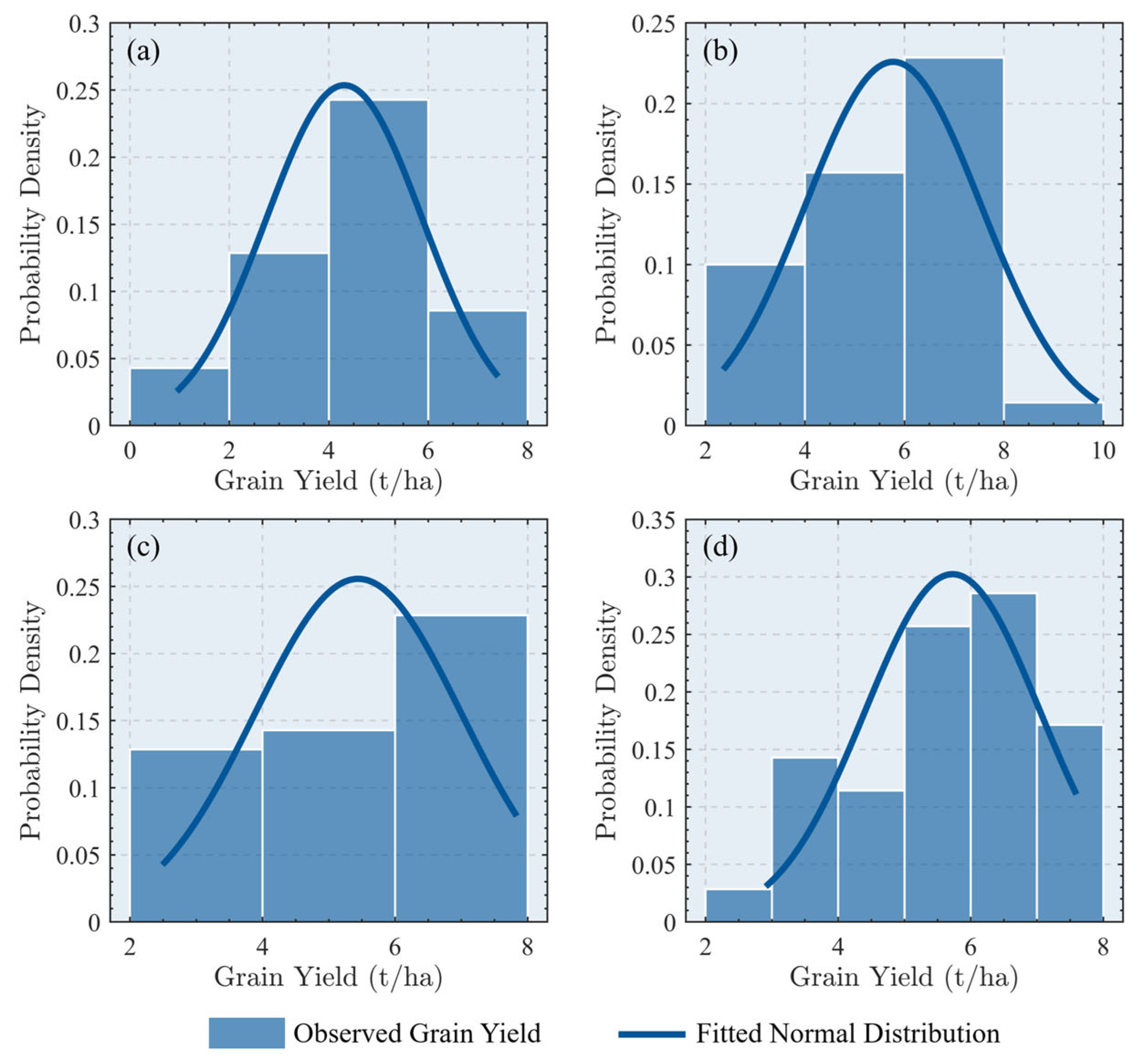
The county-level grain yield data in the Songnen Plain exhibited a noticeably skewed distribution, deviating from the assumptions of normality required for parametric spatial analyses. To reduce skewness and improve distributional symmetry, a Box–Cox transformation was applied with an optimal parameter of $\lambda$ = 1.32. The transformed data showed a more symmetrical, bell-shaped distribution, approximating normality and providing a more suitable input for subsequent spatial statistical methods, as shown in Figure 3.

To further evaluate the normality of the transformed grain yield data, Q–Q (quantile–quantile) plots were employed. This visual diagnostic tool compares the quantiles of the observed data with those of a theoretical normal distribution. Following the Box–Cox transformation ($\lambda$ = 1.32), the Q–Q plot showed a marked improvement in alignment with the theoretical quantile line. The overall distribution became significantly more consistent with the assumptions of normality, as shown in Figure 4.

3.2. Spatial Distribution of Grain Yield

3.2.1. Spatial Autocorrelation Assessment via Global Moran’s I

Global Moran’s I is an important index for measuring spatial autocorrelation in spatial data, used to assess the spatial distribution pattern of similar values within a study area. By calculating the Moran’s I, it is possible to determine the clustering or dispersion trend of a variable in space. The calculation of Moran’s I involves several key parameters, each providing valuable insights into the spatial autocorrelation of the data.

The calculation of Moran’s I involves several key parameters that provide valuable insights into spatial autocorrelation. Moran’s I itself reflects the strength of spatial autocorrelation and ranges from −1 to +1. Positive values indicate spatial clustering, where similar values tend to group together, while negative values suggest spatial dispersion, where similar values are spread out; values close to zero imply a random spatial distribution with no significant clustering or dispersion. The z-value is the standardized value of Moran’s I, used to assess the statistical significance of spatial autocorrelation. A z-value greater than 1.96 or less than −1.96 indicates significant spatial autocorrelation, suggesting that the spatial pattern is unlikely to have occurred by chance. If the z-value is close to zero, it suggests that spatial autocorrelation is not significant, implying that the spatial pattern might be random. The p-value tests the significance of Moran’s I. A smaller p-value indicates a more significant spatial autocorrelation. If the p-value is less than 0.05, it indicates significant spatial autocorrelation, suggesting a notable spatial pattern, whether it be clustering or dispersion. Conversely, a p-value greater than or equal to 0.05 implies no significant spatial autocorrelation, indicating that the spatial distribution is likely random.

The variation in parameter ranges and their corresponding meanings are summarized in

Table 3. The range variability of parameters and their corresponding significance.

Parameter	Range	Interpretation
Moran’s I	0~0.1	Near-random spatial distribution with minimal clustering or dispersion.
	0.1~0.3	Weak spatial clustering, with low spatial autocorrelation.
	0.3~0.5	Moderate spatial clustering, noticeable spatial autocorrelation.
	0.5~0.7	Strong spatial clustering, significant spatial autocorrelation.
	0.7~1.0	Very strong spatial clustering, extremely significant spatial autocorrelation.
z	$\left|z\right|>1.96$	Significant spatial autocorrelation
	$\left|z\right|<1.96$	No significant spatial autocorrelation
p	$<$0.05	Significant spatial autocorrelation, clustering or dispersion is evident.
	$\ge$0.05	No significant spatial autocorrelation, likely random distribution.

below.

Continuing from this, the results from the Moran’s I analysis for 2015, 2017, 2019, and 2021 show consistent positive values of Moran’s I across all years, indicating significant spatial clustering. Specifically, the Moran’s I values ranged from 0.501857 in 2019 to 0.743470 in 2021. The highest spatial autocorrelation occurred in 2021, with a Moran’s I of 0.743, indicating a very strong clustering effect in that year. Although the value decreased slightly to 0.501857 in 2019, it still indicated significant clustering, though not as strong as in 2021. The z-values for each year are significantly greater than 1.96, further supporting the statistical significance of the results. In particular, the z-values ranged from 5.1 in 2019 to 7.46 in 2021, confirming that the spatial patterns observed are highly unlikely to have occurred by chance. A z-value greater than 1.96 in all cases suggests that the spatial clustering detected is robust and meaningful. Additionally, the p-values for all years are zero, further reinforcing the conclusion that the spatial autocorrelation observed is not due to random chance. These low p-values strongly support the significance of the findings, ensuring that the observed clustering is not due to random spatial distribution. The results are summarized in

Table 4. Global Moran’s I index values for the years 2015, 2017, 2019, and 2021.

Year	Moran’s I	z	p
2015	0.524044	5.355138	0.000000
2017	0.718746	7.259855	0.000000
2019	0.501857	5.100871	0.000000
2021	0.743470	7.458499	0.000000

.

3.2.2. Identification of Local Spatial Clusters Through LISA

As all calculated Moran’s I values are greater than zero, this indicates that grain yields across the study area exhibit a clear and statistically significant positive spatial autocorrelation. This means that regions with similar yield levels—whether high or low—tend to cluster together geographically, reflecting a structured and non-random spatial distribution. The LISA cluster map provides a more detailed spatial assessment by identifying specific local clusters and determining their statistical significance.

Compared to the Global Moran’s I, which assesses the overall spatial pattern across the entire region, the LISA (Local Indicators of Spatial Association) analysis focuses on local spatial relationships. While the global index reveals the general presence of spatial dependence, the Local Moran’s I detects fine-scale spatial heterogeneity and identifies both clusters and outliers. It classifies local units into four spatial association types—High-High (HH), Low-Low (LL), High-Low (HL), and Low-High (LH)—to illustrate the nature of the relationship between each location and its neighbors.

As shown in Figure 5, the spatial configuration of the four cluster types shows evident regional variation. High-High (HH) clusters are primarily concentrated in Zhaodong City, Lanxi County, Hulan District, and Bayan County, indicating stable high-yield zones with strong positive local associations. Low-Low (LL) clusters are mostly distributed in Nehe City, Keshan County, Kedong County, Wudalianchi City, and Bei’an City, representing areas with persistently low yields and neighboring underperforming regions. Low-High (LH) clusters appear sporadically in Mulan County and Shuangcheng District, reflecting areas of relatively low yields surrounded by more productive neighbors. Conversely, High-Low (HL) clusters are located in Longjiang County and Suiling County, where higher-yield regions are embedded within broader zones of lower productivity. These spatial outliers may be influenced by local variations in agricultural inputs, infrastructure, or socio-economic development.

3.3. Spatial Interpolation of Grain Yield Distributions

3.3.1. Spatial Patterns Estimated by Ordinary Kriging

To assess the spatial heterogeneity of grain yield across the study area, Kriging-based geostatistical interpolation methods were employed. Various forms of Kriging were tested during the interpolation process, among which Ordinary Kriging demonstrated the most stable and reliable performance. In order to validate the precision and effectiveness of the different interpolation strategies, several cross-validation indicators were calculated, including mean error (ME), root mean square error (RMSE), mean square error (MSE), root mean square standardized error (RMSSE), and average standard error (ASE), as summarized in

Table 5. Cross-validation results for Ordinary Kriging Model parameters: kernel function, semivariogram and step length: (a) kernel function, (b) semivariogram, (c) step length.

(a) Kernel Function
Function	ME	RMSE	MSE	RMSSE	ASE
Exponential	0.005276	0.859	0.000260	0.009880	0.936
Gaussian	0.009104	0.938	0.000219	0.014234	0.673
Constant	0.058056	1.081	0.000264	0.012477	0.843
(b) Semivariogram
Function	ME	RMSE	MSE	RMSSE	ASE
Gaussian	0.005276	0.859	0.000260	0.009880	0.936
Exponential	0.003645	0.903	0.000136	0.009698	0.974
Circular	0.004286	0.869	0.000255	0.009928	0.939
Spherical	0.004252	0.871	0.000249	0.009904	0.940
(c) Step Length
Function	ME	RMSE	MSE	RMSSE	ASE
10	0.002462	0.868	0.000183	0.009990	0.932
11	0.008419	0.877	0.000125	0.010040	0.932
12	0.005276	0.859	0.000260	0.009880	0.936
13	0.003183	0.856	0.000231	0.009826	0.937
14	0.013671	0.847	0.000303	0.009763	0.939
15	0.014739	0.850	0.000301	0.009734	0.943
20	0.016089	0.860	0.000302	0.009773	0.947

. These cross-validation metrics are essential for evaluating the accuracy of the interpolation results, where smaller values generally indicate better model performance and higher predictive accuracy.

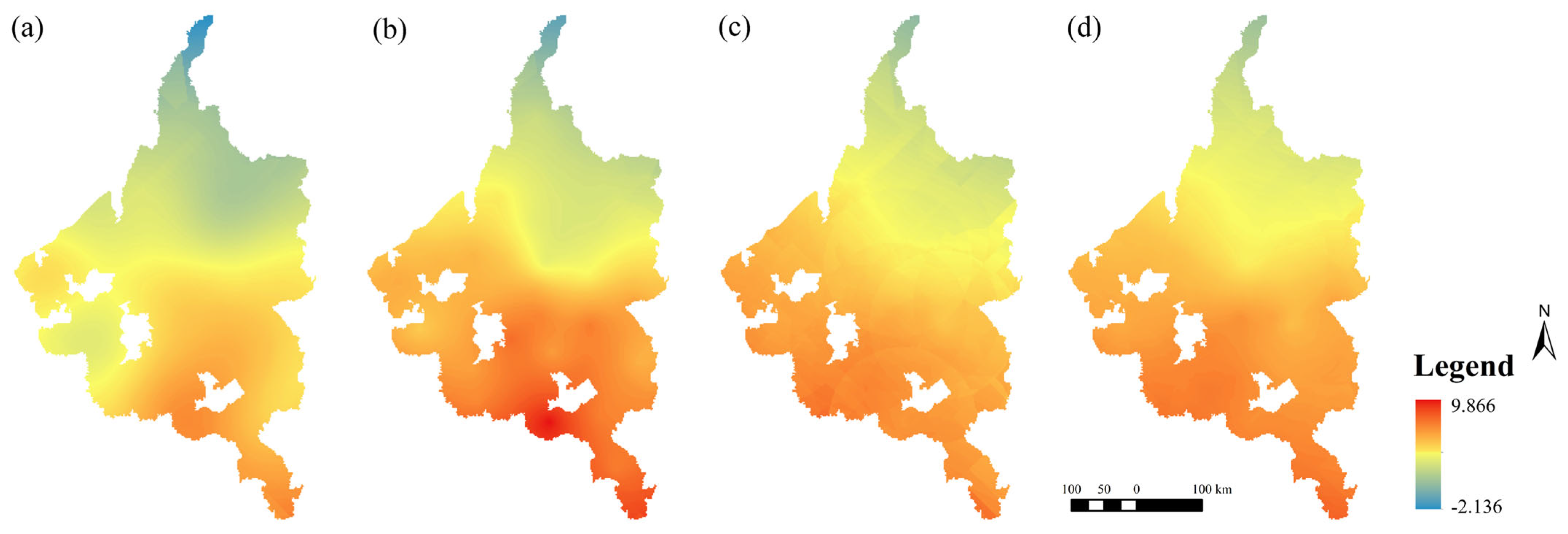
According to the results, the most suitable interpolation performance for grain yield in the Songnen Plain Agro-Pastoral Zone in Heilongjiang Province was achieved when the exponential kernel function, the exponential semivariogram model, and a step length of 13 were used in combination. Ordinary Kriging was demonstrated to be an appropriate and reliable method for analyzing the spatial distribution of grain yield. The resulting interpolation map generated using Ordinary Kriging is shown in Figure 6. Spatially, the interpolated grain yield exhibits a general decreasing gradient from the southwest to the northeast of the study area. Notably, the highest yield during the study period was observed in the Shuangcheng District in 2017. Furthermore, from a temporal perspective, the grain yield across the Songnen Plain demonstrates an overall increasing trend, despite interannual fluctuations.

3.3.2. Co-Kriging-Based Interpolation Incorporating Multiple Data

Co-Kriging interpolation, as an advanced spatial interpolation method, plays a key role in effectively leveraging the spatial correlation between auxiliary variables and the target variable to enhance the accuracy and reliability of interpolation results. Compared with Ordinary Kriging, which relies solely on the spatial distribution information of the target variable itself, Co-Kriging incorporates related auxiliary data, enabling it to better capture subtle spatial variations. This makes it particularly suitable for scenarios where observations of the target variable are sparse or unevenly distributed, significantly reducing interpolation errors and providing more precise foundational data for subsequent spatial analysis and research. In this study, grain yield was selected as the core target variable. Considering the significant impact of natural factors such as topography and soil on grain yield, we incorporated auxiliary variables reflecting topographic features—including elevation, slope, and aspect—as well as soil type to capture differences in soil properties. By integrating these closely related auxiliary variables into the analytical framework, the Co-Kriging interpolation method was applied to perform spatial interpolation across the study area.

Table 6. Cross-validation results for Co-Kriging Model parameters: kernel function, semivariogram and step length: (a) kernel function. (b) semivariogram. (c) step length.

(a) Kernel Function
Function	ME	RMSE	MSE	RMSSE	ASE
Exponential	0.004477	0.895	0.000256	0.010053	0.935
Gaussian	0.027222	0.934	0.000442	0.014390	0.671
Constant	0.031376	1.024	0.000003	0.012051	0.856
(b) Semivariogram
Function	ME	RMSE	MSE	RMSSE	ASE
Gaussian	0.004477	0.895	0.000256	0.010053	0.935
Exponential	0.010440	0.943	0.000152	0.009818	0.975
Circular	0.007622	0.916	0.000200	0.010056	0.947
Spherical	0.005862	0.914	0.000223	0.010020	0.946
(c) Step Length
Function	ME	RMSE	MSE	RMSSE	ASE
10	0.004477	0.895	0.000256	0.010053	0.935
11	0.002328	0.908	0.000218	0.009749	0.963
12	0.017430	0.905	0.000108	0.010157	0.934
13	0.007642	0.891	0.000213	0.009992	0.936
14	0.000808	0.910	0.000243	0.009806	0.962
15	0.013132	0.898	0.000330	0.009689	0.965
20	0.013529	0.899	0.000165	0.010123	0.932

presents the cross-validation results of the Co-Kriging interpolation for the study area, demonstrating the effectiveness and robustness of the method in improving spatial estimation accuracy.

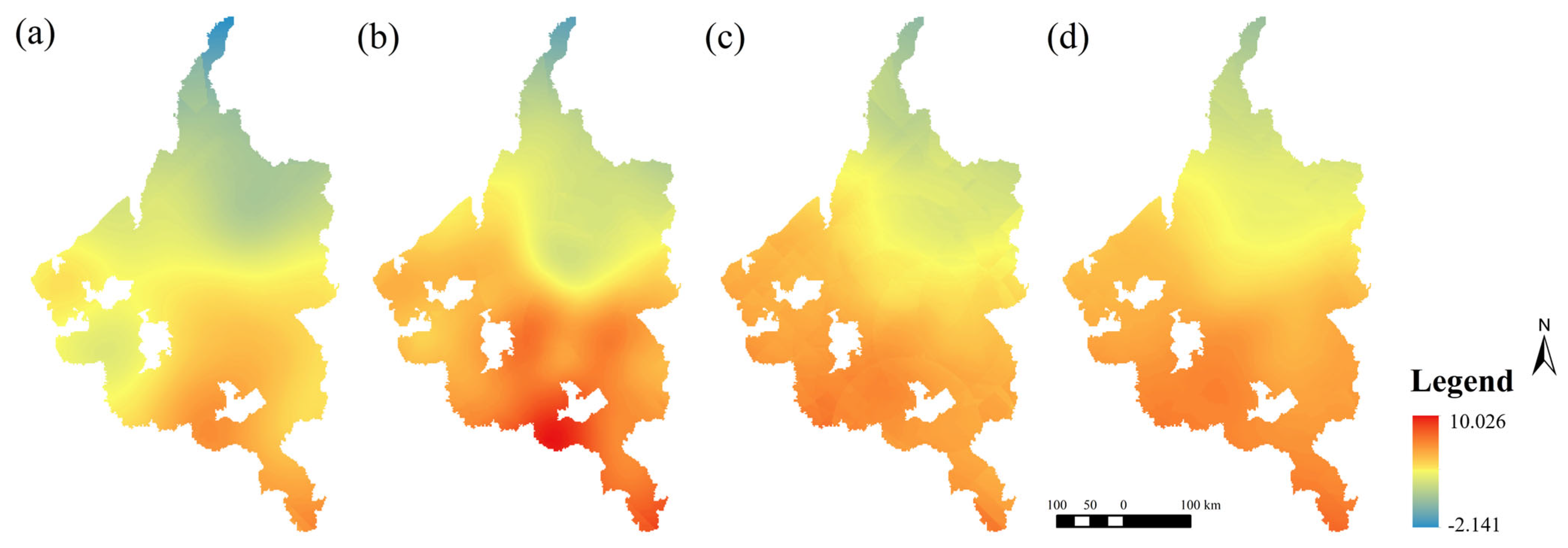
According to the cross-validation results, the optimal Co-Kriging interpolation performance was achieved when the kernel function was set to Exponential, the semivariogram model adopted was Gaussian, and the step length was 13. Under this configuration, the interpolation accuracy was significantly improved, indicating that the selected auxiliary variables contributed effectively to refining the spatial prediction of grain yield. Moreover, a comparative analysis between the Co-Kriging and Ordinary Kriging results reveals a high degree of consistency in the spatial patterns produced by both methods. Specifically, both interpolation approaches exhibit a clear decreasing gradient in grain yield from the southwest to the northeast of the study area, as shown in Figure 7.

3.3.3. Performance Comparison and Optimal Kriging Method

A performance comparison between Ordinary Kriging (OK) and Co-Kriging (CK) was conducted using cross-validation to identify the most effective spatial interpolation approach in this study. Each method was evaluated under various configurations of kernel function, semivariogram model, and step length. The evaluation metrics included Mean Error (ME), indicating the average deviation between predicted and observed values; Root Mean Square Error (RMSE), reflecting the overall magnitude of prediction errors; Mean Squared Error (MSE), providing a squared measure of prediction error; Root Mean Squared Standardized Error (RMSSE), describing the accuracy of standardized residuals; and Average Standard Error (ASE), representing the mean predicted standard deviation. For OK, the optimal configuration was obtained with an Exponential kernel function, an Exponential semivariogram, and a step length of 13, resulting in an RMSE of 0.856, ME of 0.003183, and RMSSE of 0.009826, with ASE closely matching the RMSE. For CK, the best performance was achieved with an Exponential kernel function, a Gaussian semivariogram, and the same step length of 13, resulting in an RMSE of 0.891, ME of 0.004217, and RMSSE of 0.010152. A comparison of these optimal configurations shows that OK produced slightly lower RMSE and ME values than CK in this dataset (Figure 8).

3.4. Validation of Interpolated Patterns via GWR

Geographically Weighted Regression (GWR), as a local regression model that incorporates spatial heterogeneity analysis, is theoretically based on relaxing the traditional global regression assumption of “spatial stationarity of regression coefficients.” By introducing a spatial weighting matrix, GWR constructs location-specific regression equations that allow the relationship between explanatory and dependent variables to vary dynamically across geographic space. This method assigns differentiated weights to sample points based on their spatial location using a kernel function, enabling precise capture of local characteristics and effectively revealing the spatial non-stationarity of variable relationships. As such, GWR provides a quantitative analytical tool for uncovering the mechanisms underlying spatial differentiation in geographic phenomena. In this study, elevation, slope, and aspect were selected as key indicators representing topographic conditions, along with soil type to reflect soil property variability. These factors were integrated to construct a comprehensive set of influencing variables, and the GWR model was applied to quantitatively analyze grain yield across the study area. The results are presented in Figure 9.

The results obtained from the Geographically Weighted Regression (GWR) model are consistent with those derived from both Ordinary Kriging and Co-Kriging interpolation methods, all revealing a clear spatial gradient of decreasing grain yield from the southwest to the northeast across the study area. Moreover, the GWR results align with the Kriging-based approaches not only in terms of the overall spatial trend but also in capturing finer-scale spatial variations. For instance, all methods indicate a pattern of initial increase followed by a subsequent decline in grain yield in the southwestern part of the Songnen Plain, while the northeastern region exhibits a general upward trend. This consistency across methods reinforces the reliability of the identified spatial patterns and highlights the robustness of the influencing factors selected for analysis.

3.5. GWR-Based Spatial Heterogeneity Analysis

To further explore the spatially varying relationships between grain yield and key influencing factors, Geographically Weighted Regression (GWR) was applied to quantify the local effects of these factors across the study area. This section presents the spatial distribution of local regression coefficients, evidence of spatial non-stationarity, and model diagnostic results to validate the robustness of the GWR model.

3.5.1. Model Performance and Residual Diagnostics

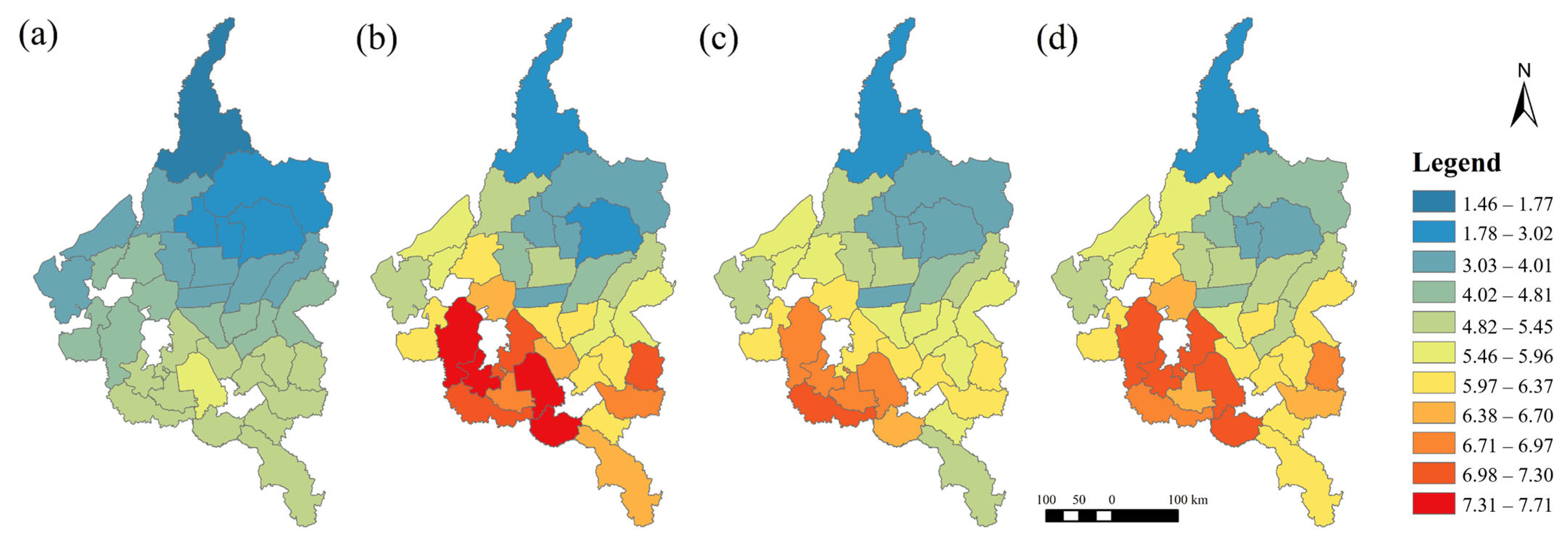
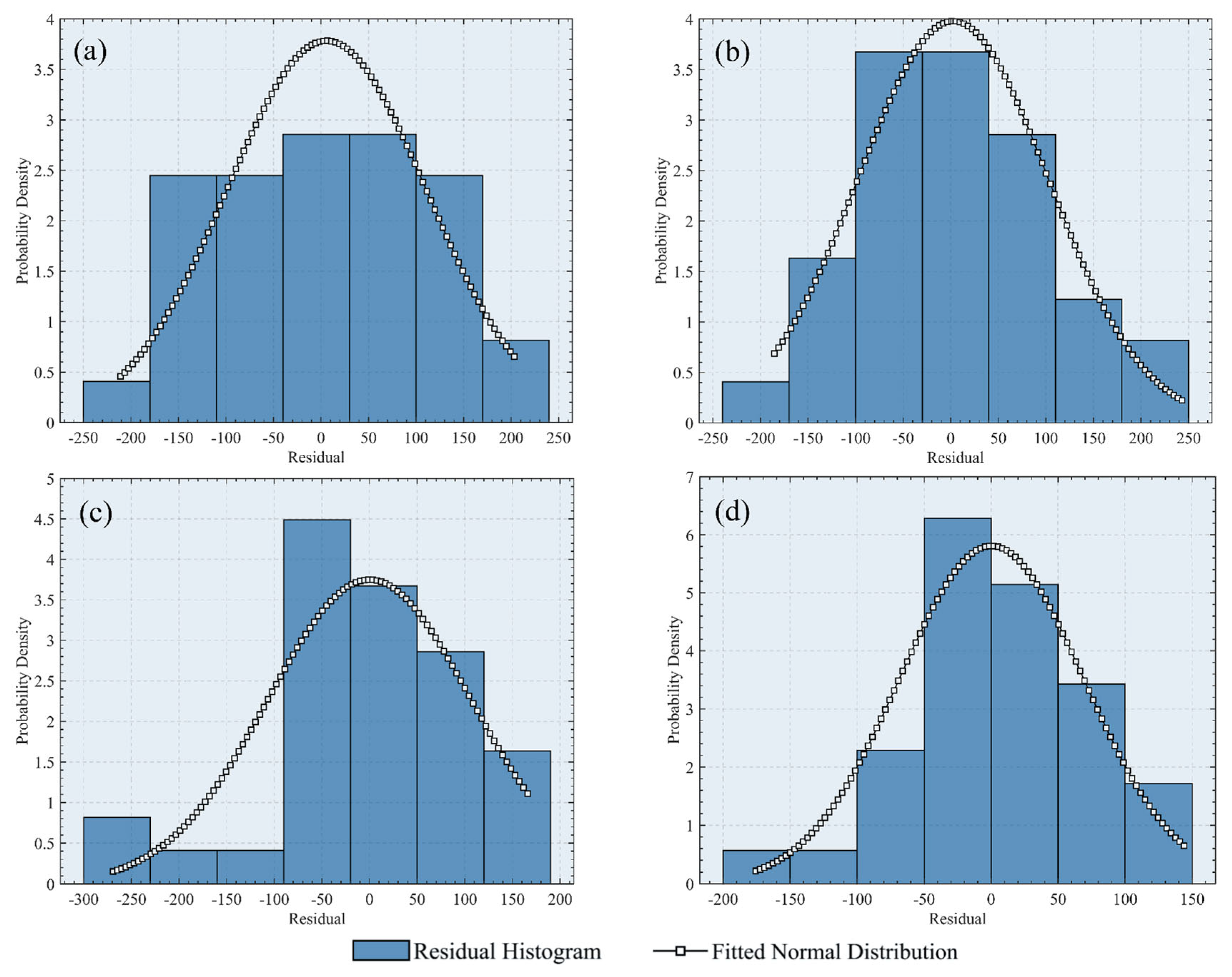
To assess the feasibility and robustness of the GWR model, it is crucial to examine the characteristics of its residuals. Residual analysis helps determine whether the model errors are randomly distributed and conform to the assumptions of normality, which is essential for reliable inference and interpretation of spatial regression results. The Kolmogorov–Smirnov (K–S) and Jarque–Bera (J–B) tests were used to evaluate the normality of GWR residuals across four time points (2015, 2017, 2019, and 2021), and the results indicate that the residuals do not significantly deviate from a normal distribution in any year. Specifically, for 2015, the K–S test returned h = 0, p = 0.9611, and the J–B test yielded h = 0, p = 0.5000; for 2017, h = 0, p = 0.9463 (K–S) and h = 0, p = 0.4264 (J–B); for 2019, h = 0, p = 0.9081 (K–S) and h = 0, p = 0.1503 (J–B); and for 2021, h = 0, p = 0.8901 (K–S) and h = 0, p = 0.5000 (J–B). In all cases, the null hypothesis of normality could not be rejected at the 5% significance level, confirming that the GWR residuals are approximately normally distributed. This suggests that the model is statistically appropriate and that the residuals do not exhibit significant bias or heteroscedasticity. The histogram plots of GWR residuals for 2015, 2017, 2019, and 2021 exhibit distributions that closely approximate a normal curve, further validating the normality assumption of the residuals, as shown in Figure 10.

Compared to the OLS model (R² = 0.3249; Adjusted R² = 0.2595), the GWR model achieved a markedly better explanatory performance (R² = 0.7290; Adjusted R² = 0.6792), further confirming its suitability for modeling spatial heterogeneity in crop yield determinants. To further assess the spatial independence of model residuals, both Global and Local Moran’s I statistics were computed. For the GWR residuals, the Global Moran’s I analysis yielded a z-score of 2.2389 and a p-value of 0.0252, indicating that the observed spatial clustering is unlikely to have occurred by random chance (less than 5% probability). This suggests that although GWR significantly reduces spatial dependence compared to OLS, a modest level of spatial autocorrelation persists. Further analysis using Local Indicators of Spatial Association (LISA) revealed high-high residual clustering in Beilin County and low-low clustering in Nehe City and Dorbod Mongol Aut. County. These results provide a clearer picture of the spatial distribution of residuals and the effectiveness of the GWR model in addressing spatial structure in the data, as shown in Figure 11.

3.5.2. Spatial Heterogeneity of Explanatory Variables: GWR Coefficient Patterns

While the primary purpose of using the GWR model was to validate the spatial patterns identified through Kriging interpolation, its local coefficient estimates also provide valuable insights into the spatial non-stationarity of crop yield determinants. Spatial analysis of the local regression coefficients highlights regional differences in how each environmental factor influences crop yield. This spatially nuanced perspective not only supports the validity of the Kriging results but also deepens the understanding of ecological and agronomic patterns across the study area. Analysis of the local coefficients for the four selected static explanatory variables—slope, aspect, elevation, and soil type—reveals substantial spatial variability in their respective effects on crop yield, further underscoring the non-stationary nature of these relationships. The local regression coefficients for the four static explanatory variables exhibit clear and geographically coherent patterns across the study area. Slope shows a pronounced latitudinal gradient, with negative coefficients concentrated in the southern counties—indicating a weaker or adverse influence on grain yield—and positive coefficients prevailing in the northern counties, where the influence becomes favorable. The lowest values occur in Wuchang City in the south, while the highest positive values are found in Nenjiang City in the north. Aspect coefficients are uniformly positive throughout the region, suggesting a consistently beneficial effect on yield; however, their magnitude increases progressively from the predominantly low-value western counties to the higher-value eastern counties, with the smallest in Wuchang City and the largest in Qing’an County. Elevation exhibits a northeast–southwest gradient, with negative coefficients dominating the northeastern part of the study area and positive coefficients concentrated in the southwestern counties; the lowest values are in Wudalianchi City (northeast), whereas the highest are in Tailai County (southwest). Soil type coefficients increase from east to west, with negative effects concentrated in the eastern counties, particularly Wuchang City, while positive effects are clustered in the western counties, peaking in Tailai County. The spatial distribution of local regression coefficients for the four static explanatory variables—slope, aspect, elevation, and soil type—highlights the geographic variability in their effects on grain yield, as shown in Figure 12.

4. Discussion

4.1. Quantitative Analysis of Covariate Selection and Model Performance in Co-Kriging Interpolation

An unexpected result observed in this study is that the Co-Kriging model incorporating multiple covariates showed lower prediction accuracy (RMSE = 0.891) compared to the ordinary Kriging model based solely on a single variable (RMSE = 0.856). This finding runs counter to the common expectation that including relevant covariates should enhance interpolation performance. To investigate this phenomenon systematically and provide a robust explanation, a quantitative analysis of the spatial properties of potential covariates was conducted prior to the Co-Kriging modeling.

The accuracy of Co-Kriging interpolation fundamentally depends on the spatial autocorrelation characteristics of the covariates included in the model. Covariates exhibiting strong and meaningful spatial structures can contribute valuable information that improves predictions, while those with weak or random spatial patterns may introduce noise, thereby degrading model performance; therefore, assessing spatial autocorrelation is a critical step for informed covariate selection [47,57,58].

In this study, Moran’s I index was employed to quantitatively evaluate the spatial clustering of four static covariates: slope, aspect, elevation, and soil type. The results indicated that elevation (Moran’s I = 0.575) and soil type (Moran’s I = 0.246) display moderately positive spatial autocorrelation, reflecting significant spatial clustering consistent with known terrain and soil patterns. Conversely, slope (Moran’s I = −0.083) and aspect (Moran’s I = −0.032) showed near-zero or slightly negative values, indicating weak or absent spatial structure and more spatial randomness. Based on these findings, Co-Kriging interpolation was performed using only elevation and soil type as covariates, as these variables are more likely to provide meaningful auxiliary spatial information. The model was implemented with the removal of second-order trends, a constant kernel function, and simple Kriging with a triangular semivariogram and a step size of 12. To objectively evaluate and compare model performance, Root Mean Squared Error (RMSE) and Mean Error (ME) were selected as primary metrics. RMSE measures overall prediction accuracy by quantifying the average magnitude of prediction errors, while ME indicates systematic bias in the predictions. The cross-validation results are presented in

Table 7. Cross-validation performance metrics of different interpolation methods using various covariate combinations.

Interpolation Method	ME	RMSE
Ordinary Kriging	0.856	0.003183
Co-Kriging (all covariates)	0.891	0.007642
Co-Kriging (Elevation + Soil)	0.020	0.234944

.

These results demonstrate that including all covariates—regardless of their spatial characteristics—results in slightly worse prediction accuracy compared to ordinary Kriging. In contrast, limiting covariates to those with significant spatial autocorrelation (elevation and soil type) substantially improves interpolation accuracy, as evidenced by the dramatic reduction in RMSE. The slight increase in ME suggests a minor bias introduced, but this is outweighed by the overall improvement in spatial prediction quality. This analysis quantitatively confirms that covariate selection based on spatial autocorrelation properties is essential for optimizing Co-Kriging performance. Incorporating spatially random or weakly structured variables can dilute the spatial signal, leading to poorer interpolation results. Therefore, the combined use of Moran’s I analysis and cross-validation statistics such as RMSE and ME provides a rigorous framework for covariate screening and model interpretation.

Further analysis identifies several factors explaining why Co-Kriging with all covariates underperforms ordinary Kriging. Firstly, Co-Kriging’s effectiveness relies on the correlation strength between primary and auxiliary variables. Inclusion of auxiliary variables that lack meaningful complementary spatial information or add noise will reduce prediction accuracy [59]. Secondly, the choice of semivariogram model affects spatial structure representation; in this study, ordinary Kriging performed best with an Exponential semivariogram, whereas Co-Kriging with a Gaussian semivariogram produced smoother but less accurate estimates due to limited ability to capture short-range variability [47,60]. Thirdly, Co-Kriging’s increased model complexity—requiring cross-variogram construction and inter-variable spatial dependency estimation—can introduce instability and propagate errors, especially when auxiliary data have weak spatial coherence or uneven distribution [61].

The auxiliary variables selected were based on domain knowledge and their potential relevance to the target variable (grain yield). Although they did not improve predictive performance in all cases, empirically testing their spatial utility was necessary to avoid unwarranted assumptions that theoretical relationships guarantee interpolation benefits. These findings highlight an important methodological insight: the presence of auxiliary data alone does not inherently enhance performance unless they are both spatially aligned and strongly correlated with the primary variable [62,63].

Overall, ordinary Kriging with an Exponential semivariogram and a step length of 13 emerged as the most accurate and robust interpolation approach in this study. While Co-Kriging theoretically benefits from auxiliary data integration, its practical effectiveness depends critically on the quality, spatial structure, and predictive relevance of the auxiliary inputs [57,64]. The combined use of spatial autocorrelation analysis (Moran’s I) and cross-validation metrics (RMSE, ME) provides a rigorous framework for covariate selection and model interpretation, ensuring Co-Kriging delivers tangible improvements rather than potential degradation.

4.2. Spatial Pattern of Grain Yield

From 2015 to 2021, the spatial distribution of grain yield in the Songnen Plain displayed distinct regional differences (Figure 13). Between 2015 and 2017, yields rose markedly in the southwest (Tailai County, Dorbod Mongol Autonomous County, Anda City, Datong District, and Zhaoyuan County) but declined in parts of the central plain (Baiquan County, and Hailun City). By 2019, growth shifted to the northernmost and western areas, with central counties showing recovery but the south—especially the Shuangcheng District—recording notable losses. In 2021, yields fell in the west near Longjiang County yet increased in the east (Suiling and Qing’an) and south (Wuchang). Overall, the period was characterized by widespread increases, particularly in the southwest and far north, with only localized declines such as in the northern Shuangcheng District, as shown in Figure 13.

GWR results reveal clear spatial heterogeneity in the effects of environmental factors. Slope coefficients show an overall increase from south to north, meaning slope tends to have a more positive (or less negative) association with yield toward the northern part of the plain. This pattern reflects the Songnen Plain’s physiographic structure: a low-lying central and western depression, surrounded by higher-elevation zones to the north, east, and south. In southern peripheral areas, steeper slopes can hinder mechanization and accelerate soil erosion [65]. Aspect coefficients are positive across the region and tend to be higher in the east, indicating that favorable slope orientations enhance solar radiation capture and thermal conditions for crop growth, which can raise soil temperatures, extend photosynthetically active periods, and promote early seedling development [30]. Elevation effects are negative in the higher northeastern areas, where short frost-free periods limit crop growth, but positive in the lower, warmer southwest—consistent with elevation–sensitivity patterns in local crop modeling [66]. Soil type effects increase from east to west: in the east, heavy clay or saline soils may restrict root development, whereas in the west, loamy soils support better nutrient availability and root growth—consistent with findings on soil property variation and microbial function degradation caused by aeolian deposition in the Songnen Plain [67]. Beyond environmental conditions, yield changes likely reflect interactions with socio-economic and policy factors. Government initiatives—such as provincial mechanization subsidies and high-yield variety promotions—have concentrated in the southwest and northern counties, aligning with areas of sustained yield growth. In contrast, peri-urban expansion in the Shuangcheng District has reduced arable land and shifted labor toward non-farm sectors, contributing to declines [68]. Technological adoption, including precision agriculture and conservation tillage, is more prevalent in large, contiguous farmland in the west and north, amplifying the positive influence of slope and soil type [69]. Climatic variability—such as drought episodes in 2021 in western Longjiang County and excessive rainfall in southeastern areas in 2017—has further influenced yield patterns, consistent with findings on the sensitivity of maize yield to extreme weather in the Songnen Plain [70]. Additionally, fluctuations in grain purchase prices and procurement policy adjustments have shaped farmers’ planting decisions and reinforced spatial yield disparities—echoing empirical evidence in Northeast China that stable minimum purchase prices bolster agricultural economic resilience, and that policy-driven subsidy reforms enhance farmers’ productivity [71,72].

4.3. Shift of Grain Yield Center Based on SDE

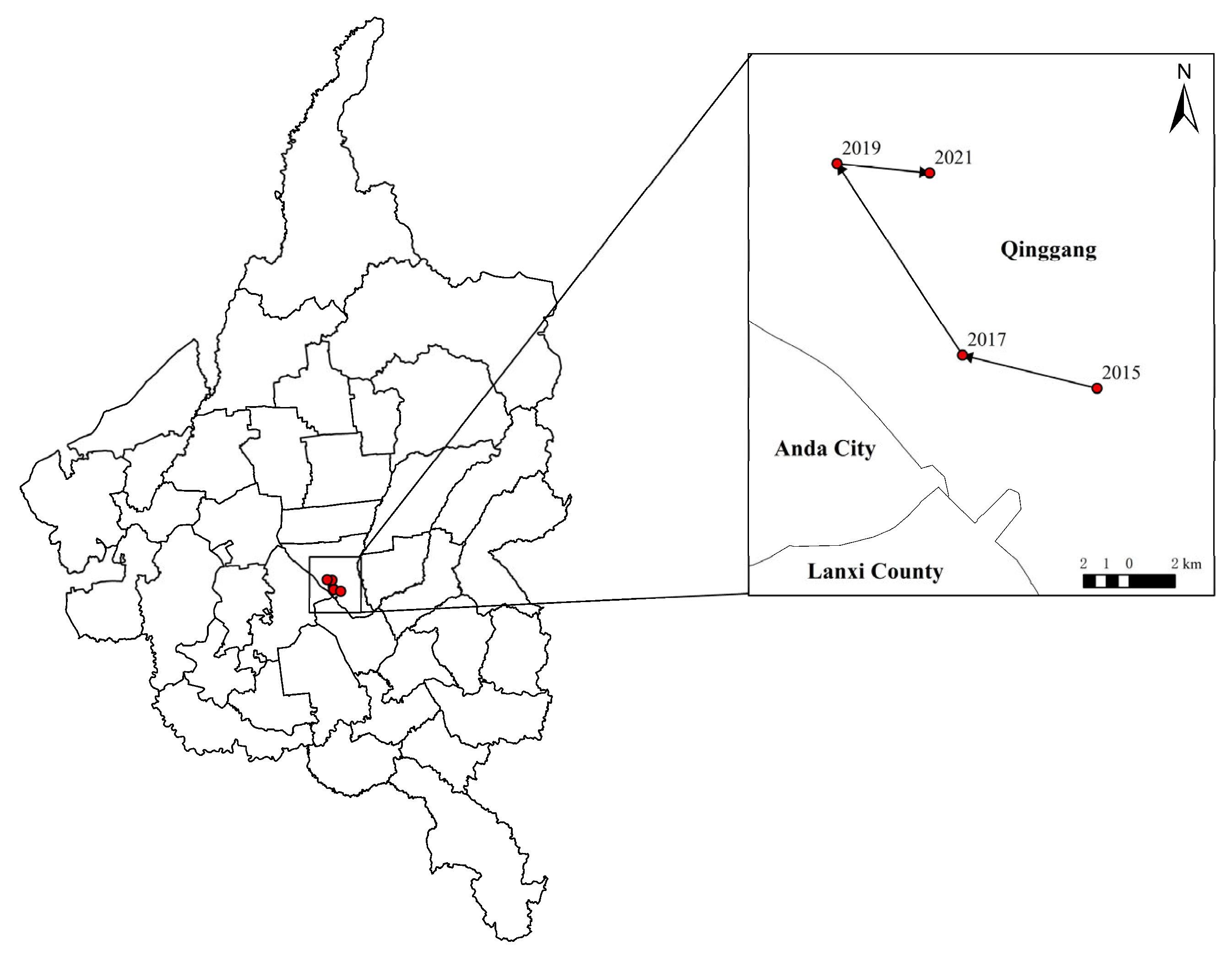
The Standard Deviation Ellipse (SDE) is a spatial analysis method used to describe the central tendency, dispersion, and directional trend of geographic data [73,74]. In this study, SDE was applied to calculate the spatial shift of the grain yield center in the Songnen Plain for the years 2015, 2017, 2019, and 2021. The results are visualized in Figure 14. While the overall shift in the grain yield center across the Songnen Plain is relatively small, a slight northward movement can be observed. This spatial trend is consistent with the patterns identified through Ordinary Kriging, Co-Kriging, and Geographically Weighted Regression (GWR), indicating the reliability and interpretability of the SDE-based findings.

While this study primarily focuses on physical environmental variables due to the availability and consistency of spatial data, it is important to acknowledge that socio-economic and land management factors—such as cultivation practices, irrigation infrastructure, input intensity, and agricultural policy—also play a crucial role in determining grain yield. Empirical evidence has shown that improvements in field management technologies, particularly mechanized cultivation and targeted irrigation, can substantially enhance crop productivity. However, incorporating such human-related variables at a comparable spatial resolution remains challenging due to limitations in data availability and consistency. Future research should aim to integrate these dimensions to develop a more comprehensive understanding of yield variability and to support more holistic and adaptive land management strategies [75,76].

5. Conclusions

(1)

Among the tested configurations, Ordinary Kriging using an exponential kernel and semivariogram with a step length of 13 produced the most accurate interpolation results (RMSE = 0.856), with minimal mean error and balanced standardized error metrics. In contrast, Co-Kriging, which integrated several factors, showed slightly inferior performance (RMSE = 0.891). The results from Geographically Weighted Regression (GWR) were also largely consistent with those of the optimal Ordinary Kriging model.

(2)

The spatial distribution patterns of grain yield described below were obtained using the optimal Ordinary Kriging method. From 2015 to 2017, grain yield increased mainly in the southwestern region, while declines were concentrated in the central zone. Between 2017 and 2019, yield continued to rise in the north and west, with recovery in central areas and new declines in the southeast. From 2019 to 2021, western areas experienced a decrease, whereas yield rose in the eastern and southern parts. Overall, from 2015 to 2021, most of the Songnen Plain showed positive growth in grain yield, especially in the southwest and far north, with only localized reductions in the northern zone.

(3)

Based on per-unit-area calculations, grain yield exhibited significant regional variations in growth rate. The highest increase reached 259.71% (Wudalianchi City), while the greatest decline was 12.20% (Shuangcheng District). These values represent relative changes in productivity, not absolute output. To some extent, this conclusion is consistent with the interpolation results.

(4)

Standard Deviation Ellipse (SDE) analysis indicated a slight northward shift in the grain yield center from 2015 to 2021. This directional trend aligned well with results from Kriging and Geographically Weighted Regression, suggesting consistent spatial dynamics across methods.

(5)

Policy and Practical Recommendations:

Based on the observed spatial and temporal patterns of grain yield, we recommend that policymakers prioritize targeted support and resource allocation to areas experiencing yield instability or decline. Additionally, agricultural practitioners could benefit from adopting location-specific management practices informed by spatial analysis tools such as Kriging and GWR, which can guide precision farming, soil management, and input optimization. These approaches may help enhance productivity while supporting long-term sustainability goals. Overall, this study provides valuable insights into the spatial-temporal dynamics of grain yield in the Songnen Plain, highlighting regional variability and shifts in production centers over time. The integration of advanced spatial analysis methods offers a robust framework for monitoring agricultural productivity. These findings can support more informed land management and policy decisions aimed at enhancing sustainable grain production and regional food security. Spatial yield modeling has proven effective in guiding precision agriculture and supporting regional agricultural planning, especially through the identification of yield gaps and resource optimization [77,78,79]. Future efforts should also strive to integrate socio-economic and management-related variables to complement the physical-environmental framework and improve the explanatory power of spatial yield models.

References

1. Zhang, Y.; Li, B. Detection of the Spatio-Temporal Differentiation Patterns and Influencing Factors of Wheat Production in Huang-Huai-Hai Region. Foods 2022, 11, 1617. [Google Scholar] [CrossRef]
2. Gao, Y.; Yue, Y.; Yang, W. Correlating Grain Yield with Irrigation in a Spatio-Temporal Context on the North China Plain. Heliyon 2024, 10, e32745. [Google Scholar] [CrossRef]
3. Wang, Z.; Zhang, E.; Chen, G. Spatiotemporal Variation and Influencing Factors of Grain Yield in Major Grain-Producing Counties: A Comparative Study of Two Provinces from China. Land 2023, 12, 1810. [Google Scholar] [CrossRef]
4. Leng, G.; Huang, M. Crop Yield Response to Climate Change Varies with Crop Spatial Distribution Pattern. Sci. Rep. 2017, 7, 1463. [Google Scholar] [CrossRef]
5. Ghosh, B.N.; Sharma, N.K.; Alam, N.M.; Singh, R.J.; Juyal, G.P. Elevation, Slope Aspect and Integrated Nutrient Management Effects on Crop Productivity and Soil Quality in North-West Himalayas, India. J. Mt. Sci. 2014, 11, 1208–1217. [Google Scholar] [CrossRef]
6. Chen, D.; Wei, W.; Chen, L.; Ma, B.; Li, H. Response of Soil Nutrients to Terracing and Environmental Factors in the Loess Plateau of China. Geogr. Sustain. 2024, 5, 230–240. [Google Scholar] [CrossRef]
7. Dorji, T.; Odeh, I.; Field, D. Vertical Distribution of Soil Organic Carbon Density in Relation to Land Use/Cover, Altitude and Slope Aspect in the Eastern Himalayas. Land 2014, 3, 1232–1250. [Google Scholar] [CrossRef]
8. Bangroo, S.A.; Najar, G.R.; Rasool, A. Effect of Altitude and Aspect on Soil Organic Carbon and Nitrogen Stocks in the Himalayan Mawer Forest Range. CATENA 2017, 158, 63–68. [Google Scholar] [CrossRef]
9. Li, C.; Shi, W.; Huang, M. Effects of Crop Rotation and Topography on Soil Erosion and Nutrient Loss under Natural Rainfall Conditions on the Chinese Loess Plateau. Land 2023, 12, 265. [Google Scholar] [CrossRef]
10. Zhou, Z.; Jin, J.; Wang, L. Modeling the Effects of Elevation and Precipitation on Rice (Oryza sativa L.) Production Considering Multiple Planting Methods and Cultivars in Central China. Sci. Total Environ. 2022, 813, 152679. [Google Scholar] [CrossRef] [PubMed]
11. Yang, J.; El-Kassaby, Y.A.; Guan, W. The Effect of Slope Aspect on Vegetation Attributes in a Mountainous Dry Valley, Southwest China. Sci. Rep. 2020, 10, 16465. [Google Scholar] [CrossRef]
12. Zhang, Q.; Fang, R.; Deng, C.; Zhao, H.; Shen, M.-H.; Wang, Q. Slope Aspect Effects on Plant Community Characteristics and Soil Properties of Alpine Meadows on Eastern Qinghai-Tibetan Plateau. Ecol. Indic. 2022, 143, 109400. [Google Scholar] [CrossRef]
13. Masoud, M.; Abdul-Hamid, H.; Bin Mohamed, J.; Alsanousi, A. Investigating Soil Properties on the North and South Slopes at Different Elevations in Al-Jabal Al-Akhdar, Libya. For. Sci. Technol. 2024, 20, 286–299. [Google Scholar] [CrossRef]
14. Haile, G.; Gebru, C.; Lemenih, M.; Agegnehu, G. Soil Property and Crop Yield Responses to Variation in Land Use and Topographic Position: Case Study from Southern Highland of Ethiopia. Heliyon 2024, 10, e25098. [Google Scholar] [CrossRef]
15. Johnson, R. Soil-Water Retention and Its Role in Crop Yield Optimization. Int. J. Adv. Chem. Res. 2023, 5, 117–120. [Google Scholar] [CrossRef]
16. Amsili, J.P.; Van Es, H.M.; Schindelbeck, R.R. Cropping System and Soil Texture Shape Soil Health Outcomes and Scoring Functions. Soil Secur. 2021, 4, 100012. [Google Scholar] [CrossRef]
17. Liu, D.; Wang, Z.; Song, K.; Zhang, B.; Hu, L.; Huang, N.; Zhang, S.; Luo, L.; Zhang, C.; Jiang, G. Land Use/Cover Changes and Environmental Consequences in Songnen Plain, Northeast China. Chin. Geogr. Sci. 2009, 19, 299–305. [Google Scholar] [CrossRef]
18. Lu, Z.; Zhang, J.; Li, C.; Dong, Z.; Lei, G.; Yu, Z. Effects of Land Use Change on Runoff Depth in the Songnen Plain, China. Sci. Rep. 2024, 14, 24464. [Google Scholar] [CrossRef] [PubMed]
19. Wang, H.; Wan, Z.; Yu, S.; Luo, X.; Sun, G. Catastrophic Eco-Environmental Change in the Songnen Plain, Northeastern China since 1900s. Chin. Geogr. Sci. 2004, 14, 179–185. [Google Scholar] [CrossRef]
20. Chen, Z.; Zhang, S.; Geng, W.; Ding, Y.; Jiang, X. Use of Geographically Weighted Regression (GWR) to Reveal Spatially Varying Relationships between Cd Accumulation and Soil Properties at Field Scale. Land 2022, 11, 635. [Google Scholar] [CrossRef]
21. Zhang, Y.; Zang, S.; Sun, L.; Yan, B.; Yang, T.; Yan, W.; Meadows, M.E.; Wang, C.; Qi, J. Characterizing the Changing Environment of Cropland in the Songnen Plain, Northeast China, from 1990 to 2015. J. Geogr. Sci. 2019, 29, 658–674. [Google Scholar] [CrossRef]
22. Zhang, L.; Wang, C.; Li, X.; Zhang, H.; Li, W.; Jiang, L. Impacts of Agricultural Expansion (1910s–2010s) on the Water Cycle in the Songneng Plain, Northeast China. Remote Sens. 2018, 10, 1108. [Google Scholar] [CrossRef]
23. Zhang, Y.; Hao, R.; Qin, Y. Temporal and Spatial Variation of Agricultural and Pastoral Production in the Eastern Section of the Agro-Pastoral Transitional Zone in Northern China. Agriculture 2024, 14, 829. [Google Scholar] [CrossRef]
24. Hao, Y.; Wang, Y.; Chang, Q.; Wei, X. Effects of Long-Term Fertilization on Soil Organic Carbon and Nitrogen in a Highland Agroecosystem. Pedosphere 2017, 27, 725–736. [Google Scholar] [CrossRef]
25. Wang, K.; Zhao, X.; Zheng, H.; Zheng, B.; Xu, Y.; Zhang, F.; Duan, Z. The Agro-Pastoral Transitional Zone in Northern China: Continuously Intensifying Land Use Competition Leading to Imbalanced Spatial Matching of Ecological Elements. Land 2024, 13, 654. [Google Scholar] [CrossRef]
26. Hang, Y.; Lu, X.; Li, X. Spatiotemporal Differentiation Characteristics and Zoning of Cultivated Land System Resilience in the Songnen Plain. Sustainability 2025, 17, 4314. [Google Scholar] [CrossRef]
27. Li, H.; Huang, F.; Hong, X.; Wang, P. Evaluating Satellite-Observed Ecosystem Function Changes and the Interaction with Drought in Songnen Plain, Northeast China. Remote Sens. 2022, 14, 5887. [Google Scholar] [CrossRef]
28. Yang, P.; Ames, D.P.; Fonseca, A.; Anderson, D.; Shrestha, R.; Glenn, N.F.; Cao, Y. What Is the Effect of LiDAR-Derived DEM Resolution on Large-Scale Watershed Model Results? Environ. Model. Softw. 2014, 58, 48–57. [Google Scholar] [CrossRef]
29. Osborne, J. Improving Your Data Transformations: Applying the Box-Cox Transformation. Pract. Assess. Res. Eval. 2010, 15, 12. [Google Scholar] [CrossRef]
30. Du, G.; Guo, T.; Ma, C. Effects of Topographic Factors on Cultivated-Land Ridge Orientation in the Black Soil Region of Songnen Plain. Land 2022, 11, 1489. [Google Scholar] [CrossRef]
31. Wu, Y.; Wang, W.; Wang, Q.; Zhong, Z.; Wang, H.; Yang, Y. Farmland Shelterbelt Changes in Soil Properties: Soil Depth-Location Dependency and General Pattern in Songnen Plain, Northeastern China. Forests 2023, 14, 584. [Google Scholar] [CrossRef]
32. Zhao, H.; Luo, C.; Kong, D.; Yu, Y.; Zang, D.; Wang, F. Spatial and Temporal Variations in Soil Organic Matter and Their Influencing Factors in the Songnen and Sanjiang Plains of China (1984–2021). Land 2024, 13, 1447. [Google Scholar] [CrossRef]
33. FAO. A Framework for Land Evalution; FAO Soils Bulletin; 2nd Printing; Soil Resources, Management and Conservation Service, Ed.; FAO: Rome, Italy, 1981; ISBN 978-92-5-100111-0. [Google Scholar]
34. Zhu, Z.; Xie, Y. Research on Evaluation Methods of Black Soil Farmland Productivity Based on Field Block Scale. Appl. Sci. 2024, 14, 3130. [Google Scholar] [CrossRef]
35. Freedman, D.; Diaconis, P. On the Histogram as a Density Estimator: L2 Theory. Z. Wahrscheinlichkeitstheorie Verwandte Geb. 1981, 57, 453–476. [Google Scholar] [CrossRef]
36. Lugosi, G.; Nobel, A. Consistency of Data-Driven Histogram Methods for Density Estimation and Classification. Ann. Statist. 1996, 24, 687–706. [Google Scholar] [CrossRef]
37. Wilk, M.B.; Gnanadesikan, R. Probability Plotting Methods for the Analysis for the Analysis of Data. Biometrika 1968, 55, 1–17. [Google Scholar] [CrossRef] [PubMed]
38. Filliben, J.J. The Probability Plot Correlation Coefficient Test for Normality. Technometrics 1975, 17, 111–117. [Google Scholar] [CrossRef]
39. Almeida, A.; Loy, A.; Hofmann, H. Ggplot2 Compatible Quantile-Quantile Plots in R. R J. 2019, 10, 248. [Google Scholar] [CrossRef]
40. Anselin, L. Local Indicators of Spatial Association—LISA. Geogr. Anal. 1995, 27, 93–115. [Google Scholar] [CrossRef]
41. Getis, A.; Ord, J.K. The Analysis of Spatial Association by Use of Distance Statistics. Geogr. Anal. 1992, 24, 189–206. [Google Scholar] [CrossRef]
42. Maniteja, M.; Samanta, G.; Gebretsadik, A.; Tsae, N.B.; Rai, S.S.; Fissha, Y.; Okada, N.; Kawamura, Y. Advancing Iron Ore Grade Estimation: A Comparative Study of Machine Learning and Ordinary Kriging. Minerals 2025, 15, 131. [Google Scholar] [CrossRef]
43. Wackernagel, H. Ordinary Kriging. In Multivariate Geostatistics; Springer: Berlin/Heidelberg, Germany, 1998; pp. 83–92. ISBN 978-3-662-03552-8. [Google Scholar]
44. Han, H.; Suh, J. Spatial Prediction of Soil Contaminants Using a Hybrid Random Forest–Ordinary Kriging Model. Appl. Sci. 2024, 14, 1666. [Google Scholar] [CrossRef]
45. Dowd, P.A.; Pardo-Igúzquiza, E. The Many Forms of Co-Kriging: A Diversity of Multivariate Spatial Estimators. Math. Geosci. 2024, 56, 387–413. [Google Scholar] [CrossRef]
46. Qu, M.; Guang, X.; Liu, H.; Zhao, Y.; Huang, B. Incorporating Auxiliary Data of Different Spatial Scales for Spatial Prediction of Soil Nitrogen Using Robust Residual Cokriging (RRCoK). Agronomy 2021, 11, 2516. [Google Scholar] [CrossRef]
47. Wang, Y.; Wang, H.; Wang, C.; Zhang, S.; Wang, R.; Wang, S.; Duan, J. Co-Kriging-Guided Interpolation for Mapping Forest Aboveground Biomass by Integrating Global Ecosystem Dynamics Investigation and Sentinel-2 Data. Remote Sens. 2024, 16, 2913. [Google Scholar] [CrossRef]
48. Robertson, F.; Crawford, D.; Partington, D.; Oliver, I.; Rees, D.; Aumann, C.; Armstrong, R.; Perris, R.; Davey, M.; Moodie, M.; et al. Soil Organic Carbon in Cropping and Pasture Systems of Victoria, Australia. Soil Res. 2016, 54, 64. [Google Scholar] [CrossRef]
49. Risk, C.; James, P.M.A. Optimal Cross-Validation Strategies for Selection of Spatial Interpolation Models for the Canadian Forest Fire Weather Index System. Earth Space Sci. 2022, 9, e2021EA002019. [Google Scholar] [CrossRef]
50. Mahoney, M.J.; Johnson, L.K.; Silge, J.; Frick, H.; Kuhn, M.; Beier, C.M. Assessing the Performance of Spatial Cross-Validation Approaches for Models of Spatially Structured Data. arXiv 2023, arXiv:2303.07334. [Google Scholar]
51. Milà, C.; Mateu, J.; Pebesma, E.; Meyer, H. Nearest Neighbour Distance Matching Leave-One-Out Cross-Validation for Map Validation. Methods Ecol. Evol. 2022, 13, 1304–1316. [Google Scholar] [CrossRef]
52. Stock, A.; Subramaniam, A. Iterative Spatial Leave-One-out Cross-Validation and Gap-Filling Based Data Augmentation for Supervised Learning Applications in Marine Remote Sensing. GISci. Remote Sens. 2022, 59, 1281–1300. [Google Scholar] [CrossRef]
53. Düzgün, H.; Kemeç, S. Spatial and Geographically Weighted Regression. In Encyclopedia of GIS; Springer: Boston, MA, USA, 2008; pp. 1073–1077. ISBN 978-0-387-30858-6. [Google Scholar]
54. Yu, S.; Hu, X.; Sheng, Y.; Zhao, C. Similarity and Geographically Weighted Regression Considering Spatial Scales of Features Space. Spat. Stat. 2025, 67, 100897. [Google Scholar] [CrossRef]
55. Quiñones, S.; Goyal, A.; Ahmed, Z.U. Geographically Weighted Machine Learning Model for Untangling Spatial Heterogeneity of Type 2 Diabetes Mellitus (T2D) Prevalence in the USA. Sci. Rep. 2021, 11, 6955. [Google Scholar] [CrossRef]
56. Hong, Z.; Wang, J.; Wang, H. Introducing Bootstrap Test Technique to Identify Spatial Heterogeneity in Geographically and Temporally Weighted Regression Models. Spat. Stat. 2022, 51, 100683. [Google Scholar] [CrossRef]
57. Magno, M.; Luffman, I.; Nandi, A. Evaluating Spatial Regression-Informed Cokriging of Metals in Soils near Abandoned Mines in Bumpus Cove, Tennessee, USA. Geosciences 2021, 11, 434. [Google Scholar] [CrossRef]
58. Usowicz, B.; Lipiec, J.; Łukowski, M.; Słomiński, J. Improvement of Spatial Interpolation of Precipitation Distribution Using Cokriging Incorporating Rain-Gauge and Satellite (SMOS) Soil Moisture Data. Remote Sens. 2021, 13, 1039. [Google Scholar] [CrossRef]
59. Oshan, T.; Li, Z.; Kang, W.; Wolf, L.; Fotheringham, A. Mgwr: A Python Implementation of Multiscale Geographically Weighted Regression for Investigating Process Spatial Heterogeneity and Scale. ISPRS Int. J. Geo-Inf. 2019, 8, 269. [Google Scholar] [CrossRef]
60. Roger, A.; Libohova, Z.; Rossier, N.; Joost, S.; Maltas, A.; Frossard, E.; Sinaj, S. Spatial Variability of Soil Phosphorus in the Fribourg Canton, Switzerland. Geoderma 2014, 217–218, 26–36. [Google Scholar] [CrossRef]
61. Mutiah, S.; Aldi, M.N.; Saefuddin, A.; Ernawati, F. Comparison of Ordinary Kriging and Cokriging for Spatial Estimation Based on Simulated Data. CAUCHY 2025, 10, 533–544. [Google Scholar] [CrossRef]
62. Zhang, H.; Cai, W. When Doesn’t Cokriging Outperform Kriging? arXiv 2015, arXiv:1507.08403. [Google Scholar]
63. García-Soidán, P.; Cotos-Yáñez, T.R. Use of Correlated Data for Nonparametric Prediction of a Spatial Target Variable. Mathematics 2020, 8, 2077. [Google Scholar] [CrossRef]
64. Tziachris, P.; Metaxa, E.; Papadopoulos, F.; Papadopoulou, M. Spatial Modelling and Prediction Assessment of Soil Iron Using Kriging Interpolation with pH as Auxiliary Information. ISPRS Int. J. Geo-Inf. 2017, 6, 283. [Google Scholar] [CrossRef]
65. Yu, Z.; Zhang, X.; Liu, J.; Lei, G. Long-term Effects of Soil Erosion on Dryland Crop Yields in the Songnen Plain, Northeast China. Soil Use Manag. 2024, 40, e13044. [Google Scholar] [CrossRef]
66. Cui, Y.; Liu, S.; Li, X.; Geng, H.; Xie, Y.; He, Y. Estimating Maize Yield in the Black Soil Region of Northeast China Using Land Surface Data Assimilation: Integrating a Crop Model and Remote Sensing. Front. Plant Sci. 2022, 13, 915109. [Google Scholar] [CrossRef] [PubMed]
67. Mo, J.; Song, Z.; Che, Y.; Li, J.; Liu, T.; Feng, J.; Wang, Z.; Rong, J.; Gu, S. Effects of Aeolian Deposition on Soil Properties and Microbial Carbon Metabolism Function in Farmland of Songnen Plain, China. Sci. Rep. 2024, 14, 14791. [Google Scholar] [CrossRef]
68. Andersson Djurfeldt, A. Gendered Land Rights, Legal Reform and Social Norms in the Context of Land Fragmentation—A Review of the Literature for Kenya, Rwanda and Uganda. Land Use Policy 2020, 90, 104305. [Google Scholar] [CrossRef]
69. Chen, J.; Zhu, R.; Zhang, Q.; Kong, X.; Sun, D. Reduced-Tillage Management Enhances Soil Properties and Crop Yields in a Alfalfa-Corn Rotation: Case Study of the Songnen Plain, China. Sci. Rep. 2019, 9, 17064. [Google Scholar] [CrossRef]
70. Tang, B.; Meng, F.; Dong, F.; Zhang, H.; Meng, B. The Spatiotemporal Evolution of Extreme Climate Indices in the Songnen Plain and Its Impact on Maize Yield. Agronomy 2024, 14, 2128. [Google Scholar] [CrossRef]
71. Yang, Q.; Zhang, P.; Ma, Z.; Liu, D.; Guo, Y. Agricultural Economic Resilience in the Context of International Food Price Fluctuation—An Empirical Analysis on the Main Grain–Producing Areas in Northeast China. Sustainability 2022, 14, 14102. [Google Scholar] [CrossRef]
72. Ye, F.; Qin, S.; Li, H.; Li, Z.; Tong, T. Policy-Driven Food Security: Investigating the Impact of China’s Maize Subsidy Policy Reform on Farmer’ Productivity. Front. Sustain. Food Syst. 2024, 8, 1349765. [Google Scholar] [CrossRef]
73. Wang, B.; Shi, W.; Miao, Z. Confidence Analysis of Standard Deviational Ellipse and Its Extension into Higher Dimensional Euclidean Space. PLoS ONE 2015, 10, e0118537. [Google Scholar] [CrossRef]
74. Moore, T.W.; McGuire, M.P. Using the Standard Deviational Ellipse to Document Changes to the Spatial Dispersion of Seasonal Tornado Activity in the United States. npj Clim. Atmos. Sci. 2019, 2, 21. [Google Scholar] [CrossRef]
75. Li, J.; Zhang, H.; Xu, E. Spatialization of Actual Grain Crop Yield Coupled with Cultivation Systems and Multiple Factors: From Survey Data to Grid. Agronomy 2020, 10, 675. [Google Scholar] [CrossRef]
76. He, H.; Ding, R.; Tian, X. Spatiotemporal Characteristics and Influencing Factors of Grain Yield at the County Level in Shandong Province, China. Sci. Rep. 2022, 12, 12001. [Google Scholar] [CrossRef] [PubMed]
77. Rattalino Edreira, J.I.; Andrade, J.F.; Cassman, K.G.; Van Ittersum, M.K.; Van Loon, M.P.; Grassini, P. Spatial Frameworks for Robust Estimation of Yield Gaps. Nat. Food 2021, 2, 773–779. [Google Scholar] [CrossRef]
78. Barrile, V.; Maesano, C.; Genovese, E. Optimization of Crop Yield in Precision Agriculture Using WSNs, Remote Sensing, and Atmospheric Simulation Models for Real-Time Environmental Monitoring. J. Sens. Actuator Netw. 2025, 14, 14. [Google Scholar] [CrossRef]
79. Gumma, M.K.; Nukala, R.M.; Panjala, P.; Bellam, P.K.; Gajjala, S.; Dubey, S.K.; Sehgal, V.K.; Mohammed, I.; Deevi, K.C. Optimizing Crop Yield Estimation through Geospatial Technology: A Comparative Analysis of a Semi-Physical Model, Crop Simulation, and Machine Learning Algorithms. AgriEngineering 2024, 6, 786–802. [Google Scholar] [CrossRef]
Figure 1. Location and overview map of the Songnen Plain in Heilongjiang Province.
Land 14 01705 g001
Figure 2. The methodology framework.
Land 14 01705 g002
Figure 3. Histogram of grain yield after Box–Cox transformation from 2015 to 2021: (a) 2015; (b) 2017; (c) 2019; (d) 2021.
Land 14 01705 g003
Figure 4. Q–Q plots of grain yield after Box–Cox transformation from 2015 to 2021: (a) 2015; (b) 2017; (c) 2019; (d) 2021.
Land 14 01705 g004
Figure 5. Moran scatter plot and LISA aggregation plot of grain yield for the years 2015, 2017, 2019, and 2021: (a) 2015 Moran scatter plot; (b) 2017 Moran scatter plot; (c) 2019 Moran scatter plot; (d) 2021 Moran scatter plot; (e) 2015 LISA aggregation map; (f) 2017 LISA aggregation map; (g) 2019 LISA aggregation map; (h) 2021 LISA aggregation map; (i) 2015 LISA significance map; (j) 2017 LISA significance map; (k) 2019 LISA significance map; (l) 2021 LISA significance map.
Land 14 01705 g005
Figure 6. Ordinary Kriging interpolation results for the years 2015, 2017, 2019, and 2021: (a) 2015; (b) 2017; (c) 2019; (d) 2021.
Land 14 01705 g006
Figure 7. Co-Kriging interpolation results for the years 2015, 2017, 2019, and 2021: (a) 2015; (b) 2017; (c) 2019; (d) 2021.
Land 14 01705 g007
Figure 8. Performance of Ordinary Kriging (OK) and Co-Kriging (CK) under their respective optimal parameter configurations, showing Root Mean Square Error (RMSE), Mean Error (ME), and Root Mean Squared Standardized Error (RMSSE) values.
Land 14 01705 g008
Figure 9. GWR results for the years 2015, 2017, 2019, and 2021: (a) 2015; (b) 2017; (c) 2019; (d) 2021.
Land 14 01705 g009
Figure 10. Histograms of GWR residuals for the years (a) 2015, (b) 2017, (c) 2019, and (d) 2021.
Land 14 01705 g010
Figure 11. Spatial autocorrelation of GWR residuals: (a) Global Moran’s I results; (b) Local Moran’s I (LISA) cluster map.
Land 14 01705 g011
Figure 12. Spatial distribution of local regression coefficients for static explanatory variables: (a) slope, (b) aspect, (c) elevation, and (d) soil type.
Land 14 01705 g012
Figure 13. Spatial changes in grain yield across the Songnen Plain during different periods: (a) 2015–2017, (b) 2017–2019, (c) 2019–2021, and (d) 2015–2021.
Land 14 01705 g013
Figure 14. Spatial shift of the grain yield center in the Songnen Plain based on standard deviation ellipse analysis.
Land 14 01705 g014