Article

How Can We Achieve Carbon Neutrality During Urban Expansion? An Empirical Study from Qionglai City, China

1
College of Resources, Sichuan Agricultural University, Chengdu 611130, China
2
Key Laboratory of Investigation, Monitoring, Protection and Utilization of Cropland Resources, Ministry of Natural Resources, Chengdu 611130, China
3
Observation and Research Station of Land Ecology and Land Use in Chengdu Plain, Ministry of Natural Resources, Chengdu 610045, China
*
Author to whom correspondence should be addressed.
These authors contributed equally to this work.
Land 2025, 14(8), 1689; https://doi.org/10.3390/land14081689
Submission received: 8 July 2025 / Revised: 6 August 2025 / Accepted: 18 August 2025 / Published: 21 August 2025

Abstract

While technologies like renewable energy and low-carbon transportation are known to mitigate carbon emissions from urban expansion, achieving carbon neutrality during this process remains a critical unresolved challenge. This issue is particularly pressing for developing countries striving to balance urbanization with carbon reduction. Taking Qionglai City as a case study, this study simulated the territorial spatial functional patterns (TSFPs) and carbon emission distribution for 2025 and 2030. Based on the key drivers of carbon emissions from urban expansion identified through the Geographical and Temporal Weighted Regression (GTWR) model, carbon-neutral pathways were designed for two scenarios: urban expansion scenarios under historical evolution patterns (Scenario I) and urban expansion scenarios optimized under carbon neutrality targets (Scenario II). The results indicate that (1) urban space is projected to expand from 6094.73 hm2 in 2020 to 6249.77 hm2 in 2025 and 6385.75 hm2 in 2030; (2) total carbon emissions are forecasted to reach 1.25 × 10⁶ t (metric tons) and 1.40 × 10⁶ t in 2025 and 2030, respectively, exhibiting a spatial pattern of “high in the central-eastern regions, low in the west”; (3) GDP, Net Primary Productivity (NPP), and the number of fuel vehicles are the dominant drivers of carbon emissions from urban expansion; and (4) a four-pronged strategy, optimizing urban green space vegetation types, replacing fuel vehicles with new energy vehicles, controlling carbon emissions per GDP, and purchasing carbon credits, proves effective. Scenario II presents the optimal pathway: carbon neutrality in the expansion zone can be achieved by 2025 using the first three measures (e.g., optimizing 66.73 hm2 of green space, replacing 800 fuel vehicles, and maintaining emissions at 0.21 t/104 CNY per GDP). By 2030, carbon neutrality can be achieved by implementing all four measures (e.g., optimizing 67.57 hm2 of green space, replacing 1470 fuel vehicles, and achieving 0.15 t/104 CNY per GDP). This study provides a methodological basis for local governments to promote low-carbon urban development and offers practical insights for developing nations to reconcile urban expansion with carbon neutrality goals.

1. Introduction

Global warming has intensified in recent years, with extreme weather, rising sea levels, and biodiversity loss threatening sustainable development [1]. As the primary greenhouse gas, carbon dioxide (CO2) accounts for approximately 66% of radiative forcing and directly drives roughly 76% of global warming [2]. Accelerated urbanization, marked by population influx and construction land expansion, has further fueled CO2 emissions [3]. Research indicates that land use change, increased energy consumption, population agglomeration, and shifting economic patterns driven by urbanization are key contributors to rising emissions [3]. Over the past four decades, China has undergone rapid urbanization, with a continuously increasing proportion of its urban population and significant expansion of urban scales leading to substantial changes in land use [4]. Since the launch of the reform and opening-up policy in 1978, China’s urbanization rate has surged from 20% to approximately 64% by 2020. This process has been accompanied by a rapid increase in carbon emissions, making China one of the world’s largest CO2 emitters, accounting for about 27% of the global total [2,5]. Rapid urbanization also leads to ecological land loss, further accelerating emissions [6]. In response, China proposed dual carbon targets: peaking by 2030 and neutrality by 2060 [7]. However, as a developing country, China must avoid both restricting urbanization at the cost of growth and allowing unchecked expansion [8,9]. Therefore, balancing urbanization with carbon emission control and exploring low-carbon pathways during urban expansion is not only crucial for guiding China towards its “dual carbon” strategic goals but can also offer valuable lessons for global urban development and climate governance.
As the core manifestation of the global urbanization process, urban expansion, with its spatiotemporal patterns, driving mechanisms, and environmental effects, has become a research hotspot in geography, ecology, and urban planning [10,11]. Currently, numerous methods or models are available for simulating urban expansion, such as traditional Cellular Automata (CA), Land Use and Cover Change (LUCC) models, and the emerging Patch-generating Land Use Simulation (PLUS) model [12,13,14]. Among these, the PLUS model, by integrating a random forest algorithm to identify drivers of land use change and combining it with a multi-type cellular automaton to simulate the patch generation process, offers significant advantages in capturing the spatial self-organization characteristics of urban expansion and the non-linear relationships among multiple driving factors [14]. For example, Li et al. [15] employed a Genetic Algorithm (GA) and the PLUS model to optimize the quantitative structure and spatial layout of Production–Living–Ecological Land (PLEL) in Ningbo City, respectively. This provided technical support for decision-makers in formulating targeted territorial spatial plans and achieving regional sustainable development. Compared to traditional models, the PLUS model demonstrates superior performance in multi-scenario simulation, dynamic response, and complex system interaction analysis. It is particularly well-suited for synergistic research on urban expansion and carbon neutrality goals, showing broad application prospects.
Current carbon emission accounting methods mainly include direct measurement, material balance, factor decomposition, life cycle assessment, and the emission factor method recommended by the IPCC [16,17,18,19]. Among these, the emission factor method, proposed by the IPCC Greenhouse Gas Inventory Guidelines, has become the most widely applied approach due to its complete methodological framework and standardized parameters, which support analyses at both global and regional scales. However, this method involves a complex calculation process, has high data quality requirements, and possesses limited regional applicability [5,20,21]. In contrast, the land use carbon emission coefficient method is better suited for carbon emission accounting in regions with limited data resources or at smaller study scales, owing to its simpler data requirements and ease of spatial distribution expression [20]. A key limitation, however, is that its fixed coefficients cannot account for the spatiotemporal differences in carbon emissions or ecosystem interactions [22]. Currently, carbon emission accounting is predominantly focused on administrative units, such as provinces, cities, and counties [23,24]. A few studies have extended this work to the level of urban agglomerations [25,26], yet these approaches still struggle to capture the fine-scale spatial heterogeneity of emissions. In contrast, grid-based accounting offers a high-resolution depiction of carbon emission distributions at the sub-city scale [22]. It is noteworthy that existing grid-based spatial simulations of carbon emissions are mostly based on land use/land cover (LULC) classification, with few simulations conducted from the perspective of territorial spatial function (TSF) utilization [27]. Accordingly, by integrating the IPCC inventory method with the carbon emission coefficient approach—and fully accounting for local industrial structure, energy consumption patterns, and data availability—we conducted grid-cell carbon emission spatial distribution simulations. This framework overcomes the limitations of traditional administrative- or regional-scale accounting, which cannot capture fine-scale spatial heterogeneity, and achieves high-precision modeling of carbon emissions in both space and time.
The main drivers of carbon emission changes include the energy mix, industrial structure, territorial development intensity, functional land use structure, economic development level, and population size [28,29,30]. Mainstream methods for analyzing carbon emission drivers include the Logarithmic Mean Divisia Index (LMDI) decomposition method, Environmental Input–Output Structural Decomposition Analysis (EIO-SDA), the Structural Path Decomposition (SPD) method, Gray Relational Analysis, the SPNN-GNNWR model, Geodetector, and Geographically and Temporally Weighted Regression (GTWR) [24,31,32,33,34,35,36]. Although the LMDI method is widely used for decomposing carbon emission drivers due to its operational simplicity, it neglects the spatiotemporal heterogeneity of these drivers, making it difficult to reveal their varying impacts across time and space [37]. In contrast, the GTWR model can capture both spatial and temporal variability and has been widely used in land use carbon emission studies [38,39]. For example, Shi et al. [40] employed the GTWR model to study the spatiotemporal impacts of urban form on CO2 emissions and found significant spatiotemporal heterogeneity in this relationship. It is noteworthy that existing research has primarily focused on analyzing the impacts of carbon emission changes across entire regions, while studies specifically addressing the influencing factors of carbon emissions during the urban expansion process remain relatively scarce. Although significant progress has been made in understanding the interaction mechanisms between urbanization and carbon emissions in recent years, for instance, Wu et al. [41], after analyzing territorial carbon sink conflicts in the Yangtze River Delta urban agglomeration, pointed out that urban expansion leads to the conversion of ecological land and a reduction in carbon storage. Vasenev et al. [42] further noted that the disruption of biogeochemical processes in peri-urban areas leads to a decrease in soil organic carbon content, exacerbating carbon emissions. Due to the significant impact of urbanization on carbon emissions, controlling the scale of urban expansion has become a common practice for achieving carbon neutrality. However, this has a huge impact on the economies of developing countries, which are accelerating their urbanization process, and is not in line with the actual situation in developing countries [43]. While some studies emphasize that low-carbon or even zero-emission urbanization may be achievable through measures such as urban greening, energy-efficient buildings, and green transportation [44,45], existing research has not conducted a systematic quantitative analysis [46,47] and thus has not truly addressed how to achieve zero emissions in the process of urban expansion. Further in-depth investigation is urgently needed.
Despite progress in urban expansion simulation, carbon accounting, and driver identification, three main gaps remain. First, most carbon emission spatial simulations focus on administrative units (provinces, cities, and counties), with few fine-grained grid-based studies combined with TSFs, limiting accurate spatial heterogeneity characterization. Second, research mainly examines emissions and drivers at a broad scale, lacking detailed spatiotemporal analysis of drivers during urban expansion, causing policies to rely on linear extrapolation, which is inadequate for complex carbon-neutral scenarios. Third, while some low-carbon pathways address greening, energy saving, and green transport, a systematic zero-emission strategy specifically for urban expansion is missing. Therefore, achieving net-zero carbon during urban expansion by optimizing TSFs’ layout, regulating drivers, and designing emission reduction strategies remains a critical challenge for developing countries that are in the process of balancing carbon control and growth.
To address these issues, this study first constructs an urban expansion driver index system and uses the PLUS model to simulate the urban spatial distribution of Qionglai City for 2025 and 2030. Second, we develop a TSF-based carbon emission accounting framework by integrating land use emission coefficients with the IPCC method to simulate urban carbon emissions from 2010 to 2020. We then apply the LSTM model to predict the spatial distribution of net emissions for 2025 and 2030. Next, a GTWR model analyzes the spatial heterogeneity of emission drivers during urban expansion to identify key factors. Finally, we establish historical evolution and carbon neutrality-constrained scenarios and formulate zero-carbon pathways for 2025 and 2030 based on these drivers. This study aims to provide empirical evidence and technical pathways for local governments like Qionglai City to promote low-carbon urban development and offer insights for developing countries balancing urban expansion with climate mitigation.

2. Materials and Methods

2.1. Study Area and Data

2.1.1. Overview of the Study Area

Qionglai City, located in western China between the Chengdu Plain and Longmen Mountains (30°12′ N–30°33′ N, 103°04′ E–103°45′ E), covers 1377 km2 and includes 1 street, 19 towns, and 4 townships (Figure 1). The terrain slopes northwest to southeast, ranging from 451 m to 1991 m, and consists of plains (mainly east and northeast), mountains (mainly south and west), and hills (central and northwest). Rivers extend 271 km, providing abundant water resources. The city experiences a subtropical humid monsoon climate, with an average temperature of 16.3 °C, annual precipitation of around 1117 mm, 1108 sunshine hours, and evaporation of 1025 mm. Soils are mainly fluvo-aquic and purple soils, and forest vegetation is dominated by subtropical evergreen broadleaf forests in mountainous and hilly areas.
In this study, we selected Qionglai City as our case study to explore pathways for achieving carbon emissions during urban expansion. This choice was based on two primary considerations. First, since 2010, its trends in urbanization, economy, population, and carbon emission intensity closely resemble those of typical Chinese cities and developing countries like India, Brazil, and South Africa, reflecting shared challenges in land transformation, energy adjustment, and carbon changes amid rapid urbanization. Second, Qionglai emphasizes ecological civilization and climate governance, has set clear carbon neutrality goals, and faces similar governance needs [48]. Therefore, this case not only guides Qionglai’s low-carbon development but also provides policy and theoretical support for comparable regions.
Figure 1. Geographical location of the research area [49].
Land 14 01689 g001

2.1.2. Data Sources and Processing

The data used in this study mainly include raster data, vector data, and panel data (Table 1). To meet the data analysis requirements, all data types were standardized: the geographical coordinate system was set to WGS-1984, the projected coordinate system to UTM, and the raster resolution to 100 m × 100 m. Based on this, the panel data underwent primary preprocessing, which mainly involved spatialization. The panel data comprises two categories: socioeconomic development statistics and energy statistics. Socioeconomic data, aggregated at municipal and township levels, were spatialized onto a 100 m × 100 m vector grid following Ou et al. [49]. Energy-consumption parameters were obtained from [50,51] and the China Energy Statistical Yearbook. Notably, due to the absence of energy consumption and chemical oxygen demand (COD) data in industrial wastewater for Qionglai City, we estimated these values using data from Chengdu city or Sichuan Province. Specific methods include the following: urban production energy consumption is equal to Chengdu’s comprehensive energy consumption per 104 CNY of industrial output (above-scale enterprises) multiplied by the study area’s industrial output value; urban domestic energy consumption is equal to Chengdu’s per capita consumption of electricity, natural gas, and liquefied petroleum gas multiplied by the study area’s urban population; rural domestic energy consumption is equal to Chengdu’s rural per capita consumption of electricity, natural gas, and liquefied petroleum gas multiplied by the study area’s rural population; and chemical oxygen demand in industrial wastewater is equal to Sichuan Province’s average COD concentration multiplied by the ratio of the study area’s industrial output to that of Sichuan Province [52,53,54,55,56].

2.2. Methodology

2.2.1. Urban Spatial Expansion Simulation Using the PLUS Model

Development of a Driver Indicator System for Urban Expansion
Research indicates that the process of urban expansion is jointly influenced by topography and geomorphology, the natural environment, transportation accessibility, and socio-economic factors [57,58]. To clarify the driving mechanisms of these factors on the functional evolution of territorial space, we systematically screened the core factors that significantly influence urban expansion in Qionglai City, following the principles of scientific validity, relevance, and data availability. Based on this, we constructed a driving factor indicator system (Table 2) (Detailed calculation method is provided in Table S1 of Supplementary Materials).
Topographical factors determine the ease of land development and the direction of expansion. Altitude restricts development in highland areas due to its influence on temperature, oxygen levels, and construction costs. Slope impacts both development costs and the risk of natural disasters, making areas with steep gradients difficult to develop. Topographic relief reflects landscape complexity, with areas of poor connectivity being unconducive to spatial agglomeration and urban sprawl. Consequently, altitude, slope, and topographic relief were selected as the representative topographical indicators.
Natural environmental factors support and constrain urban development through ecological services. Water conservation capacity affects water supply and agricultural layout. Evapotranspiration regulates microclimate and water cycles, mitigating urban heat islands. Environmental purification capacity influences carrying capacity and pollution control costs. Soil conservation reflects nutrient levels and erosion prevention, underpinning agricultural sustainability. Habitat quality indicates ecosystem stability and biodiversity, providing buffering and landscape services. Consequently, water resource conservation, evapotranspiration, environmental purification services, soil conservation, and habitat quality were selected to constitute the natural environment indicators.
Transportation location factors serve as exogenous drivers, influencing factor mobility and accessibility. Higher transportation network density enhances inter-regional connectivity, driving the dispersion of population and resources towards urban peripheries. In addition, the accessibility of public service facilities impacts residential convenience and regional attractiveness, thereby accelerating population and industrial agglomeration. Consequently, transportation network density and public service accessibility were selected to constitute the transportation location indicators.
Socio-economic factors provide the endogenous momentum for urban expansion. Population density reflects the intensity of land demand, as high-density areas compel cities to expand outward due to the demand for housing and services. Per capita GDP measures the level and vitality of economic development; economically robust areas typically exhibit higher levels of urbanization and continuously enhanced spatial functions. Consequently, population density and per capita GDP were selected to constitute the socio-economic indicators.
Simulation of Urban Expansion Using the PLUS Model
The PLUS model, an extension of cellular automata, integrates LEAS and CARS modules, effectively explaining driving factors behind land use changes with high simulation accuracy [14]. The LEAS module samples land expansion across categories between two periods and applies a random forest algorithm to identify drivers and calculate expansion probabilities. The CARS module employs a competitive mechanism with a decreasing threshold to control random seeds, generating new land use patches in a natural growth process. This approach mitigates the probability of unlimited patch expansion, thereby permitting new patches to evolve freely within these constraints [59].
In this study, we predicted the territorial spatial functional patterns (TSFP) of Qionglai City for 2025 and 2030, with a focus on urban space evolution. The specific workflow was as follows: Firstly, we constructed a driving factor indicator system and utilized the LEAS module to quantify the contribution of each factor to functional expansion, thereby generating an expansion probability map. Secondly, we employed the CARS module, using the quantity of each functional type in the base year as the spatial demand. We then simulated the spatial distribution in conjunction with the probability map and compared the results with the actual distribution to evaluate accuracy, which involved pre-selecting parameters such as the seed probability of the random patch and the neighborhood effect. Subsequently, we predicted future spatial demand using a Markov chain model. Finally, we used this projected demand as input for the CARS module, invoking the validated expansion probability map and simulation parameters to simulate the functional distribution for 2030, respectively, thereby revealing future urban expansion trends.

2.2.2. Spatial Simulation of Carbon Emissions from TSFs

Currently, Simulation methodologies for the spatial distribution of carbon emissions from TSFs remain scarce. This study employs a spatial-unit–based framework to model carbon emissions from TSFs. The framework construction steps are as follows: First, we compiled a list of carbon emissions from county-level land use functions and referred to both carbon emissions and absorption as carbon emissions, with positive values representing carbon sources and negative values representing carbon sinks. Secondly, we calculate total carbon emissions for each TSF and derive corresponding emission coefficients. Finally, we divide the study area into spatial units, compute net emissions per unit, and produce a TSFP of carbon emissions from TSFs (Figure 2).
Carbon Emission Inventory of TSFs
In this study, we build upon the previously established county-level TSF classification system [49] and integrate the advantages of the land use carbon emission coefficient method with the IPCC inventory approach to develop a carbon emission inventory for TSFs. Qionglai City’s territorial space is divided into six primary TSFs: urban production space (UPS), urban living space (ULS), urban ecological space (UES), rural production space (RPS), rural living space (RLS), and rural ecological space (RES) [49]. Further, based on the IPCC 2006 National Greenhouse Gas Inventory Guidelines (2019 revision) [51], we classify carbon sources into five sectors: terrestrial ecosystems, energy consumption, waste, population and livestock, and others. Finally, by linking different TSFs with land use categories and aligning land use types with carbon emission items, we establish a carbon-emission inventory corresponding to each TSF (Table 3).
Accounting for Total Carbon Emissions and Coefficient Calculation of TSFs
(1) Total carbon emissions accounting
In the previously constructed TSF carbon-emission inventory, an indirect method based on land use carbon emission coefficients (Detailed calculation method is provided in Table S2 of Supplementary Materials) was used to estimate terrestrial ecosystem emissions, with parameters referenced from existing studies. Emissions from energy consumption, waste, and respiration by humans and animals were calculated directly (Detailed calculation method is provided in Table S3 of Supplementary Materials). Regional carbon emissions include direct and some indirect emissions, incorporating only electricity, heat, cooling, and steam imported from outside the city, while excluding embedded emissions from commodities like building materials and food to avoid unclear boundaries and excessive accounting. Furthermore, referencing relevant studies [60,61], only two major greenhouse gases, carbon dioxide and methane, were accounted for, focusing on primary gases and simplifying the process.
(2) Calculation of carbon emission coefficients
The net carbon emission coefficient for each TSF, including urban production, urban living, urban ecological, rural production, rural living, and rural ecological spaces, is calculated by dividing the total carbon emissions of each type by its total area. The formula used is as follows:
ψ k = j = 1 5 C n e t k j A k
where   ψ k denotes the net carbon emission coefficient for the k t h TSF (Detailed calculation results are provided in Table S4 of Supplementary Materials)   C n e t k j represents the carbon emissions of the j t h carbon emission source within the k t h TSF; A k is the area of the k t h TSF; j and k denote the project and category codes for carbon emissions associated with TSFs, respectively, with k = 1,2 , 3 , , N .
Calculation of Carbon Emissions for Territorial Spatial Units
Firstly, the Create Fishnet tool in Esri ArcGIS 10× (Environmental Systems Research Institute (ESRI), Redlands, CA, USA.) was used to generate territorial spatial units based on Qionglai City’s vector boundary. After balancing accuracy and efficiency, a 100 m × 100 m grid was chosen, totaling 1.40 × 10⁵ units, as it captures both macro patterns and local details [62,63]. On this basis, we applied the Tabulate Intersection tool to overlay the fishnet grid with the TSF classification layers for each year. This yielded a table of area values A i k for each of the six functional space types within each grid cell. We then multiplied A i k by the corresponding net carbon emission coefficient ψ k (calculated using Equation (1) in Section Accounting for Total Carbon Emissions and Coefficient Calculation of TSFs) for that year to generate spatial distribution maps of carbon emissions from 2010 to 2020. The carbon emission per unit was calculated as follows:
C t o t a l i = k = 1 N ψ k A i k
where C t o t a l i denotes the carbon emissions of the i t h territorial spatial unit; A i k represents the area of the k t h TSF within the i t h territorial spatial unit; i is the index of the territorial spatial unit, where   i = 1,2 , , 139736 ; ψ k , k carries the same meaning as defined in Equation (1).
Spatial Distribution Forecast of Carbon Emissions by TSFs
The Long Short-Term Memory (LSTM) is a time series-based prediction tool and represents an advanced algorithmic model of the RNN. A key capability of the LSTM is its ability to predict data for a subsequent time period based on an existing data sequence. Its selective memory function enables it to process large sample sizes without encountering the vanishing or exploding gradient problems commonly found in traditional RNNs. LSTM has demonstrated notable efficacy in time series prediction of carbon emissions, yielding substantial application outcomes [64]. Consequently, we opted to employ the LSTM model to predict the time series of carbon emissions within Qionglai City’s territorial space. We used the net carbon emissions of each 100 m × 100 m grid cell for 2010, 2012, 2014, 2016, 2018, and 2020 (derived from the results in Section Calculation of Carbon Emissions for Territorial Spatial Units) as input features. These six time-point values were concatenated into a sequence of length six, which was then fed into the LSTM model for training and prediction, yielding estimates of net carbon emissions for 2025 and 2030. To assess prediction accuracy, three evaluation metrics were selected: mean absolute error (MAE), root mean square error (RMSE), and determination coefficient (R2). The formulas for these metrics are as follows:
M A E = 1 n i = 1 n y ^ i y i
R M S E = 1 n i = 1 n y i y ^ i 2
R 2 = i = 1 n y ^ i y ¯ 2 i = 1 n y i y ¯ 2
where y ^   i denotes the predicted value, y i the observed value, and y ¯ the mean of the observed values. Both MAE and RMSE range from [0, +∞), with lower values indicating reduced error and higher model accuracy. The coefficient of determination R 2 ranges from [0, 1], where higher values correspond to lower error and greater model precision.

2.2.3. Zero-Emission Pathway Design for Urban Expansion Based on Scenario Analysis

Identification of Key Drivers Influencing Carbon Emissions from Urban Expansion
Urban expansion and carbon emissions show marked spatiotemporal heterogeneity, necessitating analytical tools that capture both dimensions. This study adopts the GTWR model to identify key drivers, as it extends Geographically Weighted Regression (GWR) by incorporating time, thus enabling local regression on panel data across space and time. This helps address sample size limitations and spatiotemporal non-stationarity, improving result accuracy. The dependent variable is defined as the net carbon emission change due to urban expansion. The specific calculation steps were as follows: First, expansion areas for each stage were delineated by comparing the observed spatial patterns in 2010, 2015, and 2020 [49] with the simulated expansion patterns for 2025 and 2030 generated by the PLUS model. Then, using the Spatial Join tool in ArcGIS, each expansion area was spatially linked to the corresponding grid-level net carbon emissions for the relevant year (with emission data for 2010, 2015, and 2020 obtained from the calculations in Section Calculation of Carbon Emissions for Territorial Spatial Units, and data for 2025 and 2030 derived from the LSTM model predictions in Section Spatial Distribution Forecast of Carbon Emissions by TSFs). Finally, the net carbon emission changes within expansion areas for the four periods—2010–2015, 2015–2020, 2020–2025, and 2025–2030—were aggregated into separate panel datasets to serve as the dependent variables in the GTWR model.
Based on previous studies [65] and considering the availability of data and the suitability of quantitative methods for the variables used, six explanatory variables were selected to identify key drivers of carbon emissions during urban expansion (Table 4). The mathematical formulation of the GTWR model is expressed as follows:
y i = β 0 μ i , ν i , t i + k β k μ i , ν i , t i X i k + ε i
where y i   denotes the carbon emissions from urban expansion in the i t h spatial unit;   β 0   represents the intercept;   μ i , ν i and t i correspond to the latitude, longitude, and temporal coordinate of the centroid of the i t h spatial unit, respectively;   β k   signifies the estimated coefficient of the k t h influencing factor for the i t h spatial unit;   X i k     is the value of the k t h influencing factor in the i t h spatial unit; a n d   ε i denotes the stochastic error term.
Scenario-Based Design of Carbon-Neutral Pathways for Urban Expansion
We designed two pathways for achieving carbon neutrality in the expansion of urban space in Qionglai City in 2025 and 2030. Based on this, we designed specific strategies for implementing the scenarios and, through comparative analysis, determined the optimal path for achieving carbon neutrality during urban expansion.
(1) Scenario I: Urban expansion scenarios under historical evolution patterns
This scenario assumes that by 2025 and 2030, the scale and spatial layout of urban production, living, and ecological spaces in Qionglai City will follow historical land use and emission trends. Such “historical continuation” scenarios are widely applied in studies on urban expansion and carbon emissions [66,67], serving as a baseline reference in the absence of policy interventions. They help assess the effectiveness and feasibility of various emission reduction strategies. Based on a carbon source–sink balance, compensation strategies are proposed to offset residual emissions, prioritized as: optimizing urban green space vegetation types, replacing fuel vehicles with new energy vehicles, controlling carbon emissions per GDP, and purchasing carbon credits.
(2) Scenario II: Urban expansion scenarios optimized under carbon neutrality targets
In this scenario, the TSFP no longer follows historical development trends but is instead simulated based on the strategic goal of “carbon neutrality,” aiming to optimize spatial development in a way that coordinates urban expansion and carbon emission reduction. Specifically, the scenario first takes into account the dual objectives of minimizing net carbon emissions and maximizing economic benefits for the years 2025 and 2030. Using constraints such as urban construction land expansion, farmland protection, ecological security, and population size, a multi-objective constrained optimization model is constructed to determine the spatial scale of each TSF. The model expression is as follows:
m i n Z 1 = i = 1 6 a i x i , t m a x Z 2 = i = 1 6 b i x i , t s . t .   i = 1 6 x i , t = A t x 1 , t + x 2 , t + x 3 , t A u , t x 6 , t A e , t x 4 , t A f x 5 , t P t × S x i , t 0 , i = 1,2 , , 6
where Z 1 represents the net carbon emission objective function value, denoting the annual total carbon emissions of various TSFs in Qionglai City under a given spatial layout; Z 2 denotes the economic growth objective function value, reflecting the annual total economic benefits under the same layout. a i ( i = 1 , , 6 ) correspond to the net carbon emission factors for each TSF; b i ( i = 1 , , 6 ) represent the economic benefit coefficients for each TSF; x i , t ( i = 1 , , 6 ) ; t { 2025,2030 } indicate the spatial area of the   i t h TSF in year t, where x 1 , t , x 2 , t , x 3 , t , x 4 , t , x 5 , t , x 6 , t correspond to urban production, urban living, urban ecological, rural production, rural living, and rural ecological spaces, respectively; A t denotes the total area of Qionglai City’s territorial space; A u , t is the scale of urban construction land in planning year t; A e , t represents the ecological redline protection area in year t; A f is the baseline area for farmland protection; P t is the total rural registered population in Qionglai City in 2025; S is the per capita homestead area standard for Chengdu City.
Then, based on the optimized quantitative structure and the TSF suitability evaluation results, the PLUS model is applied to simulate the specific distribution patterns of urban space. Although the spatiotemporal distribution of net carbon emissions under this scenario continues the historical evolution trend, the optimization of TSFs to balance economic benefits and carbon reduction reduces emission intensity to some extent. Finally, to address the remaining carbon deficits following TSF layout optimization, the same compensation-strategy priorities as in Scenario 1 are implemented to design specific zero-emission measures.

3. Results and Analysis

3.1. Simulation Results and Analysis of Urban Space Expansion

3.1.1. Characteristics of the Quantitative Structure of Urban Expansion

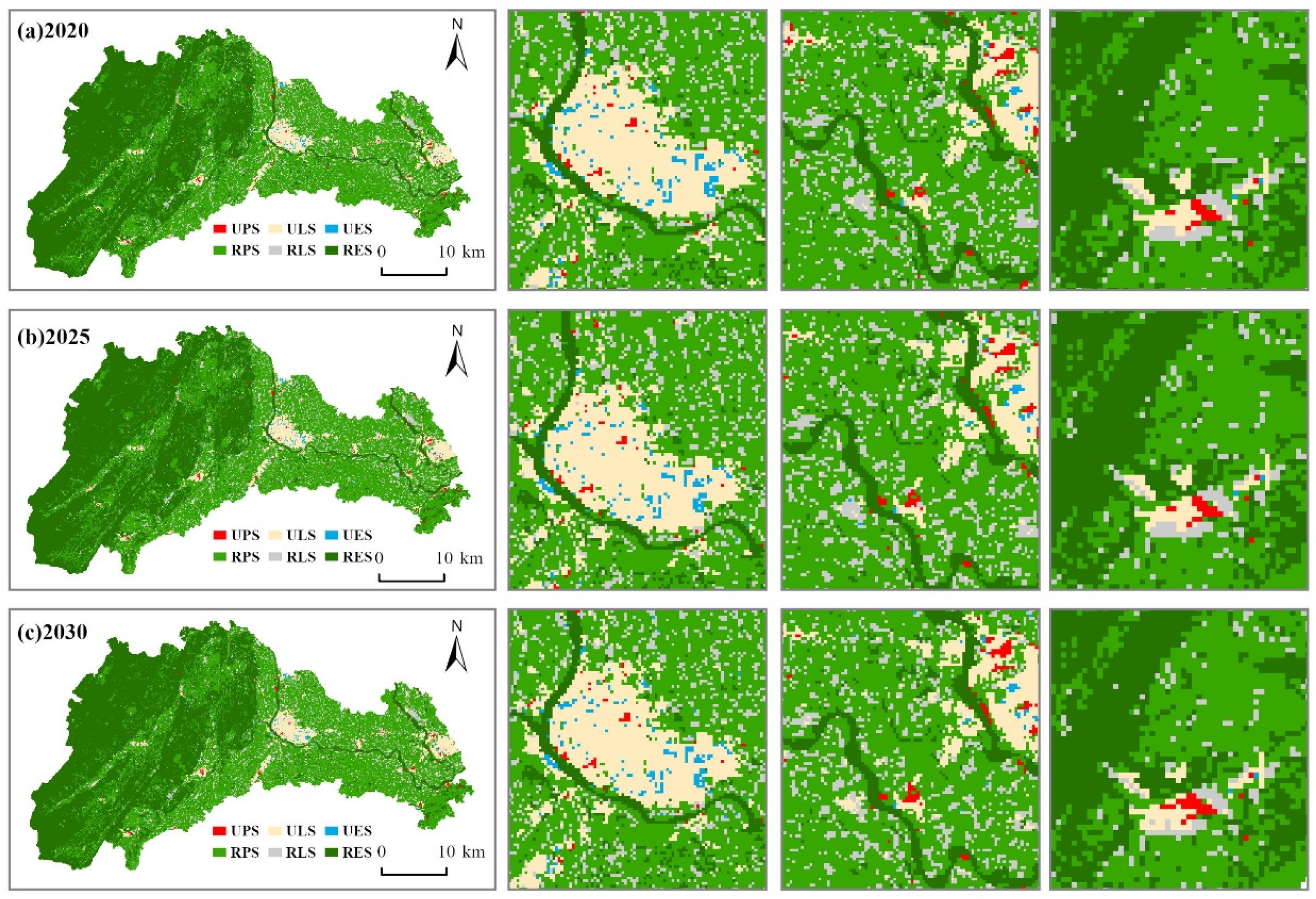
In 2025, the urban space in Qionglai City is projected to reach an area of 6249.77 hm2, accounting for 4.54% of the city’s total territorial space. This represents an increase of 154.10 hm2 compared to the base year (2020). Within this urban space, ULS constitutes the largest component at 5258.95 hm2 (3.90% of the city’s total territorial space), followed by UPS at 521.61 hm2 (0.38%), while UES is the smallest, at only 363.18 hm2 (0.26%).
By 2030, the area of urban space in Qionglai City is projected to continue to climb, reaching 6385.75 hm2. This will account for 4.64% of the city’s total territorial space, representing an increase of 291.02 hm2 compared to the base year (2020). Within this urban space, ULS will remain the largest component, at 5474.75 hm2 (3.98% of the city’s total territorial space); UPS will follow, at 536.81 hm2 (0.39%); and UES will be the smallest, at 374.19 hm2 (0.27%).
In contrast, the area of rural space is projected to decrease from 131,628.44 hm2 in 2020 to 131,473.39 hm2 in 2025, and to further reduce to 131,337.41 hm2 by 2030. Consequently, its proportion of Qionglai City’s total territorial space is expected to decline from 95.57% in 2020 to 95.46% in 2025, and then to 95.36% in 2030 (Table 5).
Compared with the base year, the scale of urban space in the target years (2025 and 2030) is projected to grow steadily, though not significantly. This limited increase is attributed, on one hand, to the “Construction Planning Outline for the Chengdu-Chongqing Dual-City Economic Circle,” which secures land for industrial upgrading through the secondary development of existing construction land. On the other hand, it stems from the slowdown in Qionglai City’s population growth and the new urbanization strategy’s shift from large-scale expansion to quality improvement, with a greater emphasis on tapping the potential of existing land, thereby inhibiting overall growth. In terms of functional distribution, ULS is dominant, primarily influenced by the concentration of rural populations in urban areas and the urban-rural land quota linkage mechanism. UPS is developing intensively to meet the policy requirement for the “efficient utilization of production space.” Driven by the “Park City” concept and the integrated park system of mountains, rivers, forests, farmlands, lakes, and grasslands, UES is steadily improving. However, its growth remains limited due to multiple constraints, including arable land protection policies, mountainous terrain, and the demand for land for urban renewal. Meanwhile, rural space continues to shrink, a trend consistent with the strategy of enhancing the intensive use of rural land.

3.1.2. Spatial Distribution Characteristics of Urban Expansion

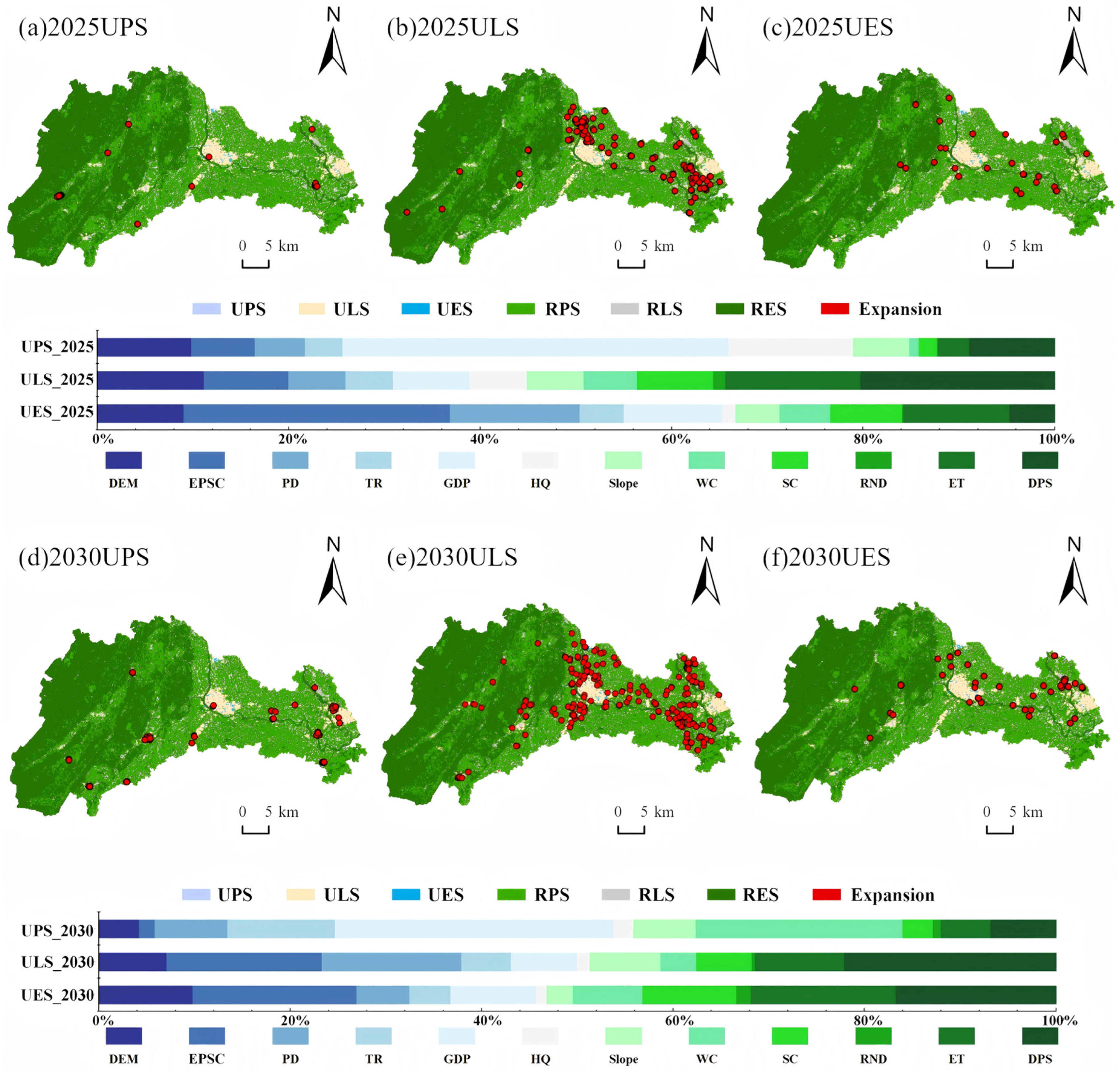
The planned target years (2025 and 2030) for urban spatial distribution are primarily concentrated in the central and eastern regions (Figure 3 and Figure 4).
UPS is primarily concentrated in towns such as Linqiong, Yang’an, Pingle, and Sangyuan. These towns possess strong industrial foundations, well-developed transportation networks, and abundant land resources, which collectively support the intensive layout and large-scale development of production land. ULS is predominantly clustered in towns including Linqiong, Yang’an, and Wolong. These areas are characterized by dense populations, comprehensive public service facilities, and favorable living environments, enabling them to meet the multi-level living needs of residents and accommodate the ongoing urbanization process. UES is more sparsely distributed across towns like Wenjun, Linqiong, Yang’an, and Sangyuan. Such areas are often situated along river corridors or at the peripheries of forested land, holding significant ecological value. They fulfill ecological functions as green spaces and wetlands, forming a dispersed yet interconnected system of ecological corridors that underpins the city’s sustainable development.
The expansion of new UPS occurred sporadically, spreading outwards from the core production areas of the base year. This pattern was driven by GDP, as significant regional economic agglomeration effects attracted investment and promoted industrial spillover. In contrast, the new ULS exhibited an annular expansion pattern, radiating outwards. This was primarily prompted by the accessibility of public service facilities, which spurred population migration and the extension of residential demand. The expansion of UES was limited, with growth mainly originating from the ecological transformation of RLSs. This is because the restoration of green spaces and wetlands improved environmental quality and enhanced ecological service capabilities, thereby fostering the gradual growth of ecological space.

3.2. Simulation Results and Analysis of Carbon Emission Distribution in Territorial Space

3.2.1. Temporal Characteristics of Carbon Emissions from TSFs

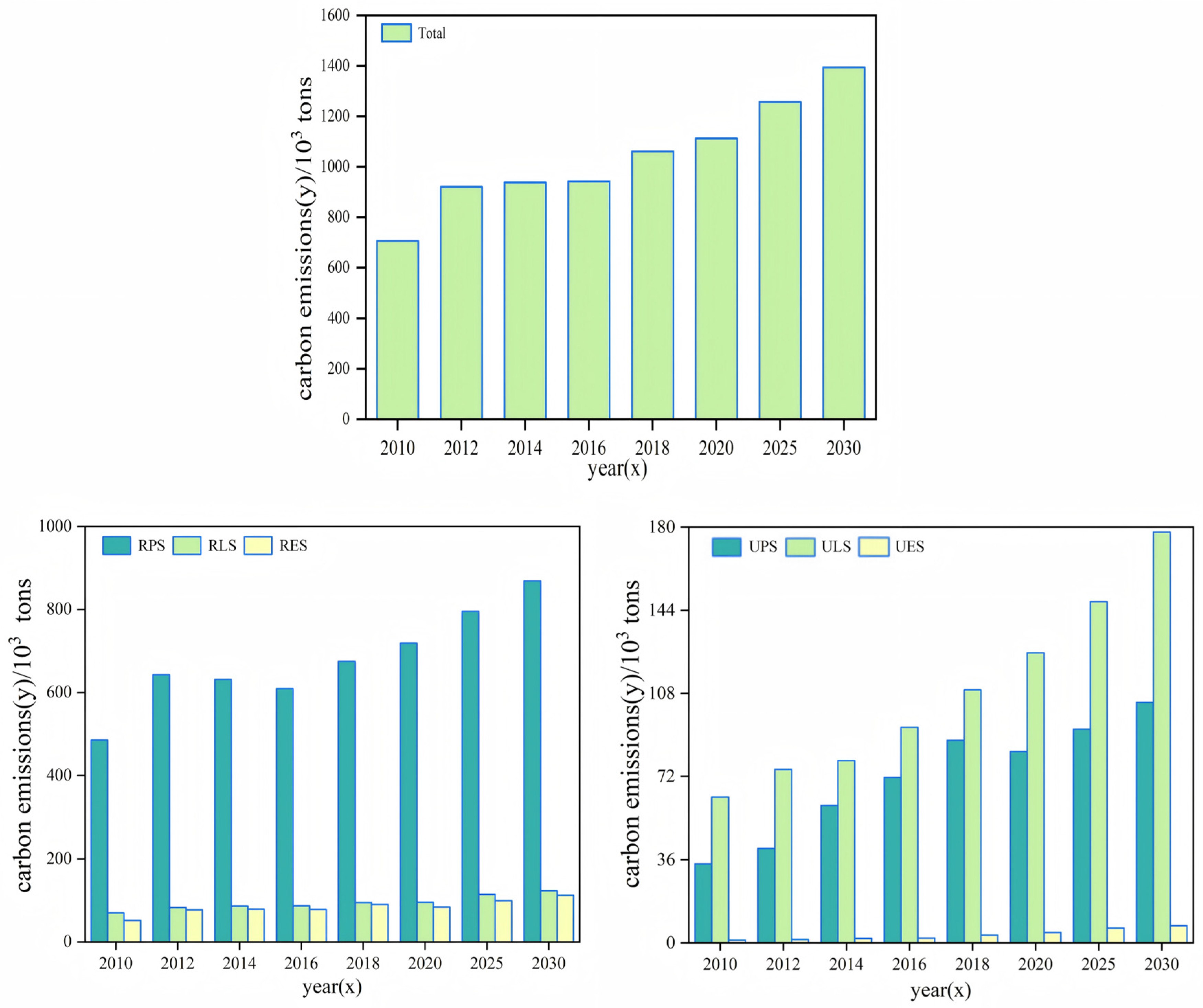
Over the period 2010–2030, the carbon emissions from Qionglai City’s territorial space are observed and projected to follow a pattern characterized by three historical growth phases and two future phases of slower increase: rapid growth (2010–2012), a stabilization period (2012–2016), a moderate rebound (2016–2020), and slow growth (2025–2030) (Figure 5). The city’s total carbon emissions rose from 706,367.34 t in 2010 to 1.11 × 10⁶ t in 2020. During this period, emissions from urban production, living, and ecological spaces increased by 47,067.35 t, 58,035.10 t, and 5768.85 t, respectively. Concurrently, emissions from rural production, living, and ecological spaces increased by 235,031.97 t, 29,735.40 t, and 28,557.74 t, respectively. This reflects the rapid industrialization and urbanization of Qionglai City over the past decade, as well as the significant increase in energy demand and the continuous improvement of transportation infrastructure. Notably, the carbon emissions from ecological spaces are positive. This is attributed to the mixed-patch pattern of land use; even though ecological land possesses carbon sink capabilities, these are insufficient to offset the emissions from the large number of interspersed, high-emission, non-ecological plots.
Between 2010 and 2020, the average annual growth rate of carbon emissions was 4.61%. The fastest growth occurred during 2010–2012, with an average annual rate of 14.12%, primarily driven by the construction of the Tianfu New Area Qionglai Industrial Park, which spurred a surge in industrial energy consumption. From 2012 to 2016, the growth rate slowed to its lowest point of 0.59%. This was due to Qionglai’s designation as a key ecological functional zone, which increased ecological land, and the inclusion of local enterprises in a carbon emissions trading scheme, which reduced emissions by approximately 53,000 t annually. Subsequently, from 2016 to 2020, the growth rate rebounded to 4.26%, following the opening of the Chengdu-Ya’an Railway and the development of rural tourism. Projections indicate that net emissions will reach approximately 1.26 × 106 t by 2025 and rise to 1.40 × 106 t by 2030. This suggests that without accelerated structural adjustments and policy interventions, it is unlikely that Qionglai City will naturally achieve its carbon peak during the 14th and 15th Five-Year Plan periods.

3.2.2. Spatial Characteristics of Carbon Emissions from TSFs

Analysis of Historical Spatial Variations
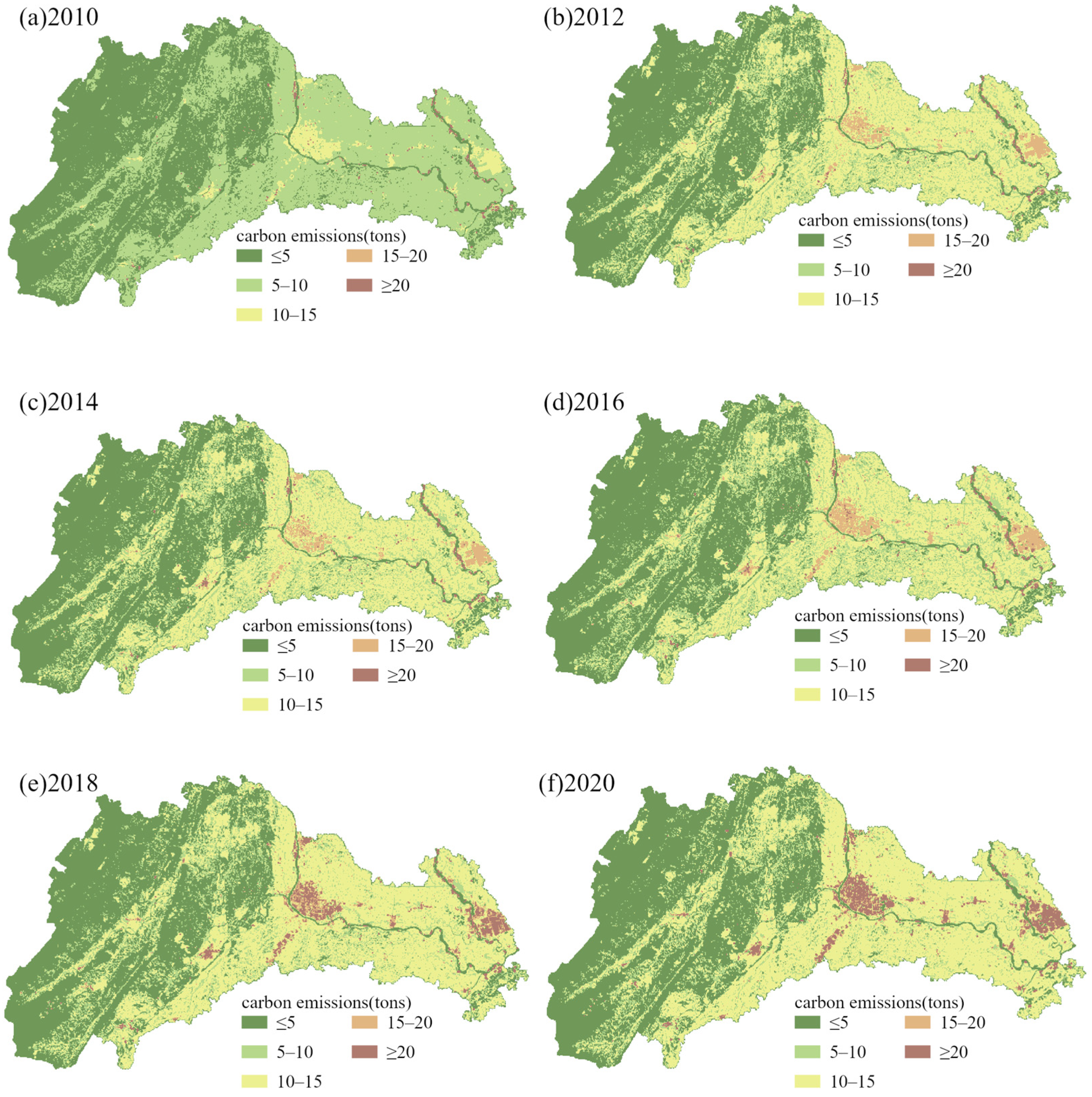
The carbon emissions from various TSFs in Qionglai City between 2010 and 2020 were classified into five types: Low (≤5 t), Relatively Low (>5–10 t), Moderate (>10–15 t), Relatively High (>15–20 t), and High (>20 t) emission (Figure 6). Accelerated urbanization and industrial agglomeration spurred the conversion of agricultural and ecological land into production and living areas. This led to the continuous expansion of population- and industry-dense zones and the progressive improvement of infrastructure and transportation networks, which in turn drove the sustained outward spread and intensification of high-emission areas. Specifically, in 2010, Qionglai City was predominantly characterized by Relatively Low emissions, while the central and eastern regions exhibited Moderate emissions. A few high-emission areas were concentrated in UPSs along the banks of the Nanhe and Xiejiang Rivers. By 2014, the emission levels of some ULSs in the central and eastern parts had escalated from Moderate to Relatively High. Between 2014 and 2016, the Relatively High emission zones gradually expanded outwards, with some central areas further transitioning to High emission status. Subsequently, from 2016 to 2020, the net carbon emission levels of urban areas in the central and eastern parts rose from Relatively High to High. Additionally, driven by infrastructure improvements and rising living standards, rural living and production spaces gradually expanded from Moderate to Relatively High emission zones. In contrast, rural ecological space largely maintained its Low emission pattern.
Analysis of Future Spatial Evolution Trends
Relying solely on the carbon sink function within ecological spaces is insufficient for achieving carbon neutrality. Effective emission control necessitates optimizing the territorial spatial structure, strengthening land management, and implementing targeted emission reduction policies to realize sustainable development goals. Specifically, projections for 2025 indicate that high-emission zones in the central and eastern urban areas of Qionglai City will further expand from their 2020 extent, with a continued intensification of carbon emissions in both urban living and production spaces. Concurrently, agricultural modernization is expected to increase energy consumption, causing some RPSs to escalate from Moderate to Relatively High emission levels. By 2030, ongoing urbanization and agricultural modernization will continue to drive growth in energy consumption and net emissions. Urban living and production spaces are projected to be almost entirely encompassed by high-emission zones, while large areas of RPS are also expected to transition to the high-emission category. Furthermore, within ecological spaces, the carbon sequestration capabilities of water bodies, forests, and grasslands cannot fully offset the emissions from other intermingled land uses. Consequently, the carbon emissions from rural ecological spaces are projected to rise from Low to Relatively Low levels. Meanwhile, UESs are expected to shift from Low to Moderate emission levels, influenced by pressures from adjacent industries, frequent traffic, and population concentration (Figure 7).

3.3. Identification and Analysis of Factors Influencing Carbon Emissions from Urban Expansion

3.3.1. Selection of Influencing Factors

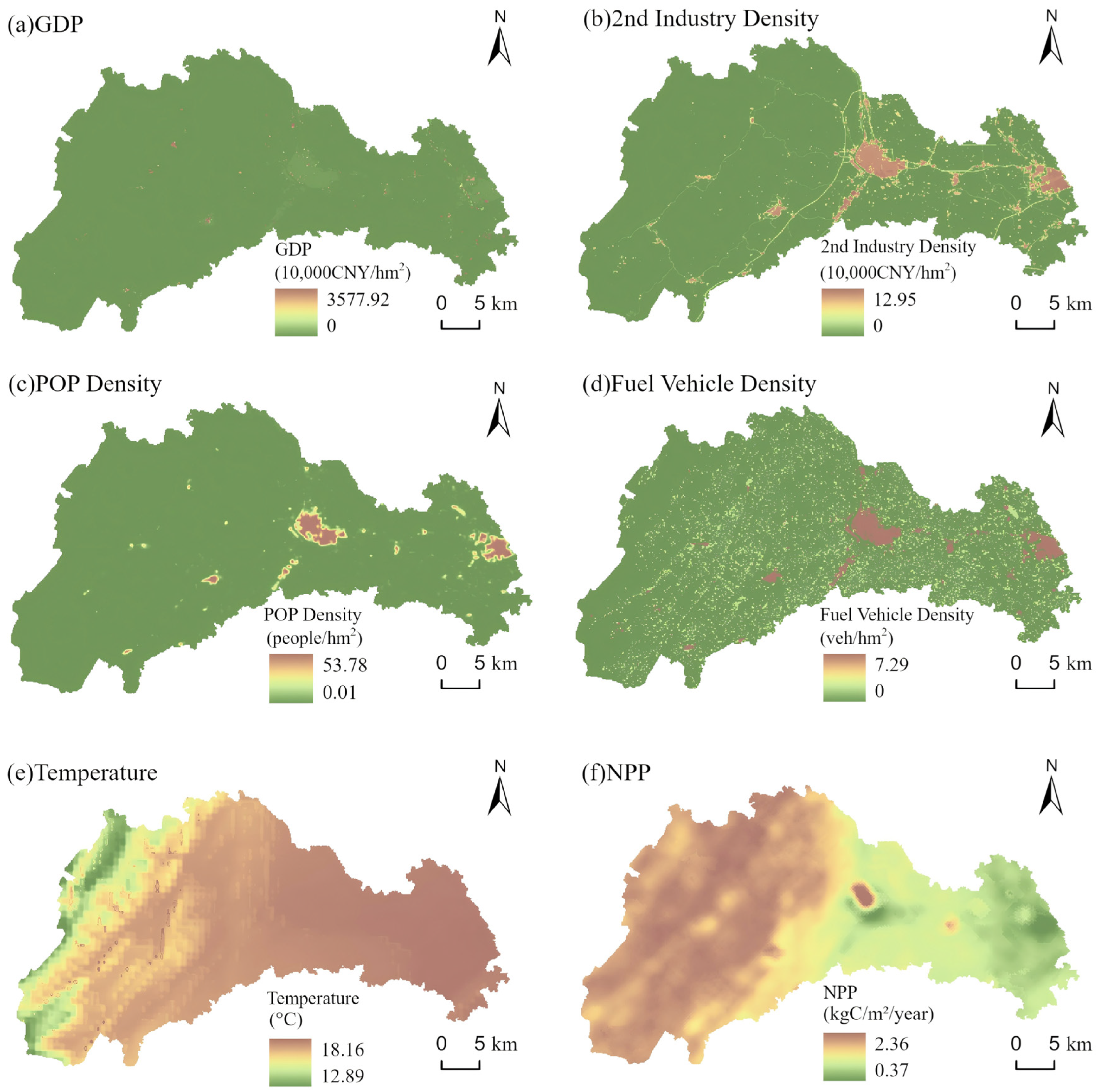
To select the factors influencing carbon emissions from urban expansion, this study first employed Pearson correlation analysis and subsequently conducted a variance inflation factor (VIF) test to ensure the model’s scientific validity and robustness. Through this screening process, six key explanatory variables were ultimately identified: GDP per unit area, secondary industry output density, population density, the number of fuel vehicles, annual average temperature, and NPP (Figure 8).

3.3.2. Exploring the Driving Factors of Carbon Emissions During Urban Expansion Using the GTWR Model

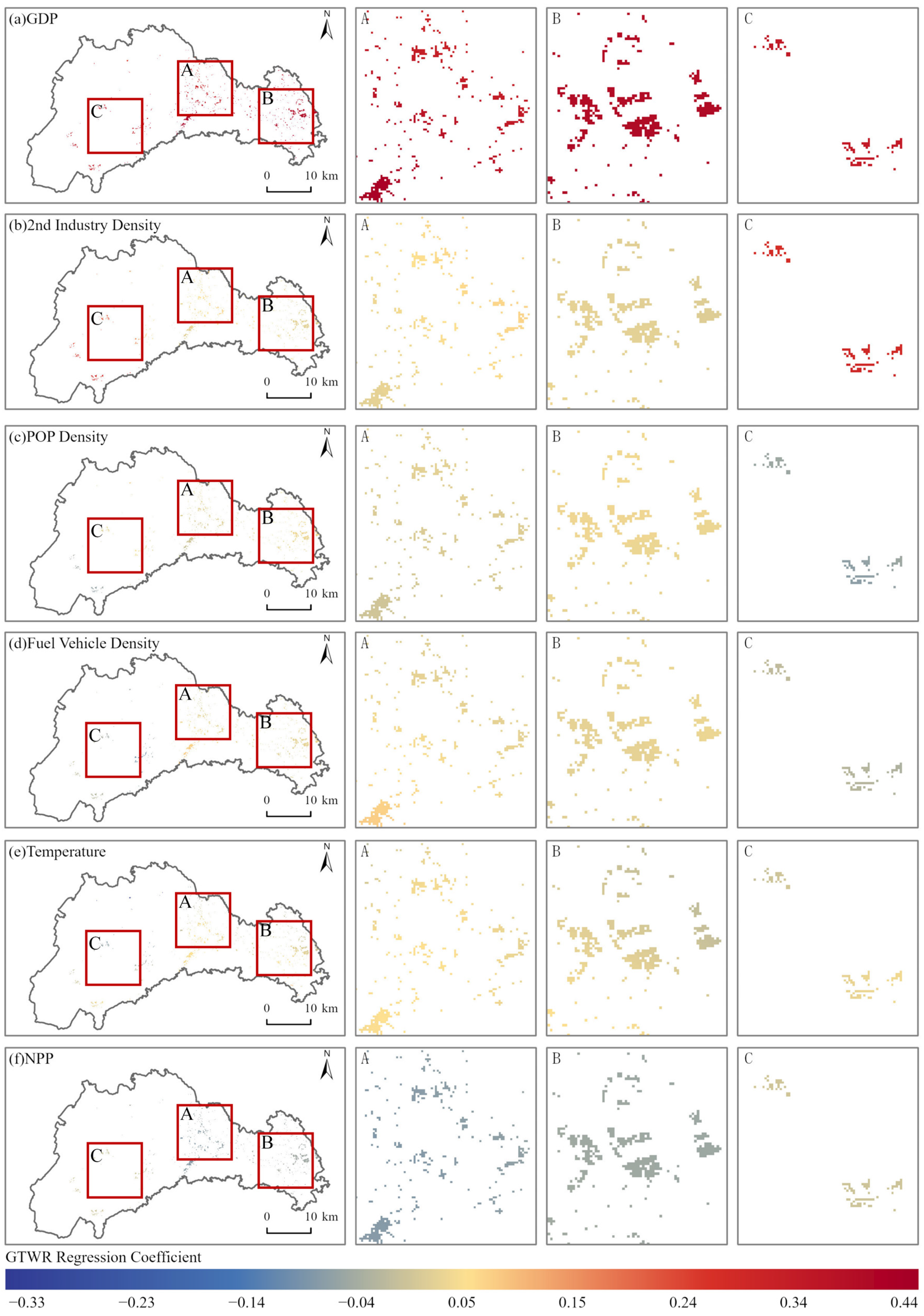
A GTWR analysis was conducted on the six selected factors influencing carbon emission changes associated with urban expansion. The analysis yielded a coefficient of determination (R2) of 0.61, indicating a good model fit (Figure 9). Furthermore, the GTWR parameters for each factor were statistically summarized, encompassing the maximum, minimum, median, and mean values of the regression coefficients, as well as the proportions of positive and negative coefficients (Table 6).
The primary drivers of carbon emissions from urban expansion are GDP per unit area, secondary industry output density, motor vehicle ownership, population density, and annual average temperature. These factors exert a significant positive promoting effect, with GDP per unit area and secondary industry output density notably exhibiting a 100% positive coefficient proportion. In contrast, NPP has a negative coefficient and acts to inhibit emissions. In terms of spatial distribution, the high values of GDP per unit area regression coefficients are concentrated in the central urban area and the eastern plains. This is because this region is home to functional zones such as food processing industrial parks and modern seed industry parks, where high-intensity industrial activities not only boost regional GDP but also significantly increase carbon emissions. The high values of secondary industry output density are distributed in the southwestern mountainous areas, as this region relies on resource-based industries such as alcohol production bases, mineral processing, and heavy chemical projects, whose production activities have a significantly high carbon emission intensity. High values for the number of fuel vehicles and population density are concentrated in the central urban area and eastern regions. This is because, on the one hand, the increase in the number of motor vehicles directly leads to rising carbon emissions from the transportation sector, and on the other hand, high population density areas exhibit significant building energy consumption and residential carbon emissions; The spatial effects of annual average temperature on carbon emissions vary: cities in the central and eastern regions exhibit a positive effect due to higher temperatures leading to increased cooling energy consumption, while mountainous areas in the west exhibit a negative effect due to lower temperatures suppressing energy consumption; The negative inhibitory effect of NPP is primarily evident in the central agricultural regions, followed by the eastern regions, where high biological productivity effectively enhances carbon sink capacity.

3.4. Analysis of Zero-Emission Pathways for Urban Expansion

3.4.1. Analysis of Carbon Emission Control Pathways for Urban Expansion Scenarios Under Historical Evolution Patterns

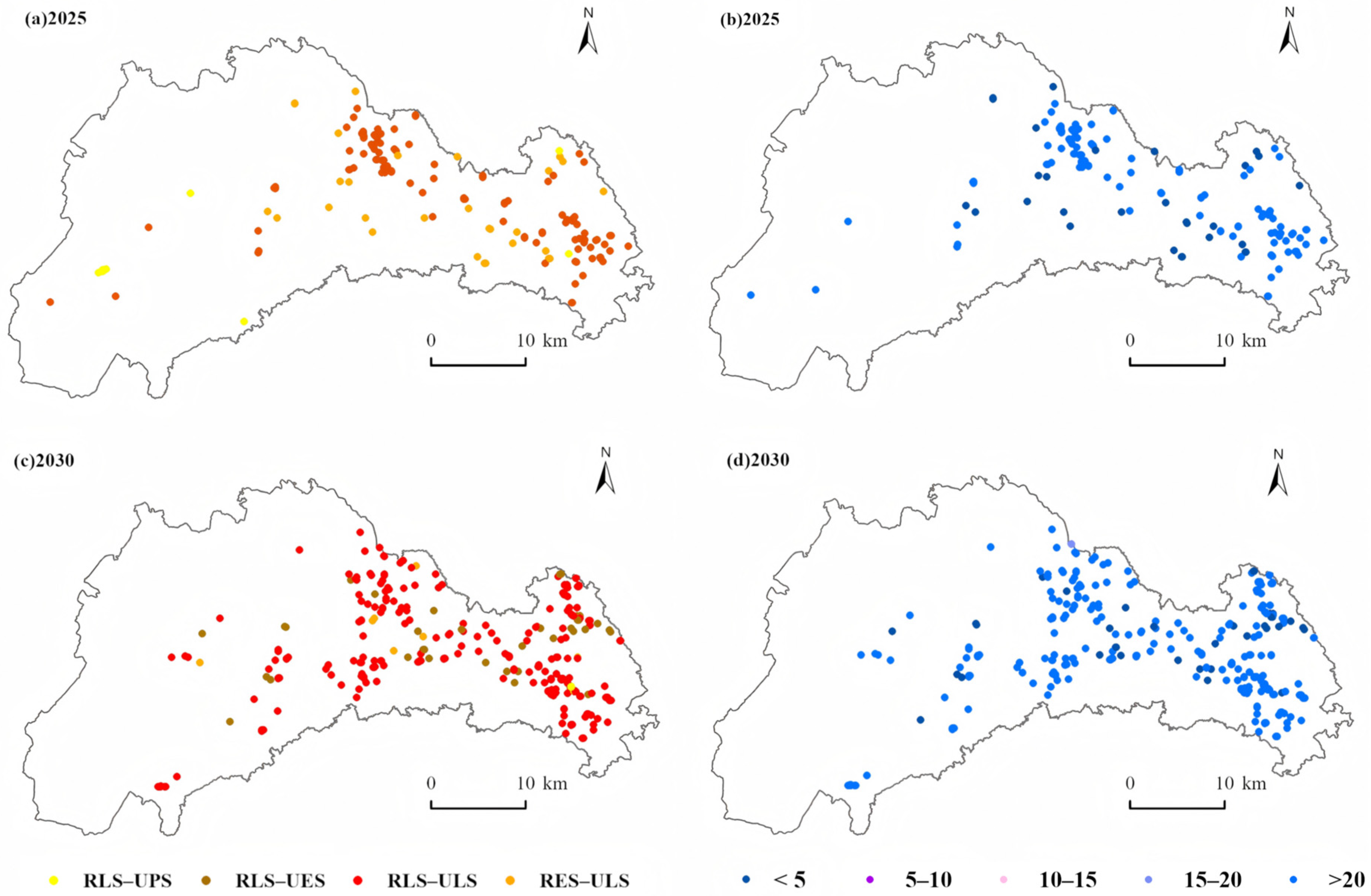
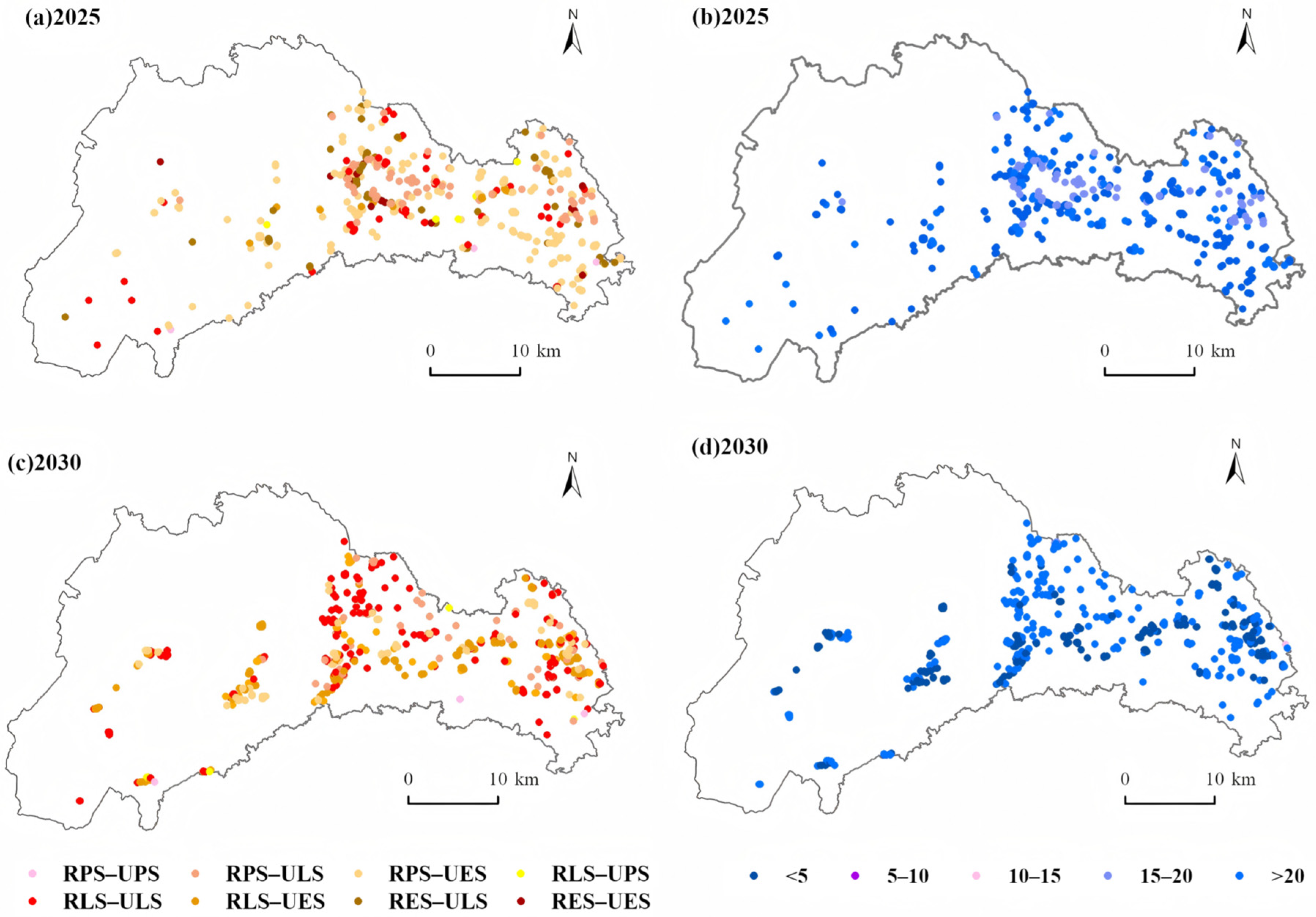
Under the historical evolution model, new carbon emissions resulting from the expansion of production and living space are projected to far exceed the carbon sink increments generated by ecological succession, making it difficult for these sinks to offset emissions. From 2020 to 2030, the conversion patterns among TSFs are expected to be relatively consistent: a small portion of RLS will be converted into urban production or ecological space, a large portion will be transformed into ULS, and some rural ecological space will also be converted into ULS. By 2025, the net emissions from newly added spatial units are projected to be approximately 6035.50 t. Of this total, new production and living land will emit 3909.00 t and 2387.30 t, respectively, while new ecological land will provide a carbon sink of 260.80 t. Areas with high emission intensity are concentrated in the residential fringe zones undergoing transformation from rural living areas, whereas ecologically transformed zones will serve as the primary carbon sinks. By 2030, net emissions are anticipated to rise to 7206.90 t. This includes a significant increase in emissions from living land (to 6463.30 t) and an enhanced ecological carbon sink of 340.00 t. The overall emission pattern is expected to remain largely similar to that of 2025. Concurrently, economic activity will be significantly enhanced. The GDP from these newly expanded areas is projected to increase from 7.35 × 10⁸ CNY in 2025 to 9.58 × 10⁸ CNY in 2030 (Figure 10).

3.4.2. Analysis of Carbon Emission Control Pathways for Urban Expansion Scenarios Under Carbon Neutrality Targets

In this study, we optimized the quantitative structure of TSFs by strictly controlling the scale of urban construction land, adhering to ecological protection red lines, and maintaining the retained amounts of arable land and homestead land. This optimization path prioritizes the enhancement of ecological carbon sinks while simultaneously ensuring the steady growth of production land and the balanced development of living land (Table 7). Following this optimization, we projected that by 2025, UPS would increase by approximately 1.34% compared to the baseline, while ULS would remain largely consistent with the baseline scenario. In contrast, UES is anticipated to expand by about 21.51%. By 2030, we forecast that production space will grow by approximately 3.87%, living space will remain largely unchanged, and ecological space will expand by about 28.44%. Subsequently, we employed the PLUS model to spatially reallocate land uses according to this optimization plan. (The spatial distribution map is shown in Figure S1 of the Supplementary Materials) The results show that new production space tends to scatter around the periphery of the base-year production areas. New living space radiates outward from existing clusters. Significantly, the newly added ecological space originates not only from the ecological transformation of rural living land but also includes the conversion of rural production land to ecological land, a strategy that markedly enhances the regional carbon sink capacity.
In terms of carbon emission control, projections for 2025 indicate that the net emissions from new urban space will be approximately 3782.70 t, a 37.33% decrease from the baseline scenario. This total comprises a carbon sink of 3261.00 t from new ecological land, alongside emissions of 2687.70 t from new production land and 4356.00 t from new living land. Over 56% of the grid cells are expected to achieve zero or negative emissions. High-emission zones are concentrated in the marginal areas where former rural production and living land have been converted to production land. Conversely, areas with significant carbon sink advantages are located in the transition zones converted to ecological land, which are connected to existing ecological corridors and possess favorable ecological conditions. By 2030, RLS is anticipated to be substantially reduced and restructured into urban living and ecological spaces. The net emissions from new urban space are projected to be approximately 7206.90 t, a 4.47% decrease from the baseline. This is composed of a 3173.30 t carbon sink from new ecological land, and emissions of 2867.80 t and 7189.90 t from new production and living land, respectively. The spatial patterns of high-emission and carbon sink zones are expected to remain largely consistent with those of 2025 (Figure 11).
Overall, scenario II demonstrates significant synergistic effects in adjusting spatial structure, controlling carbon emissions, and promoting urban growth. In the expansion zone, GDP increased by 135.47% and 133.22% (for 2025 and 2030, respectively) compared to the baseline scenario, achieving a dual leap in both carbon emission reduction and urban growth. This outcome verifies the comprehensive benefits of the model in multi-objective territorial space management.

3.4.3. Designing Zero-Emission Paths for Urban Expansion Under Different Scenarios

In this study, we conducted a quantitative comparison of four strategies—optimizing urban green space vegetation types (by introducing high-carbon-sequestering species like camphor trees), replacing fuel vehicles with new energy vehicles, controlling carbon emissions per GDP, and purchasing carbon credits—under two scenarios. We found that scenario II significantly enhances ecological carbon sink capacity and emission reduction capabilities in the production and transportation sectors by optimizing the spatial layout. This reduces reliance on high-cost, high-difficulty interventions such as industrial structure adjustment and purchasing carbon credits, thereby offering greater advantages in economic viability and technical feasibility for achieving a zero-emission pathway. In scenario 1 for 2025, optimizing urban green space vegetation increased the carbon sink of new UES by 349.84 t; replacing fuel vehicles with new energy vehicles reduced emissions by 24.37 t; and controlling carbon emissions per GDP to 0.20 t/104 CNY cut emissions by 1010.58 t. The remaining 4650.71 t had to be offset by purchasing carbon credits at a cost of 3.23 × 10⁵ CNY. For 2030 under Scenario 1, the ecological carbon sink rose by 422.22 t; vehicle replacement reduced emissions by 44.78 t; and reducing emission intensity to 0.15 t/104 CNY yielded a further 396.70 t reduction, leaving 6343.20 t to be offset through credits costing 4.41 × 10⁵ CNY. In Scenario 2 for 2025, the new ecological space carbon sink surged to 3170.28 t; vehicle replacement cut emissions by 24.37 t; and a modest reduction in carbon intensity to 0.21 t/104 CNY, achieving a 588.05 t cut, was sufficient to reach net-zero without any credit purchases. By 2030, under Scenario 2, the ecological carbon sink climbed to 3210.09 t; replacing fuel vehicles reduced emissions by 44.78 t; and lowering emission intensity to 0.15 t/104 CNY achieved a 1049.89 t reduction, leaving just 2527.64 t to be offset at a cost of 1.79 × 10⁵ CNY.

4. Discussion

4.1. Integrated Analysis of Urban Expansion Impacts on Carbon Emissions and Carbon Sequestration

Numerous studies have shown that urban expansion significantly increases regional carbon emissions due to the growth of construction land, changes in industrial structure, and population agglomeration effects [25,68,69]. Urban construction expansion not only directly drives the consumption of large amounts of fossil fuels but also alters land use and land cover types, exacerbating the reduction in terrestrial ecological carbon pools and thereby leading to an increase in carbon emissions [70]. In particular, the extensive encroachment on ecological land, such as forests and grasslands, during urban expansion leads to a significant decline in regional ecological carbon sink capacity, which has become an important cause of increased regional carbon emissions [26]. For instance, urban expansion in Qionglai City from 2010 to 2020 resulted in an additional net carbon emission of 37,387.19 t, while the net carbon absorption of newly added UES was only 267.48 t. Urban expansion generates a large amount of new carbon emissions, which is consistent with existing research findings [71,72,73]. Projections indicate that urban expansion will continue through 2025 and 2030, resulting in additional carbon emissions of approximately 6036.50 t and 7206.90 t, respectively. This trend suggests that urban expansion poses a significant challenge to Qionglai City’s efforts to achieve carbon neutrality and may become a common challenge for China as it strives to reach its carbon neutrality targets by 2060. Some studies have suggested that strengthening green space development can enhance a city’s carbon sink capacity and offset emissions generated by urban expansion [74]. However, most studies agree that carbon losses from soil and vegetation during urbanization far exceed carbon sequestration gains from new green spaces, making the expansion of ecological spaces alone insufficient for complete carbon neutrality [75,76]. For example, a study covering ten Chinese urban agglomerations demonstrated that the trade-off between ecological construction and urban expansion cannot fundamentally reverse the high-carbon-emission trajectory of urbanization [77]. Taking Qionglai City as an example, the net carbon absorption of newly added urban ecological space from 2010 to 2020 was only 267.48 t, which was insufficient to offset the additional carbon emissions generated during urban expansion (37,387.19 t), consistent with the conclusions of existing studies [78,79]. Therefore, optimizing urban spatial layout and adopting specific, effective carbon emission reduction strategies are crucial for achieving a net-zero carbon emission pathway during urban expansion. This study focuses on Qionglai City. By limiting the scale of urban construction land, establishing ecological and farmland protection baselines, and optimizing TSFs, carbon emissions from urban expansion were reduced by 37.33% and 4.47% by 2025 and 2030, respectively, compared to the baseline scenario. Additionally, strategies such as optimizing urban green space vegetation types, replacing fuel vehicles with new energy vehicles, and controlling carbon emissions per GDP were designed to establish a zero-carbon path for urban expansion.

4.2. Integrated Effects of Urban Expansion on Carbon Emissions and Storage

Existing studies on the spatial distribution simulation of carbon emissions are predominantly based on administrative scales such as provinces, cities, and counties [80,81,82], which cannot accurately characterize the spatial heterogeneity of carbon emissions at small scales during urban expansion. This study develops a territorial spatial functional carbon emission accounting framework that integrates land use carbon emission coefficients and the IPCC inventory method. This framework not only enables the spatial distribution simulation of urban carbon emissions in Qionglai City from 2010 to 2020 but also predicts, using the LSTM model, the spatial patterns of carbon emissions under urban expansion scenarios for 2025 and 2030. The framework effectively addresses the shortcomings of traditional large-scale simulations in capturing small-scale heterogeneity and provides more precise support for identifying the key influencing factors of carbon emissions during urban expansion.
Considering the significant spatial heterogeneity and dynamic characteristics of carbon emissions and their driving factors, this study employed the GTWR model to reveal the impact of factors such as economic development, population size, and urban green space functions on carbon emissions during the urban expansion process of Qionglai City. This is because the GTWR model integrates the spatial non-stationarity analysis of Geographically Weighted Regression (GWR) with the temporal dynamic capture capability of Temporally Weighted Regression (TWR), thereby enabling a more comprehensive understanding of the key factors influencing carbon emissions across different regions and periods, as well as the differences in their effect intensity [83].
Empirical results indicate that GDP, NPP, and the number of fuel-powered vehicles are the primary factors influencing carbon emissions from urban expansion in Qionglai City. Specifically, GDP growth exhibits a significant positive correlation with regional carbon emissions, primarily stemming from increased overall energy consumption driven by economic expansion and heightened construction intensity in urban functional zones, which in turn lead to indirect emissions. An increase in NPP effectively suppresses carbon emissions, with its emission reduction effects primarily achieved by enhancing regional vegetation photosynthetic efficiency and soil carbon sink capacity [84]. An increase in the number of fuel vehicles directly leads to higher fossil fuel consumption, thereby increasing the carbon emission contribution from the transportation sector [85]. Additionally, the fitting accuracy (R2 = 0.61) of the GTWR analysis is comparable to that of existing studies [38] and exhibits distinct regional differences and dynamic changes. This confirms the spatiotemporal heterogeneity in the impact of these driving factors on carbon emissions from urban expansion, consistent with existing research conclusions on the spatiotemporal heterogeneity of carbon emission drivers [86], highlighting the necessity and advantages of using the GTWR model for analyzing the influencing factors of carbon emissions during urban expansion. Therefore, promoting the adjustment of industrial structure towards low energy consumption and high-added value, optimizing urban green vegetation types to enhance carbon sequestration potential, and accelerating the replacement of fuel-powered vehicles with new energy vehicles are key strategies for controlling carbon emissions from urban expansion and contributing to the achievement of carbon neutrality goals.

4.3. Pathways and Strategies for Achieving Carbon Neutrality in Urban Expansion Scenarios

Differing views exist on whether urban expansion can reduce carbon emissions. The mainstream perspective is that urbanization causes significant losses of soil and vegetation carbon, and the carbon sequestration capacity of green spaces can only partially offset new carbon emissions [87,88]. Only a few studies suggest that a significant increase in green space could potentially offset all new carbon emissions and achieve net-zero emissions [82]. The empirical results of this study are consistent with the mainstream view that the increase in green space during the urban expansion of Qionglai City can only partially offset carbon emissions. Taking the urban expansion pattern of Qionglai City in 2025 under a historical evolution scenario as an example, newly added ecological land can contribute 260.80 t of carbon sinks. However, new carbon emissions from urban expansion during the same period reach 6296.30 t, leaving a net carbon emission of 6035.50 tons after offsetting. This indicates that the additional carbon sinks from the expansion of green spaces, if following historical trends, cannot offset the increased carbon emissions caused by urban expansion. Research has confirmed that optimizing TSFs can effectively coordinate urban growth and carbon emission reduction. This study further considered key factors affecting carbon emissions, such as industrial structure, urban green space scale and vegetation type, and the number of fuel-powered vehicles, and designed two carbon neutrality pathways under two scenarios: urban expansion scenarios under historical evolution patterns (scenario I) and urban expansion scenario optimized under carbon neutrality targets (scenario II). In scenario I, the carbon offset capacity of UES by 2025 is limited. Additional offsets are required through measures such as optimizing urban green space vegetation types, promoting the substitution of conventional fuel vehicles with new energy vehicles, controlling carbon emissions per GDP, or purchasing carbon credits. Scenario II, under carbon neutrality targets, optimizes TSFs to expand the scale of UES, enhance ecological carbon sink capacity, and reduce initial carbon emission levels, thereby lowering the implementation costs of subsequent compensation measures. In contrast to the conclusion that “ecological construction cannot reverse high carbon emissions” found in ten urban agglomerations [77], this study demonstrates a more systematic zero-carbon strategy by designing a pathway that integrates bottom-line protection, functional layout optimization, and multi-strategy compensation. For example, by 2025, the UES area expands to 441.30 hm2, increasing carbon sink capacity by 2820.44 t compared to scenario I. This, in turn, reduces the required control on carbon emission intensity per unit of GDP and the cost of purchasing carbon credits by 0.01 t/104 CNY and 3.23 × 10⁵ CNY, respectively (Table 8).
Moreover, in terms of implementation feasibility, optimizing urban green space vegetation types, such as replacing lawns with high-sequestration species like Cinnamomum camphora, requires low technical investment and delivers rapid results, making it the most easily deployable strategy. Promoting the replacement of fuel vehicles with new energy vehicles demands policy support and complementary infrastructure, but benefits from mature technologies, ranking second in feasibility. Industrial structure adjustment involves economic transformation and changes in employment patterns, entails long implementation cycles and strong resistance, and is therefore highly challenging. Although purchasing carbon credits offers a direct means of offsetting, it carries the highest economic cost and places a heavy burden on public finances, rendering it difficult to sustain or scale in practice. Comparing the two pathways, scenario II reduces reliance on high-difficulty strategies (such as industrial restructuring and purchasing carbon credits) by optimizing TSFs, while also lowering economic costs. This indicates that integrating the optimization of TSFs with optimizing urban green space vegetation types and promoting the replacement of fuel vehicles with new energy vehicles is a feasible pathway for achieving carbon neutrality during urban expansion. To enhance the effectiveness of these carbon reduction strategies, priority can be given to deploying charging stations and providing car purchase subsidies in the city center and eastern plain areas to reduce transportation emissions. In the central farmland and sub-plain regions, high carbon-sequestration tree species can be introduced and ecological corridors established to improve carbon sink efficiency. At the same time, an industry–academia–research collaboration platform can be established to localize carbon emission monitoring and ecological restoration technologies. Public awareness of low-carbon practices can also be strengthened through community activities such as “carbon footprint garden tours” and “green travel days.”

4.4. Limitations and Future Prospects

Although in this study, we constructed a territorial spatial carbon emission accounting framework by integrating the IPCC inventory method with the land use carbon emission coefficient method, optimized the simulation accuracy of small-scale carbon emissions, identified the key drivers of carbon emissions from urban expansion, and proposed targeted carbon neutrality strategies, we acknowledge the following limitations. Firstly, while in this study, we determined the carbon emission coefficients for land use types based on existing literature [89,90,91], the actual coefficients may deviate due to spatiotemporal heterogeneity in regional climate conditions, land management practices, and technological levels. Secondly, carbon emissions from urban expansion are influenced by multiple factors. In this study, we primarily focused on core strategies such as optimizing urban green space vegetation types, promoting the substitution of conventional fuel vehicles with new energy vehicles, controlling carbon emissions per GDP, and purchasing carbon credits. We did not comprehensively cover equally important emission reduction measures, including the popularization of green buildings, the advocacy of green travel among residents, and the large-scale application of clean energy [92]. Moreover, similar to studies [93,94], this research, although using the representative case of Qionglai City for empirical analysis, does not capture the full heterogeneity under different climatic zones, topographical conditions, levels of economic development, and policy contexts. Therefore, the generalizability of its conclusions remains limited in scope.
Future research can be deepened in the following directions: First, we suggest that future studies combine real-time remote sensing data with ground monitoring stations to dynamically refine the carbon emission coefficients of different land use types, thereby improving the simulation accuracy of the spatial distribution of carbon emissions at small scales. Second, we also recommend that future research quantitatively assess the specific contributions of green transportation modes (e.g., bicycle travel), green energy-efficient buildings (e.g., renewable energy integration), and efficient ecological management (e.g., optimized allocation of carbon sink forests) to carbon emission reduction, and enhance the analytical framework for multi-strategy synergistic emission reduction. Third, we propose that comparative studies be conducted on cities of different scales (e.g., megacities, small and medium-sized cities) and at different development stages (e.g., rapid expansion period, stable period) to design differentiated carbon neutrality pathways for urban expansion. In addition, future research could incorporate more socioeconomic, policy, and technological development variables to construct a more diverse scenario system, thereby further enriching the body of research in this field.

5. Conclusions

This study takes Qionglai City, China, as a case area to investigate pathways for achieving carbon neutrality during urban expansion. We first simulated the distribution of TSFs and carbon emissions for 2025 and 2030. Subsequently, we employed a GTWR model to identify the drivers of carbon emissions from urban expansion. Based on these analyses, we designed and evaluated specific carbon-neutral pathways for 2025 and 2030 under two scenarios: Scenario I (urban expansion scenarios under historical evolution patterns) and Scenario II (urban expansion scenarios optimized under carbon neutrality targets). The main findings are as follows:
(1) Urban space is projected to continuously expand from 2010 to 2030, exhibiting a structural pattern dominated by ULS, followed by UPS, with UES being the smallest. Under scenario I, total urban space will reach 6249.77 hm2 in 2025 (521.61 hm2 UPS, 5364.98 hm2 ULS, and 363.18 hm2 UES) and 6385.75 hm2 in 2030 (536.81 hm2 UPS, 5474.75 hm2 ULS, and 374.19 hm2 UES), increasing by 155.04 and 291.02 hm2 from 2020, respectively. Under scenario II, urban space expands to 6303.56 hm2 in 2025 (528.66 hm2 UPS, 5333.60 hm2 ULS, and 441.30 hm2 UES) and 6513.30 hm2 in 2030 (557.60 hm2 UPS, 5475.10 hm2 ULS, and 480.60 hm2 UES), growing by 208.83 and 418.57 hm2, respectively. In both scenarios, newly added urban space primarily radiates outward from existing urban cores in the central and eastern regions.
(2) Carbon emissions in Qionglai City are projected to continuously increase, with LSTM model forecasts indicating levels of 1.26 × 10⁶ t in 2025 and 1.40 × 10⁶ t in 2030. Spatially, emissions exhibit a “high in the central-eastern regions, low in the west” pattern, concentrated in urban and industrial zones, while western mountainous areas, mainly composed of forest land and ecological conservation zones, exhibit relatively low emission levels.
(3) GDP, NPP, and the number of fuel vehicles are the core drivers of carbon emission changes during urban expansion, with GTWR mean regression coefficients of 0.37, −0.04, and 0.03, respectively. Their impacts show significant spatial heterogeneity: GDP’s influence is stronger in the central urban and eastern plain areas, NPP’s carbon reduction effect is more pronounced in central agricultural and urban-farmland fringe zones, and the impact of fuel vehicles is greater in the central urban and eastern plain areas.
(4) A four-pronged strategy, optimizing urban green space vegetation types, replacing fuel vehicles with new energy vehicles, controlling carbon emissions per GDP, and purchasing carbon credits, is effective for achieving carbon neutrality, with scenario II as the optimal pathway. For 2025, carbon neutrality can be achieved by implementing three measures: optimizing 66.73 hm2 of green space, replacing 800 fuel vehicles, and maintaining emissions at 0.21 t/104 CNY per GDP. For 2030, all four measures are needed: optimizing 67.57 hm2 of green space, replacing 1470 fuel vehicles, controlling emissions at 0.15 t/104 CNY per GDP, and purchasing carbon credits (costing 1.79 × 10⁴ CNY). Compared with scenario I, scenario II in 2025 adds 59.37 hm2 more green space, keeps vehicle replacements the same, relaxes the emission intensity target by 0.01 t/104 CNY, and eliminates the need to buy 3.23 × 10⁴ CNY in credits. In 2030, it adds 58.68 hm2 green space, maintains vehicle replacement and emission targets, and reduces credit costs by 2.62 × 10⁴ CNY.
In summary, this study constructs and evaluates scenario-based pathways for carbon-neutral urban expansion, designing specific implementation strategies that address existing research gaps. It provides effective guidance for local governments like Qionglai City to advance low-carbon urban development and offers theoretical support and policy insights for similar regions globally to reconcile urban expansion with carbon reduction.

Supplementary Materials

The following supporting information can be downloaded at: https://www.mdpi.com/article/10.3390/land14081689/s1, Figure S1: TSFP under Scenario II in Qionglai city: TSFP refers to the territorial spatial function pattern. Scenario II represents urban expansion scenarios optimized under carbon neutrality targets. UPS is urban production space; ULS is urban living space; UES is urban ecological space; RPS is rural production space; RLS is rural living space; RES is rural ecological space. (a) TSFP in 2025 under Scenario II in Qionglai city; (b) TSFP in 2030 under Scenario II in Qionglai city; Table S1: Preprocessing and Calculation Methods of driving factors for urban spatial expansion; Table S2: Carbon emission calculation formulas and parameters for different land types; Table S3: Accounting methods for carbon emissions from energy consumption, wastewater, respiration, animal enteric fermentation, and manure; Table S4: Net carbon emission coefficients for various TSFs utilization from 2010 to 2020 (10 tons/hm2). Note: UPS is urban production space; ULS is urban living space; UES is urban ecological space; RPS is rural production space; RLS is rural living space; RES is urban ecological space. References [95,96,97,98,99,100,101,102,103,104,105,106,107,108,109,110,111] are cited in the Supplementary Materials.

Author Contributions

Conceptualization, D.O. and J.X.; methodology, X.W. and D.O.; software, X.W., D.O. and Z.Y.; validation, X.W., C.S. and Y.L.; formal analysis, D.O., Z.Y. and M.L.; investigation, X.W. and Y.L.; resources, D.O. and J.X.; data curation, X.W., C.S. and Y.L.; writing—original draft preparation, X.W., D.O. and C.S.; writing—review and editing, X.W. and D.O.; visualization, X.W., C.S. and Z.Y.; supervision, J.X.; project administration, J.X.; funding acquisition, D.O. and J.X. All authors have read and agreed to the published version of the manuscript.

Funding

This research was supported by the Natural Science Foundation of Sichuan, China (No. 2024NSFSC0075); Open Fund of Investigation, Monitoring, Protection and Utilization for Cultivated Land Resources, Ministry of Natural Resources, China (No. CLRKL2024KP02); the Open Fund Project of the Observation and Research Station of Land Ecology and Land Use in Chengdu Plain, Ministry of Natural Resources (No. CDORS-2024-06, No. CDORS-2024-08); Philosophy and Social Science Fund of Sichuan, China (No. SCJJ23ND161); Sichuan Science and Technology Program (No. 2020YFS0335); the Provincial College Students’ Innovation Training Program (No. S202510626016); the National College Students’ Innovative Entrepreneurial Training Plan Program (No. 202510626047); Science and Technology Projects of the Department of Natural Resources of Sichuan Province (No. ZDKJ-2025-004); and Scientific Research Projects of the Sichuan Geological Survey Institute (No. SCIGS-CZDXM-2025011). All funding details have been carefully checked for accuracy. APC was funded by the Natural Science Foundation of Sichuan, China (No. 2024NSFSC0075); Open Fund of Investigation, Monitoring, Protection and Utilization for Cultivated Land Resources, Ministry of Natural Resources, China (No. CLRKL2024KP02).

Data Availability Statement

Data will be made available on request.

Conflicts of Interest

The authors declare that they have no known competing financial interests or personal relationships that could have appeared to influence the work reported in this paper.

References

  1. Intergovernmental Panel on Climate Change (IPCC). Climate Change 2021—The Physical Science Basis; Cambridge University Press: Cambridge, UK, 2023. [Google Scholar] [CrossRef]
  2. Friedlingstein, P.; Jones, M.W.; O’Sullivan, M.; Andrew, R.M.; Bakker, D.C.; Hauck, J.; Le Quéré, C.; Zeng, J. Global carbon budget 2021. Earth Syst. Sci. Data 2022, 14, 1917–2005. [Google Scholar] [CrossRef]
  3. Wang, W.-Z.; Liu, L.-C.; Liao, H.; Wei, Y.-M. Impacts of urbanization on carbon emissions: An empirical analysis from OECD countries. Energy Policy 2021, 151, 112171. [Google Scholar] [CrossRef]
  4. Sun, W.; Huang, C. How does urbanization affect carbon emission efficiency? Evidence from China. J. Clean. Prod. 2020, 272, 122828. [Google Scholar] [CrossRef]
  5. Zhou, X.; Liang, Y.; Li, L.; Chai, D.; Gu, X.; Yang, L.; Duan, J. Analysis of spatial and temporal characteristics and influence mechanisms of carbon emissions in China, 1997–2017. J. Clean. Prod. 2024, 485, 144411. [Google Scholar] [CrossRef]
  6. Chen, S.; Long, H.; Fath, B.D.; Chen, B. Global urban carbon networks: Linking inventory to modeling. Environ. Sci. Technol. 2020, 54, 5790–5801. [Google Scholar] [CrossRef]
  7. Fu, B.; Liu, Y.; Li, Y.; Wang, C.; Li, C.; Jiang, W.; Zhao, W. The research priorities of resources and environmental sciences. Geogr. Sustain. 2021, 2, 87–94. [Google Scholar] [CrossRef]
  8. Liu, Y.; Yan, B.; Zhou, Y. Urbanization, economic growth, and carbon dioxide emissions in China: A panel cointegration and causality analysis. J. Geogr. Sci. 2016, 26, 131–152. [Google Scholar] [CrossRef]
  9. Wang, Q.; Su, M. The effects of urbanization and industrialization on decoupling economic growth from carbon emission—A case study of China. Sustain. Cities Soc. 2019, 51, 101758. [Google Scholar] [CrossRef]
  10. Wang, L.; Jia, Y.; Li, X.; Gong, P. Analyzing the driving forces and environmental effects of urban expansion by mapping the speed and acceleration of built-up areas in China between 1978 and 2017. Remote Sens. 2020, 12, 3929. [Google Scholar] [CrossRef]
  11. Liu, X.; Li, Y.; Zhang, S.; Niu, Q. Spatiotemporal patterns, driving mechanism, and multi-scenario simulation of urban expansion in Min Delta Region, China. Ecol. Indic. 2024, 158, 111312. [Google Scholar] [CrossRef]
  12. Xu, T.; Gao, J.; Coco, G. Simulation of urban expansion via integrating artificial neural network with Markov chain–cellular automata. Int. J. Geogr. Inf. Sci. 2019, 33, 1960–1983. [Google Scholar] [CrossRef]
  13. Wang, Q.; Guan, Q.; Sun, Y.; Du, Q.; Xiao, X.; Luo, H.; Zhang, J.; Mi, J. Simulation of future land use/cover change (LUCC) in typical watersheds of arid regions under multiple scenarios. J. Environ. Manag. 2023, 335, 117543. [Google Scholar] [CrossRef] [PubMed]
  14. Liang, X.; Guan, Q.; Clarke, K.C.; Liu, S.; Wang, B.; Yao, Y. Understanding the drivers of sustainable land expansion using a patch-generating land use simulation (PLUS) model: A case study in Wuhan, China. Comput. Environ. Urban Syst. 2021, 85, 101569. [Google Scholar] [CrossRef]
  15. Li, X.; Fu, J.; Jiang, D.; Lin, G.; Cao, C. Land use optimization in Ningbo City with a coupled GA and PLUS model. J. Clean. Prod. 2022, 375, 134004. [Google Scholar] [CrossRef]
  16. Harris, S.; Weinzettel, J.; Bigano, A.; Källmén, A. Low carbon cities in 2050? GHG emissions of European cities using production-based and consumption-based emission accounting methods. J. Clean. Prod. 2020, 248, 119206. [Google Scholar] [CrossRef]
  17. Wei, W.; Zhang, P.; Yao, M.; Xue, M.; Miao, J.; Liu, B.; Wang, F. Multi-scope electricity-related carbon emissions accounting: A case study of Shanghai. J. Clean. Prod. 2020, 252, 119789. [Google Scholar] [CrossRef]
  18. Cui, Y.; Li, L.; Chen, L.; Zhang, Y.; Cheng, L.; Zhou, X.; Yang, X. Land-use carbon emissions estimation for the Yangtze River Delta urban agglomeration using 1994–2016 Landsat image data. Remote Sens. 2018, 10, 1334. [Google Scholar] [CrossRef]
  19. Rong, T.; Zhang, P.; Jing, W.; Zhang, Y.; Li, Y.; Yang, D.; Yang, J.; Chang, H.; Ge, L. Carbon dioxide emissions and their driving forces of land use change based on economic contributive coefficient (ECC) and ecological support coefficient (ESC) in the Lower Yellow River Region (1995–2018). Energies 2020, 13, 2600. [Google Scholar] [CrossRef]
  20. Wu, F.; Huang, N.; Zhang, F.; Niu, L.; Zhang, Y. Analysis of the carbon emission reduction potential of China’s key industries under the IPCC 2 °C and 1.5 °C limits. Technol. Forecast. Soc. Change 2020, 159, 120198. [Google Scholar] [CrossRef]
  21. Fattah, M.A.; Morshed, S.R.; Morshed, S.Y. Impacts of land use-based carbon emission pattern on surface temperature dynamics: Experience from the urban and suburban areas of Khulna, Bangladesh. Remote Sens. Appl. Soc. Environ. 2021, 22, 100508. [Google Scholar] [CrossRef]
  22. Yang, Y.; Li, H. Monitoring spatiotemporal characteristics of land-use carbon emissions and their driving mechanisms in the Yellow River Delta: A grid-scale analysis. Environ. Res. 2022, 214, 114151. [Google Scholar] [CrossRef]
  23. Yang, Y.; Yan, F.; Yang, Y.; Chen, Y. Evaluating provincial carbon emission characteristics under China’s carbon peaking and carbon neutrality goals. Ecol. Indic. 2023, 156, 111146. [Google Scholar] [CrossRef]
  24. Wang, M.; Wang, Y.; Wu, Y.; Yue, X.; Wang, M.; Hu, P. Identifying the spatial heterogeneity in the effects of the construction land scale on carbon emissions: Case study of the Yangtze River Economic Belt, China. Environ. Res. 2022, 212, 113397. [Google Scholar] [CrossRef] [PubMed]
  25. Liu, J.; Li, M.; Ding, Y. Econometric analysis of the impact of the urban population size on carbon dioxide (CO2) emissions in China. Environ. Dev. Sustain. 2021, 23, 18186–18203. [Google Scholar] [CrossRef]
  26. Hu, J.; Yan, D.; Wang, W. Estimating carbon stock change caused by multi-scenario land-use structure in Urban Agglomeration. Sustainability 2023, 15, 5503. [Google Scholar] [CrossRef]
  27. Tian, S.; Wang, S.; Bai, X.; Luo, G.; Li, Q.; Yang, Y.; Deng, Y. Global patterns and changes of carbon emissions from land use during 1992–2015. Environ. Sci. Ecotechnol. 2021, 7, 100108. [Google Scholar] [CrossRef]
  28. Anser, M.K.; Syed, Q.R.; Apergis, N. Does geopolitical risk escalate CO2 emissions? Evidence from the BRICS countries. Environ. Sci. Pollut. Res. 2021, 28, 48011–48021. [Google Scholar] [CrossRef]
  29. Li, J.; Liu, A. Impact of urbanization on total factor carbon productivity in Central Asia. Sustainability 2022, 14, 15379. [Google Scholar] [CrossRef]
  30. Ma, W.; Liu, K.; Li, Y.; Zhang, H. The impact of FDI quality characteristics on carbon emission intensity: Evidence from China. Front. Environ. Sci. 2022, 10, 998915. [Google Scholar] [CrossRef]
  31. Cui, E.; Ren, L.; Sun, H. Analysis of energy-related CO2 emissions and driving factors in five major energy consumption sectors in China. Environ. Sci. Pollut. Res. 2016, 23, 19667–19674. [Google Scholar] [CrossRef]
  32. Huang, Z.X.; Yang, X. Carbon emissions and firm innovation. Econ. Anal. Policy 2021, 69, 503–513. [Google Scholar] [CrossRef]
  33. Cui, Y.; Khan, S.U.; Deng, Y.; Zhao, M. Spatiotemporal heterogeneity, convergence and its impact factors: Perspective of carbon emission intensity and carbon emission per capita considering carbon sink effect. Environ. Impact Assess. Rev. 2022, 92, 106699. [Google Scholar] [CrossRef]
  34. Chen, H.; Qi, S.; Tan, X. Decomposition and prediction of China’s carbon emission intensity towards carbon neutrality: From perspectives of national, regional and sectoral level. Sci. Total Environ. 2022, 825, 153839. [Google Scholar] [CrossRef] [PubMed]
  35. Yan, M.; Sun, H.; Gu, K. Driving factors and key emission reduction paths of Xinjiang industries carbon emissions: An industry chain perspective. J. Clean. Prod. 2022, 374, 133879. [Google Scholar] [CrossRef]
  36. Liang, S.; Kong, Y.; Zou, M.; Peng, Y. Spatial heterogeneity-based drivers of carbon emissions in the Pearl River Delta. Acta Sci. Circumstantiae 2023, 43, 237–244. [Google Scholar] [CrossRef]
  37. Quan, C.; Cheng, X.; Yu, S.; Ye, X. Analysis on the influencing factors of carbon emission in China’s logistics industry based on LMDI method. Sci. Total Environ. 2020, 734, 138473. [Google Scholar] [CrossRef]
  38. He, J.; Yang, J. Spatial-temporal characteristics and influencing factors of land-use carbon emissions: An empirical analysis based on the GTWR model. Land 2023, 12, 1506. [Google Scholar] [CrossRef]
  39. Wang, Y.; Niu, Y.; Li, M.; Yu, Q.; Chen, W. Spatial structure and carbon emission of urban agglomerations: Spatiotemporal characteristics and driving forces. Sustain. Cities Soc. 2022, 78, 103600. [Google Scholar] [CrossRef]
  40. Shi, F.; Liao, X.; Shen, L.; Meng, C.; Lai, Y. Exploring the spatiotemporal impacts of urban form on CO2 emissions: Evidence and implications from 256 Chinese cities. Environ. Impact Assess. Rev. 2022, 96, 106850. [Google Scholar] [CrossRef]
  41. Meng, W.; Linlin, W.; Jin, C. Territorial carbon sink conflict measurement and its spatial pattern in theYangtze River Delta urban agglomeration. Resour. Sci. 2022, 44, 2048–2059. [Google Scholar] [CrossRef]
  42. Vasenev, V.I.; Stoorvogel, J.J.; Dolgikh, A.V.; Ananyeva, N.D.; Ivashchenko, K.V.; Valentini, R. Changes in soil organic carbon stocks by urbanization. In Urban Soils; CRC: Boca Raton, FL, USA, 2017; pp. 61–92. [Google Scholar]
  43. Sikder, M.; Wang, C.; Yao, X.; Huai, X.; Wu, L.; Kwame Yeboah, F.; Dou, X. The integrated impact of GDP growth, industrialization, energy use, and urbanization on CO2 emissions in developing countries: Evidence from the panel ARDL approach. Sci. Total Environ. 2022, 837, 155795. [Google Scholar] [CrossRef] [PubMed]
  44. Liu, Z.; Deng, Z.; He, G.; Wang, H.; Zhang, X.; Lin, J.; Liang, X. Challenges and opportunities for carbon neutrality in China. Nat. Rev. Earth Environ. 2022, 3, 141–155. [Google Scholar] [CrossRef]
  45. Li, X.; Zheng, Z.; Shi, D.; Han, X.; Zhao, M. New urbanization and carbon emissions intensity reduction: Mechanisms and spatial spillover effects. Sci. Total Environ. 2023, 905, 167172. [Google Scholar] [CrossRef] [PubMed]
  46. Dong, L.; Wang, Y.; Ai, L.; Cheng, X.; Luo, Y. A review of research methods for accounting urban green space carbon sinks and exploration of new approaches. Front. Environ. Sci. 2024, 12, 1350185. [Google Scholar] [CrossRef]
  47. Wu, S.; Hu, S.; Frazier, A.E.; Hu, Z. China’s urban and rural residential carbon emissions: Past and future scenarios. Resour. Conserv. Recycl. 2023, 190, 106802. [Google Scholar] [CrossRef]
  48. Qin, J.; Ou, D.; Yang, Z.; Gao, X.; Zhong, Y.; Yang, W.; Deng, O. Synergizing economic growth and carbon emission reduction in China: A path to coupling the MFLP and PLUS models for optimizing the territorial spatial functional pattern. Sci. Total Environ. 2024, 929, 171926. [Google Scholar] [CrossRef]
  49. Ou, D.; Zhang, Q.; Qin, J.; Gong, S.Q.; Wu, Y.J.; Zheng, Z.S. Classification system for county-level territorial space using spatiotemporal heterogeneity and dynamic coupling of land use and functionality. Trans. Chin. Soc. Agric. Eng. (Trans. CSAE) 2021, 37, 284–296, (In Chinese with English Abstract). [Google Scholar] [CrossRef]
  50. Intergovernmental Panel on Climate Change. Chapter Energy. In 2006 IPCC Guidelines for National Greenhouse Gas Inventories; Eggleston, S., Buendia, L., Miwa, K., Ngara, T., Tanabe, K., Eds.; Institute for Global Environmental Strategies: Hayama, Japan, 2006; Volume 2. [Google Scholar]
  51. Intergovernmental Panel on Climate Change. Refinement to the 2006 IPCC Guidelines for National Greenhouse Gas Inventories; IPCC: Geneva, Switzerland, 2019; Volume 4, p. 824. [Google Scholar]
  52. Liu, T.L.; Song, Q.J.; Lu, J.Q.; Qi, Y. An integrated approach to evaluating the coupling coordination degree between low-carbon development and air quality in Chinese cities. Adv. Clim. Change Res. 2021, 12, 710–722. [Google Scholar] [CrossRef]
  53. Yang, Y.; Meng, G. Analysis of the decoupling effect and eco-economic coordination of the resident energy carbon footprint: A case study of Caijiapo Town, a national key town in western China. Environ. Sci. Pollut. Res. 2020, 27, 6936–6949. [Google Scholar] [CrossRef]
  54. Chen, X.; Di, Q.; Jia, W.; Hou, Z. Spatial correlation network of pollution and carbon emission reductions coupled with high-quality economic development in three Chinese urban agglomerations. Sustain. Cities Soc. 2023, 94, 104552. [Google Scholar] [CrossRef]
  55. Shan, Y.; Guan, D.; Liu, J.; Mi, Z.; Liu, Z.; Liu, J.; Zhang, Q. Methodology and applications of city level CO2 emission accounts in China. J. Clean. Prod. 2017, 161, 1215–1225. [Google Scholar] [CrossRef]
  56. Zhang, H.; Xu, L.; Zhou, P.; Zhu, X.; Cudjoe, D. Coordination between economic growth and carbon emissions: Evidence from 178 cities in China. Econ. Anal. Policy 2024, 81, 164–180. [Google Scholar] [CrossRef]
  57. Nor, A.N.; Corstanje, R.; Harris, J.A.; Brewer, T. Impact of rapid urban expansion on green space structure. Ecol. Indic. 2017, 81, 274–284. [Google Scholar] [CrossRef]
  58. Liu, F.; Zhang, Z.; Shi, L.; Zhao, X.; Xu, J.; Yi, L.; Li, M. Urban expansion in China and its spatial-temporal differences over the past four decades. J. Geogr. Sci. 2016, 26, 1477–1496. [Google Scholar] [CrossRef]
  59. Lin, Z.; Peng, S. Comparison of multimodel simulations of land use and land cover change considering integrated constraints: A case study of the Fuxian Lake basin. Ecol. Indic. 2022, 142, 109254. [Google Scholar] [CrossRef]
  60. Yokomichi, H.; Masuda, A. Effects of nitrogen incorporation on structural properties of fluorinated amorphous carbon films. J. Non-Cryst. Solids 2000, 271, 147–151. [Google Scholar] [CrossRef]
  61. Almantariotis, D.; Stevanović, S.; Fandiño, O.; Pensado, A.S.; Pádua, A.A.H.; Coxam, J.-Y.; Costa Gomes, M.F. Absorption of carbon dioxide, nitrous oxide, ethane and nitrogen by 1-alkyl-3-methylimidazolium (Cnmim, n = 2, 4, 6) tris(pentafluoroethyl)trifluorophosphate ionic liquids (eFAP). J. Phys. Chem. B 2012, 116, 7728–7738. [Google Scholar] [CrossRef] [PubMed]
  62. Hogue, S.; Roten, D.; Marland, E.; Marland, G.; Boden, T.A. Gridded estimates of CO2 emissions: Uncertainty as a function of grid size. Mitig. Adapt. Strateg. Glob. Change 2019, 24, 969–983. [Google Scholar] [CrossRef]
  63. Tao, J.; Kong, X. Spatial allocation of anthropogenic carbon dioxide emission statistics data fusing multi-source data based on Bayesian network. Sci. Rep. 2021, 11, 18128. [Google Scholar] [CrossRef]
  64. Wang, C.; Wang, J.; Ma, L.; Jia, M.; Chen, J.; Shao, Z.; Chen, N. Prediction Modeling and Driving Factor Analysis of Spatial Distribution of CO2 Emissions from Urban Land in the Yangtze River Economic Belt, China. Land 2024, 13, 1433. [Google Scholar] [CrossRef]
  65. Xu, L.; Du, H.; Zhang, X. Driving forces of carbon dioxide emissions in China’s cities: An empirical analysis based on the geodetector method. J. Clean. Prod. 2021, 287, 125169. [Google Scholar] [CrossRef]
  66. Feng, Y.Y.; Zhang, L.X. Scenario analysis of urban energy saving and carbon abatement policies: A case study of Beijing city, China. Procedia Environ. Sci. 2012, 13, 632–644. [Google Scholar] [CrossRef]
  67. Tan, X.; Zeng, Y.; Gu, B.; Wang, Y.; Xu, B. Scenario analysis of urban road transportation energy demand and GHG emissions in China—A case study for Chongqing. Sustainability 2018, 10, 2033. [Google Scholar] [CrossRef]
  68. Wang, Q.; Xiao, Y. Has urban construction land achieved low-carbon sustainable development? A case study of North China Plain, China. Sustainability 2022, 14, 9434. [Google Scholar] [CrossRef]
  69. Fu, Y.; Wang, Z. The impact of industrial agglomeration on urban carbon emissions: An empirical study based on the panel data of China’s prefecture-level cities. Sustainability 2024, 16, 10270. [Google Scholar] [CrossRef]
  70. Feng, Y.; Chen, S.; Tong, X.; Lei, Z.; Gao, C.; Wang, J. Modeling changes in China’s 2000–2030 carbon stock caused by land use change. J. Clean. Prod. 2020, 252, 119659. [Google Scholar] [CrossRef]
  71. Martínez-Zarzoso, I.; Maruotti, A. The impact of urbanization on CO2 emissions: Evidence from developing countries. Ecol. Econ. 2011, 70, 1344–1353. [Google Scholar] [CrossRef]
  72. Rahman, M.N.; Akter, K.S.; Faridatul, M.I. Assessing the impact of urban expansion on carbon emission. Environ. Sustain. Indic. 2024, 23, 100416. [Google Scholar] [CrossRef]
  73. Lyu, S.; Huang, Y.; Sun, T. Urban sprawl, public transportation efficiency and carbon emissions. J. Clean. Prod. 2025, 489, 144652. [Google Scholar] [CrossRef]
  74. Zhang, X.; Brandt, M.; Tong, X.; Ciais, P.; Yue, Y.; Xiao, X.; Fensholt, R. A large but transient carbon sink from urbanization and rural depopulation in China. Nat. Sustain. 2022, 5, 321–328. [Google Scholar] [CrossRef]
  75. Fan, Y.; Wei, F. Contributions of natural carbon sink capacity and carbon neutrality in the context of net-zero carbon cities: A case study of Hangzhou. Sustainability 2022, 14, 2680. [Google Scholar] [CrossRef]
  76. Liu, X.; Li, T.; Zhang, S.; Jia, Y.; Li, Y.; Xu, X. The role of land use, construction and road on terrestrial carbon stocks in a newly urbanized area of western Chengdu, China. Landsc. Urban Plan. 2016, 147, 88–95. [Google Scholar] [CrossRef]
  77. Liu, G.; Zhang, F. How do trade-offs between urban expansion and ecological construction influence CO2 emissions? New evidence from China. Ecol. Indic. 2022, 141, 109070. [Google Scholar] [CrossRef]
  78. Zhang, Z.; Yu, X.; Hou, Y.; Chen, T.; Lu, Y.; Sun, H. Carbon emission patterns and carbon balance zoning in urban territorial spaces based on multisource data: A case study of Suzhou city, China. ISPRS Int. J. Geo-Inf. 2023, 12, 385. [Google Scholar] [CrossRef]
  79. Zhuang, Q.; Shao, Z.; Li, D.; Huang, X.; Li, Y.; Altan, O.; Wu, S. Impact of global urban expansion on the terrestrial vegetation carbon sequestration capacity. Sci. Total Environ. 2023, 879, 163074. [Google Scholar] [CrossRef] [PubMed]
  80. Lu, H.Y.; Qi, J.J.; Ye, Y.L.; Zhang, B.E.; Sun, J.L.; Yang, C.C.; Zhao, M.W. Characteristics of Spatiotemporal Changes in China’s Carbon Budget at Different Administrative Scales. Huan Jing Ke = Xue Huanjing Kexue 2024, 45, 5601–5612. [Google Scholar] [CrossRef] [PubMed]
  81. Zhao, H.X.; Shi, J.J.; He, R.C.; Ma, C.X. Spatio-temporal heterogeneity of factors influencing transportation carbon emissions in provinces along the Belt and Road. Huan Jing Ke Xue = Huanjing Kexue 2024, 45, 4636–4647. [Google Scholar] [CrossRef] [PubMed]
  82. Ding, Y.; Xu, L.; Sun, Y.; Wu, Y.; Liu, X.; Geng, X. Large but overlooked carbon differentiations inside China’s provinces matters to mitigation strategies design: Evidence from county-level analysis. Sci. Total Environ. 2023, 898, 165551. [Google Scholar] [CrossRef]
  83. Li, S.; Xu, Z.; Wang, H. Spatiotemporal characteristics and factors driving exploration of industrial carbon-emission intensity: A case study of Guangdong Province, China. Sustainability 2022, 14, 15064. [Google Scholar] [CrossRef]
  84. Liu, X.; Wang, P.; Song, H.; Zeng, X. Determinants of net primary productivity: Low-carbon development from the perspective of carbon sequestration. Technol. Forecast. Soc. Change 2021, 172, 121006. [Google Scholar] [CrossRef]
  85. Gharibi, S.; Shayesteh, K. Quantifying and mapping the supply-demand for carbon sequestration by urban green infrastructures: Evidence from Hamadan Urban Area, Iran. In Environment Development and Sustainability; Springer: Berlin/Heidelberg, Germany, 2024; pp. 1–23. [Google Scholar] [CrossRef]
  86. Tu, W.; Rao, C.; Xiao, X.; Hu, F.; Goh, M. Interactive geographical and temporal weighted regression to explore spatio-temporal characteristics and drivers of carbon emissions. Environ. Technol. Innov. 2024, 36, 103836. [Google Scholar] [CrossRef]
  87. Zhuang, Q.; Shao, Z.; Li, D.; Huang, X.; Altan, O.; Wu, S.; Li, Y. Isolating the direct and indirect impacts of urbanization on vegetation carbon sequestration capacity in a large oasis city: Evidence from Urumqi, China. Geo-Spat. Inf. Sci. 2023, 26, 379–391. [Google Scholar] [CrossRef]
  88. Velasco, E.; Roth, M.; Norford, L.; Molina, L.T. Does urban vegetation enhance carbon sequestration? Landsc. Urban Plan. 2016, 148, 99–107. [Google Scholar] [CrossRef]
  89. Xi, F.M.; Liang, W.J.; Niu, M.F.; Wang, J.Y. Carbon emissions and low-carbon regulation countermeasures of land use change in the city and town concentrated area of central Liaoning Province, China. J. Appl. Ecol. 2016, 27, 577–584. [Google Scholar]
  90. Yang, F.; He, F.; Li, S.; Li, M.; Wu, P. A new estimation of carbon emissions from land use and land cover change in China over the past 300 years. Sci. Total Environ. 2023, 863, 160963. [Google Scholar] [CrossRef]
  91. Li, B.; Fang, X.; Ye, Y.; Zhang, X. Carbon emissions induced by cropland expansion in Northeast China during the past 300 years. Sci. China Earth Sci. 2014, 57, 2259–2268. [Google Scholar] [CrossRef]
  92. Cheng, W. Study on the optimization of urban traffic and spatial structure in the environment of low-carbon eco-cities. Int. J. Knowl. Manag. 2024, 20, 1–14. [Google Scholar] [CrossRef]
  93. Yuan, Y.; Xu, P.; Zhang, H. Spatial Zoning of Carbon Dioxide Emissions at the Intra-City Level: A Case Study of Nanjing, China. Int. J. Environ. Res. Public Health 2023, 20, 4023. [Google Scholar] [CrossRef]
  94. Liu, Z.; Zhong, J.; Liu, Y.; Liang, Y.; Li, Z. Dynamic simulation of street-level carbon emissions in megacities: A case study of Wuhan City, China (2015–2030). Sustain. Cities Soc. 2024, 115, 105853. [Google Scholar] [CrossRef]
  95. Zhang, Y.; Long, H.; Tu, S.; Ge, D.; Ma, L.; Wang, L. Spatial identification of land use functions and their tradeoffs/synergies in China: Implications for sustainable land management. Ecol. Indic. 2019, 107, 105550. [Google Scholar] [CrossRef]
  96. Sun, R.; Liu, C.M.; Li, X.W. Estimation of evapotranspiration in the Yellow River Basin using integrated NDVI. J. Nat. Resour. 2003, 18, 155–160. [Google Scholar] [CrossRef]
  97. Xie, G.; Zhang, C.; Zhang, L.; Chen, W.; Li, S. Improvement of ecosystem service valuation method based on unit area value equivalent factor. J. Nat. Resour. 2015, 30, 1243–1254. [Google Scholar] [CrossRef]
  98. Ganasri, B.P.; Ramesh, H.J.G.F. Assessment of soil erosion by RUSLE model using remote sensing and GIS-A case study of Nethravathi Basin. Geosci. Front. 2016, 7, 953–961. [Google Scholar] [CrossRef]
  99. Chu, L.; Sun, T.; Wang, T.; Li, Z.; Cai, C. Evolution and prediction of landscape pattern and habitat quality based on CA-Markov and InVEST model in Hubei section of Three Gorges Reservoir Area (TGRA). Sustainability 2018, 10, 3854. [Google Scholar] [CrossRef]
  100. Liu, C.; Xu, Y.; Liu, Y.; Sun, P.; Huang, A.; Zhou, J. Research on land use functions classification and evaluation system based on system theory. Acta Sci. Nat. Univ. Pekin. 2018, 54, 181–188. [Google Scholar] [CrossRef]
  101. Shi, H.; Mu, X.M.; Zhang, Y.; Lu, M.Q. Effects of different land use patterns on carbon emission in Guangyuan City of Sichuan Province. Bull. Soil Water Conserv. 2012, 32, 101–106. [Google Scholar] [CrossRef]
  102. Tsuruta, H.; Mosier, A. Estimate of CH4 Emissions from Year-Round Flooded Rice Fields During Rice Growing Season in China. Pedosphere 2005, 1, 66–71. [Google Scholar]
  103. He, Y. Research on Climate and Terrestrial Ecosystem Carbon Cycle in China; China Meteorological Press: Beijing, China, 2006. [Google Scholar]
  104. Fang, J.Y.; Guo, Z.D.; Piao, S.L.; Chen, A.P. Terrestrial vegetation carbon sinks in China, 1981–2000. Sci. China Ser. D Earth Sci. 2007, 50, 1341–1350. [Google Scholar] [CrossRef]
  105. Zhao, R.; Huang, X.; Zhong, T.; Chuai, X. Carbon effect evaluation and low-carbon optimization of regional land use. Trans. Chin. Soc. Agric. Eng. 2013, 29, 220–229. [Google Scholar] [CrossRef]
  106. Duan, X.N.; Wang, X.K.; Lu, F.; Ouyang, Z.Y. Carbon sequestration and its potential by wetland ecosystems in China. Acta Ecol. Sin. 2008, 2, 463–469. [Google Scholar]
  107. Lai, L. Study on Carbon Emission Effect of Land Use in China. Doctoral Dissertation, Nanjing University, Nanjing, China, 2010. [Google Scholar]
  108. Zhu, E.; Deng, J.; Zhou, M.; Gan, M.; Jiang, R.; Wang, K.; Shahtahmassebi, A. Carbon emissions induced by land-use and land-cover change from 1970 to 2010 in Zhejiang, China. Sci. Total Environ. 2019, 646, 930–939. [Google Scholar] [CrossRef]
  109. Zhao, R. Carbon Cycle of Urban Eco-Economic System and Its Regulation Through Land Use Control: A Case Study of Nanjing City. Doctoral Dissertation, Nanjing University, Nanjing, China, 2011. [Google Scholar]
  110. Zhao, R.; Huang, X.; Peng, B. Research on carbon cycle and carbon balance of Nanjing urban system. Acta Geogr. Sin. 2012, 67, 758–770. [Google Scholar] [CrossRef]
  111. Fang, J.Y.; Liu, G.H.; Xu, S.L. Carbon Cycle of Terrestrial Ecosystem in China and Its Global Meaning; China Environmental Science Press: Beijing, China, 1996. [Google Scholar]
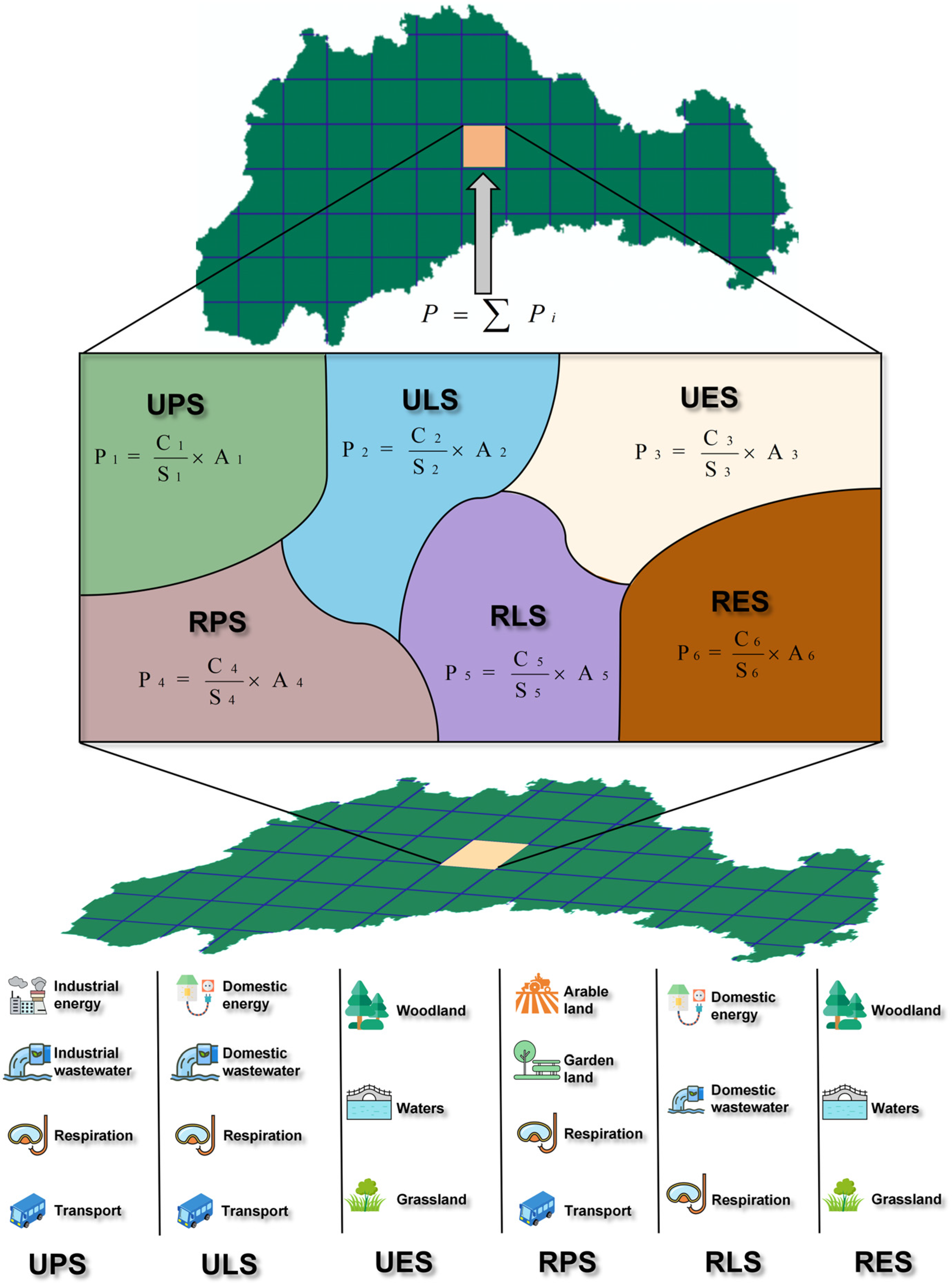
Figure 2. Spatial unit-based simulation framework for TSF carbon emissions distribution: UPS is urban production space; ULS is urban living space; UES is urban ecological space; RPS is rural production space; RLS is rural living space; RES is rural ecological space.
Land 14 01689 g002
Figure 3. TSFP of Qionglai City in 2020, 2025, and 2030: TSFP refers to territorial spatial functional patterns. (a) TSFP in 2020; (b) TSFP in 2025; (c) TSFP in 2030. UPS is urban production space; ULS is urban living space; UES is urban ecological space; RPS is rural production space; RLS is rural living space; RES is rural ecological space.
Land 14 01689 g003
Figure 4. Urban space expansion and driving factor contribution: UPS is urban production space; ULS is urban living space; UES is urban ecological space; RPS is rural production space; RLS is rural living space; RES is rural ecological space. (a) Spatial distribution of UPS in 2025; (b) Spatial distribution of ULS in 2025; (c) Spatial distribution of UES in 2025; (d) Spatial distribution of UPS in 2030; (e) Spatial distribution of ULS in 2030; (f) Spatial distribution of UES in 2030; ESPC is Environmental purification; PD is Population Density; TR is Topographic relief; HQ is Biodiversity maintenance; WC is Water supply; SC is Soil conservation; RND is Road network density; ET is Climate regulation; DPS is Proximity to public services.
Land 14 01689 g004
Figure 5. Temporal evolution of carbon emissions in Qionglai City from 2010 to 2030: UPS is urban production space; ULS is urban living space; UES is urban ecological space; RPS is rural production space; RLS is rural living space; RES is rural ecological space.
Land 14 01689 g005
Figure 6. Spatiotemporal variation of carbon emissions in Qionglai’s territorial space: (a) Carbon emissions in 2010; (b) Carbon emissions in 2012; (c) Carbon emissions in 2014; (d) Carbon emissions in 2016; (e) Carbon emissions in 2018; (f) Carbon emissions in 2020.
Land 14 01689 g006
Figure 7. Forecast of carbon emissions in the territorial space of Qionglai City for 2025 and 2030: (a) Carbon emissions in 2025; (b) Carbon emissions in 2030.
Land 14 01689 g007
Figure 8. Impact factor spatial distribution map: (a) Spatial distribution of GDP; (b) Spatial distribution of Secondary Industry Density; (c) Spatial distribution of Population Density; (d) Spatial distribution of Fuel Vehicle Density; (e) Spatial distribution of Temperature; (f) Spatial distribution of Net Primary Productivity (NPP).
Land 14 01689 g008
Figure 9. Spatial distribution of regression coefficients of impact factors: (a) Regression coefficients for GDP; (b) Regression coefficients for secondary industry density; (c) Regression coefficients for population density; (d) Regression coefficients for fuel vehicle density; (e) Regression coefficients for temperature; (f) Regression coefficients for Net Primary Productivity (NPP). Insets A, B, and C present enlarged views of the central, eastern, and western regions of Qionglai City, respectively.
Land 14 01689 g009
Figure 10. Urban expansion and spatial distribution of carbon emissions under scenario I: “RLS–UPS, RLS–UES, RLS–ULS, RES–ULS” represent the transition from the former function to the latter function, for example, “RLS-UPS” represents the transition from rural living space to urban production space. Scenario I represents urban expansion scenarios under historical evolution patterns. “<5” indicates territorial spatial units with carbon emissions less than 5 t; “5–10” indicates units with emissions between 5 and 10 t; “10–15” indicates emissions between 10 and 15 t; “15–20” represents emissions between 15 and 20 t; “>20” represents spatial units with carbon emissions greater than 20 t. (a) Urban expansion in 2025 under scenario I; (b) Spatial distribution of carbon emissions in 2025 under scenario I; (c) Urban expansion in 2030 under scenario I; (d) Spatial distribution of carbon emissions in 2030 under scenario I.
Land 14 01689 g010
Figure 11. Urban expansion and spatial distribution of carbon emissions under scenario II: “RPS–UPS, RPS–ULS, RPS–UES, RLS–UPS, RLS–ULS, RLS–UES, RES–ULS, RES–UES” represent the transition from the former function to the latter function, for example, “RPS-UPS” represents the transition from rural production space to urban production space. Scenario II represents urban expansion scenarios optimized under carbon neutrality targets. “<5” indicates territorial spatial units with carbon emissions less than 5 t; “5–10” indicates units with emissions between 5 and 10 t; “10–15” indicates emissions between 10 and 15 t; “15–20” represents emissions between 15 and 20 t; “>20” represents spatial units with carbon emissions greater than 20 t. (a) Urban expansion in 2025 under scenario II; (b) Spatial distribution of carbon emissions in 2025 under scenario II; (c) Urban expansion in 2030 under scenario II; (d) Spatial distribution of carbon emissions in 2030 under scenario II.
Land 14 01689 g011
Table 1. Data types and sources.
Data TypeData NameTime-Series
(Year)
ResolutionData Source
Raster dataDEM202012.5 m91 Visitor Assistant
Google satellite image202010 mhttps://developers.google.com/earth-engine/datasets (accessed on 19 January 2025)
Territorial space–function distribution map2009–202350 m Previous research datasets [49]
Temperature2000–20201 kmNational Tibetan Plateau/Third Pole Environment Data Center http://data.tpdc.ac.cn
(accessed on 19 January 2025)
Precipitation
Net primary productivity2000–2020500 mNational Earth System
Science Data Center
https://www.geodata.cn/data/index.html?word=NPP (accessed on 19 January 2025)
NDVINational Earth System
Science Data Center
https://www.geodata.cn/main/face_scientist?categoryId=&word=NDVI (accessed on 19 January 2025)
Vector DataAdministrative boundary20201:5000Sichuan Academy of Land Science and Technology
Land use status data2009–20231:5000Sichuan Academy of Land Science and Technology
Road Network Vector Data-OpenStreetMap
Panel dataNumber of pigs (head)2009–2023County levelQionglai Statistics Bureau
Number of cows (head)
Number of sheep (head)
Urban population (person)Township-level
Rural population (person)
GDP per capita (104 CNY/person)
Energyconsumption per 104 CNY of industrial output
(tce/104 CNY)
2009–2023City-levelChengdu Municipal Bureau of Statistics
Per capita electricity
consumption (kWh/person)
Per capita natural gas consumption (m3/person)
Per capita liquefied gas
consumption (kg/person)
Chemical oxygen demand (COD) in wastewater (t)2009–2023Provincial-levelChina Energy Statistical Yearbook
Table 2. Indicators of driving factors for urban spatial expansion.
Driving FactorMeasurement
Indicators
DescriptionUnit
Topography and LandformElevationVertical height of a surface point relative to the mean sea level.m
SlopeRatio of vertical rise to horizontal distance on the land surface.%
Topographic reliefMaximum relative elevation difference per unit area.m/km2
Natural
Environment
Water conservationThe ecosystem’s ability to purify, store, and supply freshwater.m3/raster
EvapotranspirationTotal volume of water released into the
atmosphere through plant transpiration.
m3/d
Environmental
purification service
capacity
The ecosystem’s self-purification capacity for water and air.-
Soil conservationIndex of the ecosystem’s ability to control erosion and maintain nutrient cycling.-
Habitat qualityComposite index for biodiversity maintenance and ecological sustainability.-
Transportation LocationRoad network densityRatio of total road length to the area of the evaluation unit.km/km2
Distance to public
services
Shortest feasible distance to key public service facilities (e.g., education, healthcare).m
SocioeconomicPopulation densityNumber of permanent residents per unit area.people/km2
Per capita GDPRatio of total GDP to the permanent population.104 CNY/person
Table 3. Carbon emission inventory for TSFs.
Territorial Space TypeTerrestrial
Ecosystems
Energy ConsumptionWastePopulation and LivestockOthers
UPS Industrial energy consumption, Service energy consumptionIndustrial wastewaterUrban population respirationTransportation land
ULS Urban residential energy
consumption
Domestic wastewaterUrban population respirationTransportation land
UESForest land, water bodies, grassland
RPSCropland, orchard land Livestock respiration, enteric
fermentation, and manure
Transportation land
RLS Rural residential energy
consumption
Domestic wastewaterRural population respiration
RESForest land, water bodies, grassland
Note: TSFs refer to territorial spatial functions; UPS is urban production space; ULS is urban living space; UES is urban ecological space; RPS is rural production space; RLS is rural living space; RES is rural ecological space.
Table 4. Indicators of driving factors for carbon emissions from urban expansion.
Driving FactorsDescriptionUnit
GDP per Unit AreaGDP generated per unit of territorial space area.104 CNY/hm2
Secondary Industry
Output Density
The output value of the secondary industry per unit of territorial space area.104 CNY/hm2
Population DensityNumber of residents per unit of territorial space area.persons/hm2
Number of fuel vehiclesNumber of fuel vehicles per unit of territorial space.vehicles/hm2
TemperatureAverage air temperature within a unit territorial space.°C
NPPNet primary productivity of vegetation per unit territorial space area.kgC/m2/year
Table 5. Qionglai City TFQS optimization results.
Type of Territorial Functions202020252030
First-LevelSecond-LevelArea (hm2)%Area (hm2)%Area (hm2)%
UrbanUPS501.600.36521.610.38536.810.39
ULS5258.953.825364.983.905474.753.98
UES334.180.24363.180.26374.190.27
RuralRPS59,600.5343.2859,631.4843.3059,652.5443.31
RLS9443.616.869135.606.638851.136.43
RES62,584.2945.4462,706.3145.5362,833.7445.62
Total137,723.16100.00137,723.16100.00137,723.16100.00
Note: TFQS refers to territorial spatial function quantity structure; UPS is urban production space; ULS is urban living space; UES is urban ecological space; RPS is rural production space; RLS is rural living space; RES is rural ecological space.
Table 6. Results of the GTWR model.
VariableMinimumMedianMaximumMeanPositive (%)Negative (%)
GDP per Unit Area0.24 0.38 0.44 0.37 100.00 0.00
Secondary Industry Output
Density
0.03 0.05 0.30 0.07 100.00 0.00
Population density0.06 0.04 0.09 0.03 92.28 7.72
Number of fuel
vehicles
0.10 0.04 0.09 0.03 82.41 17.59
Temperature0.33 0.03 0.13 0.02 82.07 17.93
NPP0.07 −0.04 0.02 −0.04 13.31 86.69
Table 7. Qionglai City TFQS optimization results under scenario II.
Type of Territorial Functions202020252030
First-LevelSecond-LevelArea (hm2)%Area (hm2)%Area (hm2)%
UrbanUPS501.600.36528.660.38 557.600.40
ULS5258.953.825333.603.87 5475.103.98
UES334.180.24441.300.32 480.600.35
RuralRPS59,600.5343.2859,451.7043.17 59,270.0643.04
RLS9443.616.868596.206.24 6164.504.48
RES62,584.2945.4463,371.7046.01 65,775.3047.76
Total137,723.16100.00137,723.16100.00137,723.16100.00
Note: TFQS refers to territorial spatial function quantity structure; scenario II refers to urban expansion scenarios optimized under carbon neutrality targets. UPS is urban production space; ULS is urban living space; UES is urban ecological space; RPS is rural production space; RLS is rural living space; RES is rural ecological space.
Table 8. Carbon neutrality pathways for urban expansion under different scenarios and design of implementation strategies.
Carbon Neutrality20252030
Scenario IScenario IIScenario IScenario II
QuantityCarbon EmissionsQuantityCarbon EmissionsQuantityCarbon EmissionsQuantityCarbon Emissions
Urban
expansion space (hm2)
155.056035.50208.743782.7135.987206.90208.886884.4
Optimization of urban green space vegetation types (hm2)7.36−349.8466.73−3170.288.89−422.2267.57−3210.09
Replacement of fuel vehicles with new energy vehicles (units)800−24.37800−24.371470−44.781470−44.78
Control of carbon emissions per unit of GDP (t/104 CNY)0.20−1010.580.21−588.050.15−396.700.15−1049.89
Purchase of carbon credits (104 CNY)32.34−4650.710.000.0044.11−6343.2017.94−2579.64
Note: In the carbon emission column, “+” indicates carbon emissions, while “−” indicates carbon storage. Scenario I represents urban expansion scenarios under historical evolution patterns; Scenario II represents urban expansion scenarios optimized under carbon neutrality targets.
Disclaimer/Publisher’s Note: The statements, opinions and data contained in all publications are solely those of the individual author(s) and contributor(s) and not of MDPI and/or the editor(s). MDPI and/or the editor(s) disclaim responsibility for any injury to people or property resulting from any ideas, methods, instructions or products referred to in the content.