Article

Analysis of Carbon Storage Changes in the Chengdu–Chongqing Region Based on the PLUS-InVEST-MGWR Model

1
College of Resource, Sichuan Agricultural University, Chengdu 611130, China
2
College of Economics, Sichuan Agricultural University, Chengdu 611130, China
*
Author to whom correspondence should be addressed.
Land 2025, 14(8), 1651; https://doi.org/10.3390/land14081651
Submission received: 6 June 2025 / Revised: 1 August 2025 / Accepted: 12 August 2025 / Published: 15 August 2025

Abstract

Urbanization-induced ecological problems have affected China’s urban agglomerations since the beginning of rapid economic growth. The InVEST model can be used to study how land use changes affect carbon storage, while land simulation models help project future land use trends and assess the impact of policies on land use, thereby predicting future carbon storage. This study constructs a PLUS-InVEST-MGWR model, corrects carbon storage values in ArcGIS, and thereby analyzes its heterogeneity by MGWR. The economic value of carbon storage is calculated as well. The main findings are as follows: (1) The downward trend of carbon storage in the Chengdu–Chongqing region will continue but slow down to some extent, and only the ecological security scenario can prevent it. (2) In 2015, China’s social cost of carbon (SCC) was CNY 60.83 per ton, with a discount rate of 6.468%, while the economic value of carbon storage (EVCS) in the Chengdu–Chongqing region was CNY 289.516 × 10⁹. (3) Spatial correction of carbon storage is crucial for enhancing the goodness-of-fit and result accuracy of the MGWR model, as the absence of such correction would significantly degrade its performance. The revised InVEST model enables rapid quantification of carbon storage’s spatial heterogeneity.

1. Introduction

Carbon storage refers to the amount of carbon contained in a carbon pool, and its estimation is essential for protecting ecosystem carbon sinks and related policy formulation [1]. Carbon storage is not only crucial for ecosystem functions, but also directly affects the stability and balance of the global carbon cycle [2]. As a substantial global carbon pool, terrestrial ecosystems play a fundamental role in climate change dynamics. They are key components of the global carbon sink, facilitating CO2 absorption and mitigating the greenhouse effect, thereby contributing to the global carbon cycle [3,4]. Therefore, carbon storage has been identified as a pivotal ecosystem service in the United Nations’ 2005 Millennium Ecosystem Assessment Report [5].
In recent years, developments in technology have resulted in a significant enhancement of the methods available for the study of carbon storage. Estimation approaches include field surveys, remote sensing, and model-based simulations [6]. Extensive field studies and modeling efforts have enabled researchers to ascertain unit carbon storage values for various land use types, thereby facilitating the construction of carbon pool tables. Among these models, CASA, LPJ-GUESS, FORCCHN DNDC, and InVEST are the most widely used. With the rapid advancement of remote sensing technology, an increasing number of researchers have employed a combination of remote sensing and modeling approaches to study carbon storage [7,8]. The InVEST model is particularly notable for its ease of use, flexibility, minimal parameter requirements [9], extensive analytical capabilities, and ability to simulate the spatial and temporal distribution of carbon storage on a large scale [10]. Consequently, this model is well-suited for integration with remote sensing and is frequently utilized in ecosystem service assessments. Anthropogenic land use has a profound impact on carbon storage in terrestrial ecosystems [11,12]. Social and economic factors shape land-use decisions and resource management practices, thereby impacting carbon storage dynamics [13]. Hence, dynamic Land Use and Land Cover Change (LUCC) simulation is considered a key factor affecting carbon storage [14,15] and the carbon cycle [16]. As a result, many studies have employed the InVEST and LUCC models to analyze carbon storage and its changes [9,17]. Some researchers, such as Zhou et al. [18], quantified the economic value of carbon storage after calculating carbon storage estimates. They applied a discount rate of 10% to 12%, following the recommendation of the Asian Development Bank and the InVEST software (v3.14.2). However, this discount rate of China has declined to 8% since 2006 [19]. Estimates through this approach are inaccurate.
Following the launch of the LUCC Scientific Research Program by the International Geosphere-Biosphere Program (IGBP) and International Human Dimensions Program on Global Environmental Change (IHDP) in 1995, numerous scholars have conducted extensive research on LUCC [20]. LUCC simulations are divided into two parts: area and spatial distribution prediction of land use types. Given that the Markov chain can perform scenario analysis and offer good accessibility, the majority of studies use this method to predict land use area. A variety of spatial simulation models have been developed to simulate dynamic land use patterns [21,22], including Cellular Automata [23,24], Logistic-CA [25], ANN-CA [26], Dyna-CLUE [27,28,29], CLU Mondo [30], FLUS [31], and PLUS [32], among others. Among these simulation models, the recently developed PLUS model retains the advantages of adaptive inertial competition and the roulette competition mechanism [33] while determining the development potential of each land use type through the Random Forest (RF) algorithm [34]. Consequently, the PLUS model’s accuracy is widely recognized by scholars. In addition to directly predicting future land use patterns, LUCC models are also employed for multi-scenario simulations. In such studies, researchers define different land use demands for each scenario to simulate different development scenarios shaped by government policies [35,36]. In LUCC simulations, urban expansion is usually the most prominent change, especially in regions experiencing rapid urbanization. The rapid growth of urban areas has resulted in significant changes in land use and landscape patterns [37,38], leading to a series of environmental challenges directly linked to urbanization [39,40], particularly its impact on carbon storage. Hence, numerous studies have analyzed the impact of urban sprawl on carbon storage [41,42,43,44,45]. For instance, Mendoza-Ponce et al. [46] suggested that by the end of the 21st century, Mexico could restore its total carbon storage to 1985 levels by reducing deforestation rates and increasing natural vegetation coverage. Nie et al. [13] explored the driving factors behind urban expansion and its impact on carbon storage using the Geodetector method. Peng et al. [47] found a negative correlation between ecological risk and carbon storage in the Wuhan metropolitan area. However, the majority of these studies have not been able to develop regionally specific scenarios based on comprehensive and holistic analyses when projecting future land use.
Current research on spatial heterogeneity analysis of carbon storage remains limited. Existing studies primarily utilize remote sensing data [48,49], the GEOERC dataset [50], or the InVEST model [13,51,52,53,54,55] to estimate carbon storage for multi-scale geographically weighted regression (MGWR) analysis. Of these, the InVEST model is most commonly used. For example, Jia et al. [56] report the relationship between carbon density and sample scale, Qin et al. [13] compared results of MGWR with those of Geodetector, and Lai et al. [54] utilized the CatBoost method to rank driving factors. However, because the InVEST model assigns fixed carbon storage values to each land use type, it is incompatible with heterogeneity analysis models. This study compares heterogeneity analyses before and after spatial correction, thus demonstrating the necessity of spatial correction for such analyses.
This study aims to quantify multi-scenario land use change impacts on carbon storage in the Chengdu–Chongqing region between 1990 and 2050. Its general objective is to identify optimal pathways for carbon-neutral land planning through an integrated assessment framework. Four specific objectives are pursued chronologically: first, simulating future land-use patterns via the PLUS model; second, correcting the InVEST model and assessing carbon storage dynamics; third, evaluating economic value using a China-specific discount rate; fourth, uncovering spatial drivers of carbon storage via MGWR. Results demonstrate that ecological-focused scenarios uniquely prevent carbon loss despite urbanization pressures (Figure 1).

2. Materials and Methods

2.1. Study Area

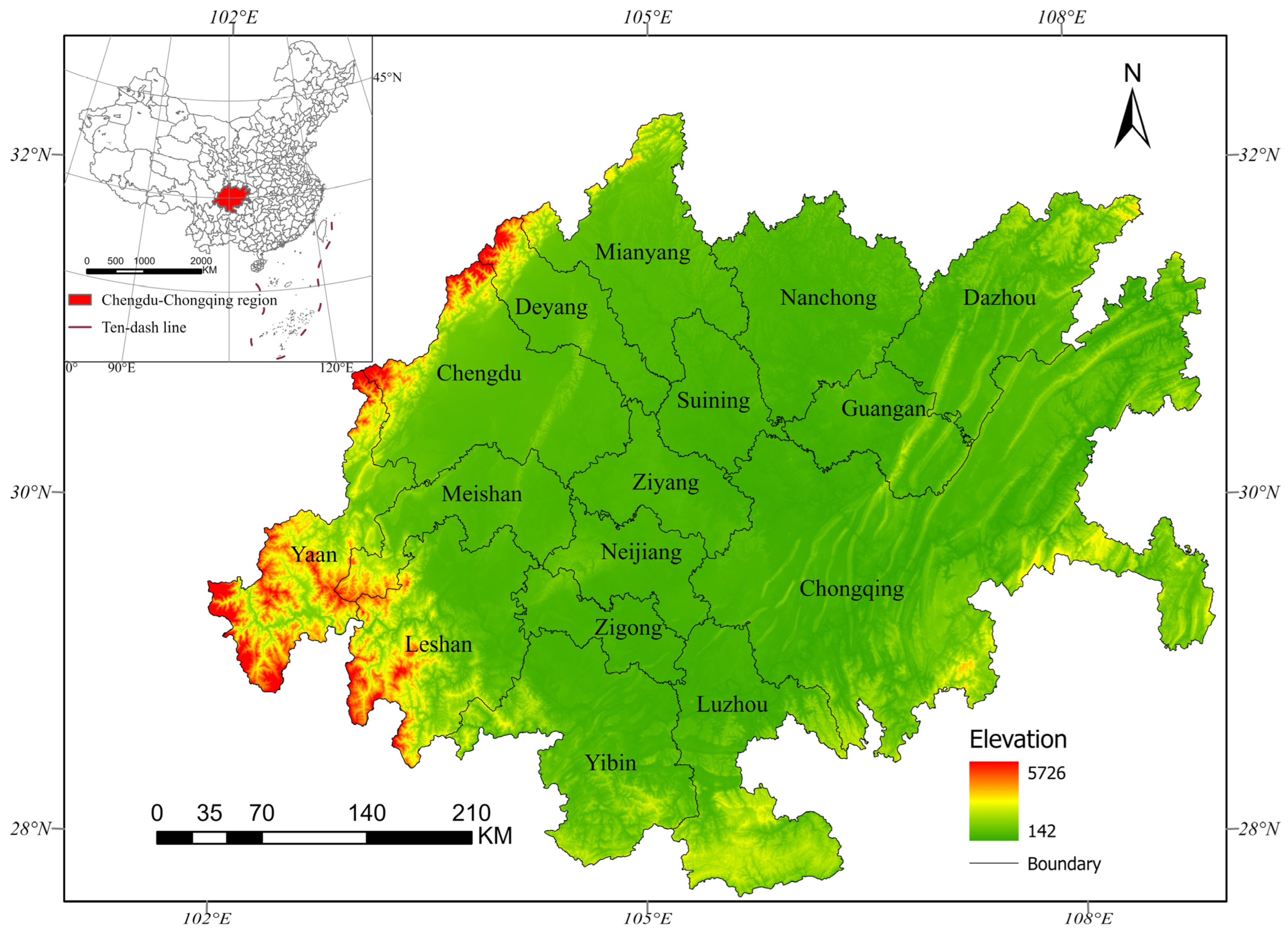
The Chengdu–Chongqing region is located in southwestern China, in the upper reaches of the Yangtze River, serving as an important hub connecting eastern and western China. It encompasses Chongqing’s 27 counties and portions of the Kaizhou District and Yunyang County, along with 15 cities in Sichuan Province [57] (Figure 2). In 2020, the Chengdu–Chongqing region had a population of approximately 115.729 million and a GDP of CNY 7.36 trillion, accounting for around 8.02% of the national population and 7.24% of the national GDP, respectively [58]. The region is located in the Upper Yangtze River Economic Belt [59] and encompasses multiple large-scale ecological zones, including the Upper Yangtze River Ecological Barrier Area, Giant Panda National Park, and Three Gorges Reservoir Area Ecological Conservation Zone, serving as a critical provider of ecological services in China.

2.2. Data Sources and Processing

There are two categories of data used for land use change scenario simulation: land use data and driving factors of land use and land cover change. The land use data were obtained from the Resource and Environmental Science Data Platform, with an accuracy of no less than 9ter, for construction land, and unused land. In the selection of driving factors, data accuracy and availability were prioritized, while simplicity and prevention of multicollinearity were also considered to ensure the optimal performance of the MGWR model. Based on an empirical analysis and previous Chinese literatures of land use change in the study area, 11 driving factors were selected: elevation, slope, annual precipitation, annual average temperature [60], distance to rivers, distance to railways, distance to highways, distance to roads, distance to administrative centers, GDP density, and population density (Table 1). All data were projected to the Krasovsky_1940_Albers coordinate system, removed nulls via the raster calculator, and resampled to a resolution of 300 m × 300 m. Annual precipitation and annual average temperature were also used to calculate carbon storage.

2.3. Methods

Land use changes between 2010 and 2020 were derived from the PLUS model. The map of these changes, in conjunction with the processed driving factor data, was integrated into the Land Expansion Analysis Strategy (LEAS) module to generate LEAS. The 2010 land use map and LEAS were then used in the cellular automata (CA) based on the Multiple Random Seeds (CARS) module to simulate the 2020 land use map. Then, the simulated map was compared with the actual 2020 land use map for model validation. Model parameters were continuously adjusted to enhance simulation accuracy. Following the successful completion of the test, the parameters were maintained constant, and the 2020 land use map and LEAS were utilized to predict future land use.
The carbon density table was compiled based on previous research findings. This table, along with the simulation results from the PLUS model, was input into the InVEST software to generate a carbon storage map. The correction factor for each patch was then calculated in GIS to generate a corrected carbon storage map. Finally, the processed data were exported for economic value calculation and MGWR analysis.

2.3.1. PLUS Model

The PLUS model is a raster-based, patch-generating land use simulation model designed to identify underlying drivers of land use change and assess their differing contributions. It incorporates a rule-mining framework derived from the LEAS and CARS [32]. LEAS indicates the likelihood of different land use types occurring on patches by extracting the spatial characteristics of land use expansion and analyzing driving factors between two periods. The model uses the RF algorithm to sample land use expansion areas and associated driving factors, calculates the probability of land use change, and determines the contribution of each driving factor. The comprehensive probability of land use change is then obtained through an adaptive inertia competition mechanism based on a roulette wheel selection approach. By inputting LEAS results and an initial land use map, the PLUS model generates future land use patterns through CARS. Future land use is determined by combining the generation of random patches, a transition matrix, and a threshold-decreasing mechanism [61]. Due to the limitations of development potential, the PLUS model automatically produces simulated results [10]. It effectively optimizes land use layout and provides a more accurate simulation of various land use patch changes [62].

2.3.2. Markov Chain

A Markov chain is used to predict future land use demand. It is a memoryless process in which the future state depends only on the current state and the transition step size, independent of any prior states [63,64]. It also reflects the idea that the present encapsulates past influences, allowing future predictions based on current conditions, which is consistent with the characteristics of land use change. The Markov chain predicts future land use by calculating the Markov matrix. This matrix is a singular probability matrix, where the sum of each column vector equals 1 [65]. The area of the six land use types is represented as a 6 × 1 land use matrix, which is then left-multiplied by the Markov matrix to compute the full probability of dynamic changes in each land use type. The formula is as follows:
Aa x1 = x2
where x1 represents land use at the previous time point, x2 denotes land use at the future time point, A indicates the Markov matrix, and a refers to the time interval (in years) between the two points.
The value of Aa can be calculated using the Markov module in the IDRISI 18.0 software package [66,67] or in the PLUS software (v1.4). The matrix A is initially calculated in MATLAB R2023a, after which it is adjusted, and Aa is recalculated under different scenarios.

2.3.3. Scenarios and Parameters

Based on a comprehensive assessment of regional resource endowments, comparative advantages, and different development objectives, different scenarios were established under various land use planning and policy frameworks [36,68,69]. Three key development objectives are considered: economic growth, food production, and ecological conservation. Accordingly, three basic scenarios are defined: business as usual (BAU), cropland protection (CP), and ecological security (ES) [70,71]. Under the BAU scenario, the development of the study area will maintain the trends of the past 10 years. Under the CP scenario, the approval for converting cropland will become more stringent, making it more difficult to occupy agricultural land. Meanwhile, land consolidation and rehabilitation will be conducted more frequently. Under the ES scenario, ecological protection policies, such as the Opinions on Promoting High-Quality Development of Returning Farmland to Forests and Grasslands, will be further promoted. Moreover, the successful experience of Chengdu in developing a new type of park city is expected to be expanded throughout the Chengdu–Chongqing region.
The Chinese government has set a target to reach peak carbon emissions by 2030 and achieve carbon neutrality by 2060. He et al. [72] pointed out that achieving this goal requires reaching net-zero emissions by 2050. The Construction Plan Outline for the Chengdu–Chongqing Economic Circle explicitly states that the Chengdu–Chongqing region must prioritize ecological considerations and pursue green development. Therefore, the Chengdu–Chongqing region may be required to place ecological development as the top priority to meet the demands of carbon neutrality after 2030. Regardless of the development scenario adopted during 2020–2030, a transition to the ES scenario will likely become imperative by 2030.
Hence, five scenarios were developed for the Chengdu–Chongqing region, including BAU, CP, ES, BAU-ES, and CP-ES. Land demand, transition matrices, and neighborhood weights for each scenario were then input into the simulation models accordingly.
(1)
Land demand
Land use demand for 2030 and 2050 under different scenarios is calculated using the Markov chain model based on land use data from 2010 to 2020.
In the BAU scenario, the probability matrix will remain consistent with that of the 2010–2020 period.
In the CP scenario, the probability of converting cropland into forest, grassland, water, construction land, and unused land will be reduced by 10%, 30%, 20%, 40%, and 80%, respectively. Conversely, the probability of converting forest, grassland, and construction land to cropland will increase by 10%, while unused land will be 50% more likely to be converted to cropland.
In the ES scenario, the probability of converting forest, grassland, and water to cropland, construction land, and unused land will decrease by 20%, 30%, and 30%, respectively. Meanwhile, the probability of converting cropland, construction land, and unused land to forest will increase by 20%. Additionally, the probability of converting cropland to construction land will be reduced by 25% in order to prevent excessive cropland reduction.
(2)
Transition matrix
The transition matrix determines whether land use conversion is possible, with values of 0 and 1, indicating impossible and possible conversion, respectively. Analyzing historical land use changes from 2010 to 2020 in the study area reveals that all land use conversions are possible. However, during the debugging process of the PLUS model, achieving the target water area proved challenging. To improve model accuracy, water areas were restricted from converting to any land type except cropland. This adjustment enhances the model’s validation accuracy.
(3)
Neighborhood weights
Neighborhood weights define the relative probability of one land use type converting to another, ranging from 0 to 1. A higher neighborhood weight value indicates a greater likelihood of conversion to a specific land type. These values are adjusted during the calibration of the model. Through experimentation with different weight adjustments, the method recommended by Xun Liang [32] in the PLUS software user guide was found to produce the most accurate simulation results. In this way, neighborhood weights are determined by calculating the proportion of the expansion area of each land type relative to the total expansion area [73].

2.3.4. Kappa Test

The Kappa index is a test method proposed by Cohen [74] to assess whether the classification results of remote sensing images are consistent by establishing an error matrix comparing land use data with image classification results. Since land use maps are categorical datasets, the Kappa index can be used to measure the agreement between two maps. Therefore, it is frequently used for accuracy assessment of remote sensing image classifications [75,76] and spatial simulation model results [77,78,79]. The Kappa coefficient is calculated as follows:
O A O = ( k = 1 n O A k k ) / N K a p p a = O A O O A E 1 O A E
where O A O represents the overall accuracy (OA) of the classification, indicating the proportion of the simulation result that is consistent with the land use data for each random sample; O A E indicates the proportion of agreement expected by chance; n denotes the total number of land use types, N is the total number of samples; and O A k k indicates the number of correctly classified samples for the kth land use type. The Kappa coefficient ranges from −1 to 1, with higher values reflecting greater model accuracy [79,80]. A Kappa value ≥ 0.81 indicates that the model has achieved a very high level of accuracy [74,81,82].
The Kappa test is used to validate the accuracy of the model. Given that a simulation step of 10 years has been selected, this study applies the 2010 land use map to simulate the 2020 land use map. During the 2010–2020 period, a total of 179,130 patches underwent change, accounting for 8.72% of the total number of patches. The proportion of converted patches exceeded 5%, effectively avoiding the false impression of accuracy that can arise from high Kappa scores in models with minimal land use change. The OA in this study is 91%, and the Kappa coefficient is 0.83, indicating that the model achieves satisfactory accuracy.

2.3.5. Carbon Storage Assessment

The InVEST model is widely recognized as an accurate method for assessing carbon storage. According to this model, most existing carbon storage in the environment is attributed to four primary carbon pools: aboveground carbon density, belowground carbon density, soil carbon density, and dead organic carbon density [18]. The total carbon storage is calculated as follows:
C t o t a l   =   [ C i _ a b o v e + C i _ b e l o w + C i _ s o i l + C i _ d e a d · A i ]
where C i _ a b o v e , C i _ b e l o w , C i _ s o i l , and C i _ d e a d represent the carbon densities of aboveground biomass, belowground biomass, soil, and dead organic matter for the i-th land use type, respectively; C t o t a l denotes the total carbon storage in the study area, i indicates the carbon density of the i-th land use type in the region; and Ai refers to the total area of the i-th land use type.
The carbon density used in this study is obtained from China’s National Ecological Science Data Centre [83], as shown in Table 2. Since the carbon density coefficient varies with climate change, soil properties, and land use, it differs across regions. Hence, the value of the selected region needs to be adjusted to more accurately estimate carbon storage [84]. Carbon density is correlated with precipitation and temperature, with precipitation showing a significant positive correlation [85]. The formulas studied by Alam [86] are used to adjust the precipitation factor, while the average temperature factor is corrected using formulas from Giardina et al. [87]. These two formulas have been widely recognized by Chinese scholars and adopted to study diverse regions across China [13,17,88]. The correction coefficients are calculated as follows:
C s p   =   3.3968   ×   P   +   3996.1 C B P   =   6.7981 e 0.00541 P C B T   =   28   ×   T   +   398
where C s p indicates the soil carbon density under the influence of annual average precipitation; C B P and C B T represent the carbon densities of aboveground biomass, belowground biomass, and dead organic matter under the influence of annual precipitation and annual average temperature, respectively. P and T denote the average annual precipitation (mm) and average annual temperature (°C) for the study period, respectively. The values of these three parameters for the study area and China were calculated, and the correction factor was computed according to the following equation:
K B   =   C B P C B P   ×   C B T C B T K S   =   C S P C S P
where K B denotes the overall correction coefficient of aboveground biomass, belowground biomass, and dead organic matter; K S indicates the correction coefficient for soil carbon density; C′ and C″ refer to the carbon densities of the study region and the national average, respectively. The resulting ratio serves as the correction coefficient.
To better capture the influence of urban expansion on carbon storage, the annual precipitation and average temperature from 1990 to 2020 are used to calculate these coefficients in GIS. These coefficients are then applied as correction factors for carbon storage across all studied years.

2.3.6. Assessment of Economic Value of Carbon Storage

The discount rate directly affects conclusions on climate change analysis and corresponding policy responses. With discount rates of 4.5% and 6.6%, SCC in 2015 was USD 16.35/tC and USD 9.2/tC, respectively [89]. At present, China still uses a fixed discount rate for measuring public investment. In this study, the discount rate is estimated through financial synthesis calculations and proportional relationship analysis. The treasury yields of long-term national debt issued by the Chinese government in 2015 are used to evaluate the discount rate. The formula is as follows [90]:
P   =   t     =     1 T [ C F ( 1   +   R ) t   +   F V ( 1   +   R ) t ]
where P represents the price of the bond, R denotes the yield to maturity of the bond (which serves as the discount rate), T indicates the bond term, FV refers to the face value of the bond, and CF represents the annual coupon payment.
After collecting treasury yields data for long-term national debt, the discount rate for public investment is estimated at 6.468%. By employing a straight-line method to fit the discount rate with its corresponding value in Tian’s result, the SCC in China in 2015 was determined to be USD 9.6/tC with a discount rate of 6.468%. The exchange rate of USD to CNY in 2015 was 1:6.336, indicating that the SCC in China in 2015 was CNY 60.83. Due to the complexity of the dynamics affecting SCC, EVCS of the study area for 2020, 2030, and 2050 is calculated using the SCC from 2015.

2.3.7. Multiscale Geographically Weighted Regression

Geographically weighted regression (GWR) is an advanced form of ordinary least squares (OLS) that serves as a localized modeling tool, enhancing global regression models by optimizing coefficients for individual geographic units [91,92,93]. This approach offers insights into spatial variations within data [94]. The GWR model is formulated as follows:
y i   =   j   =   1 k β j ( u i , v i ) x i j   +   ε i
where ( u i , v i ) represents the spatial location of point i, β j ( u i , v i ) denotes the locally calculated coefficients for the explanatory variable x i j at position i, and ε i refers to the residual at point i.
Multiscale geographically weighted regression (MGWR) is an improved version of GWR. In MGWR, each regression coefficient βj is estimated based on local regression with variable-specific bandwidths, which differs from classical GWR, where all variables share the same bandwidth. This allows analysts to more accurately understand and characterize spatial patterns in the data and to identify key influences at different scales [95]. Bandwidths were optimized by Golden Section Search with the goal of minimizing the Akaike Information Criterion with correction (AICc) value. The formula is as follows:
A I C c m i n     =     2 n   l n σ ^   +   n   l n 2 π   +   n [ n   +   t r ( S ) n     2   t r ( S ) ]
where tr(S) represents the trace of the bandwidth matrix, σ ^ represents standardized residual.

3. Results

3.1. Multi-Scenario Simulation Results

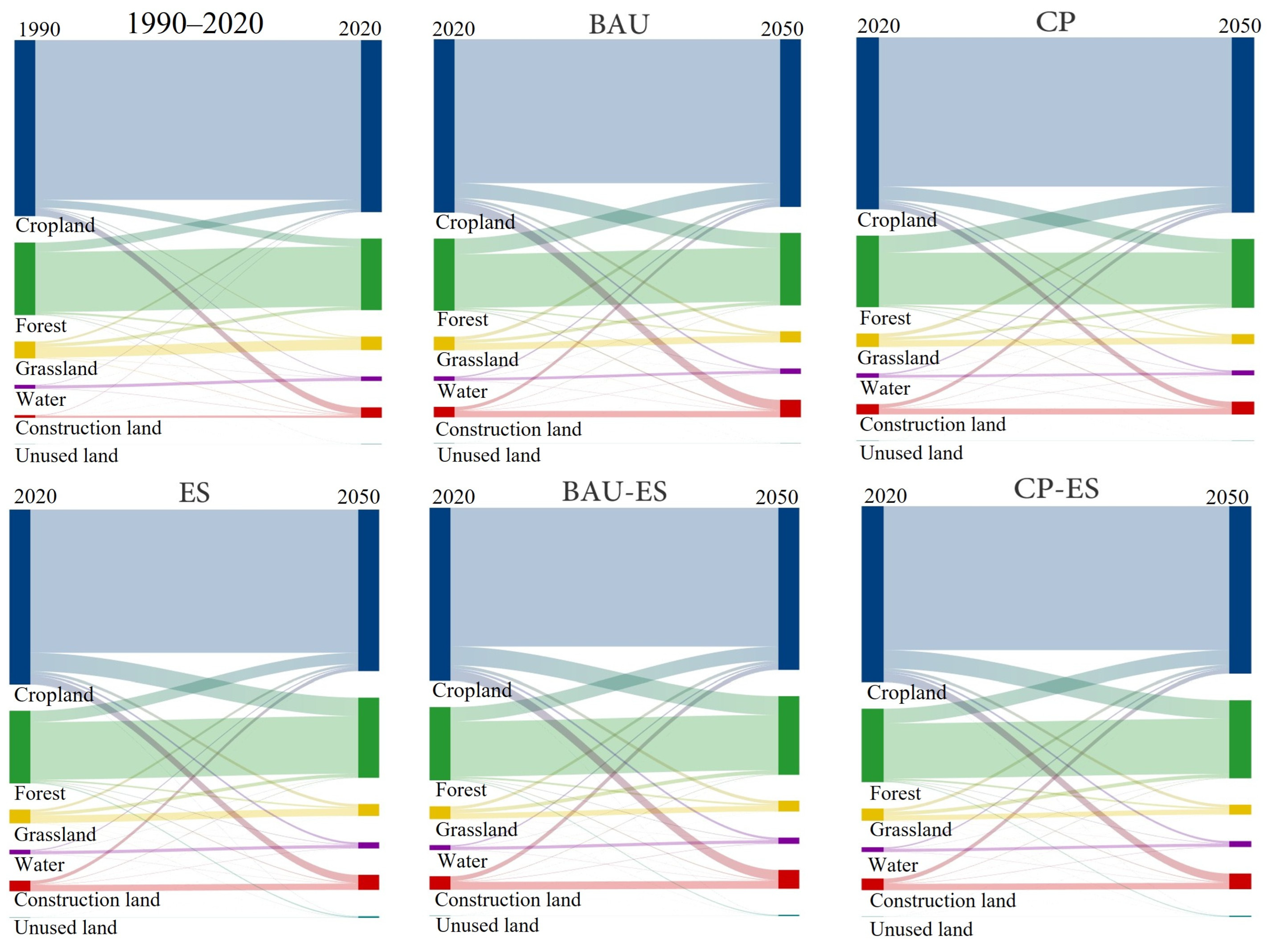
In the Chengdu–Chongqing region, cropland is the dominant land use type, accounting for 50% of the total area, followed by forest at 26%. Forest and grassland are mainly distributed in the southwestern and eastern peripheral mountainous areas, while cropland and construction land are mainly distributed in the flat central plain and the eastern low mountain and hilly areas. Through calculations, Sankey diagrams were used to visualize historical land use changes and those projected under different scenarios from 2020 to 2050 (Figure 3).
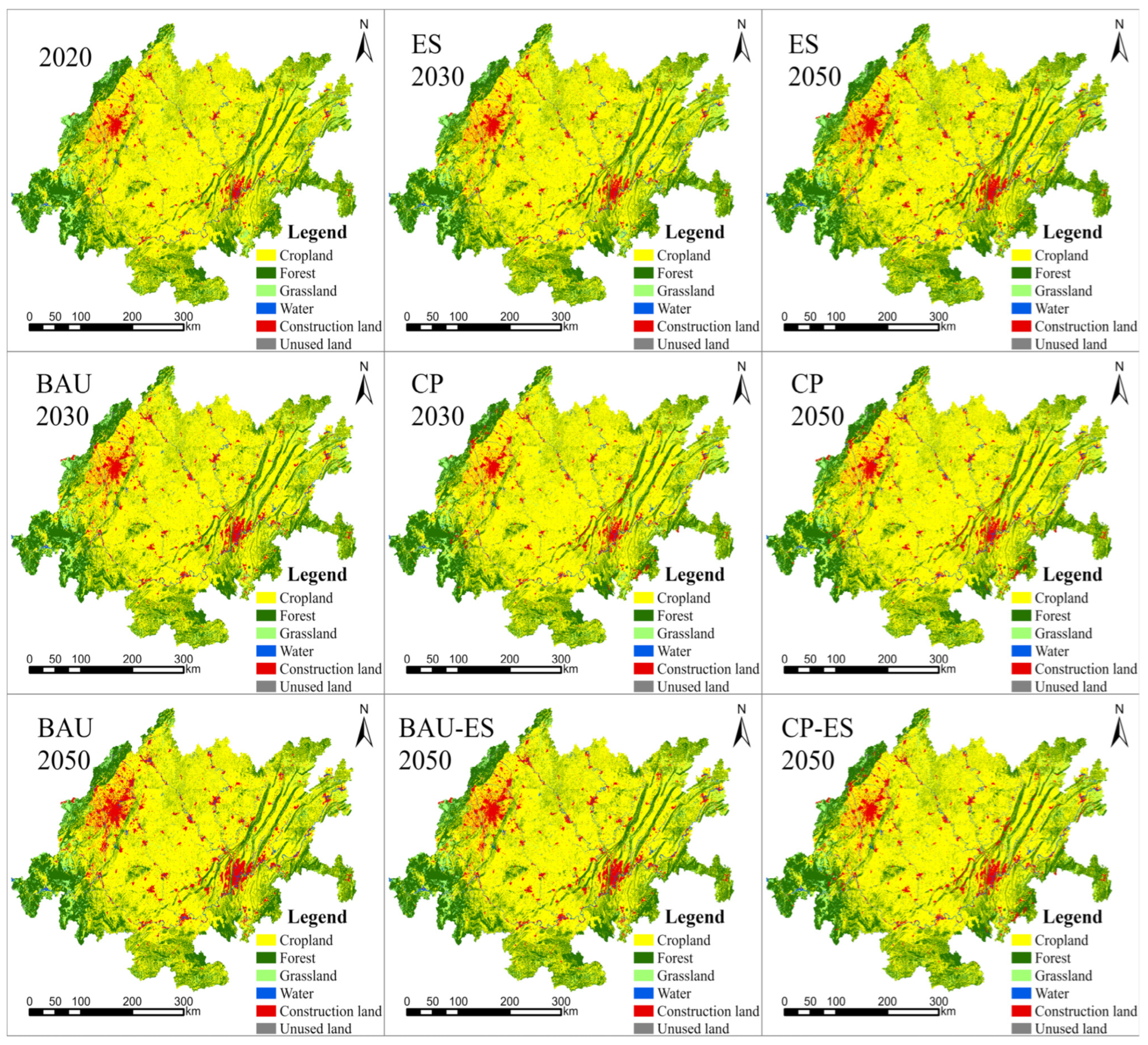
The simulation results across all five scenarios show that urban agglomeration in the Chengdu–Chongqing region will continue, showing a distinct dual-core structure. Chengdu and Chongqing serve as the primary development hubs, with most newly added construction land concentrated in these two cities. Land use changes predominantly occur in relatively flat areas, where the expansion of construction land leads to the conversion of substantial cropland, forest, and grassland. Cropland, in particular, undergoes significant conversion into construction land. The ecological space in the Chengdu–Chongqing region follows a “double circle” distribution pattern, characterized by a small circle in the central areas and a large one in the surrounding areas. There are notable increases and decreases in the number of water patches, with the majority of these changes occurring alongside existing rivers (Figure 4).
Only in the BAU scenario in 2050 does a substantial amount of construction land emerge in rural areas with minimal infrastructure and little to no prior development. This indicates an increase in urbanization and economic development in the countryside. In contrast, the expansion of construction land exhibits a distinctive mode of operation in the CP and CP-ES scenarios. Analyzing the distribution of construction land in 2020 reveals that most land near urban agglomerations consists of cropland. These high-quality croplands will be extensively converted into construction land, which is consistent with historical trends. However, the rigorous cropland protection policies implemented in the CP and CP-ES scenarios have significantly reduced such conversion near existing built-up areas. Instead, construction land expansion mainly occurs through the conversion of forested areas. From a spatial perspective, new construction land in 2020 remains concentrated near railways, highways, and roads. However, at the local level, the existing transportation infrastructure is insufficient to support the effective utilization of these new construction sites. Consequently, additional infrastructure development will be necessary to accommodate the anticipated demand for construction land.

3.2. Changes in Carbon Storage

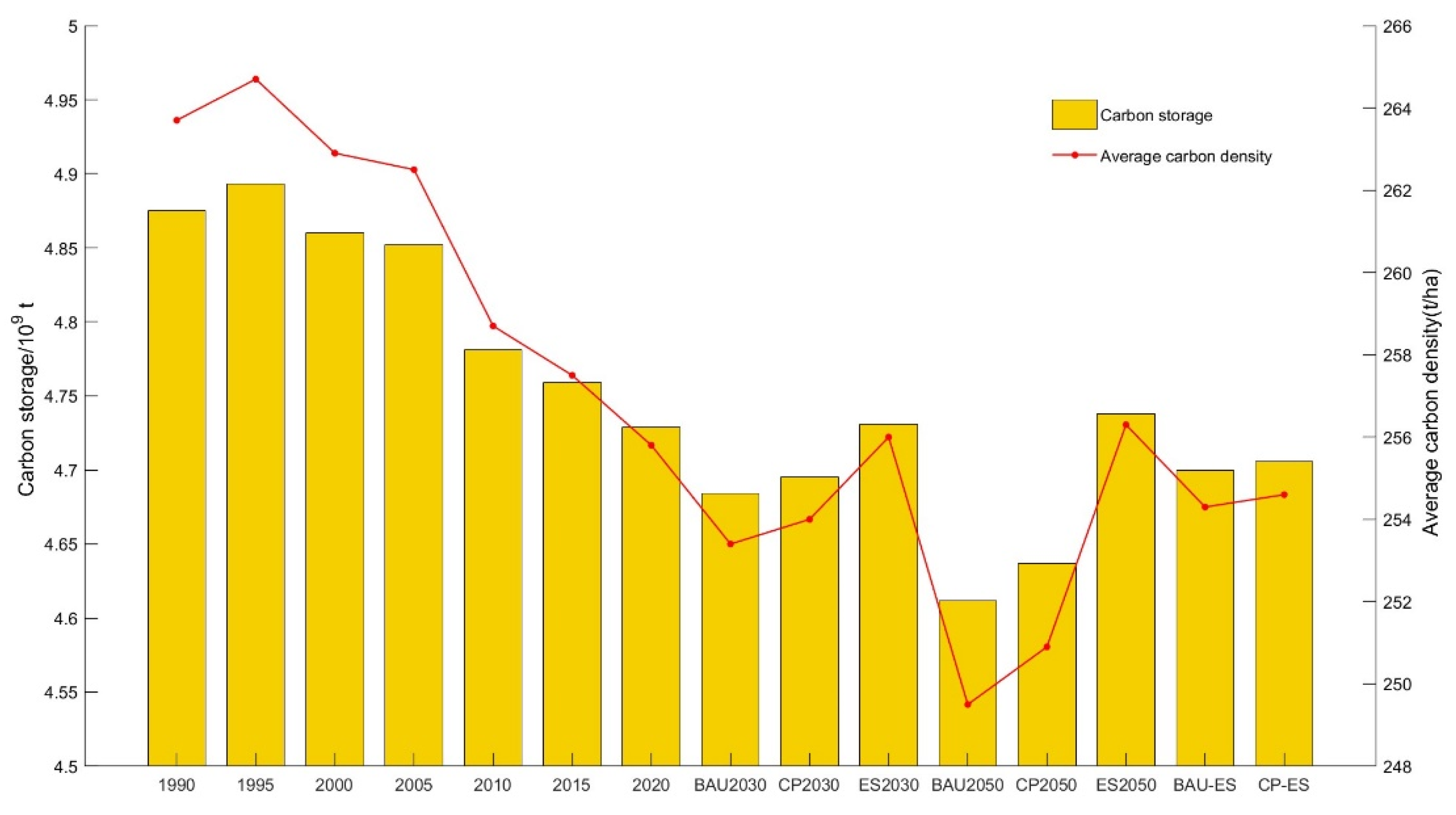
The general trend of carbon storage over the past 30 years was calculated, using a step length of 5 years. Between 1990 and 2020, carbon storage declined from 4874.91 × 106 t to 4728.85 × 106 t. It peaked in 1995 before entering a continuous downward trend, though the rate of decline moderated after 2010 (0.64% from 2015 to 2020). In 2030, carbon storage is projected to be 4684.04 × 106 t under the BAU scenario, 4694.7 × 106 t under the CP scenario, and 4731.46 × 106 t under the ES scenario. By 2050, across all scenarios, the highest projected carbon storage is 4737.73 × 106 t under the ES scenario, while the lowest is 4612.05 × 106 t under the BAU scenario (Figure 5). Carbon storage under the BAU, CP, BAU-ES, and CP-ES scenarios is expected to decrease by 2.47%, 1.93%, 0.6%, and 0.47%, respectively, compared to the baseline. Under the BAU scenario, carbon storage is projected to decrease by 0.41% every five years, indicating a slowing reduction trend. In contrast, under the ES scenario, carbon storage is expected to increase by 0.19%, suggesting that this scenario is the most conducive to carbon growth, which is consistent with findings from previous studies [47,96,97].
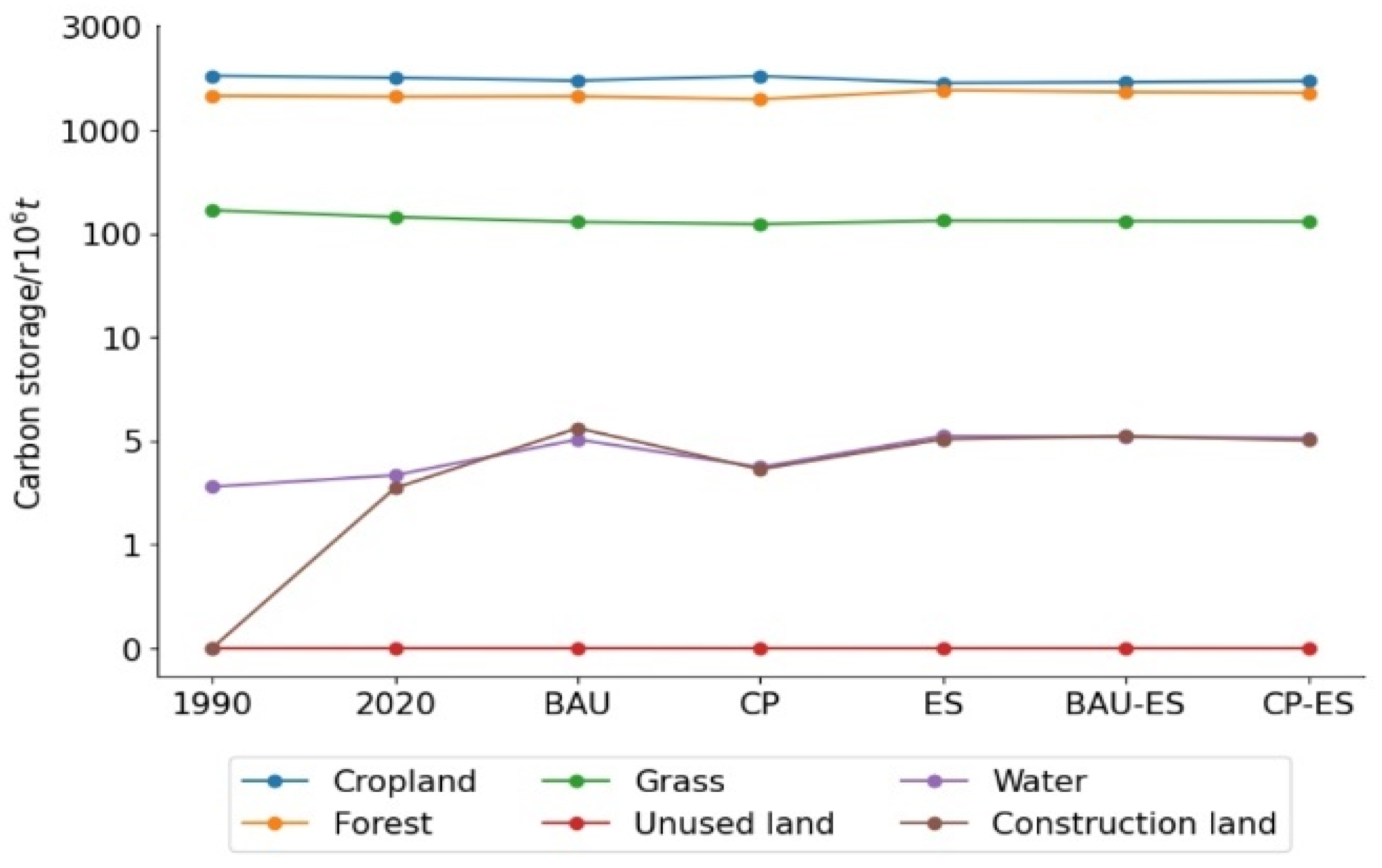
Figure 6 illustrates the dynamic components of carbon storage. Due to its numerical superiority, cropland is the top contributor to carbon storage. Forests, despite their smaller area, provide a substantial quantity of carbon storage due to the significant ecosystem services they provide. Grassland also plays a notable role in carbon storage. In 2020, cropland, forest, and grassland contributed 52.96%, 41.38%, and 5.47%, respectively. Driven by China’s implementation of a water protection policy, carbon storage in water has been steadily increasing. Due to urban expansion, carbon storage in construction land increased rapidly, from 0.96 × 10⁶ t to 3.72 × 10⁶ t, largely at the expense of cropland and grassland carbon storage.
Figure 7 shows the spatial changes of carbon storage in 2030 and 2050 across five scenarios, revealing a strong spatial overlap between carbon storage loss and urban expansion.
Despite the implementation of ecological protection measures, a significant increase in carbon storage within the Chengdu–Chongqing region is unlikely. This is primarily due to the ongoing trend of extensive urban expansion, which remains difficult to reverse. Therefore, it is necessary for the region to adopt policies aimed at reducing carbon emissions from newly developed cities, contributing to the goal of carbon neutrality.

3.3. Impacts of Urban Expansion on Carbon Storage

The contribution rate of urban to carbon loss (CR) was defined as the proportion of carbon storage reductions due to urban expansion to the total carbon storage reductions in the study area and is calculated in Table 3. Between 1990 and 2020, the Chengdu–Chongqing region received considerable policy support and experienced rapid urbanization, particularly after 2000, while carbon storage declined rapidly by 144.42 × 10⁶ t. Under the BAU scenario, urbanization advances steadily, but at a naturally slowing pace. In addition, the policy of returning cropland to forest remains in effect. Consequently, carbon storage declines at a slightly slower rate than in the past 30 years, although the proportion of carbon loss caused by urban expansion increases. In all other scenarios, urban expansion is effectively curbed. Under the CP scenario, urban expansion is the most restricted, totaling only 172,665 ha. However, considerable conversion of forest and grassland to cropland and construction land under the CP scenario results in a higher overall carbon storage loss compared to the ES, BAU-ES, and CP-ES scenarios. As a result, the CR is the lowest in this scenario. This reflects the fact that agricultural intensification has a significant reducing effect on carbon storage. Under the ES scenario, urban expansion predominantly occurs on cropland rather than forest or grassland, resulting in the lowest carbon storage loss due to urban expansion. The significant expansion of forest land ensures an overall increase in carbon storage. In the BAU-ES and CP-ES scenarios, total carbon loss is relatively low due to the transition to the ES scenario in the latter 20 years. However, urban sprawl continues to contribute significantly to carbon storage loss, with the proportion of carbon loss due to urban expansion reaching 296.4% and 391.6% in the BAU-ES and CP-ES scenarios, respectively. Hence, under scenarios with ES, the effect of agricultural intensification on carbon storage is negligible due to the large occupation of cropland by ecological lands.

3.4. Economic Value of Carbon Storage

In 2020, the average carbon storage per hectare for cropland, forest, grass, water, construction land, and unused land is 214.4, 402.9, 281.7, 14.2, 5.3, and 38.9 t/ha, respectively. Therefore, the EVCS for these six land use types in 2015 is CNY 13,042.1, CNY 24,507.4, CNY 17,135.5, CNY 862.7, CNY 322.3, and CNY 2364.0 per hectare. These values provide a basis for assessing the economic loss of carbon storage resulting from land use changes driven by human activities.
The EVCS values for different years and scenarios, expressed in 2015 currency, are listed in Table 4. The BAU scenario has the lowest economic value, while the ES scenario has the highest. The EVCS values in the CP, BAU-ES, CP-ES, and ES scenarios are 100.55%, 101.92%, 102.05%, and 102.73% of the BAU scenario, respectively. These figures indicate that policies aimed at environmental protection can result in a significant increase in the economic value of carbon storage, whereas policies focused on cropland protection do not have a distinct effect.

3.5. Analysis of MGWR

Spatial heterogeneity analysis models require that the scale of the regional grid being analyzed must align with the spatial dependence of the geographic process. For data with resolutions ranging from 250 m to 7 km, regression accuracy performs very poorly when pixels are smaller than 1 km [98]. Excessively large pixels cause spatial homogenization, compromising result accuracy. For large regional scales, 0.1° × 0.1° or 10 km × 10 km is generally considered the upper limit of acceptable resolution [99]. This study aims to reduce the computational load of the model while avoiding excessively high resolution; therefore, all data were resampled to 5 km × 5 km resolution for MGWR, yielding a total of 7388 data points.
Initially, the OLS method was employed to assess multicollinearity between the variables, with regression results presented in Table 5.
The analysis has revealed substantial multicollinearity between temperature and elevation. In land use change analysis, elevation assumes a pivotal role in determining land use types due to its considerable impact on soil quality, temperature, and other factors. However, in the context of carbon storage, elevation primarily influences carbon storage through its impact on temperature. Consequently, the elevation variable was excluded from the MGWR analysis to mitigate multicollinearity.
In the MGWR model, the R2 increased from 0.401 in OLS regression to 0.889, while the RSS decreased from 4416 in OLS to 763. This demonstrates that MGWR significantly outperforms global regression and effectively captures spatial non-stationarity. The MGWR results are shown in Table 6.
In Table 6, “OLS Est” signifies the regression coefficient of OLS, “Mean” represents the mean of the coefficients of a factor across all patches as calculated by MGWR, and “Median” denotes its median. In MGWR, each variable has its own critical t-value. The “Adj t-val (95%)” in Table 6 indicates the critical t-value at a 95% confidence level. When conducting significance analyses, it is essential to compare the calculated t-value with its adjusted critical value rather than the common threshold of 1.96. Consequently, although the GDP variable has a p-value less than 0.05, it is not statistically significant in MGWR, which is inconsistent with the OLS results. Additionally, the variables representing the distance to railways and rivers exhibit very low significance, indicating that they have no substantial effect on carbon storage, which is consistent with the OLS results. The positivity and negativity of the mean of the coefficients of MGWR demonstrate consistency with OLS on all significant variables, while the converse is true for insignificant variables.
The bandwidth of variables reflects the spatial scale at which they operate, with the unit being the number of neighboring pixels in this study. We categorized bandwidths into four classes (Table 7); a denotes neighborhood scale (≤120 pixels), b denotes local scale (121–599 pixels), c denotes regional scale (600–1846 pixels), and d denotes global scale (>1846 pixels). Population is the only variable at the neighborhood scale, indicating its significant spatial variations. Other socioeconomic variables operate at regional or global scales, demonstrating their broad influence on carbon storage. Notably, distance to administrative centers is entirely at the global scale, while distance to roads also exhibits nearly global-scale effects.

4. Discussion

4.1. Correlation Between Factors and Carbon Storage

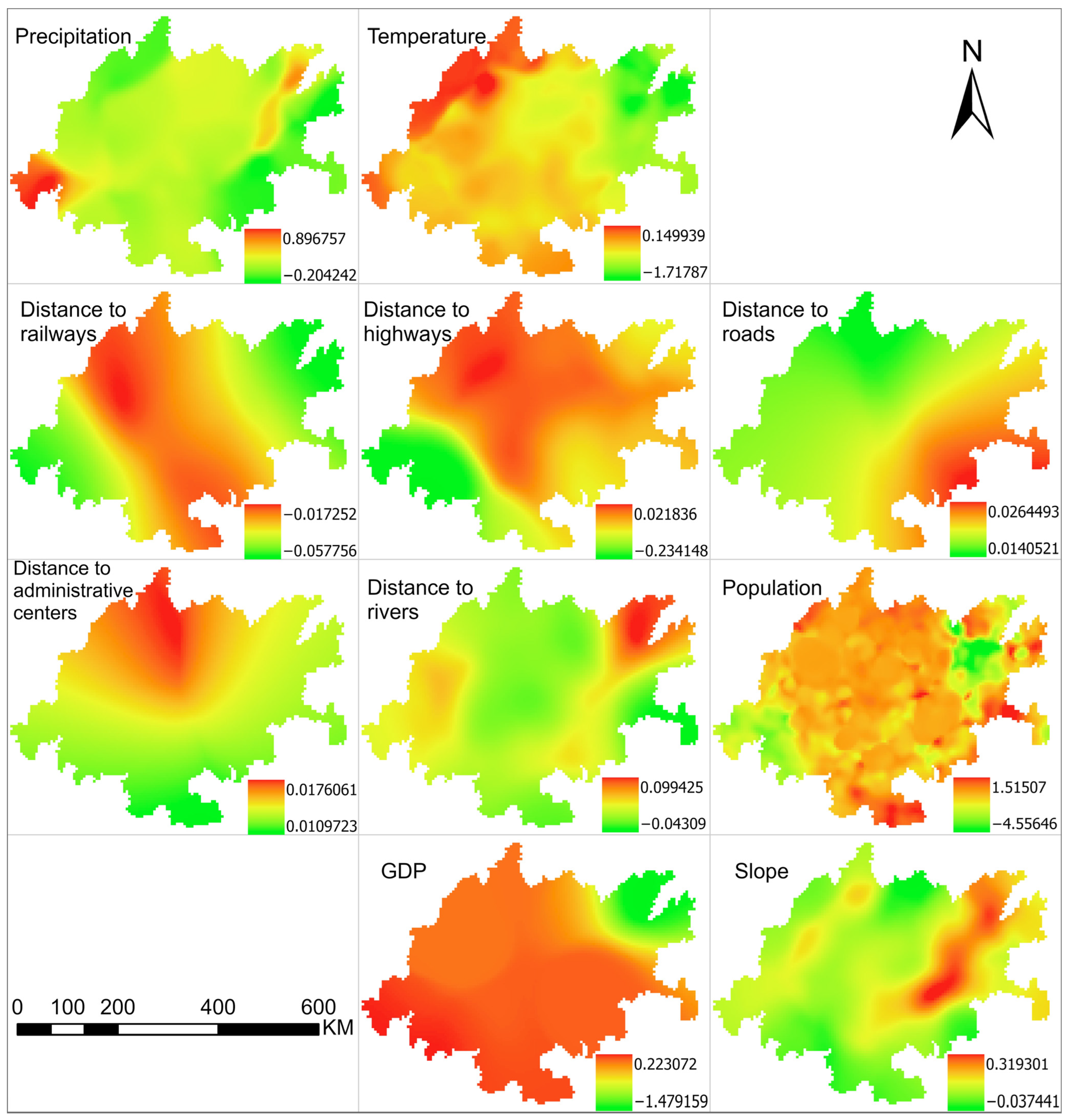
The correlation between carbon storage and various driving factors in the Chengdu–Chongqing region exhibits significant spatial heterogeneity (Figure 8), primarily due to the diverse influences of local environmental characteristics and socioeconomic conditions. The smoothness of color transitions in the Figure reflects this heterogeneity: smoother color changes indicate larger bandwidths and weaker heterogeneity, and vice versa.
Temperature has an overall negative effect on carbon storage [54], but its impact intensity varies spatially. In the western high-altitude mountainous areas, low temperatures favor the formation of forests and grasslands with strong carbon sequestration capabilities, resulting in a relatively weak inhibitory effect of temperature on carbon storage. In contrast, in urban core areas such as Chengdu and Chongqing, the combined effect of high temperatures and the rapid expansion of construction land significantly enhances the negative impact of temperature. Precipitation shows a strong positive correlation with carbon storage [54,55], though its influence varies with topographical features. In the precipitation-rich Sichuan Basin, abundant moisture significantly promotes vegetation growth, leading to higher regression coefficients in this area. In contrast, the eastern low hilly areas experience a weakened positive effect of precipitation due to limited moisture conditions.
Distance to roads is positively correlated with carbon storage, indicating that areas closer to roads face greater risks of carbon loss due to frequent human activities. Notably, the impact of roads on carbon storage in Chongqing is significantly higher than in other regions, which is related to Chongqing’s complex terrain and unique three-dimensional road network. Distance to highways, except in areas near Longquan Mountain and its southern extension, the Rongwei Dome low mountains, shows a negative correlation. These mountains are all located within the Sichuan Basin, and local topographical features may mitigate the general impact of highways. Distance to administrative centers is entirely positively correlated with carbon storage, indicating that areas farther from administrative centers have higher carbon storage levels. This phenomenon aligns with the fact that administrative centers are typically located in areas with high concentrations of construction land.
The negative impact of population density on carbon storage varies significantly due to the spatial heterogeneity of population distribution. Overall, densely populated areas exhibit a relatively weak negative effect, while in high-altitude regions, the inhibitory effect of population density on carbon storage is most pronounced.
The positive promoting effect of slope on carbon storage is widespread [13,53], with only slight negative correlations detected in 120 marginal patches. In steep mountainous areas, reduced human interference allows forest ecosystems to fully exert their carbon sink functions, making the positive effect of slope more prominent. In flat agricultural areas, frequent agricultural activities weaken the role of slope [53].
Among the non-significant variables, GDP shows a negative correlation in the northern part of the study area and a positive correlation in the southern part, with an overall unclear impact. Distance to railways is negatively correlated across the entire region, with stronger negative correlations in areas where railways are sparser. Distance to rivers and their correlation with carbon storage primarily depends on the distance between patches and rivers. This suggests that railways and rivers have no substantial impact on carbon storage.

4.2. The Critical Role of Spatial Corrections to Heterogeneity

To clarify the importance of spatial correction in heterogeneity analysis, we conducted MGWR using uncorrected carbon storage data with identical parameters and compared the results. The corrected model yielded a total Effective Number of Parameters (ENP) of 513.5, an R2 of 0.889, and a Degree of Spatial Dependency (DoD) of 0.569. In contrast, the uncorrected model produced values of 669.1 for ENP, 0.898 for R2, and 0.539 for DoD.
ENP represents the number of parameters used to fit each variable. The uncorrected MGWR model exhibited a 30.3% increase in ENP, indicating significantly higher model complexity. However, its goodness-of-fit (R2) improved by only 0.009, while DoD decreased by 0.03. This unequivocally demonstrates that the uncorrected model is overfitted—a conclusion further supported by parameter comparisons in Table 7.
Notably, the uncorrected model suggested a significantly positive impact of GDP on carbon storage, whereas the corrected model revealed the opposite relationship. This reversal aligns with empirical reality: high-GDP areas are predominantly urban built-up zones, which have a very low mean carbon storage of 0.3 t/ha. This confirms the uncorrected model obtained the wrong results.
Furthermore, administrative center data included only municipal and district-level centers, resulting in sparse and scattered sample points. Consequently, the distance to administrative centers exhibited pronounced spatial heterogeneity. Since administrative centers cluster in built-up areas, regions farther from these centers typically contain farmlands, forests, and grasslands with higher carbon storage. Thus, this factor should exert a global-scale influence rather than a neighborhood-scale effect.
These findings confirm that the uncorrected model fails to reflect valid regression coefficients and bandwidths due to overfitting. In contrast, the corrected model achieves an R2 of 0.889 without exhibiting discernible signs of overfitting.
Moreover, the spatial scale and significance of the factors identified by the two models are not entirely consistent. The correct model found that GDP, distance to roads, and distance to rivers were all insignificant (Table 6); the overfitted model suggested only GDP was insignificant. The uncorrected model reduced the effect scale of precipitation by one level (b→a), underestimated the heterogeneity of distance to railways, and significantly overestimated the heterogeneity of distance to roads, GDP, and distance to administrative centers. It proved highly unreliable.

4.3. Policy Recommendations

Several cities in the Chengdu–Chongqing region, particularly Chengdu and Chongqing, which are characterized by a high level of urbanization, have implemented policies aimed at preventing disorderly urban expansion. Notable measures include planning multiple development axes and constructing green belts to limit urban sprawl. However, under non-CP scenarios, urban sprawl remains predominantly “pancake-like” rather than following a development-along-axis pattern, indicating that current policies to restrict construction land expansion will not yield the anticipated outcomes.
Under non-ES scenarios, the Chengdu–Chongqing region experiences significant carbon storage depletion. However, the substantial reduction in cultivated land area under the ES scenario would be unacceptable. Therefore, the study area must adopt alternative measures to enhance carbon sequestration capacity within existing ecological land without large-scale expansion of ecological areas.
Cities should strictly regulate the approval process and approval rates for construction land, thus restricting the conversion of agricultural land to construction land as in the CP scenario, thereby protecting high-yield farmland near urban areas. Simultaneously, inefficient croplands in peripheral areas should be systematically guided toward transformation into forests and grasslands with high carbon storage capacity, and ultimately establish a scenario intermediate between CP and ES. Additionally, policies should be implemented to encourage construction land development along the Chengdu–Chongqing Development Axis and in remote rural areas (as projected in the BAU scenario by 2050), thus achieving a balance between cultivated land preservation, economic growth, and equitable development opportunities.
The impacts of population density and precipitation on carbon storage exhibit pronounced spatial heterogeneity. In high-density urban clusters like the Chengdu–Chongqing dual-core region, strict limits should be imposed on new construction land expansion, mandating green space ratios within built-up areas and implementing vertical greening projects to offset carbon storage loss. Moderate development may be permitted in low-density zones and along designated development corridors. Drawing from China’s ‘cultivated land balance’ policy, the study area could pilot a ‘carbon storage offset’ mechanism—requiring developers to restore equivalent areas of unused land into forests for every new construction project. Alternatively, a carbon tax equivalent to the value of destroyed carbon storage may be levied. Precipitation’s enhancement effect on carbon storage is significantly stronger in high-rainfall zones than in arid regions. Consequently, ecological restoration initiatives in high-precipitation areas will maximize carbon sequestration benefits, optimizing the climate mitigation potential of ecological lands.

4.4. Limitations

In the modeling process of PLUS, if a land use type reaches the predefined target number within a relatively short period, it becomes locked, preventing further transitions in or out. This restriction limits interactions between land use types, leading to a significantly smaller number of patches undergoing change than in reality. As a result, a land use type may predominantly transform from a single other type. This reduces the accuracy of the model and overestimates the likelihood that one land class will be converted to another, resulting in 95.4% of the new built-up land in the CP scenario being converted from forested land. Hence, carbon storage in this scenario is underestimated. In addition, when a land use type increases substantially, it is hard to reach the predetermined amounts. To illustrate, the number of construction land patches in the Chengdu–Chongqing region increased from 52,294 to 77,966 between 2010 and 2020, representing a significant expansion of 49%. When the land use pattern of 2010 was input into the model to simulate the 2020 pattern for validation, the simulation yielded 73,190 construction land patches, achieving only 81.4% of the expected conversion. In multi-scenario simulations, the process had to be divided into two stages to ensure that land use patches reached the predetermined amounts.
Despite its limitations, the PLUS model has good applicability. On the one hand, major land changes and their spatial locations are appropriately predicted. On the other hand, for smaller areas, the PLUS model usually does not need to be divided into two steps. Currently, many scholars have reported that the model has higher accuracy than other models [32,100]. Consequently, the accuracy of the model is slightly lower than but comparable to previous studies [10,101,102].

5. Conclusions

This study advances the understanding of carbon storage dynamics in rapidly urbanizing regions by integrating the PLUS model for land use simulation with the InVEST model for carbon storage assessment, complemented by MGWR to unravel spatial heterogeneity. The findings uncover the total carbon storage, its spatiotemporal dynamics, economic value, the substantial impact of urban expansion on carbon storage, and the spatial heterogeneity across the study area. This research provides critical insights for environmental analysis and management, urban planning, and development policymaking.
Urban expansion in the Chengdu–Chongqing region continues to exhibit pronounced momentum that requires stringent containment. While ecological land restoration policies should remain in effect, their implementation must be strategically refined rather than expanded indiscriminately. Future efforts should prioritize enhancing land-use efficiency within this dual-policy framework. Areas that should be converted to eco-land are steep-slope cropland with low NPP, areas with high precipitation, and unused land. New construction land should concentrate along the Chengdu–Chongqing axis, with limited allowance in existing built-up clusters, remote villages, and essential development nodes.
The ecosystem service value lost through conversion of cropland, forest, and grassland to construction land is profound—exceeding CNY 13,000 per hectare in SCC alone. Between 2015 and 2020, the study area suffered an EVCS decline of CNY 1.86 billion, representing significant socio-ecological economic damage. This loss necessitates compensation through ecological restoration programs or carbon taxation to offset negative economic externalities.
Homogenized outputs from an uncorrected InVEST model are unsuitable for spatial heterogeneity analysis. They only reveal aggregate quantities and coarse spatial patterns. In contrast, the spatially corrected MGWR results provide reliable identification of carbon storage heterogeneity, offering a robust methodological reference for future research.

Author Contributions

Conceptualization, Y.W. and K.X.; methodology, K.X. and J.Y.; software, K.X., M.L. and Y.C.; validation, K.X.; formal analysis, K.X.; investigation, K.X., M.L. and Y.C.; resources, K.X.; data curation, K.X.; writing—original draft preparation, K.X., R.L. and M.L.; writing—review and editing, K.X., R.L. and Y.W.; visualization, K.X., R.L. and J.Y.; supervision, Y.W.; project administration, K.X.; funding acquisition, Y.W. All authors have read and agreed to the published version of the manuscript.

Funding

This research was funded by Sichuan Provincial Natural Science Foundation General Program, grant number “2025ZNSFSC0256”, National Key R&D Program of China, grant number “2024YFD1700205”, National Undergraduate Training Program on Innovation and Entrepreneurship of China, grant number “202410626046”, and Research Interest Group Project of Sichuan Agricultural University, grant number “20252313”.

Data Availability Statement

The original data presented in the study are openly available at https://github.com/Wisella/Research-data-of-CS (Updated on 11 June 2025). Due to file size limitations, supplementary raw datasets are available from the first author.

Acknowledgments

We express our gratitude to the anonymous reviewers and editors for their professional comments and suggestions. We are grateful to Zhaoxu Liu for sharing the plotting code on MATLAB Central and to Yuhan Chen for her assistance in drawing Figure 6.

Conflicts of Interest

The authors declare no conflicts of interest.

Abbreviations

The following abbreviations are used in this manuscript:
SCCSocial cost of carbon
EVCSEconomic value of carbon storage
LUCCLand Use and Land Cover Change
IGBPInternational Geosphere-Biosphere Program
IHDPInternational Human Dimensions Program on Global Environmental Change
RFRandom Forest
MGWRMultiscale geographically weighted regression
LEASLand Expansion Analysis Strategy
CACellular automata
CARSMultiple Random Seeds
AICcAkaike Information Criterion with correction
BAUBusiness as usual
CPCropland protection
ESEcological security
OAOverall accuracy
GWRGeographically weighted regression
OLSOrdinary least squares
CRContribution rate of urban to carbon loss
ENPEffective Number of Parameters
DoDDegree of Spatial Dependency

References

  1. Xu, W.; Song, J.; Long, Y.; Mao, R.; Tang, B.; Li, B. Analysis and simulation of the driving mechanism and ecological effects of land cover change in the Weihe River basin, China. J. Environ. Manag. 2023, 344, 118320. [Google Scholar] [CrossRef]
  2. Li, K.; Wang, X.; Zhao, F.; An, B.; Li, P. Land use modeling and carbon storage projections of the Bosten Lake Basin in China from 1990 to 2050 across multiple scenarios. Nature 2024, 14, 27136. [Google Scholar] [CrossRef]
  3. Xu, L.; Li, Y.; Ye, W.; Zhang, X. Terrestrial organic carbon storage modes based on relationship between soil and lake carbon, China. J. Environ. Manag. 2019, 250, 109483. [Google Scholar] [CrossRef]
  4. Piao, S.; He, Y.; Wang, X.; Chen, F. Estimation of China’s terrestrial ecosystem carbon sink: Methods, progress and prospects. Sci. China Earth Sci. 2022, 65, 641–651. [Google Scholar] [CrossRef]
  5. United Nations. Millennium Ecosystem Assessment: Ecosystems and Human Well-Being: Synthesis; Island Press: Washington, DC, USA, 2005. [Google Scholar]
  6. Wang, R.Y.; Cai, H.A.; Chen, L.K.; Li, T.H. Spatiotemporal evolution and multi-scenario prediction of carbon storage in the GBA based on PLUS-InVEST models. Sustainability 2023, 15, 8421. [Google Scholar] [CrossRef]
  7. Chu, X.; Zhan, J.Y.; Li, Z.H.; Zhang, F.; Qi, W. Assessment on forest carbon sequestration in the three-north Shelterbelt Program region, China. J. Clean. Prod. 2019, 215, 382–389. [Google Scholar] [CrossRef]
  8. Lahiji, R.N.; Dinan, N.M.; Liaghati, H.; Ghaffarzadeh, H.; Vafaeinejad, A. Scenario-based estimation of catchment carbon storage: Linking multi-objective land allocation with InVEST model in a mixed agriculture-forest landscape. Front. Earth Sci. 2020, 14, 637–646. [Google Scholar] [CrossRef]
  9. Jiang, W.; Deng, Y.; Tang, Z.; Lei, X.; Chen, Z. Modelling the potential impacts of urban ecosystem changes on carbon storage under different scenarios by linking the CLUE-S and the InVEST models. Ecol. Model. 2017, 345, 30–40. [Google Scholar] [CrossRef]
  10. Wu, Q.; Wang, L.; Wang, T.; Ruan, Z.; Du, P. Spatial-temporal evolution analysis of multi-scenario land use and carbon storage based on PLUS-InVEST model: A case study in Dalian, China. Ecol. Indic. 2024, 166, 112448. [Google Scholar] [CrossRef]
  11. Kalnay, E.; Cai, M. Impact of urbanization and land-use change on climate. Nature 2003, 423, 528. [Google Scholar] [CrossRef] [PubMed]
  12. Foley, J.A.; DeFries, R.; Asner, G.P.; Barford, C.; Bonan, G.; Carpenter, S.R.; Chapin, F.S.; Coe, M.T.; Daily, G.C.; Gibbs, H.K.; et al. Global consequences of land use. Science 2005, 309, 570–574. [Google Scholar] [CrossRef]
  13. Nie, Q.; Wu, G.; Li, L.; Man, W.; Ma, J.; Bao, Z.; Luo, L.; Li, H. Exploring scaling differences and spatial heterogeneity in drivers of carbon storage changes: A comprehensive geographic analysis framework. Ecol. Indic. 2024, 165, 112193. [Google Scholar] [CrossRef]
  14. Lai, L.; Huang, X.; Yang, H.; Chuai, X.; Zhang, M.; Zhong, T.; Chen, Z.; Chen, Y.; Wang, X.; Thompson, J.R.; et al. Carbon emissions from land-use change and management in China between 1990 and 2010. Sci. Adv. 2016, 2, e1601063. [Google Scholar] [CrossRef]
  15. Nie, X.; Lu, B.; Chen, Z.; Yang, Y.; Chen, S.; Chen, Z.; Wang, H. Increase or decrease? Integrating the CLUMondo and InVEST models to assess the impact of the implementation of the Major Function Oriented Zone planning on carbon storage. Ecol. Indic. 2020, 118, 106708. [Google Scholar] [CrossRef]
  16. Hu, Y.; Batunacun; Zhen, L.; Zhuang, D. Assessment of land-use and land-cover change in Guangxi, China. Nature 2019, 9, 2189. [Google Scholar] [CrossRef]
  17. Ling, M.; Feng, Z.; Chen, Z.; Lan, Y.; Li, X.; You, H.; Han, X.; Chen, J. Evaluation of driving effects of carbon storage change in the source of the Yellow River: A perspective with CMIP6 future development scenarios. Ecol. Inform. 2024, 83, 102790. [Google Scholar] [CrossRef]
  18. Zhou, Y.; Li, Z.; Chen, Y.; Wei, W. Evaluating the corresponding relationship between the characteristics of resource utilization and the level of urbanization: A case study in Chengdu-Chongqing Economic Circle, China. Environ. Sci. Pollut. Res. 2022, 29, 55816–55829. [Google Scholar] [CrossRef]
  19. National Development and Reform Commission; Ministry of Construction. Methods and Parameters for Economic Evaluation of Construction Projects, 3rd ed.; China Planning Press: Beijing, China, 2006.
  20. Sang, L.; Zhang, C.; Yang, J.; Zhu, D.; Yun, W. Simulation of land use spatial pattern of towns and villages based on CA-Markov model. Math. Comput. Model. 2011, 54, 938–943. [Google Scholar] [CrossRef]
  21. Koomen, E.; Stillwell, J.; Bakema, A.; Scholten, H.J. (Eds.) Modelling land-use change. In The GeoJournal Library; Springer: Dordrecht, The Netherlands, 2007; Volume 90, pp. 1–22. [Google Scholar] [CrossRef]
  22. Gollnow, F.; Göpel, J.; Hissa, L.D.V.; Schaldach, R.; Lakes, T. Scenarios of land-use change in a deforestation corridor in the Brazilian Amazon: Combining two scales of analysis. Reg. Environ. Change 2018, 18, 143–159. [Google Scholar] [CrossRef]
  23. Baker, W.L. A review of models of landscape change. Landsc. Ecol. 1989, 2, 111–133. [Google Scholar] [CrossRef]
  24. Yang, Y.; Lu, Z.; Yang, M.; Yan, Y.; Wei, Y. Impact of land use changes on uncertainty in ecosystem services under different future scenarios: A case study of Zhang-Cheng area, China. J. Clean. Prod. 2024, 434, 139881. [Google Scholar] [CrossRef]
  25. Guan, D.; Zhao, Z.; Tan, J. Dynamic simulation of land use change based on logistic-CA-Markov and WLC-CA-Markov models: A case study in three gorges reservoir area of Chongqing, China. Environ. Sci. Pollut. Res. 2019, 26, 20669–20688. [Google Scholar] [CrossRef]
  26. Yang, X.; Chen, R.; Zheng, X.Q. Simulating land use change by integrating ANN-CA model and landscape pattern indices. Geomat. Nat. Hazards Risk 2015, 7, 918–932. [Google Scholar] [CrossRef]
  27. Verburg, P.H.; Soepboer, W.; Veldkamp, A.; Limpiada, R.; Espaldon, V.; Mastura, S.S.A. Modeling the spatial dynamics of regional land use: The CLUE-S model. Environ. Manag. 2002, 30, 391–405. [Google Scholar] [CrossRef] [PubMed]
  28. Verburg, P.H.; Kok, K.; Pontius, R.G.; Veldkamp, A. Modeling land-use and land-cover change. In Land-Use and Land-Cover Change: Local Processes and Global Impacts; Lambin, E.F., Geist, H., Eds.; Springer: Berlin/Heidelberg, Germany, 2006; pp. 117–135. [Google Scholar] [CrossRef]
  29. Verburg, P.H.; Overmars, K.P. Combining top-down and bottom-up dynamics in land use modeling: Exploring the future of abandoned farmlands in Europe with the Dyna-CLUE model. Landsc. Ecol. 2009, 24, 1167–1181. [Google Scholar] [CrossRef]
  30. Van Asselen, S.; Verburg, P.H. Land cover change or land-use intensification: Simulating land system change with a global-scale land change model. Glob. Change Biol. 2013, 19, 3648–3667. [Google Scholar] [CrossRef] [PubMed]
  31. Liu, X.; Liang, X.; Li, X.; Xu, X.; Ou, J.; Chen, Y.; Li, S.; Wang, S.; Pei, F. A future land use simulation model (FLUS) for simulating multiple land use scenarios by coupling human and natural effects. Landsc. Urban Plan. 2017, 168, 94–116. [Google Scholar] [CrossRef]
  32. Liang, X.; Guan, Q.; Clarke, K.C.; Liu, S.; Wang, B.; Yao, Y. Understanding the drivers of sustainable land expansion using a patch-generating land use simulation (PLUS) model: A case study in Wuhan, China. Comput. Environ. Urban Syst. 2021, 85, 101569. [Google Scholar] [CrossRef]
  33. Li, C.; Wu, Y.; Gao, B.; Zheng, K.; Wu, Y.; Li, C. Multi-scenario simulation of ecosystem service value for optimization of land use in the Sichuan-Yunnan ecological barrier, China. Ecol. Indic. 2021, 132, 108328. [Google Scholar] [CrossRef]
  34. Zhai, H.; Lv, C.; Liu, W.; Yang, C.; Fan, D.; Wang, Z.; Guan, Q. Understanding spatio-temporal patterns of land use/land cover change under urbanization in Wuhan, China, 2000–2019. Remote Sens. 2021, 13, 3331. [Google Scholar] [CrossRef]
  35. Barau, A.; Maconachie, R.; Ludin, A.; Abdulhamid, A. Urban morphology dynamics and environmental change in Kano, Nigeria. Land Use Policy 2015, 42, 307–317. [Google Scholar] [CrossRef]
  36. Cairns, G.; Goodwin, P.; Wright, G. A decision-analysis-based framework for analysing stakeholder behaviour in scenario planning. Eur. J. Oper. Res. 2016, 249, 1050–1062. [Google Scholar] [CrossRef]
  37. Dorning, M.A.; Koch, J.; Shoemaker, D.A.; Meentemeyer, R.K. Simulating urbanization scenarios reveals tradeoffs between conservation planning strategies. Landsc. Urban Plan. 2015, 136, 28–39. [Google Scholar] [CrossRef]
  38. Wu, J. Urban sustainability: An inevitable goal of landscape research. Landsc. Ecol. 2010, 25, 1–4. [Google Scholar] [CrossRef]
  39. Li, C.; Li, J.; Wu, J. Quantifying the speed, growth modes, and landscape pattern changes of urbanization: A hierarchical patch dynamics approach. Landsc. Ecol. 2013, 28, 1875–1888. [Google Scholar] [CrossRef]
  40. Li, J.; Li, C.; Zhu, F.; Song, C.; Wu, J. Spatiotemporal pattern of urbanization in Shanghai, China between 1989 and 2005. Landsc. Ecol. 2013, 28, 1545–1565. [Google Scholar] [CrossRef]
  41. Hang, J.; Sandberg, M.; Li, Y. Effect of urban morphology on wind condition in idealized city models. Atmos. Environ. 2009, 43, 869–878. [Google Scholar] [CrossRef]
  42. Luo, X.; Le, F.; Zhang, Y.; Zhang, H.; Zhai, J.; Luo, Y. Multi-scenario analysis and optimization strategy of ecological security pattern in the Weihe river basin. J. Environ. Manag. 2024, 66, 121813. [Google Scholar] [CrossRef]
  43. Chen, L.; Yao, Y.; Xiang, K.; Dai, X.; Li, W.; Dai, H.; Lu, K.; Li, W.; Lu, H.; Zhang, Y.; et al. Spatial-temporal pattern of ecosystem services and sustainable development in representative mountainous cities: A case study of Chengdu-Chongqing Urban Agglomeration. J. Environ. Manag. 2024, 368, 122261. [Google Scholar] [CrossRef] [PubMed]
  44. Yang, Y.; Li, H.; Qian, C. Analysis of the implementation effects of ecological restoration projects based on carbon storage and eco-environmental quality: A case study of the Yellow River Delta, China. J. Environ. Manag. 2023, 340, 117929. [Google Scholar] [CrossRef] [PubMed]
  45. Ye, X.; Chuai, X. Carbon sinks/sources’ spatiotemporal evolution in China and its response to built-up land expansion. J. Environ. Manag. 2022, 321, 115863. [Google Scholar] [CrossRef]
  46. Mendoza-Ponce, A.; Corona-Núñez, R.; Kraxner, F.; Leduc, S.; Patrizio, P. Identifying effects of land use cover changes and climate change on terrestrial ecosystems and carbon stocks in Mexico. Glob. Environ. Change 2018, 53, 12–23. [Google Scholar] [CrossRef]
  47. Peng, Y.; Cheng, W.; Xu, X.; Song, H. Analysis and prediction of the spatiotemporal characteristics of land-use ecological risk and carbon storage in Wuhan metropolitan area. Ecol. Indic. 2024, 158, 111432. [Google Scholar] [CrossRef]
  48. Xiang, H.; Shen, Z.; Tan, L.; Gao, C.; Wu, G.; Wang, J. Community identification and carbon storage monitoring of Heritiera littoralis with UAV hyperspectral imaging. Ecol. Indic. 2024, 167, 112653. [Google Scholar] [CrossRef]
  49. Song, M.; Huang, Z.; Chen, C.; Li, X.; Mao, F.; Huang, L.; Zhao, Y.; Lv, L.; Yu, J.; Du, H. Multi-scale geographically weighted regression estimation of carbon storage on coniferous forests considering residual distribution using remote sensing data. Ecol. Indic. 2024, 166, 112495. [Google Scholar] [CrossRef]
  50. Qiu, W.; Guo, R.; Jia, D.; Wu, M.; Wang, Z.; Zhang, L.; Jiang, L.; Li, M.; Hu, X. Spatio-temporal dynamics of global forest-urban carbon balance and its driving patterns during 1985–2020. J. Clean. Prod. 2025, 519, 145060. [Google Scholar] [CrossRef]
  51. Yang, S.; Peng, S.; Li, X.; Wei, X.; Pan, Y.; Jiao, Y. Spatial heterogeneity and interacting intensity of drivers for trade-offs and synergies between carbon sequestration and biodiversity. Glob. Ecol. Conserv. 2024, 56, e03256. [Google Scholar] [CrossRef]
  52. Luo, D.; Zhou, Z.; Zhang, L.; Chen, Q.; Huang, D.; Feng, Q.; Wu, T.; Wu, L. Evolution and driver analysis of forest carbon stocks in karst mountainous areas of southwest China in the context of rocky desertification management. CATENA 2024, 246, 108335. [Google Scholar] [CrossRef]
  53. Ji, W.; Wang, Z.; Zhang, H.; Zhang, B.; Yang, F.; Yu, Z.; Li, H.; He, M.; Lv, H.; Feng, Z. Carbon storage change, driving mechanism, and scenario prediction in Beijing-Tianjin-Hebei region for regional carbon neutral target: From history to future. Sci. Total Environ. 2025, 993, 180028. [Google Scholar] [CrossRef]
  54. Lai, J.; Qi, S.; Chen, J.; Guo, J.; Wu, H.; Chen, Y. Exploring the spatiotemporal variation of carbon storage on Hainan Island and its driving factors: Insights from InVEST, FLUS models, and machine learning. Ecol. Indic. 2025, 172, 113236. [Google Scholar] [CrossRef]
  55. Tang, J.; Peng, W. Spatiotemporal dynamics and influencing factors of land carbon stock in Chengdu Plain using an integrated model. Sci. Rep. 2025, 15, 11248. [Google Scholar] [CrossRef]
  56. Jia, X.; Han, H.; Feng, Y.; Song, P.; He, R.; Liu, Y.; Wang, P.; Zhang, K.; Du, C. Shidong Ge, Guohang Tian, Scale-dependent and driving relationships between spatial features and carbon storage and sequestration in an urban park of Zhengzhou, China. Sci. Total Environ. 2023, 894, 164916. [Google Scholar] [CrossRef]
  57. Wei, Y.; Zhou, P.; Zhang, L.; Zhang, Y. Spatio-temporal evolution analysis of land use change and landscape ecological risks in rapidly urbanizing areas based on Multi-Situation simulation—A case study of Chengdu Plain. Ecol. Indic. 2024, 166, 112245. [Google Scholar] [CrossRef]
  58. Zhang, Y.; Zhang, L.; Wang, J.; Dong, G.; Wei, Y. Quantitative analysis of NDVI driving factors based on the geographical detector model in the Chengdu-Chongqing region, China. Ecol. Indic. 2023, 155, 110978. [Google Scholar] [CrossRef]
  59. Wei, Y.; Li, Y.; Wang, S.; Wang, J.; Zhu, Y. Research on the Spatial Expansion Characteristics and Industrial and Policy Driving Forces of Chengdu–Chongqing Urban Agglomeration Based on NPP-VIIRS Night Light Remote Sensing Data. Sustainability 2023, 15, 2188. [Google Scholar] [CrossRef]
  60. Ding, Y.X.; Peng, S.Z. Spatiotemporal trends and attribution of drought across China from 1901–2100. Sustainability 2020, 12, 477. [Google Scholar] [CrossRef]
  61. Xiao, J.; Dai, J.; Fang, X.; Li, L.; Chen, G. Simulation of ecosystem service value scene in Xuzhou city based on PLUS model. Land Sci. China 2024, 38, 125–134. [Google Scholar]
  62. Yang, Y.; Yang, M.; Zhao, B.; Lu, Z.; Sun, X.; Zhang, Z. Spatially explicit carbon emissions from land use change: Dynamics and scenario simulation in the Beijing-Tianjin-Hebei urban agglomeration. Land Use Policy 2025, 150, 107473. [Google Scholar] [CrossRef]
  63. Fischer, G.; Sun, L. Model based analysis of future land-use development in China. Agric. Ecosyst. Environ. 2001, 85, 163–176. [Google Scholar] [CrossRef]
  64. López, E.; Bocco, G.; Mendoza, M.; Duhau, E. Predicting land-cover and land-use change in the urban fringe: A case in Morelia city, Mexico. Landsc. Urban Plan. 2001, 55, 271–285. [Google Scholar] [CrossRef]
  65. Masetti, G.; Robol, L. Computing performability measures in Markov chains by means of matrix functions. J. Comput. Appl. Math. 2020, 368, 112534. [Google Scholar] [CrossRef]
  66. Guan, D.; Li, H.; Inohae, T.; Su, W.; Nagaie, T.; Hokao, K. Modeling urban land use change by the integration of cellular automaton and Markov model. Ecol. Model. 2011, 222, 3761–3772. [Google Scholar] [CrossRef]
  67. Myint, S.W.; Wang, L. Multicriteria decision approach for land use land cover change using Markov chain analysis and a cellular automata approach. Can. J. Remote Sens. 2006, 32, 390–404. [Google Scholar] [CrossRef]
  68. Jenerette, G.D.; Wu, J. Analysis and simulation of land-use change in the central Arizona–Phoenix region, USA. Landsc. Ecol. 2001, 16, 611–626. [Google Scholar] [CrossRef]
  69. Su, D.; Cao, Y.; Fang, X.; Wang, J.; Cao, Y. Regional integration, agricultural production, and their heterogeneous interaction in the classic urban agglomeration of China. J. Clean. Prod. 2024, 464, 142806. [Google Scholar] [CrossRef]
  70. Yang, Y.; Bao, W.; Liu, Y. Scenario simulation of land system change in the Beijing-Tianjin-Hebei region. Land Use Policy 2020, 96, 104677. [Google Scholar] [CrossRef]
  71. Gong, J.; Hu, Z.; Chen, W.; Liu, Y.; Wang, J. Urban expansion dynamics and modes in metropolitan Guangzhou, China. Land Use Policy 2018, 72, 100–109. [Google Scholar] [CrossRef]
  72. He, J.; Li, Z.; Zhang, X.; Wang, H.; Dong, W.; Du, E.; Chang, S.; Ou, X.; Guo, S.; Tian, Z.; et al. Towards carbon neutrality: A study on China’s long-term low-carbon transition pathways and strategies. Environ. Sci. Ecotechnology 2022, 9, 100134. [Google Scholar] [CrossRef] [PubMed]
  73. Guo, W.; Teng, Y.; Yan, Y.; Zhao, C.; Zhang, W.; Ji, X. Simulation of land use and carbon storage evolution in multi-scenario: A case study in Beijing-Tianjin-Hebei urban agglomeration, China. Sustainability 2022, 14, 13436. [Google Scholar] [CrossRef]
  74. Cohen, J. A Coefficient of Agreement for Nominal Scales. Educ. Psychol. Meas. 1960, 20, 37–46. [Google Scholar] [CrossRef]
  75. Foody, G.M. Status of land cover accuracy assessment. Remote Sens. Environ. 2002, 80, 185–201. [Google Scholar] [CrossRef]
  76. Wilkinson, G.G. Results and implications of a study of fifteen years of satellite image classification experiments. IEEE Trans. Geosci. Remote Sens. 2005, 43, 433–440. [Google Scholar] [CrossRef]
  77. Monserud, R.A.; Leemans, R. Comparing global vegetation maps with the Kappa statistic. Ecol. Model. 1992, 62, 275–293. [Google Scholar] [CrossRef]
  78. Hagen-Zanker, A.; Lajoie, G. Neutral models of landscape change as benchmarks in the assessment of model performance. Landsc. Urban Plan. 2008, 86, 284–296. [Google Scholar] [CrossRef]
  79. Wang, Z.; Zeng, J.; Chen, W. Impact of urban expansion on carbon storage under multi-scenario simulations in Wuhan, China. Environ. Sci. Pollut. Res. 2022, 29, 45507–45526. [Google Scholar] [CrossRef]
  80. van Vliet, J.; Bregt, A.K.; Hagen-Zanker, A. Revisiting Kappa to account for change in the accuracy assessment of land-use change models. Ecol. Model. 2011, 222, 1367–1375. [Google Scholar] [CrossRef]
  81. Landis, J.R.; Koch, G.G. The Measurement of Observer Agreement for Categorical Data. Biometrics 1977, 33, 159–174. [Google Scholar] [CrossRef] [PubMed]
  82. McHugh, M.L. Interrater reliability: The kappa statistic. Biochem. Medica 2012, 22, 276–282. [Google Scholar] [CrossRef]
  83. Chuai, X.; Huang, X.; Lai, L.; Wang, W.; Peng, J.; Zhao, R. Land use structure optimization based on carbon storage in several regional terrestrial ecosystems across China. Environ. Sci. Policy 2013, 25, 50–61. [Google Scholar] [CrossRef]
  84. Fu, Q.; Xu, L.; Zheng, H.; Chen, J. Spatiotemporal dynamics of carbon storage in response to urbanization: A case study in the Su-Xi-Chang Region, China. Processes 2019, 7, 836. [Google Scholar] [CrossRef]
  85. Raich, J.; Nadelhoffer, K. Belowground Carbon Allocation in Forest Ecosystems: Global Trends. Ecology 1989, 70, 1346–1354. [Google Scholar] [CrossRef]
  86. Alam, S.A.; Starr, M.; Clark, B.J.F. Tree biomass and soil organic carbon densities across the Sudanese woodland savannah: A regional carbon sequestration study. J. Arid. Environ. 2017, 89, 67–76. [Google Scholar] [CrossRef]
  87. Giardina, C.P.; Ryan, M.G. Evidence that decomposition rates of organic carbon in mineral soil do not vary with temperature. Nature 2000, 404, 858–861. [Google Scholar] [CrossRef] [PubMed]
  88. Wu, F.; Wang, Z. Assessing the impact of urban land expansion on ecosystem carbon storage: A case study of the Changzhutan metropolitan area, China. Ecol. Indic. 2023, 154, 110688. [Google Scholar] [CrossRef]
  89. Tian, L.; Ye, Q.; Zhen, Z. A new assessment model of social cost of carbon and its situation analysis in China. J. Clean. Prod. 2019, 211, 1434–1443. [Google Scholar] [CrossRef]
  90. Kim, J.; Nicholls, S. Using geographically weighted regression to explore the equity of public open space distributions. J. Leis. Res. 2016, 48, 105–133. [Google Scholar] [CrossRef]
  91. Yang, Q.; Han, B. Analysis of the yield curve of China’s treasury bonds. Huabei Financ. 2013, 9, 42–45. (In Chinese) [Google Scholar]
  92. Lloyd, C.; Shuttleworth, I. Analysing commuting using local regression techniques: Scale, sensitivity, and geographical patterning. Environ. Plan. A 2005, 37, 81–103. [Google Scholar] [CrossRef]
  93. Zhou, X.; Wang, Y.C. Dynamics of land surface temperature in response to landuse/cover change. Geogr. Res. 2011, 49, 23–36. [Google Scholar] [CrossRef]
  94. Jiang, W.; Wang, Y.; Dou, M.; Liu, S.; Shao, S.; Liu, H. Solving competitive location problems with social media data based on customers’ local sensitivities. ISPRS Int. J. Geo-Inf. 2019, 8, 202. [Google Scholar] [CrossRef]
  95. Yu, S.; Hu, X.; Sheng, Y.; Zhao, C. Similarity and geographically weighted regression considering spatial scales of features space. Spat. Stat. 2025, 67, 100897. [Google Scholar] [CrossRef]
  96. Gan, L.; Halik, U.; Shi, L.; Welp, M. Multi-scenario dynamic prediction of ecological risk assessment in an arid area of northwest China. Ecol. Indic. 2023, 154, 110727. [Google Scholar] [CrossRef]
  97. Zhao, M.M.; He, Z.B.; Du, J.; Chen, L.F.; Lin, P.F.; Fang, S. Assessing the effects of ecological engineering on carbon storage by linking the CA-Markov and InVEST models. Ecol. Indic. 2019, 98, 29–38. [Google Scholar] [CrossRef]
  98. Garrigues, S.; Allard, D.; Baret, F.; Weiss, M. Influence of landscape spatial heterogeneity on the non-linear estimation of leaf area index from moderate spatial resolution remote sensing data. Remote Sens. Environ. 2006, 105, 286–298. [Google Scholar] [CrossRef]
  99. Wang, L.; Li, Y.; Gan, Y.; Zhao, L.; Fan, L.; Qin, W.; Ding, L. Reconstructing high-resolution gridded precipitation data in the southwest China highland canyon area using an improved (MGWR) downscaling method. Sci. Total Environ. 2024, 948, 174866. [Google Scholar] [CrossRef]
  100. Luan, C.; Liu, R.; Li, Y.; Zhang, Q. Comparison of various models for multi-scenario simulation of land use/land cover to predict ecosystem service value: A case study of Harbin-Changchun Urban Agglomeration, China. J. Clean. Prod. 2024, 478, 144012. [Google Scholar] [CrossRef]
  101. Zhang, J.; Wang, J.; Chen, Y.; Huang, S.; Liang, B. Spatiotemporal variation and prediction of NPP in Beijing-Tianjin-Hebei region by coupling PLUS and CASA models. Ecol. Inform. 2024, 81, 102620. [Google Scholar] [CrossRef]
  102. Zhang, C.; Jia, Q.; Liu, Y.; Zheng, Z.; Gao, Y.; Li, K. Evaluation and multi scenario simulation of ecosystem service value in Zhengzhou Metropolitan Area based on PLUS model. Meas. Sens. 2024, 32, 101079. [Google Scholar] [CrossRef]
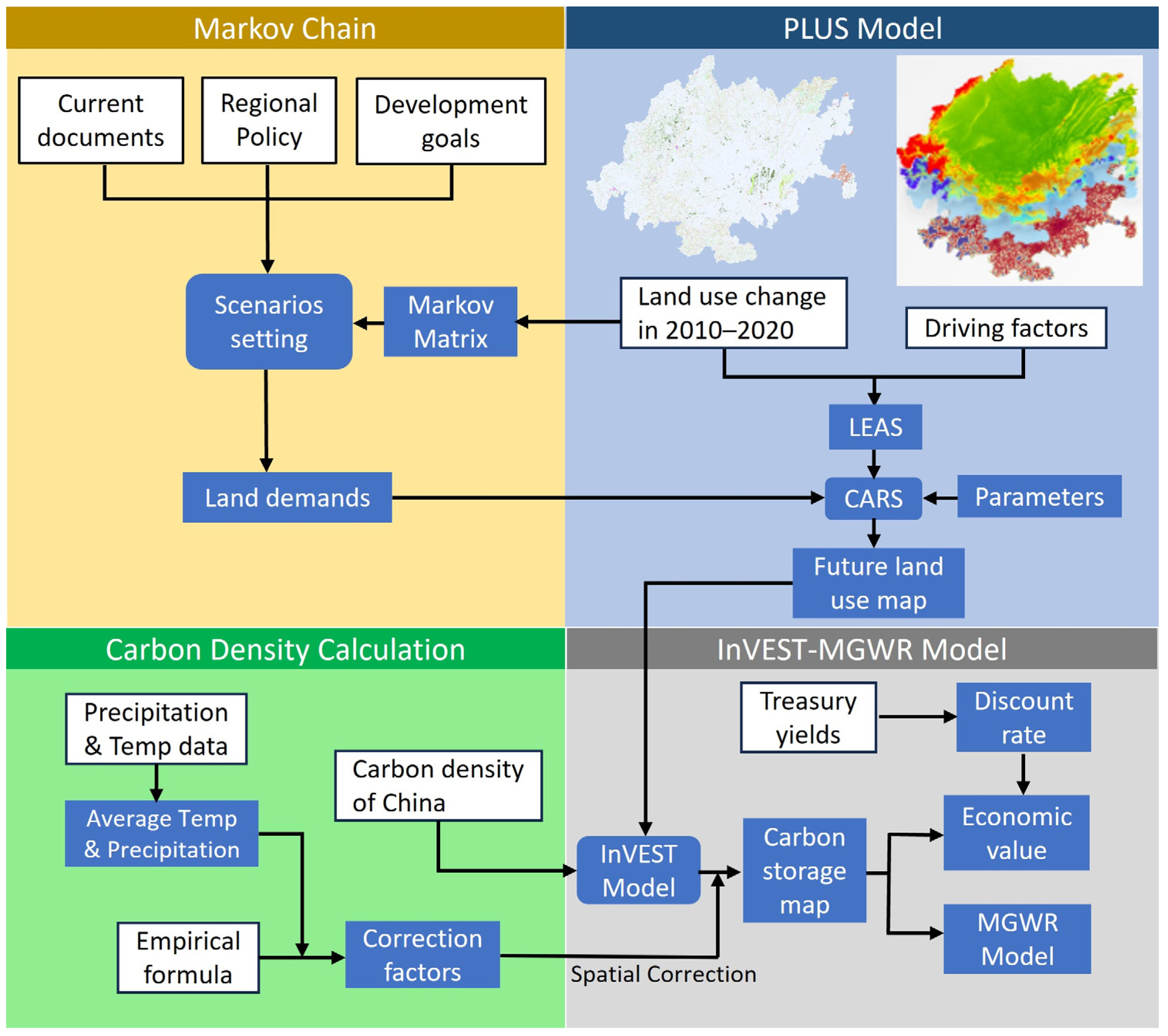
Figure 1. Overall experimental process (white-filled borders indicate externally known data.).
Land 14 01651 g001
Figure 2. Study area.
Land 14 01651 g002
Figure 3. Sankey diagrams of land use change.
Land 14 01651 g003
Figure 4. Distribution of land use in different scenarios and years.
Land 14 01651 g004
Figure 5. Carbon storage and average carbon density in various scenarios and years.
Land 14 01651 g005
Figure 6. Carbon storage in each land use type (values of scenarios are from 2050).
Land 14 01651 g006
Figure 7. Spatial change in carbon storage in the Chengdu–Chongqing region. (a) 1990–2020; (b) 2020–2030 BAU; (c) 2030 BAU–2050 BAU; (d) 2030 BAU–2050 ES; (e) 2020–2030 CP; (f) 2030 CP–2050 CP; (g) 2030 CP–2050 ES; (h) 2020–2030 ES; (i) 2030 ES–2050 ES.
Land 14 01651 g007
Figure 8. Spatial distributions of correlation coefficients.
Land 14 01651 g008
Table 1. Data sources.
TypeNameSourceTime
Basic geographic informationElevationEuropean Space Agency
(https://panda.copernicus.eu)
Accessed on 15 June 2024
2022
SlopeGenerate based on elevation2022
Annual precipitationGeographic Data Sharing Infrastructure, global resources data cloud (www.gis5g.com)
Accessed on 15 July 2024
1990–2020
Annual average temperatureNational Tibetan Plateau Science Data Center (https://data.tpdc.ac.cn)
Accessed on 13 July 2024
1990–2020
Distance to riversOpenStreetMap
(https://www.openstreetmap.org)
Accessed on 16 July 2024
2020
Socioeconomic informationPopulation densityResource and Environmental Science Data Platform (https://www.resdc.cn)
Accessed on 30 May 2024
2020
GDP density
Distance to railwaysOpenStreetMap
(https://www.openstreetmap.org)
Accessed on 16 July 2024
2020
Distance to highways
Distance to roads
Distance to administrative centersNational Bureau of Statistics
(https://www.stats.gov.cn)
Accessed on 30 May 2024
2021
Land useLUCCResource and Environmental Science Data Platform (https://www.resdc.cn)
Accessed on 15 April 2024
1990–2020
Table 2. Carbon density (t/ha).
C i _ a b o v e C i _ b e l o w C i _ s o i l C i _ d e a d
Cropland0.578.0710.842.73
Forest4.2411.5923.695.3
Grassland3.538.659.993.06
Water0.2507.80
Construction land0.3000
Unused land0.360.920.990.85
Table 3. Impact of urban expansion on carbon storage.
1990–20202020–2050
BAU
2020–2050
CP
2020–2050
ES
2020–2050
BAU-ES
2020–2050
CP-ES
Urban expansion (ha)520,380473,175172,665272,088329,508250,461
Carbon loss due to urban
expansion (106 t)
117.86109.4764.1856.9774.3478.31
Urban decrease (ha)37,95366,12362,028593123,58050,247
Carbon rise due to urban
decrease (106 t)
2.762.510.921.441.751.33
Carbon loss due to urban (106 t)115.1106.9663.2655.5372.5976.98
Total carbon change (106 t)−144.42−113.42−88.9511.71−24.49−19.66
Contribution rate of urban to carbon loss79.7%94.3%71.1%-296.4%391.6%
Table 4. Economic value of carbon storage.
Total Value
(CNY 109)
Cropland
(CNY 109)
Forest
(CNY 109)
Grassland
(CNY 109)
Water
(CNY 109)
Construction
Land
(CNY 109)
Unused Land
(CNY 109)
2015289.516153.685118.1217.230.2530.1810.046
2020287.656152.346119.03515.7390.2640.2260.045
BAU2030284.93150.275119.49514.5460.2820.2870.044
CP2030285.578153.451117.55214.0130.2730.2480.042
ES2030287.815148.764123.60714.850.290.2620.041
BAU2050280.551147.374119.60612.8370.3120.3790.043
CP2050282.098155.3114.58611.6050.2880.2820.037
ES2050288.196143.28130.67413.5590.3320.3140.037
BAU-ES285.926144.518127.36713.3430.3280.3320.038
CP-ES286.294146.687125.93313.010.320.3070.037
Table 5. Results of ordinary least squares.
VariableEstimationptVIF
Intercept00−6.509-
Temperature0.0180.5990.52615.014
Distance to administrative centers0.1430.00013.2481.436
Elevation0.1880.0005.15816.419
GDP0.0440.0412.0465.823
Distance to highways−0.710.000−6.0611.681
Population−0.1160.000−5.1666.194
Precipitation0.3140.00032.7251.140
Distance to railways0.0010.9080.1161.457
Distance to rivers−0.0080.439−0.7741.382
Distance to roads0.1000.0008.9241.544
Slope0.2740.00020.8722.127
Table 6. Results of MGWR.
VariableOLS EstMeanMedianptAdj t-val (95%)
Intercept−0.0000.082−0.0371.000−0.0002.855
Temperature−0.146−0.683−0.6480.000−10.2903.355
Distance to administrative centers0.1300.0140.0140.00012.3742.053
GDP0.050−0.1090.0300.0212.3052.430
Distance to highways−0.062−0.067−0.0480.000−5.3972.809
Population−0.121−0.445−0.1710.000−5.4173.802
Precipitation0.3130.1960.2030.00032.6073.147
Distance to railways0.005−0.034−0.0310.6190.4972.307
Distance to rivers−0.0050.0140.0080.656−0.4452.912
Distance to roads0.1010.0190.0190.0009.0252.199
Slope0.2940.1120.1040.00023.5453.159
Table 7. Degree of influence of each factor.
UncorrectedCorrected
BandwidthCoefficient RangeScaleBandwidthCoefficient RangeScale
Intercept294[−0.827, 1.012]b513[−0.773, 1.217]b
Temperature198[−1.208, 0.198]b194[−1.718, 0.150]b
Distance to administrative centers102[−0.330, 0.724]a7387[0.011, 0.018]d
GDP443[−0.293, 3.644]b1188[−1.479, 0.223]c
Distance to highways1370[−0.149, 0.015]c1129[−0.234, 0.022]c
Population47[−8.848, 4.908]a47[−4.556, 1.515]a
Precipitation102[−0.526, 2.212]a294[−0.204, 0.897]b
Distance to railways7387[−0.039, −0.034]d3575[−0.058, −0.017]d
Distance to rivers1560[−0.054, 0.038]c1239[−0.043, 0.099]c
Distance to roads2126[−0.029, 0.064]d7127[0.014, 0.026]d
Slope423[−0.110, 0.359]b443[−0.037, 0.319]b
a, b, c and d denote neighborhood scale, local scale, regional scale, and global scale, respectively.
Disclaimer/Publisher’s Note: The statements, opinions and data contained in all publications are solely those of the individual author(s) and contributor(s) and not of MDPI and/or the editor(s). MDPI and/or the editor(s) disclaim responsibility for any injury to people or property resulting from any ideas, methods, instructions or products referred to in the content.