Article

Soil Inorganic Carbon Content and Its Environmental Controls in the Weibei Loess Region: A Random Forest-Based Spatial Analysis

1
Xi’an Center of Mineral Resources Survey, China Geological Survey, Xi’an 710100, China
2
State Key Laboratory of Water Engineering Ecology and Environment in Arid Area, Xi’an University of Technology, Xi’an 710048, China
3
Development and Research Center, China Geological Survey, Beijing 100037, China
4
School of Ocean Sciences, China University of Geosciences (Beijing), Beijing 100083, China
*
Author to whom correspondence should be addressed.
Land 2025, 14(8), 1609; https://doi.org/10.3390/land14081609
Submission received: 6 June 2025 / Revised: 27 July 2025 / Accepted: 1 August 2025 / Published: 8 August 2025

Abstract

Soil carbon constitutes the largest terrestrial carbon reservoir, with inorganic forms (SIC) contributing an estimated 20–40% of the global total. Despite its relevance to arid-region carbon cycling and stabilization, SIC remains less studied than soil organic carbon (SOC). This study quantified surface SIC content (0–20 cm) and its environmental drivers across the Weibei Loess region using 3261 soil samples collected between 2008 and 2010. A combination of Random Forest (RF) modeling and optimal parameter geodetector (OPGD) analysis was employed to assess spatial heterogeneity and identify key environmental controls. SIC content ranged from 0.10 to 3.56 g kg−1 (mean = 1.23 ± 0.41 g kg−1), generally lower than reported values in the Tibetan Plateau and Inner Mongolia. Higher concentrations were observed in central areas, with lower values toward the periphery. While mean annual temperature (MAT) and precipitation (MAP) remained key climatic correlates, shortwave radiation (srad) emerged as the strongest control on SIC across the region, exhibiting a significant positive association with its accumulation. Notably, its interaction with wind speed (vs) further amplified this effect, highlighting the synergistic role of radiation and near-surface turbulence in regulating inorganic carbon retention in surface soils. Collectively, these variables explained ~56% of SIC spatial variation. Favorable conditions for SIC accumulation were identified within specific environmental thresholds: srad (171–172 W/m2), MAP (546–587 mm), MAT (10.2–11.5 °C), and vs (1.90–1.96 m/s). These findings offer a quantitative basis for understanding SIC patterns in loess-derived soils and support the development of region-specific strategies for carbon regulation under changing climatic conditions.

1. Introduction

Soils store more carbon than the atmosphere and terrestrial vegetation combined, with inorganic carbon (SIC) contributing an estimated 20–40% of the global total [1]. Despite its scale and relevance––particularly in drylands where organic matter is scarce––SIC remains significantly underrepresented in global carbon models and regional assessments [2]. In contrast to soil organic carbon (SOC), which is more vulnerable to rapid turnover and land-use disturbance, SIC represents a geochemically stable carbon pool with slower response to short-term biotic fluctuations [3]. It plays a critical role in long-term carbon stabilization, contributes to buffering capacity, and mediates key geochemical processes such as carbonate precipitation and alkalinity regulation [4]. Importantly, SIC dynamics are tightly linked to hydroclimatic conditions, and may respond strongly to projected shifts in precipitation and evapotranspiration regimes under climate change scenarios, particularly in water-limited landscapes like the Chinese Loess Plateau [5]. Yet, unlike its organic counterpart, the spatial behavior and regulatory logic of SIC remain insufficiently mapped and mechanistically understood.
The Loess Plateau in northern China provides a unique natural archive for understanding SIC formation, owing to its thick loess sediments, arid–semi-arid climate, and intensive carbonate weathering [6]. Situated on its southern margin, the Weibei Loess region lies at the interface of monsoonal and continental climates, with annual precipitation between 400–600 mm and strong evaporative demand [7]. These conditions are known to favor pedogenic carbonate accumulation. Reports indicate SIC concentrations frequently exceed 30 g/kg, with areal stocks of 100–300 Mg C/ha––substantially higher than in more humid zones [8,9]. However, the spatial pattern and regional distribution of SIC in Weibei remain poorly quantified, limiting our understanding of its carbon storage function across loess landscapes [10].
SIC formation is governed by multiple environmental factors, including climate, topography, soil chemistry, and land use [11,12]. Precipitation regulates leaching and carbonate dissolution [5], while temperature affects evaporation and mineral transformation [13]. However, in high-radiation, water-limited environments such as Weibei, the role of solar radiation and near-surface turbulence remains largely overlooked, despite their potential influence on soil moisture regimes and microclimate stability [14,15]. Vegetation cover and land use, by altering pH, organic inputs, and carbonates in the rhizosphere, also shape SIC accumulation, but are seldom integrated into multivariate analyses [16].
To address these gaps, the framework of Digital Soil Mapping (DSM) provides an effective theoretical and methodological basis for modeling soil properties across landscapes. DSM emphasizes the spatial prediction of soil attributes through statistical or machine learning models, informed by environmental covariates. A key foundation of DSM is the SCORPAN model [17], which defines soil-forming factors as a function of: Soil properties, Climatic conditions, Organisms (vegetation, fauna), Relief (topography), Parent material, Age (time), and N spatial location. Although SCORPAN has been widely applied in digital mapping of SOC, its application to SIC modeling remains rare. Integrating SCORPAN-guided covariates into machine learning approaches may thus offer a more structured and interpretable path toward understanding SIC distribution, especially under complex environmental interactions in loess systems. Moreover, in contrast to SOC, which has been extensively mapped using remote sensing and empirical models, SIC prediction remains methodologically underdeveloped, especially at fine spatial scales [18]. A more integrated understanding of both conventional and underexplored environmental controls is therefore essential to clarify the mechanisms underlying SIC variability in complex loess systems [19].
Bridging this knowledge gap requires approaches capable of quantifying spatial variation, identifying dominant controls, and capturing their interactions. In this study, we employ Random Forest (RF) modeling to estimate SIC content and identify key predictors, while using the optimal parameter geodetector (OPGD) to explore interaction mechanisms among environmental variables. Specifically, we aim to: (1) map the spatial distribution of SIC content and characterize its variability across the Weibei Loess region; (2) identify and quantify the dominant environmental controls and their interactions using a combination of RF modeling and the Geodetector method.

2. Materials and Methods

2.1. Study Area

The Weibei Loess region, located in the southern section of the Chinese Loess Plateau, spans Eastern Longitude 105°30′–110°20′ and Northern Latitude 34°10′–37°40′ [20]. The total area of the study region is approximately 1.3 × 10⁴ km2, covering diverse geomorphic and land use zones. The area lies within a typical arid–semi-arid transition zone and is characterized by a continental monsoonal climate. Average annual precipitation ranges from 400 to 600 mm, with strong interannual variability and marked seasonal concentration. Annual potential evaporation significantly exceeds precipitation, contributing to pronounced soil moisture deficits and an overall arid hydrothermal regime [21]. Geologically, the region is underlain by deep loess deposits––typically 50–150 m in thicknes––which serve as the dominant soil parent material. These deposits are rich in carbonates, providing favorable conditions for the accumulation of SIC [22]. The major soil types include Regosols (56%), Luvisols (31%), and Calcisols (11%), all developed from loess under varied topographic, climatic, and land use conditions. Land use in the region is dominated by cropland (56%), followed by grassland (26%) and forest (12%). The remaining 6% includes water bodies and urban land with limited spatial extent. Intensive anthropogenic activities such as tillage, fertilization, and vegetation disturbance have significantly altered surface soil properties, with potential implications for SIC formation and redistribution [23]. This combination of high carbonate parent material, strong climatic gradients, and mixed land use makes Weibei a representative system for investigating SIC accumulation and its environmental controls in loess-derived soils. The location of the study area is shown in Figure 1.

2.2. Soil Sampling and Laboratory Analyses

Field sampling was conducted between 2008 and 2010. A total of 3261 surface soil samples were collected from a regularly spaced sampling grid (approximately 1 sample/4 km2), designed to ensure even spatial coverage across environmental gradients. All samples were georeferenced using handheld GPS (±5 m), and sampling was confined to the 0–20 cm topsoil layer to capture the biologically active and management-sensitive zone. The sampling design, with near-uniform spatial intervals, enhances the robustness of spatial interpolation and the detection of SIC-environment relationships [24]. A spatial distribution map of all sampling points is shown in Figure 1a, and an overview of the regional environment and field sampling scenes is provided in Figure 1b.
After collection, soil samples were air-dried, manually cleaned to remove coarse debris and plant roots, and sieved to 2 mm. The homogenized samples were stored in sealed containers prior to chemical analysis. SOC concentration was analyzed using the Walkley–Black method [25], which consisted of boiling the soil-dichromate-sulfuric acid mixture for 5 min at 175 °C. Total carbon (TC) was measured through dry combustion using an elemental analyzer (2400 II CHNS/O Elemental Analyzer; Perkin–Elmer, Springfield, IL, USA). In this study, SIC concentration was calculated as the difference between TC determined by dry combustion and SOC measured using the Walkley–Black method [26].

2.3. Environmental Data

To investigate the environmental drivers of SIC content, this study compiled a comprehensive set of covariates encompassing climatic, topographic, vegetation-related, soil property, and anthropogenic factors. The selection of variables was guided by previous literature and the known controls on carbonate formation and redistribution in loess-derived soils. Climatic variables included downward shortwave radiation flux at the surface (srad), mean annual precipitation (MAP), mean annual temperature (MAT), vapor pressure deficit (vpd), and wind speed at 10 m height (vs). These variables represent key components of the regional energy and moisture balance, which are known to influence carbonate precipitation, dissolution, and atmospheric CO2 exchange. All five climatic variables were derived from the TerraClimate dataset (IDAHO_EPSCOR/TERRACLIMATE) hosted on the Google Earth Engine platform. Specifically, srad was computed as the average of monthly shortwave radiation values (W/m2) from 2008 to 2010, aligning with the soil sampling period. Similarly, MAT, vpd, and vs were obtained by averaging their respective monthly values over the same timeframe. In contrast, MAP was calculated by first averaging monthly precipitation and then multiplying by 12 to obtain the annual cumulative precipitation. Topographic features were characterized by elevation, slope, and aspect, which affect hydrological redistribution, microclimate variation, and soil formation processes. The topographic variables were directly obtained from the Geospatial Data Cloud (https://www.gscloud.cn, accessed on 4 January 2025), with the corresponding data layers labeled as “SRTMDEM”, “SRTMSLOPE”, and “SRTMASPECT”. Vegetation-related variables comprised the normalized difference vegetation index (NDVI) and vegetation type classification (vegetationtype), reflecting land surface greenness, evapotranspiration, and root-driven carbonate cycling. NDVI was derived from the Moderate Resolution Imaging Spectroradiometer (MODIS) MOD13A2 product (NASA, Washington, DC, USA), which provides 16-day composite NDVI values at 1 km resolution. NDVI values were averaged over 2008–2010 to capture vegetation greenness consistent with the soil sampling period. Vegetation type was extracted from the MODIS MCD12Q1 Land Cover Product, which offers annual land cover classifications at 500 m resolution based on the International Geosphere–Biosphere Programme (IGBP) scheme. For each pixel, the dominant vegetation type was determined as the mode of classifications from 2008 to 2010. To further represent broad-scale geomorphological patterns, a landscape classification variable was introduced to capture dominant terrain-lithology combinations across the study area. The landscape classification dataset was obtained from the Resource and Environment Science and Data Center (RESDC), Chinese Academy of Sciences (http://www.resdc.cn, accessed on 4 January 2025). Soil-related parameters included pH and soil type, both of which directly affect carbonate solubility and mineral stability. The pH values were measured concurrently during laboratory analysis of the SIC samples and were subsequently interpolated using kriging to generate continuous surface data across the study area. Soil type was derived from the Chinese 1:1,000,000 soil type spatial vector dataset compiled in 1995, considering that soil classification is relatively stable over time. To account for anthropogenic influences, nightlight intensity data from RESDC were included as a spatially continuous indicator of human activity density. The dataset was calculated as the mean of annual nightlight values from 2008 to 2010.
All environmental variables were first processed through resampling, reprojection, clipping, and geometric correction, and then standardized into raster format with a spatial resolution of 1 km to ensure consistency. Missing or invalid values were imputed using the local mean of a 5 × 5 pixel moving window. The resulting dataset provided a spatially aligned environmental variable stack for statistical modeling. A summary of data sources and variable descriptions is provided in Table 1.

2.4. Statistical Modeling and Key Covariates Selection

To model the spatial distribution of SIC content and identify its key environmental controls, a RF regression model was constructed using the ranger package in R 4.1.0 version [27]. The modeling process began by extracting environmental covariates corresponding to each of the 3261 sampling points, resulting in a data matrix linking measured SIC values with predictor variables. The full dataset was randomly partitioned into a training set (80%) and a validation set (20%) to evaluate model generalizability.
To distinguish between model construction and key covariates selection, we separated the RF modeling into two distinct stages. The initial model was trained using the full set of covariates and tuned to achieve the highest predictive accuracy, which was subsequently used for spatial SIC estimation. In contrast, key covariates selection were conducted solely for the purpose of identifying the most influential environmental drivers. This separation ensured that the SIC estimation model maintained high predictive accuracy, while the identification of key predictors remained ecologically meaningful and interpretable.
Initial model construction was performed using default settings in the “ranger” package in R 4.1.0 version [28]. Subsequently, model hyperparameters were optimized using the “tuneRanger” package (https://github.com/PhilippPro/tuneRanger, accessed on 4 January 2025), which applies a model-based optimization strategy to simultaneously tune the key parameters “mtry”, “sample.fraction”, and “min.node.size” that influence model complexity and predictive performance. This tuning was performed based on out-of-bag (OOB) error estimates, which avoid data leakage and reduce computational cost compared to conventional k-fold cross-validation. The tuning objective was to maximize the coefficient of determination (R2) and minimize the mean squared error (MSE), and the final selected configuration represented the best-performing model under these criteria. Based on the optimized predictive model, a five-fold cross-validation repeated 100 times was also conducted to calculate the average root mean square error (RMSE) and further assess the model’s robustness.
To identify the key environmental covariates driving the spatial distribution of SIC, variable importance was first assessed using the Mean Decrease in Accuracy (MDA) index derived from the RF model. However, because this importance ranking can be confounded by multicollinearity—where strongly correlated predictors exhibit inflated or indistinguishable importance values—a two-stage variable selection strategy was implemented (as shown in VIF Rounds 1–3 and VI Rounds 1–3 in Table 2).
In the first stage, covariates with variance inflation factor (VIF) values greater than 10 were flagged for removal due to potential multicollinearity. Instead of eliminating all high-VIF variables simultaneously, a stepwise reduction approach was adopted. In each iteration, one variable was excluded based on a joint consideration of (1) statistical multicollinearity metrics and (2) ecological relevance derived from expert knowledge. This process continued until all retained variables satisfied the VIF < 10 criterion, ensuring that the final model inputs were not only statistically independent but also ecologically interpretable. Additionally, special attention was given to variables with inherently composite environmental meanings. For example, elevation and vpd integrate multiple physical gradients such as temperature, radiation, and humidity, making their individual mechanistic roles more ambiguous. In contrast, variables with univariate physical significance, such as MAT, offer clearer interpretive value. Despite MAT exhibiting the highest VIF (31.585) among the three variables (compared to 24.583 for elevation and 20.944 for vpd) (VIF Round 1 in Table 2), we retained MAT and removed elevation and vpd. This decision was based on the principle of preserving variables with distinct climatic interpretability, especially when ecological relevance has been consistently demonstrated in dryland carbon studies. After removing elevation and vpd, the VIF of MAT decreased to 8.305 (VIF Round 3 in Table 2), confirming that much of its multicollinearity was attributable to those variables. The model’s predictive performance (R2 and MSE) remained stable throughout this refinement (Table 2), validating the necessity of eliminating multicollinear covariates.
In the second stage, once multicollinearity was adequately resolved, further refinement was carried out based exclusively on variable importance. Specifically, the least important variables (those with lower MDA scores) were removed iteratively (VI Rounds 1–3 in Table 2), and a new RF model was trained at each step. The resulting model performance (R2 and MSE) was compared to the best-performing model (VIF Round 1 in Table 2), and variable elimination was halted once model accuracy deviated by more than 5% from the maximum R2 and minimum MSE. The final set of retained predictors—those whose removal would significantly impair model performance—were thus identified as the key environmental drivers of SIC distribution in the study area. Finally, the significance of these key covariates was further validated using 10-fold, five-times repeated cross-validation implemented via the “rfcv” function from the “randomForest” package.
To further examine the direction and strength of these relationships, partial dependence plots (pdp) [29] were generated for key predictors. These plots allowed us to isolate the marginal effect of each variable on SIC content while controlling for the influence of other variables.

2.5. Geographical Detector Model with Optimal Parameters (OPGD)

To assess how environmental variables interact to regulate SIC spatial differentiation, we applied the Geographical Detector (GeoDetector) method [30]. The q-statistic was used to quantify the explanatory power of each factor, as well as their pairwise interactions, under conventional environmental conditions. This approach allowed for the identification of synergistic or antagonistic effects among variables beyond their individual contributions. The model comprises the following core modules:
(1) Factor Detection: This module calculates the explanatory power (q-value) of each factor for the spatial distribution of SIC. A larger q-value indicates a more significant impact of the factor on SIC. The calculation formula is as follows:
q = 1 1 N σ 2 h = 1 L N h σ h 2 = 1 S S W S S T
S S W = h = 1 L N h σ h 2
S S T = N σ 2
In the formula: h = 1, 2, …, L represents the categories of SIC and driving factors; the q-value ranges from 0 to 1, where a larger q-value indicates a stronger influence of the driving factor on the spatial differentiation of SIC; N h and N denote the total number of samples in the h-th category and the entire study area, respectively; σ h 2 and σ 2 represent the variances of SIC in the h-th category and the entire study area, respectively. S S W and S S T respectively represent the sum of variances of L categories and the total variance of the region.
(2) Interaction Detection: This module analyzes the interaction between two factors to determine whether their combined effect is enhancing, independent, or weakening. The interaction type is identified using the q-value of their intersection, denoted as [q(X1 ∩ X2)], as summarized in Table 3:
(3) Optimal Threshold Detection: In recent years, researchers have developed the Optimal Parameter Geographical Detector (OPGD) model [31], which integrates machine learning algorithms (e.g., K-means, decision trees) to optimize the classification of environmental factors affecting SIC and calculate optimal spatial scale parameters under different classification methods. This study employed the OPGD model to identify the optimal environmental conditions for SIC accumulation, aiming to further refine SIC regulation strategies. The specific calculation formula is as follows:
t = Y ¯ h = 1 Y ¯ h = 2 V a r ( Y h = 1 ) n h = 1 + V a r ( Y h = 2 ) n h = 2 1 2
In the formula, Y ¯ denotes the mean value of the linear regression coefficients for SIC within subregion h; n h is the number of samples in the subregion h; V a r represents the variance.

3. Results

3.1. Model Performance

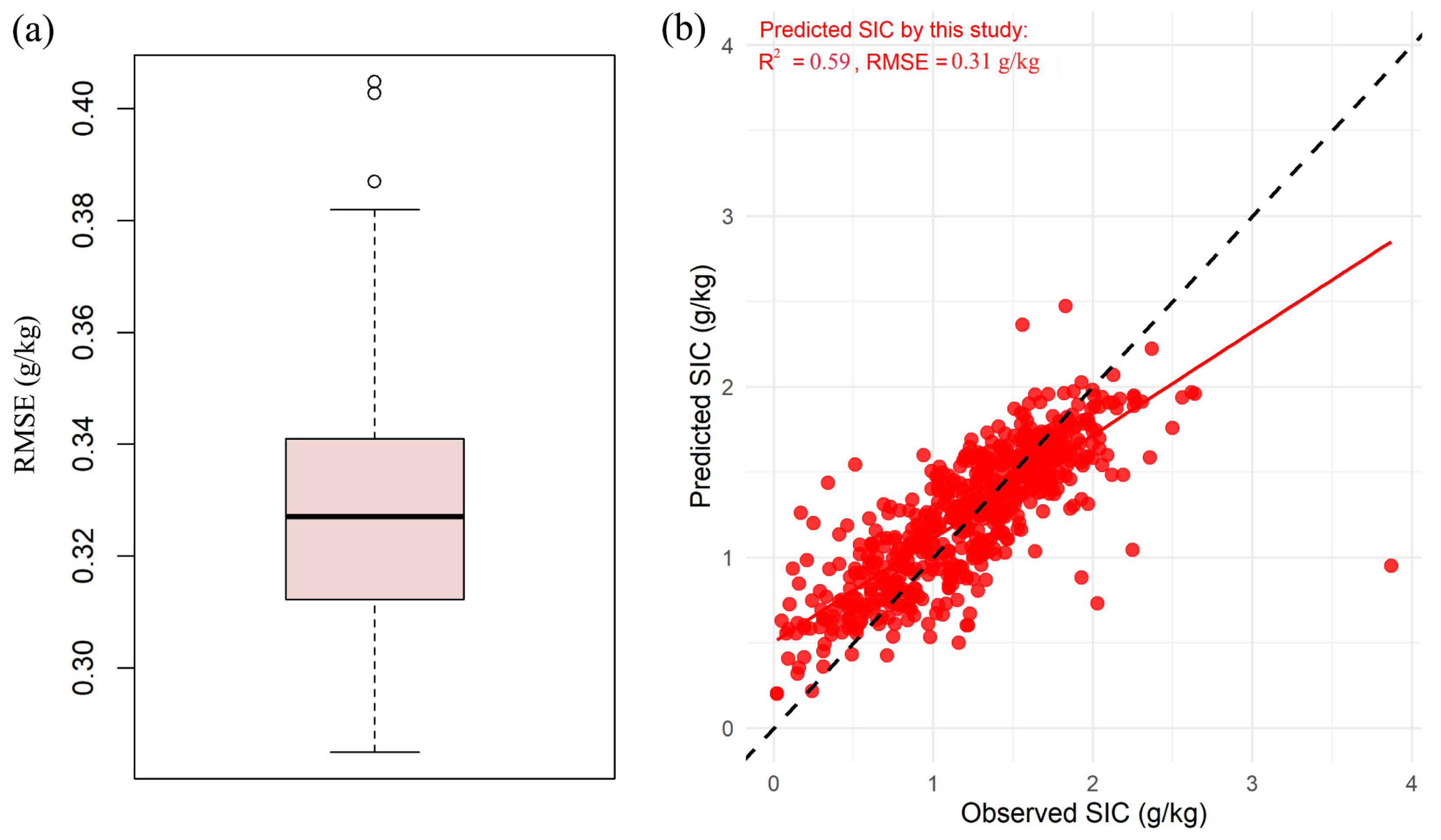
The RF model with all candidate environmental covariates, optimized using the tuneRanger function, achieved a maximum modeling accuracy with an R2 of 0.621 and a MSE of 0.1057 g2/kg2 (Table 2). When evaluated on the independent validation dataset (20% hold-out), the model yielded an R2 of 0.590 and RMSE of 0.310 g/kg (Figure 2b), indicating stable generalization performance.
To further assess the robustness of the model, a 100-repeated five-fold cross-validation was conducted. The average RMSE across all cross-validation folds was 0.328 g/kg, with most values concentrated between 0.312 and 0.341 g/kg (Figure 2a), suggesting low variability in model accuracy under different data partitions. The predicted SIC content closely matched observed values in the validation set (Figure 2b), and data points were largely aligned along the 1:1 line, confirming the model’s reliable predictive capacity and lack of systemic bias.

3.2. Spatial Variation and Distribution of SIC Content

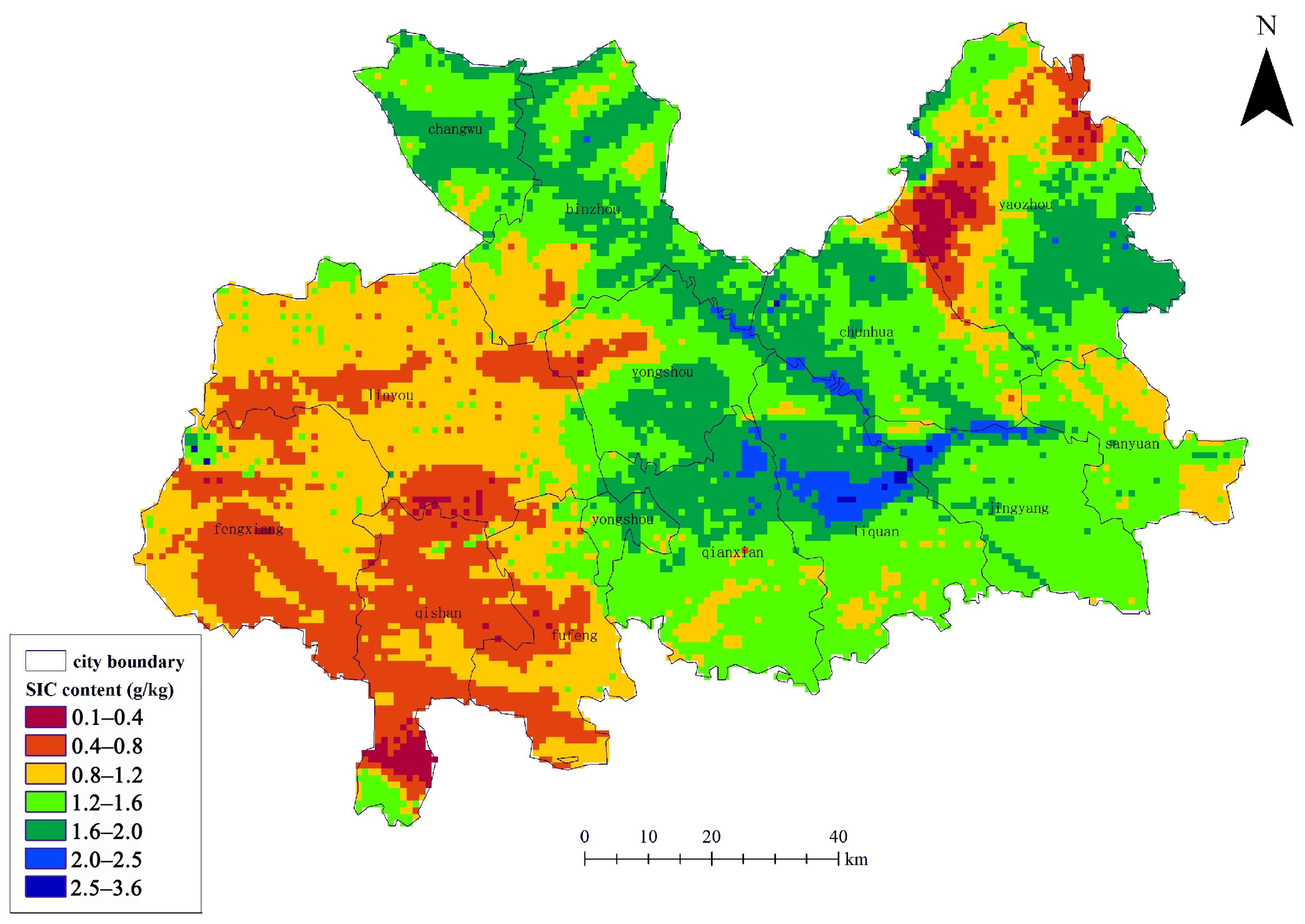
The surface SIC content across the study region ranged from 0.10 to 3.56 g/kg, with a mean value of 1.23 ± 0.41 g/kg and a coefficient of variation (CV) of 37.4% (Figure 3). Spatially, SIC content exhibited clear zonal and patchy distribution patterns. High-value stripes oriented southeast–northwest were observed in the central and eastern areas, whereas patchy low-value zones were distributed in the southwestern and northeastern parts of the region. The majority of the area was classified as medium-content (0.8–1.6 g/kg), while low-content areas (0.1–0.8 g/kg) and high-content areas (1.6–3.6 g/kg) appeared less frequently (Figure 3).
SIC content also showed substantial variation across administrative units (Table 4). The overall range at the county level spanned from 0.10 g/kg (Qishan) to 3.56 g/kg (Liquan), with an average value of approximately 1.20 g/kg. The greatest intra-county range was observed in Fengxiang (2.64 g/kg), while Changwu exhibited the narrowest range (0.95 g/kg). Mean SIC content varied notably among counties, with the lowest average found in Qishan (0.71 g/kg) and the highest in Liquan (1.58 g/kg). Standard deviation (Std) values indicated differences in intra-county variability, ranging from 0.17 g/kg in Changwu to 0.46 g/kg in Yaozhou, reflecting relatively homogeneous and heterogeneous distributions, respectively, within these locations.

3.3. The Independent Driving Effect of Key Covariates on SIC

After removing two collinear variables, elevation and vpd, the VIF values for all remaining variables were reduced to below 10 (Table 2). The model based on this reduced variable set retained stable accuracy, with an R2 of 0.603 and MSE of 0.110 g2/kg2, both within 5% of the full model’s best performance (Table 2). Subsequently, variables with the lowest importance were iteratively removed. After two rounds of reduction, six relatively unimportant variables (aspect, landscape, nightlight, slope, soil type, and vegetation type) were excluded (Table 2). The final model—constructed using the most important predictors—reached the threshold of acceptable performance deviation, with an R2 of 0.590 (4.99% lower than the maximum) and an MSE of 0.111 g2/kg2 (5.01% higher than the minimum) (Table 2), thereby defining the most parsimonious model that retained optimal predictive capacity.
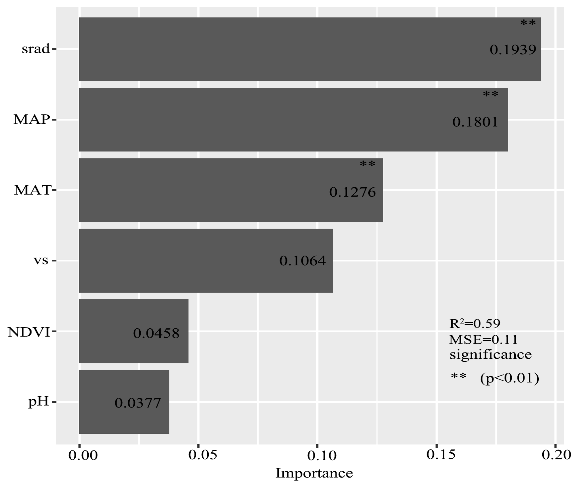
The final set of key covariates of SIC content, ranked by MDA, included solar radiation (srad, 0.193), mean annual precipitation (MAP, 0.180), mean annual temperature (MAT, 0.127), wind speed (vs, 0.106), NDVI (0.045), and soil pH (0.037) (Table 2, Figure 4). Repeated cross-validation confirmed that srad, MAP, and MAT significantly contributed to the prediction of SIC distribution, while vs, though not statistically significant, ranked among the top four most important covariates (Figure 4). Collectively, these four variables explained approximately 56% of the spatial variation in SIC.
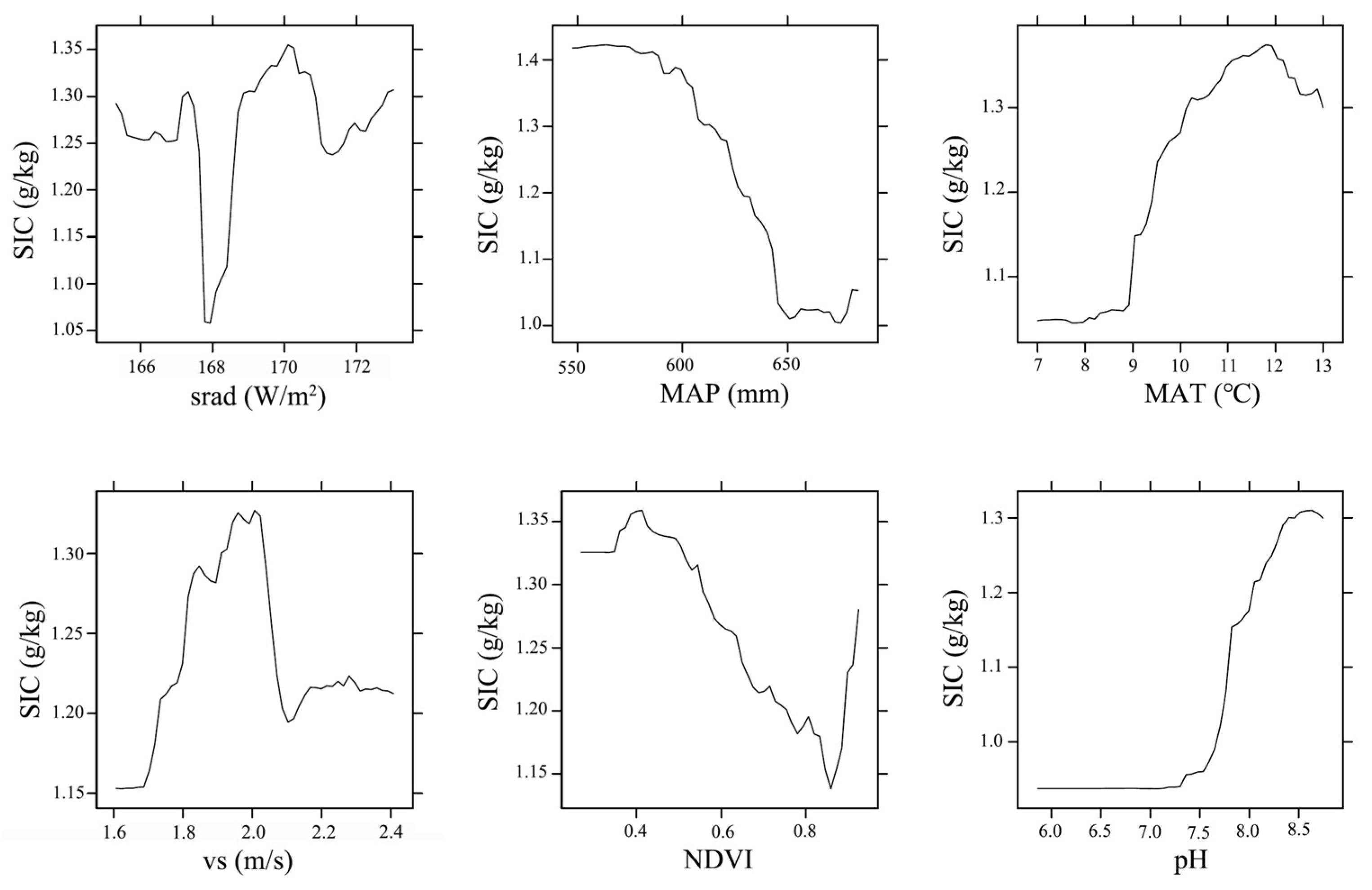
The partial dependence analysis showed distinct response curves for each covariate (Figure 5).
SIC content exhibited a complex, non-monotonic response to variations in srad. When srad was below approximately 167 W/m2, SIC content showed a general declining trend, with a steeper decrease at lower radiation levels. Between 167 and 167.5 W/m2, SIC values rose slightly, followed by a sharp decline from 167.5 to 168 W/m2, where the lowest SIC values were observed. From 168 to 170 W/m2, SIC content increased rapidly, reaching its overall peak. A subsequent sharp decline occurred between 170 and 171 W/m2, followed by a moderate increase up to around 173 W/m2. Apart from the sharp fluctuation near 168 W/m2, SIC values at other srad levels were predominantly above 1.23 g/kg; SIC content exhibited a consistent negative trend within the 550–650 mm range of MAP. Beyond 650 mm, the decline in SIC values plateaued, indicating no further reduction with increased precipitation; SIC content remained consistently low at MAT < 9 °C. A sharp increase was observed between 9 °C and 11.5 °C, after which SIC content began to decrease again. The curve exhibited a unimodal pattern with a peak near 11.5 °C; SIC content increased steadily up to approximately 20 m/s of vs. Between 20 m/s and 21 m/s, the content decreased, followed by a relatively stable trend at higher wind speeds; Partial dependence analysis revealed a nonlinear relationship between NDVI and SIC. When NDVI values were below 0.4, SIC content remained relatively high and showed a slight increasing trend. However, once NDVI exceeded 0.4, SIC content declined sharply, reaching its minimum near NDVI = 0.85. Beyond this point, SIC content began to increase again. At pH values below 7.5, SIC content remained at relatively low levels. A rapid increase was observed as pH rose above 7.5, peaking around pH 8.5. This trend indicated a clear threshold response associated with alkaline soil conditions.
Collectively, these results show that srad, MAP, and MAT were the most influential predictors of SIC content variation across the region, while srad and vs exhibited more complex, nonlinear, or threshold-dependent effects.

3.4. Nonlinear Enhancement Effect of Two-Factor Interaction

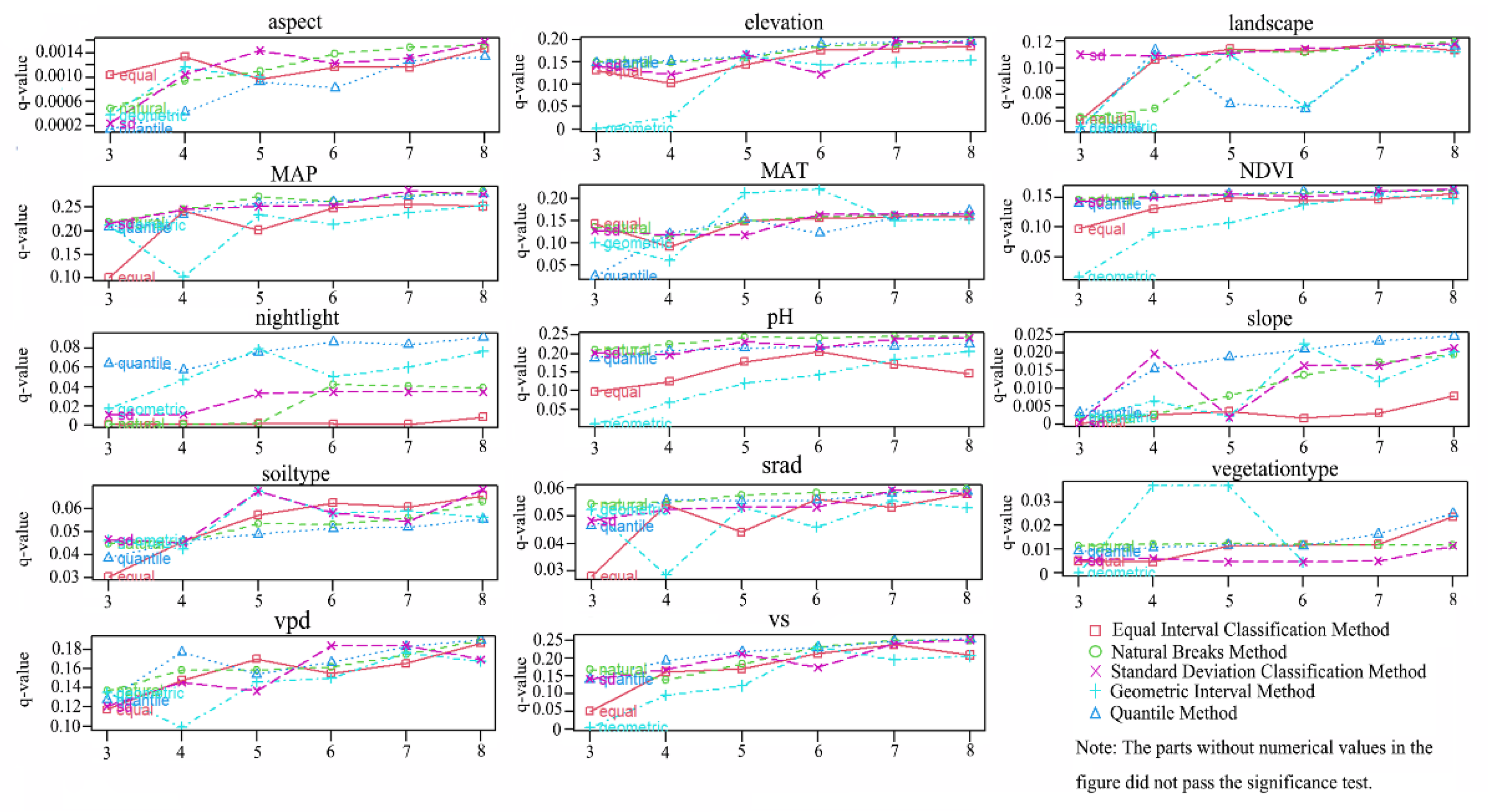
Based on the traditional factor detection method of Geographical Detector, we set the classification levels of explanatory variables to 3–8 classes using R 4.1.0 version software (https://www.r-project.org, accessed on 4 January 2025) (Figure 6). Five discretization methods were employed for optimal partitioning: Natural Breaks, Standard Deviation Breaks, Geometric Breaks, Quantile Breaks, and Equal Interval Breaks. This approach improved the accuracy and precision of the model.
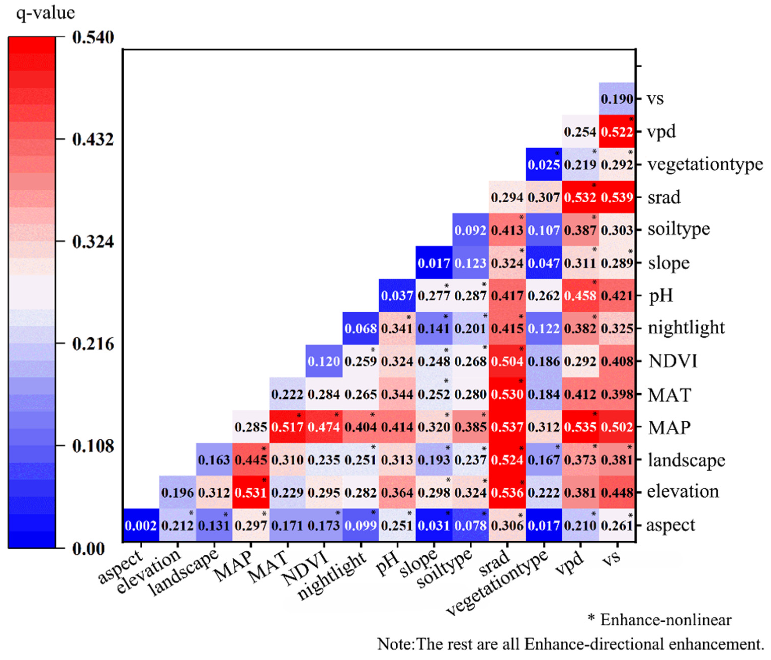
To investigate the effects of interactions between natural and anthropogenic factors on SIC content changes, we used the Optimal Parameter Geographical Detector (OPGD) model to calculate the driving forces of interactions between different drivers. Factor detection results (seen in Figure 7) showed that all pairwise driver interactions exhibited bivariate or nonlinear enhancement, with no independent interactions identified: specifically, bivariate interaction q-values exceeded those of single-factor effects. The strongest interaction driving SIC content was between srad and vs (q = 0.539), indicating their interaction is a primary cause of SIC variability and spatial differentiation in the area. The top five bivariate interaction q-values were srad∩vs (0.539) > srad ∩ MAP (0.537) > srad ∩ elevation (0.536) > vpd ∩ MAP (0.535) > vpd ∩ srad (0.532). Notably, 12 factor interactions had q-values > 0.5, strongly demonstrating that driver interactions significantly amplify spatiotemporal variations in SIC content.

3.5. Optimal Environmental Conditions Accumulated by SIC

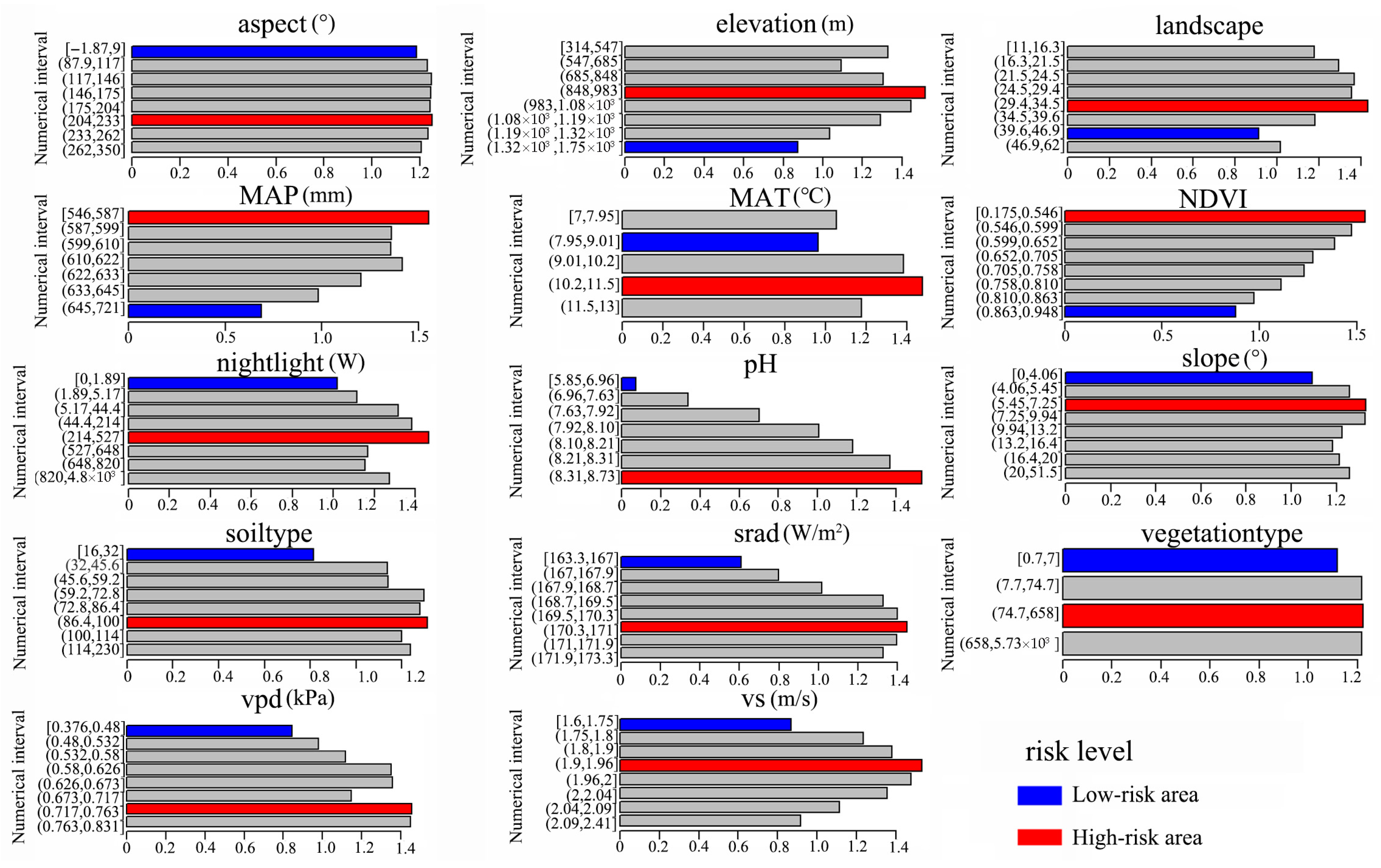
Based on risk zone detection results from the Geographical Detector (seen in Figure 8), optimal factor ranges or types conducive to SIC accumulation were identified. Specifically, these included an aspect of 204–233°, elevation of 848–983 m, forest landscape, MAP of 546–587 mm, MAT of 10.2–11.5 °C, NDVI of 0.175–0.546, nightlight of 214–527 W, pH of 8.31–8.73, slope of 5.45–7.25°, regosols soiltype, srad of 171–172 W/m2, broad-leaved forest vegetationtype, vpd of 0.717–0.763 kPa, and vs of 1.90–1.96 m/s. These driving factor ranges or types promote SIC accumulation in the study area.

4. Discussion

4.1. Regional Heterogeneity and Significance of SIC Patterns in the Weibei Loess Region

Despite increasing attention to soil inorganic carbon (SIC) in dryland systems, comprehensive, high-density analyses at fine spatial scales remain limited across the Chinese Loess Plateau [32]. This study provides the first regional-scale, grid-based assessment of surface SIC content in the Weibei Loess region using 3261 uniformly distributed samples. Compared to prior studies that relied on sparse or administrative-unit-aggregated data, our sampling framework enabled continuous SIC estimation and spatial pattern analysis at the county level, revealing pronounced heterogeneity both across and within local administrative units.
For instance, average SIC content differed markedly between Liquan (1.58 g/kg) and Qishan (0.71 g/kg), two counties located within the same climatic zone. This contrast highlights the spatial imprint of land use and human activity intensity on SIC dynamics [19,33]. Liquan, located at the transition between loess tablelands and river terraces, experiences relatively low vegetation coverage, limited tillage disturbance, and strong evaporative conditions––conditions conducive to carbonate precipitation and accumulation. In contrast, Qishan is situated in a densely cultivated alluvial plain, with high-intensity agricultural practices (e.g., fertilization, irrigation, tillage) and deeper leaching potential, resulting in significantly depleted SIC levels [34,35]. These localized disparities provide mechanistic insights into how environmental gradients and anthropogenic disturbance jointly shape SIC variability.
Relative to other dryland regions, the Weibei Loess Region exhibits substantially lower average SIC levels. Previous studies report mean SIC contents of ~2.1 g/kg in the Inner Mongolian grasslands and ~5.1 g/kg in the Tibetan Plateau [36]. These regional differences can be primarily attributed to divergent parent material characteristics, pedogenic processes, and climatic controls [37]. In the Tibetan Plateau, low atmospheric CO2 partial pressure at high altitudes promotes carbonate precipitation, while relatively young soils retain significant lithogenic inorganic carbon (LIC) [38]. The Inner Mongolian grasslands, meanwhile, exhibit abundant primary carbonates, low leaching risk, and minimal anthropogenic disturbance, all of which favor SIC preservation [39]. In contrast, soils in Weibei derive from leached loess with modest carbonate reserves, are subject to moderate hydrothermal regimes that facilitate carbonate dissolution, and experience high-intensity land use pressure that enhances SIC depletion [40].
Taken together, these comparisons emphasize the importance of both macro-scale controls (e.g., climate regime) and fine-scale processes (e.g., land use intensity, erosion risk) in determining regional SIC patterns. While the present study provides valuable insights into SIC dynamics at a regional scale, it may not fully capture broader continental or national-scale variability due to differences in soil genesis, climatic gradients, and land management practices beyond the Weibei context. Nonetheless, this work fills a critical knowledge gap by linking 1 km-resolution SIC estimates with multi-scalar environmental drivers in one of China’s most intensively managed dryland systems and offers a methodological foundation that could be adapted for larger-scale applications with further data integration.

4.2. Mechanistic Insights into Dominant and Interactive Environmental Drivers of SIC

The spatial differentiation of SIC in arid–semi-arid landscapes arises from a complex interplay of environmental factors [41]. Through RF modeling and optimal-parameter Geodetector analysis, this study identified srad, MAP, MAT, and vs as the principal drivers of SIC variation in the Weibei Loess region.
Among the key environmental controls identified in this study, srad exhibited the strongest explanatory power for SIC distribution in the Weibei Loess region. The dominant influence of srad can be attributed to its role in intensifying evaporative processes at the soil–atmosphere interface, thereby driving carbonate supersaturation and the precipitation of pedogenic inorganic carbon [42]. Under arid and semi-arid conditions, enhanced solar input accelerates soil water evaporation, which increases carbonate ion concentrations in the soil solution and facilitates the formation of calcium carbonate nodules, especially in near-surface layers where atmospheric exchange is strongest [43].
Moreover, this study revealed a complex, non-monotonic response of SIC content to increasing srad values, with multiple inflection points. Specifically, SIC content declined with increasing srad up to ~168 W/m2, reaching a pronounced minimum. This phase likely corresponds to a threshold where evaporation-induced carbonate accumulation is offset by carbonate destabilization mechanisms, such as CO2 loss through microbial respiration or enhanced leaching due to intermittent precipitation events. A sharp increase in SIC was then observed from 168 to 170 W/m2, suggesting that beyond a certain energy threshold, the evaporation rate may reach a level that favors net carbonate accumulation once again, especially under water-limited conditions with reduced leaching potential. This is consistent with findings from arid ecosystems in Central Asia and the southwestern U.S., where solar radiation intensity above critical thresholds has been linked to the formation of caliche layers and carbonate-rich horizons [44,45]. Interestingly, the interval between 170 and 171 W/m2 showed a steep decline in SIC, followed by a moderate recovery up to ~173 W/m2. These oscillations may reflect the competing effects of photodegradation, wind-induced CO2 diffusion, and carbonate dissolution feedback, which remain underexplored in existing SIC models. Recent studies suggest that high radiation exposure can stimulate photodegradation of surface organic matter, releasing CO2 that may shift the carbonate equilibrium towards dissolution under certain soil pH and moisture conditions [46]. Additionally, soil surface temperature, which strongly correlates with srad, may influence microbial activity, indirectly affecting carbonate stability. Notably, despite these fluctuations, SIC remained relatively high (above 1.23 g/kg) in most srad intervals, underscoring the overall facilitating role of solar radiation in sustaining carbonate accumulation across varied microenvironments. This aligns with regional studies in the Loess Plateau and arid zones of northern China, which have reported positive associations between solar exposure and SIC stocks, especially in uncultivated or lightly managed areas [47].
Collectively, these findings emphasize that srad is not merely a background climatic variable but acts as a mechanistic driver of SIC formation and spatial variability. Its effects are particularly pronounced in regions like the Weibei Loess Platform, where fine-textured soils, parent material richness in carbonate, and strong seasonal desiccation form a conducive setting for radiatively driven carbonate processes. Future research should aim to quantify energy balance components and incorporate radiative forcing indices into SIC models, particularly under scenarios of climate change where solar radiation regimes may shift.
The negative relationship between MAP and SIC aligns with carbonate leaching theory: increased precipitation enhances water infiltration and subsurface transport, promoting carbonate dissolution and downward loss [48]. The limited contribution of MAT is likely linked to the region’s narrow thermal gradient (ΔMAT ≈ 3.2 °C), which reduces the temperature’s spatial signal strength. This diverges from patterns observed in broader-scale studies such as those in the U.S. Great Plains, where MAT plays a more prominent role due to stronger latitudinal gradients [49].
Unlike arid regions where high NDVI values are uncommon, NDVI values in the Weibei Loess Region are concentrated within the 0.4–0.8 range, reflecting substantial vegetation coverage under croplands, grasslands, and forest restoration programs. The observed decline in SIC within this NDVI range is thus supported by robust sample representation, rather than resulting from data sparsity or model bias. A threshold-like pattern emerged: SIC content increased slightly with NDVI up to ~0.4, remained relatively stable between 0.4 and 0.6, and then declined sharply beyond 0.6. This decline likely reflects enhanced biological processes associated with denser vegetation, such as intensified root respiration, organic acid exudation, and microbial activity—all of which contribute to lower pH and accelerated carbonate dissolution [50]. These mechanisms are well-documented in semi-humid loess systems where biological acidification depletes soil carbonates. The minor SIC rebound observed at NDVI > 0.85, although based on fewer samples, may be attributed to local factors such as carbonate-enriched substrates or reduced acidity under certain forest plantations. Nonetheless, this should be interpreted with caution due to potential edge effects in the model [51]. Collectively, these findings suggest that NDVI influences SIC through nonlinear, stage-dependent pathways rather than a monotonic gradient. This underscores the need for regionally calibrated models that account for the complex interactions among vegetation structure, biological activity, and soil carbonate dynamics in loess landscapes.
Importantly, our results revealed that interaction effects between environmental variables often surpassed their individual contributions. For example, the combined effect of srad and vs exerted a particularly strong influence on SIC spatial distribution. These two variables jointly reflect synergistic hydrothermal dynamics––enhanced radiation accelerates evaporation, while moderate wind speeds promote desiccation and surface carbonate enrichment [52]. This finding reinforces prior studies emphasizing multi-factor thresholds in carbonate systems.
In contrast, anthropogenic proxies such as nighttime light intensity exhibited limited explanatory power. This limitation may stem from the relatively coarse spatial resolution of nightlight data and the indirect nature of this proxy [32]. Current SIC models still lack robust representations of human activity intensity, such as fertilization regimes, irrigation frequency, or conservation practices. Moreover, some ecological and biogeochemical processes remain poorly captured. For instance, microbial respiration and carbonate dissolution/precipitation feedback may play a significant role in SIC turnover but were not directly included in this analysis [53].
Future research should integrate high-resolution land management data, microbial indicators, and process-based field experiments to better resolve the pathways by which human and natural factors interact to shape SIC dynamics. This will be essential for constructing predictive models capable of supporting sustainable carbon management in fragile dryland agroecosystems.

4.3. Integrated Implications and Outlook

Building on the spatial differentiation and environmental mechanisms explored above, several overarching insights emerge that deepen our understanding of SIC dynamics and support future-oriented land and carbon management in semi-arid loess regions.
First, this study quantitatively delineates the environmental envelope most conducive to SIC accumulation. Specifically, surface SIC is favored under conditions of srad between 171–172 W/m2, MAT between 10.2–11.5 °C, MAP between 546–587 mm, and vs between 1.90–1.96 m/s. These ranges define hydrothermal and aeolian thresholds under which carbonate supersaturation and precipitation are most likely. They not only offer mechanistic explanations for observed spatial hotspots of SIC, but also provide actionable parameters for targeted carbon conservation strategies.
Second, the ecological dualism between organic and inorganic carbon pools must be better acknowledged. Practices such as reforestation or intensive cropping may enhance SOC while inadvertently reducing SIC via increased respiration, biomass turnover, and leaching [54]. Therefore, carbon optimization frameworks in drylands should avoid compartmentalized approaches and instead adopt dual-pool strategies that evaluate trade-offs and co-benefits across the full carbon continuum.
In sum, this study provides not only a spatially detailed and densely sampled snapshot of SIC variability but also a functional roadmap for enhancing dryland carbon monitoring, prediction, and management. Future efforts must converge across scales—from microscale biogeochemistry to macroscale land use systems—to develop holistic strategies for soil carbon resilience under climate and land use pressures.

5. Conclusions

This study presents a mid-resolution assessment of surface soil inorganic carbon (SIC) content and its environmental determinants in the Weibei Loess region. Based on a dense georeferenced sampling network and optimized Random Forest modeling, we mapped the spatial distribution of SIC and revealed substantial heterogeneity shaped by both climatic and biophysical gradients.
Furthermore, by integrating machine learning with the Geodetector method, we identified solar radiation, mean annual precipitation, mean annual temperature, wind speed, NDVI, and pH as the dominant environmental controls, with their interactions playing a key role in modulating SIC variability. These interactions highlight the importance of moving beyond univariate explanations toward multi-factor frameworks when interpreting soil carbon dynamics in semi-arid loess regions.
Overall, the findings not only enhance the mechanistic understanding of SIC formation and depletion under dryland conditions but also provide critical insights for improving regional carbon accounting and informing soil conservation and land-use planning in northern China and other loess landscapes globally.

Author Contributions

Conceptualization, D.X. and A.X.; methodology, Y.D.; software, Y.Y.; validation, Y.D., A.X. and J.Q.; formal analysis, Q.Z.; investigation, A.X.; resources, A.X.; data curation, Y.D.; writing—original draft preparation, D.X.; writing—review and editing, A.X.; supervision, Y.D.; project administration, D.X.; funding acquisition, D.X. All authors have read and agreed to the published version of the manuscript.

Funding

This research was funded by the Science and Technology Innovation Foundation of Comprehensive Survey & Command Center for Natural Resources (KC20230013), Natural Science Basic Research Program of Shaanxi (2024JC-YBMS-247).

Data Availability Statement

The data used in this study can be accessed upon request from the corresponding author.

Acknowledgments

The author thanks the above projects and funds for their support.

Conflicts of Interest

The authors declare no conflicts of interest.

References

  1. Lal, R. Soil carbon sequestration impacts on global climate change and food security. Science 2004, 304, 1623–1627. [Google Scholar] [CrossRef] [PubMed]
  2. Yu, T.; Fu, Y.; Hou, Q.; Xia, X.; Yan, B.; Yang, Z. Soil organic carbon increase in semi-arid regions of China from 1980s to 2010s. Appl. Geochem. 2020, 116, 104575. [Google Scholar] [CrossRef]
  3. Schmidt, M.W.; Torn, M.S.; Abiven, S.; Dittmar, T.; Guggenberger, G.; Janssens, I.A.; Kleber, M.; Kögel-Knabner, I.; Lehmann, J.; Manning, D.A. Persistence of soil organic matter as an ecosystem property. Nature 2011, 478, 49–56. [Google Scholar] [CrossRef]
  4. Chenchouni, H.; Neffar, S. Soil organic carbon stock in arid and semi-arid steppe rangelands of North Africa. Catena 2022, 211, 106004. [Google Scholar] [CrossRef]
  5. Huang, Y.; Song, X.; Wang, Y.-P.; Canadell, J.G.; Luo, Y.; Ciais, P.; Chen, A.; Hong, S.; Wang, Y.; Tao, F. Size, distribution, and vulnerability of the global soil inorganic carbon. Science 2024, 384, 233–239. [Google Scholar] [CrossRef]
  6. Zhang, Y.; Dong, X.; Shen, Y. Leguminous forage introduction and returning reduced soil inorganic carbon loss on the Loess Plateau. Catena 2024, 242, 108061. [Google Scholar] [CrossRef]
  7. Han, J.; Keppens, E.; Liu, T.; Paepe, R.; Jiang, W. Stable isotope composition of the carbonate concretion in loess and climate change. Quat. Int. 1997, 37, 37–43. [Google Scholar] [CrossRef]
  8. Liang, J.; Zhao, Y.; Chen, L.; Liu, J. Soil inorganic carbon storage and spatial distribution in irrigated farmland on the North China Plain. Geoderma 2024, 445, 116887. [Google Scholar] [CrossRef]
  9. Shi, H.; Wang, X.; Zhao, Y.; Xu, M.; Li, D.; Guo, Y. Relationship between soil inorganic carbon and organic carbon in the wheat-maize cropland of the North China Plain. Plant Soil 2017, 418, 423–436. [Google Scholar] [CrossRef]
  10. Mi, N.; Wang, S.; Liu, J.; Yu, G.; Zhang, W.; Jobbágy, E. Soil inorganic carbon storage pattern in China. Glob. Change Biol. 2008, 14, 2380–2387. [Google Scholar] [CrossRef]
  11. Zhang, L.; Zhao, W.; Zhang, R.; Cao, H.; Tan, W. Profile distribution of soil organic and inorganic carbon following revegetation on the Loess Plateau, China. Environ. Sci. Pollut. Res. 2018, 25, 30301–30314. [Google Scholar] [CrossRef] [PubMed]
  12. Khalidy, R.; Arnaud, E.; Santos, R.M. Natural and human-induced factors on the accumulation and migration of pedogenic carbonate in soil: A review. Land 2022, 11, 1448. [Google Scholar] [CrossRef]
  13. Lv, Y.; Zhang, C.; Zhao, J. Collapsibility Mechanisms and Water Diffusion Morphologies of Loess in Weibei Area. Sustainability 2023, 15, 8573. [Google Scholar] [CrossRef]
  14. Tong, L.; Fang, N.; Xiao, H.; Shi, Z. Sediment deposition changes the relationship between soil organic and inorganic carbon: Evidence from the Chinese Loess Plateau. Agric. Ecosyst. Environ. 2020, 302, 107076. [Google Scholar] [CrossRef]
  15. Liu, W.; Wei, J.; Cheng, J.; Li, W. Profile distribution of soil inorganic carbon along a chronosequence of grassland restoration on a 22-year scale in the Chinese Loess Plateau. Catena 2014, 121, 321–329. [Google Scholar] [CrossRef]
  16. An, H.; Wu, X.; Zhang, Y.; Tang, Z. Effects of land-use change on soil inorganic carbon: A meta-analysis. Geoderma 2019, 353, 273–282. [Google Scholar] [CrossRef]
  17. McBratney, A.B.; Mendonça Santos, M.L.; Minasny, B. On digital soil mapping. Geoderma 2003, 117, 3–52. [Google Scholar] [CrossRef]
  18. Bai, Z.; Chen, S.; Hong, Y.; Hu, B.; Luo, D.; Peng, J.; Shi, Z. Estimation of soil inorganic carbon with visible near-infrared spectroscopy coupling of variable selection and deep learning in arid region of China. Geoderma 2023, 437, 116589. [Google Scholar] [CrossRef]
  19. Zhao, W.; Zhang, R.; Cao, H.; Tan, W. Factor contribution to soil organic and inorganic carbon accumulation in the Loess Plateau: Structural equation modeling. Geoderma 2019, 352, 116–125. [Google Scholar] [CrossRef]
  20. Liu, J.; Wu, P.; Zhao, Z.; Gao, Y. Afforestation on cropland promotes pedogenic inorganic carbon accumulation in deep soil layers on the Chinese loess plateau. Plant Soil 2022, 478, 597–612. [Google Scholar] [CrossRef]
  21. Shi, P.; Bai, L.; Zhao, Z.; Dong, J.; Li, Z.; Min, Z.; Cui, L.; Li, P. Vegetation position impacts soil carbon losses on the slope of the Loess Plateau of China. Catena 2023, 222, 106875. [Google Scholar] [CrossRef]
  22. Wu, H.; Hu, B.; Yan, J.; Cheng, X.; Yi, P.; Kang, F.; Han, H. Mixed plantation regulates forest floor water retention and temperature sensitivity in restored ecosystems on the Loess Plateau China. Catena 2023, 222, 106838. [Google Scholar] [CrossRef]
  23. Zhao, Z.; Gao, S.; Lu, C.; Li, X.; Li, F.; Wang, T. Effects of different tillage and fertilization management practices on soil organic carbon and aggregates under the rice–wheat rotation system. Soil Tillage Res. 2021, 212, 105071. [Google Scholar] [CrossRef]
  24. Zhang, B.; Yang, J.; Zhang, J.; Zhao, T.; Jia, Y.; Hu, Y.; Huang, S. Optimizing Low-Efficiency Robinia pseudoacacia Forests on the Loess Plateau Based on an Evaluation of the Ecological Functions of Soil and Water Conservation. Forests 2024, 15, 2184. [Google Scholar] [CrossRef]
  25. Xianmo, Z.; Yushan, L.; Xianglin, P.; Shuguang, Z. Soils of the loess region in China. Geoderma 1983, 29, 237–255. [Google Scholar] [CrossRef]
  26. Leogrande, R.; Vitti, C.; Castellini, M.; Mastrangelo, M.; Pedrero, F.; Vivaldi, G.A.; Stellacci, A.M. Comparison of two methods for total inorganic carbon estimation in three soil types in mediterranean area. Land 2021, 10, 409. [Google Scholar] [CrossRef]
  27. Zhang, L.; Shi, Q.; Leppäranta, M.; Liu, J.; Yang, Q. Estimating Winter Arctic Sea Ice Motion Based on Random Forest Models. Remote Sens. 2024, 16, 581. [Google Scholar] [CrossRef]
  28. Wright, M.N.; Ziegler, A. ranger: A fast implementation of random forests for high dimensional data in C++ and R. J. Stat. Softw. 2017, 77, 1–17. [Google Scholar] [CrossRef]
  29. Grömping, U. R package DoE. base for factorial experiments. J. Stat. Softw. 2018, 85, 1–41. [Google Scholar] [CrossRef]
  30. Wang, J.; Xu, C. Geodetector: Principle and prospective. Acta Geogr. Sin. 2017, 72, 116–134. [Google Scholar] [CrossRef]
  31. Song, Y.; Jinfeng, W.; Yong, G.; Xu, C. An optimal parameters-based geographical detector model enhances geographic characteristics of explanatory variables for spatial heterogeneity analysis: Cases with different types of spatial data. GISci. Remote Sens. 2020, 57, 593–610. [Google Scholar] [CrossRef]
  32. Chen, H.; Zhu, Q.; Peng, C.; Wu, N.; Wang, Y.; Fang, X.; Gao, Y.; Zhu, D.; Yang, G.; Tian, J.; et al. The impacts of climate change and human activities on biogeochemical cycles on the Qinghai-Tibetan Plateau. Glob. Change Biol. 2013, 19, 2940–2955. [Google Scholar] [CrossRef] [PubMed]
  33. Yao, Y.; Tang, B.; Kong, W.; Wang, Z.; Zhao, Z.; Shao, M.; Wei, X. Soil organic and inorganic carbon distribution driven by erosion at various spatial scales on the Loess Plateau of China. Agric. Ecosyst. Environ. 2025, 389, 109708. [Google Scholar] [CrossRef]
  34. Fan, T.; Xu, Y.; Dong, S.; Zhou, Z.; Tan, Y.; Wang, Q.; Csikós, N. Divergent contribution of environmental factors to soil organic and inorganic carbon in different land use types in a forest-grassland ecotone of Inner Mongolia, China. J. Environ. Manag. 2025, 373, 123875. [Google Scholar] [CrossRef] [PubMed]
  35. Xu, Z.; Li, Z.; Liu, H.; Zhang, X.; Hao, Q.; Cui, Y.; Yang, S.; Liu, M.; Wang, H.; Gielen, G.; et al. Soil organic carbon in particle-size fractions under three grassland types in Inner Mongolia, China. J. Soils Sediments 2018, 18, 1896–1905. [Google Scholar] [CrossRef]
  36. Shi, Y.; Baumann, F.; Ma, Y.; Song, C.; Kühn, P.; Scholten, T.; He, J.S. Organic and inorganic carbon in the topsoil of the Mongolian and Tibetan grasslands: Pattern, control and implications. Biogeosciences 2012, 9, 2287–2299. [Google Scholar] [CrossRef]
  37. Lin, H.; Duan, X.; Dong, Y.; Zhong, R.; Zheng, H.; Xie, Y.; Rong, L.; Zhao, H.; Wei, S. Soil inorganic carbon stock and its changes across the Tibetan Plateau during the 1980s–2020s. Glob. Planet. Change 2024, 236, 104433. [Google Scholar] [CrossRef]
  38. Liu, Q.; Zhang, A.; Li, X.; Yin, J.; Zhang, Y.; Sun, O.J.; Jiang, Y. Altitudinal distribution of soil organic and inorganic carbon in a dry alpine rangeland of northern Qinghai-Tibetan Plateau. EGUsphere 2025, 2025, 1–21. [Google Scholar] [CrossRef]
  39. Xie, Z.; He, J.; Lü, C.; Zhang, R.; Zhou, B.; Mao, H.; Song, W.; Zhao, W.; Hou, D.; Wang, J. Organic carbon fractions and estimation of organic carbon storage in the lake sediments in Inner Mongolia Plateau, China. Environ. Earth Sci. 2015, 73, 2169–2178. [Google Scholar] [CrossRef]
  40. Song, B.-L.; Yan, M.-J.; Hou, H.; Guan, J.-H.; Shi, W.-Y.; Li, G.-Q.; Du, S. Distribution of soil carbon and nitrogen in two typical forests in the semiarid region of the Loess Plateau, China. Catena 2016, 143, 159–166. [Google Scholar] [CrossRef]
  41. Zhu, X.; Si, J.; He, X.; Jia, B.; Zhou, D.; Wang, C.; Qin, J.; Liu, Z.; Ndayambaza, B.; Bai, X. The distribution and driving mechanism of soil inorganic carbon in semi-arid and arid areas: A case study of Alxa region in China. Catena 2024, 247, 108475. [Google Scholar] [CrossRef]
  42. Gozukara, G.; Hartemink, A.E.; Zhang, Y. Factors driving inorganic carbon levels in the soils of the conterminous USA. Catena 2025, 252, 108841. [Google Scholar] [CrossRef]
  43. Sun, W.; Zhou, S.; Yu, B.; Zhang, Y.; Keenan, T.; Fu, B. Soil moisture-atmosphere interactions drive terrestrial carbon-water trade-offs. Commun. Earth Environ. 2025, 6, 169. [Google Scholar] [CrossRef]
  44. Zhou, J.; Shao, G.; Li, L.; Yang, X.; Zamanian, K.; Alharbi, S.A.; Filimonenko, E.; Liu, E.; Mei, X.; Kuzyakov, Y. The over-estimation of long-term mineral fertilizer on CO2 release from soil carbonates. Agric. Ecosyst. Environ. 2025, 392, 109737. [Google Scholar] [CrossRef]
  45. Karakaya, S.; Olariu, C.; Kerans, C.; Ogiesoba, O.C.; Steel, R.; Palacios, F. Icehouse mixed carbonate and siliciclastic sequence evolution based on 3D seismic analysis: Insights from the Eastern Shelf of the Permian Basin, Texas. Mar. Pet. Geol. 2024, 170, 107094. [Google Scholar] [CrossRef]
  46. Wang, Z.; Wang, Y.; Xing, D.; Wagai, R.; Zheng, J.; Zhang, H.; Fan, B.; Feng, W. Divergent effects of soil organic matter and carbonate on soil aggregation and structure in arid regions. Catena 2025, 257, 109196. [Google Scholar] [CrossRef]
  47. Zeng, S.; Liu, Z.; Kaufmann, G. Sensitivity of the global carbonate weathering carbon-sink flux to climate and land-use changes. Nat. Commun. 2019, 10, 5749. [Google Scholar] [CrossRef] [PubMed]
  48. Ferdush, J.; Paul, V. A review on the possible factors influencing soil inorganic carbon under elevated CO2. CATENA 2021, 204, 105434. [Google Scholar] [CrossRef]
  49. Cihacek, L.; Ulmer, M. Effects of tillage on inorganic carbon storage in soils of the northern Great Plains of the US. In Agricultural Practices and Policies for Carbon Sequestration in Soil; CRC Press: Boca Raton, FL, USA, 2016; pp. 87–94. [Google Scholar]
  50. Zhao, Z.; Ren, K.; Gao, Y.; Zhao, M.; Zhou, L.; Huo, S.; Liu, J. Changes in soil inorganic carbon following vegetation restoration in the cropland on the Loess Plateau in China: A meta-analysis. J. Environ. Manag. 2024, 372, 123412. [Google Scholar] [CrossRef]
  51. Ding, Y.; Feng, Y.; Chen, K.; Zhang, X. Analysis of spatial and temporal changes in vegetation cover and its drivers in the Aksu River Basin, China. Sci. Rep. 2024, 14, 10165. [Google Scholar] [CrossRef]
  52. Sharififar, A.; Minasny, B.; Arrouays, D.; Boulonne, L.; Chevallier, T.; Van Deventer, P.; Field, D.J.; Gomez, C.; Jang, H.-J.; Jeon, S.-H. Soil inorganic carbon, the other and equally important soil carbon pool: Distribution, controlling factors, and the impact of climate change. Adv. Agron. 2023, 178, 165–231. [Google Scholar] [CrossRef]
  53. Garsia, A.; Moinet, A.; Vazquez, C.; Creamer, R.E.; Moinet, G.Y. The challenge of selecting an appropriate soil organic carbon simulation model: A comprehensive global review and validation assessment. Glob. Change Biol. 2023, 29, 5760–5774. [Google Scholar] [CrossRef] [PubMed]
  54. Ma, Y.; Yu, Y.; Nan, S.; Chai, Y.; Xu, W.; Qin, Y.; Li, X.; Bodner, G. Conversion of SIC to SOC enhances soil carbon sequestration and soil structural stability in alpine ecosystems of the Qinghai-Tibet Plateau. Soil Biol. Biochem. 2024, 195, 109452. [Google Scholar] [CrossRef]
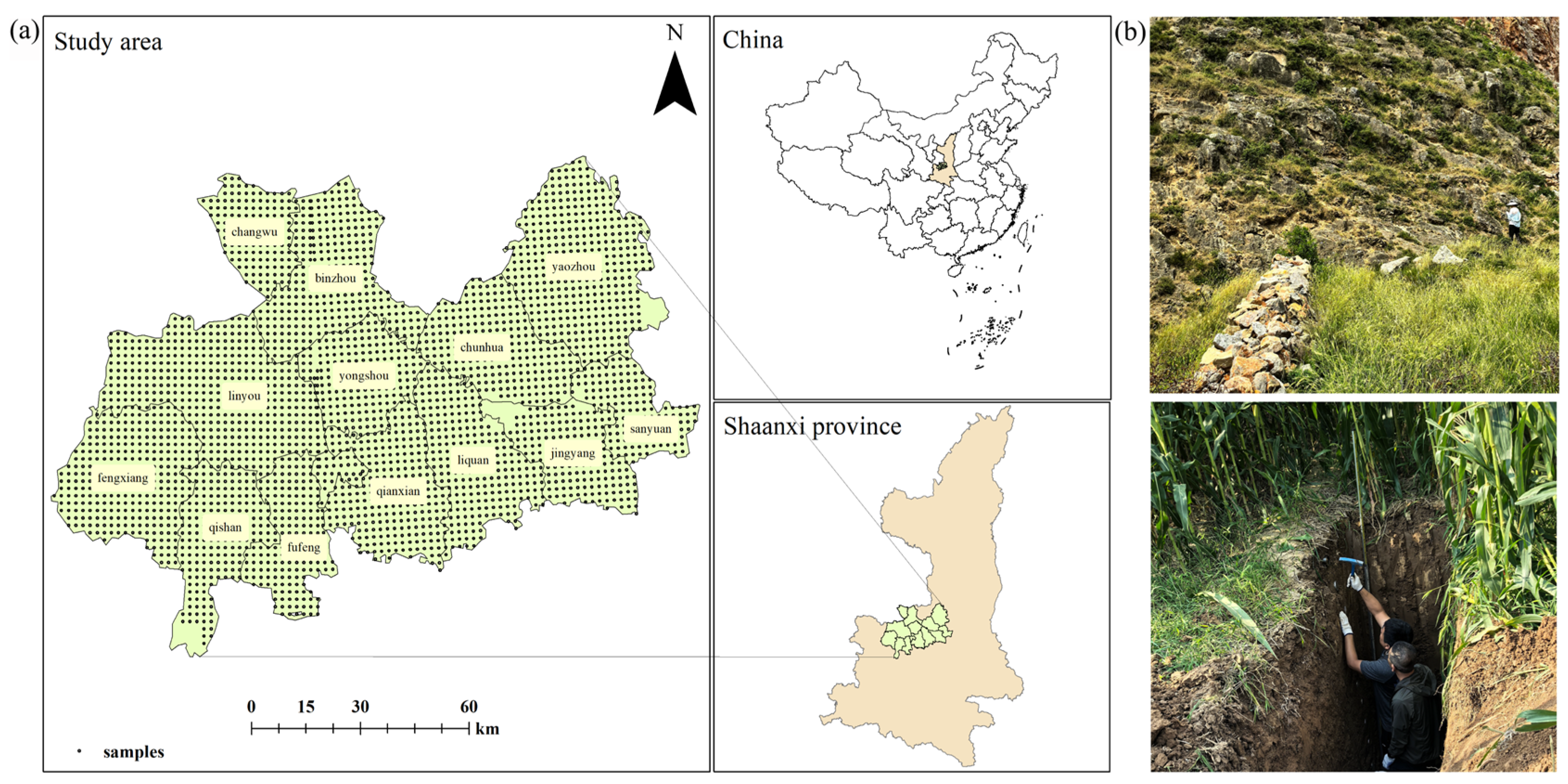
Figure 1. Study area and fieldwork scenes. (a) Geographical location of the study region, including its position in China, Shaanxi province, and a detailed map with sampling points; (b) Photographs of field-investigation activities.
Land 14 01609 g001
Figure 2. Model accuracy evaluation results. (a) Distribution of RMSE from 100-repeated five-fold cross-validation; (b) Scatter plot of predicted SIC values vs. independent validation observations.
Land 14 01609 g002
Figure 3. Spatial distribution of surface soil inorganic carbon (SIC) content in Weibei Loess region.
Land 14 01609 g003
Figure 4. Importance and significance of key covariates on surface SIC in Weibei Loess region using random forest model.
Land 14 01609 g004
Figure 5. Partial dependence plots between SIC and key driving covariates (srad, MAP, MAT, vs, NDVI, pH).
Land 14 01609 g005
Figure 6. Optimal parameter selection for variable discretization in the OPGD model.
Land 14 01609 g006
Figure 7. Interactive force of each driver (q-value).
Land 14 01609 g007
Figure 8. Risk area detection results.
Land 14 01609 g008
Table 1. Summary of environmental variables and their data sources.
Environmental FactorCovariatesDescription/UnitData Source
Climaticsrad, MAP, MAT, vpd, vs (continuous variable)Shortwave radiation (W/m2),
annual precipitation (mm),
mean temperature (°C),
vapor pressure deficit (kPa),
wind speed (m/s)
TerraClimate dataset, via Google Earth Engine (raster format, ~4 km resolution)
Topographicelevation, slope, aspect (continuous variable)Elevation (m),
slope (°),
slope direction
https://www.gscloud.cn, accessed on 4 January 2025 (raster format, 90 m resolution)
Vegetation-relatedNDVI (continuous variable)Normalized Difference Vegetation Indexhttps://ladsweb.modaps.eosdis.nasa.gov, accessed on 4 January 2025 (raster format, 1 km resolution)
vegetation type (categorical variable)Vegetation classificationhttps://lpdaac.usgs.gov/products/mcd12q1v006, accessed on 4 January 2025 (raster format, 500 m resolution)
Landscape (categorical variable)Broad landscape classification (e.g., loess hills, river valley, plateau)https://www.resdc.cn/data.aspx?DATAID=124, accessed on 4 January 2025 (vector format)
Soil PropertiespH (continuous variable)Field-measured soil acidityMeasured in field/lab then interpolated to study area by kriging
soil type (categorical variable)Soil classificationhttps://www.resdc.cn/data.aspx?DATAID=145, accessed on 4 January 2025 (vector format)
AnthropogenicNightlight (continuous variable)Nighttime light intensity (proxy for human activity)https://www.resdc.cn/DOI/DOI.aspx?DOIID=105, accessed on 4 January 2025 (raster format, 500 m resolution)
Table 2. Two-Stage Covariate Selection and Model Performance Summary.
CovariatesVIF #
(Round 1)
VIF
(Round 2)
VIF
(Round 3)
VI *
(Round 1)
VI
(Round 2)
VI
(Round 3)
aspect1.0041.0041.0010.001removedremoved
elevation24.583removed &removedremovedremovedremoved
landscape2.2102.2022.1880.0170.020removed
MAP6.4036.3665.5660.1180.1580.180
MAT31.58527.1418.3050.1030.1140.127
NDVI2.1582.0791.8350.0430.0460.045
nightlight1.7221.6811.6710.0230.026removed
pH1.3201.3191.3190.0250.0260.037
slope1.3561.3551.3540.006removedremoved
soiltype1.3081.2991.2980.0240.025removed
srad11.75111.1837.6310.1320.1710.193
vegetationtype1.3441.3131.2730.010removedremoved
vpd20.94420.325removedremovedremovedremoved
vs15.68810.40110.3170.0650.0750.106
R2 0.6210.6150.6030.6030.5970.590
MSE (g2/kg2) 0.1060.1070.1100.1100.1100.111
# VIF: Variance Inflation Factor. Values > 10 indicate significant multicollinearity; * VI: variable importance calculated by mean decrease in accuracy from the Random Forest model. Higher values indicate greater importance; : stepwise-selected variables, ensuring model accuracy (R2 and MSE) stayed within 5% of Round 1 maximum performance; &: the recalculated VIF or variable importance after the removal of the corresponding variable in each round.
Table 3. Model driving force size criterion of interval and interaction.
Criterion IntervalInteraction
q(X1 ∩ X2) < Min[q(X1), q(X2)]Nonlinear Weakening
Min[q(X1), q(X2)] < q(X1 ∩ X2) < Max[q(X1), q(X2)]Single-factor Nonlinear Weakening
q(X1 ∩ X2) > Max[q(X1), q(X2)]Two-factor Enhancement
q(X1 ∩ X2) = q(X1) + q(X2)Independent
q(X1 ∩ X2) > q(X1) + q(X2)Nonlinear Enhancement
Table 4. Contents of SIC in county (administrative unit) of the study area.
County (Administrative Unit)SIC Content (g/kg)
MinMaxRangeMeanStd
Yaozhou0.152.342.191.240.46
Fengxiang0.262.912.640.840.22
Linyou0.301.751.450.950.22
Fufeng0.341.871.530.900.22
Qishan0.101.591.490.710.25
Binzhou0.512.281.771.450.28
Chunhua0.302.722.421.490.30
Changwu0.931.880.951.530.17
Liquan0.983.562.581.580.35
Yongshou0.342.131.791.440.32
Jingyang1.072.741.681.510.22
Qianxian0.792.231.441.480.25
Sanyuan0.841.861.021.290.18
Disclaimer/Publisher’s Note: The statements, opinions and data contained in all publications are solely those of the individual author(s) and contributor(s) and not of MDPI and/or the editor(s). MDPI and/or the editor(s) disclaim responsibility for any injury to people or property resulting from any ideas, methods, instructions or products referred to in the content.