Article

Regional Ecological Environment Quality Prediction Based on Multi-Model Fusion

by
Yiquan Song
1,
Zhengwei Li
1,* and
Baoquan Wei
2
1
Department of Geography, Tianjin Normal University, Tianjin 300387, China
2
National Marine Environmental Monitoring Center, Dalian 116023, China
*
Author to whom correspondence should be addressed.
Land 2025, 14(7), 1486; https://doi.org/10.3390/land14071486
Submission received: 12 June 2025 / Revised: 9 July 2025 / Accepted: 14 July 2025 / Published: 17 July 2025

Abstract

Regional ecological environmental quality (EEQ) is a vital indicator for environmental management and supporting sustainable development. However, the absence of robust and accurate EEQ prediction models has hindered effective environmental strategies. This study proposes a novel approach to address this gap by integrating the ecological index (EI) model with several predictive models, including autoregressive integrated moving average (ARIMA), convolutional neural network (CNN), long short-term memory (LSTM), and cellular automata (CA), to forecast regional EEQ. Initially, the spatiotemporal evolution of the input data used to calculate the EI score was analyzed. Subsequently, tailored prediction models were developed for each dataset. These models were sequentially trained and validated, and their outputs were integrated into the EI model to enhance the accuracy and coherence of the final EEQ predictions. The novelty of this methodology lies not only in integrating existing predictive models but also in employing an innovative fusion technique that significantly improves prediction accuracy. Despite data quality issues in the case study dataset led to higher prediction errors in certain regions, the overall results exhibit a high degree of accuracy. A comparison of long-term EI predictions with EI assessment results reveals that the R2 value for the EI score exceeds 0.96, and the kappa value surpasses 0.76 for the EI level, underscoring the robust performance of the integrated model in forecasting regional EEQ. This approach offers valuable insights into exploring regional EEQ trends and future challenges.

1. Introduction

Regional ecological environmental quality (EEQ) refers to the ability of an ecosystem to sustain human life and support sustainable socioeconomic development in a given area [1,2,3]. It reflects ecosystem functioning, biodiversity, and human activities. EEQ is crucial for achieving sustainable development, human health, ecological protection, regional coordination, and public engagement in environmental matters [1,4,5]. Global climate change and human activities have caused significant EEQ changes across regions. Therefore, the dynamic assessment and prediction of EEQ are essential for the early detection of environmental trends and anomalies, supporting ecological health, and ensuring alignment between ecological stability and human progress.
Multiple EEQ assessment models, which are based on various frameworks, such as pressure-state-response and ecological footprints, have been developed and widely implemented [1,6,7,8]. One such model is the ecological index (EI), as outlined in China’s Technical Criterion for Ecosystem Status Evaluation (HJ 192–2015) (TCESE 2015) [8]. This model integrates a set of key indicators to assess regional EEQ, including parameters such as biodiversity, soil quality, water quality, and vegetation cover. The EI formula combines these indicators and utilizes normalization coefficients to assign appropriate weights and define the interrelationships among the indicators, thus serving as a standardized framework for regional EEQ evaluation in China. In recent years, China’s ecological environment departments have used the EI to release regional EEQ data, supporting environmental protection and management decisions. The EI model, which was initially dependent on statistical data at the county or provincial level, has undergone significant advancements with the integration of remote sensing (RS) data [4,5,9,10]. These developments have facilitated a transition to a more granular, pixel-level EEQ assessment mapping scheme. This evolution has markedly enhanced the precision and refinement levels of ecological assessments, enabling more accurate and detailed spatial analyses. Overall, backed by RS data and advanced quantitative methods, regional EEQ assessment models have matured to the point where they can effectively analyze ecological conditions and dynamic changes.
Prediction models are essential in various fields. These models typically rely on identifying patterns and trends from historical data to predict future outcomes, with data-driven statistical methods being the most commonly used model construction approaches [11]. Traditionally, statistical techniques, such as autoregressive integrated moving average (ARIMA) models, have been favored for their simplicity and interpretability [12]. However, as the complexity of data has increased, traditional methods have faced challenges, particularly in terms of capturing nonlinear relationships and handling high-dimensional data. With the advent of machine learning (ML), more sophisticated techniques, such as decision trees, support vector machines, and random forests, have emerged, yielding improved prediction accuracy by detecting complex patterns and nonlinear dependencies [13]. However, challenges such as feature selection and overfitting persist as data volumes expand. Deep learning (DL) techniques have significantly advanced predictive accuracy, particularly when handling large-scale, high-dimensional, and nonlinear data [14]. For example, long short-term memory (LSTM) networks have shown superior performance in processing time series data within the same spatial and systemic framework, effectively capturing long-term dependencies and making them especially effective for sequential data analyses in this context [15]. In addition to data-driven statistical models, system dynamics models, particularly cellular automata (CA), offer alternative prediction approaches [16,17]. Unlike traditional statistical methods, CA-based predictions are based on the evolution of local rules across a grid of cells, where the state of each cell is determined by the states of its neighbors and the associated transition rules [16,17]. These rules incorporate spatial dynamics (defining the positioning and spatial relationships of cells within the grid), territorial dynamics (characterizing the environmental context and spatial properties of the region each cell occupies), and environmental dynamics (accounting for external factors such as climate, resource availability, and other environmental variables that influence the evolution of cell behavior and interactions over time). This approach provides valuable insights into systems with complex interactions and emergent behaviors. Moreover, the integration of CA with ML and DL methods has started to enhance the predictive power of models by combining the strengths of both approaches—the capacity of CA modeling spatial and temporal dynamics and the ability of ML and DL to learn from large datasets [16,18]. Overall, prediction models are becoming increasingly accurate, efficient, and robust.
Although significant progress has been made regarding the development of prediction models and EEQ assessment models, research on EEQ prediction model is still underdeveloped. Some scholars have recognized the importance of EEQ prediction and have conducted preliminary studies using several methods, such as the gray forecasting model and CA-Markov model [2,19]. These approaches typically rely on time series EEQ data to predict future environmental quality levels. However, regional EEQ is a complex system influenced by multiple attributes and dimensions, with its evolution shaped by both natural environmental factors and socioeconomic drivers [3,20]. Consequently, EEQ prediction models that do not account for the interactions of these complex, multidimensional factors are limited in terms of accuracy and scientific rigor.
The accuracy of regional EEQ assessments depends heavily on the availability of precise input data. If the input data can effectively describe future scenarios, EEQ assessment models can theoretically predict future EEQ with high accuracy. In other words, when the input data accurately reflect future trends, EEQ assessment models gain predictive capabilities. Significant research has been devoted to predicting EEQ-related data, including land use/cover (LUC), normalized difference vegetation index (NDVI), and other environmental parameters [10,21]. Furthermore, studies that integrate LUC and NDVI to predict specific EEQ indicators have yielded promising results, often achieving high accuracy in their validation outcomes [17,22]. These efforts underscore the potential of combining multiple EEQ-related datasets to conduct regional EEQ predictions.
Building on the above foundation and addressing the gaps in EEQ prediction research, this paper introduces a multi-model fusion approach for regional EEQ prediction. The approach begins by analyzing the spatiotemporal evolution of the input data used to calculate the EI score, ensuring that both the temporal and spatial features of each dataset are considered. Based on this analysis, specific prediction models—such as ARIMA, LSTM, and CA—are selected and customized to capture the unique patterns within the data. After generating predictions from each model, the results are integrated into the EI model using a weighted fusion process. The final EI score is derived by applying normalization coefficients, accounting for the interdependencies and varying significance of each model’s contribution. This approach enhances prediction accuracy by leveraging the strengths of each model and aligning them with the underlying ecological data. Moreover, the approach is flexible and adaptable, making it suitable for evolving regional EEQ data and research requirements. Its adaptability ensures it can incorporate new insights, models, and datasets, making it an effective tool for future ecological assessments.

2. Study Area and Dataset

2.1. Study Area

Tianjin, a key city in northern China, covering 11,966.45 km2 was selected for this study. Tianjin governs 16 districts and is located at the confluence of the five major tributaries of the Haihe River, facing the Bohai Sea to the east and bordering the Yanshan Mountains to the north (Figure 1). The city’s flat terrain, with an average elevation of 3.5 m, features vast plains and some hilly areas in the north. Tianjin has a temperate, monsoonal climate with an average annual temperature of 12 °C. By 2024, its population reached 13.64 million, with an urbanization rate of 85.49%. Owing to policy support, industrial upgrades, and infrastructure development, Tianjin has experienced significant economic growth in recent years. However, this progress has also introduced a range of persistent ecological and environmental challenges [23,24]. These include air pollution caused by industrial emissions and traffic, water scarcity and contamination, and ecosystem degradation due to land development. In response, Tianjin has focused on expanding green spaces, improving air quality, and enhancing water resource management. Despite these efforts, striking a balance between economic growth and sustainable ecological development remains a critical challenge.

2.2. Dataset

The data used in this study included LUC, NDVI, soil erosion (SE), climatic, topographic, spatial distance, population, and statistical data (Table 1). The acquisition dates for all datasets were in October 2024. Except for the topographic data, the data collection period spanned from 2010 to 2022. The coordinate system used for all the datasets was GCS_WGS_1984, with the projection set to the Albers equal-area conic projection. To facilitate EEQ calculations, all datasets were resampled to a consistent spatial resolution of 30 m.
The LUC data were sourced from the dataset created by Jie Yang and Huang Xin [25]. This dataset was derived primarily from satellite imagery with a focus on Landsat data. In the study area, only seven categories were included: cropland, forest, shrub, grassland, water, barren, and impervious.
According to TCESE 2015 [8], the NDVI for EEQ assessment is based on the average of the maximum NDVI values from May–September. To obtain this information, monthly maximum NDVI data from the National Tibetan Plateau Data Center (TPDC), which were refined on the basis of Aqua/Terra MODIS MOD13Q1 data and LUC information, were initially retrieved [26]. Then, for each pixel, the maximum NDVI value for each of the five months (May–September) was extracted, and their average was calculated, ultimately producing the regional annual NDVI data.
SE data were obtained from the annual soil water erosion dataset for the Chinese mainland [27]. This dataset was constructed via Google Earth Engine and the revised universal soil loss equation.
The DEM from ASTER GDEM V3 [28] was used to derive four topographic variables: elevation (ELEV), slope (SLP), aspect (ASP), and the terrain ruggedness index (TRI). These variables were calculated using ArcGIS 10.5 software, which offers advanced spatial analysis tools and algorithms for precise terrain modeling.
Three climatic variables, including the annual mean temperature (TMP), annual mean precipitation (PRE), and annual mean potential evapotranspiration (PET), were employed in this study. Monthly data for these climate variables were obtained from the TPDC [29,30,31]. The TMP and PRE data were downscaled for China using the Delta method on the basis of global datasets acquired from CRU and WorldClim. A validation process implemented with data from 496 meteorological stations confirmed the reliability of the results. PET was calculated using the Hargreaves formula, which is based on China’s 1 km monthly temperature data (mean, minimum, and maximum).
Three spatial distance variables—distance to rivers (D2RV), distance to roads (D2RD), and distance to railways (D2RW)—were calculated based on the three feature layers (railways, roads and water) in OpenStreetMap (OSM) [32]. During this process, ArcGIS 10.5 software was used, and the Euclidean distance tool was applied.
The population density (PD) data were obtained directly from LandScan [33] and had a spatial resolution of 1 km.
The statistical data included 13 variables: chemical oxygen demand (COD), ammonia nitrogen (NH3), sulfur dioxide (SO2), smoke (dust) (YFC), nitrogen oxide (NOX), solid waste disposal (SOL), total annual precipitation (TAP), the GDP per capita (GDP/capita), the GDP of the tertiary industry (Tertiary GDP), water resources (WR), education financing expenditures (EFE), scientific and technological financing expenditures (STFE), and environmental protection financing expenditures (EPFE). These data were sourced from official statistics, including the Tianjin Binhai New Area Statistical Yearbook (https://tjj.tjbh.gov.cn/channels/11417.html, accessed on 25 October 2024), the Tianjin Statistical Yearbook (https://stats.tj.gov.cn/tjsj_52032/tjnj, accessed on 25 October 2024), and the Tianjin Water Resources Bulletin (https://swj.tj.gov.cn/zwgk_17147/xzfxxgk/fdzdgknr1/tjxx/index.html, accessed on 25 October 2024). The statistical data were incorporated into the attribute tables of the administrative boundary vector dataset and then converted into raster format.

3. Methods

3.1. Regional EEQ Assessment with the EI Model

According to TCESE 2015 [8], and considering the availability of data for the study area, the EEQ index is calculated using the EI model, which incorporates five key subindices: the habitat quality index (HQI), vegetation coverage index (VCI), water density index (WDI), land degradation index (LDI), and pollution load index (PLI) (Table 2). The EI results are presented in two forms: one is the EI score (ranging from 0 to 100), which quantifies the EEQ status with specific numerical values; the other is the EI level, where the EEQ is categorized into five classes—excellent, good, moderate, poor, and very poor—based on thresholds of 75, 55, 35, 20, and 0, respectively [8]. The spatial units for the regional EEQ assessment are defined as 500 m × 500 m. During the calculation process, the various subindices are integrated and weighted according to their relative significance, with the final EI score providing a comprehensive evaluation of the EEQ in the study area.

3.2. Regional EEQ Prediction and Evaluation

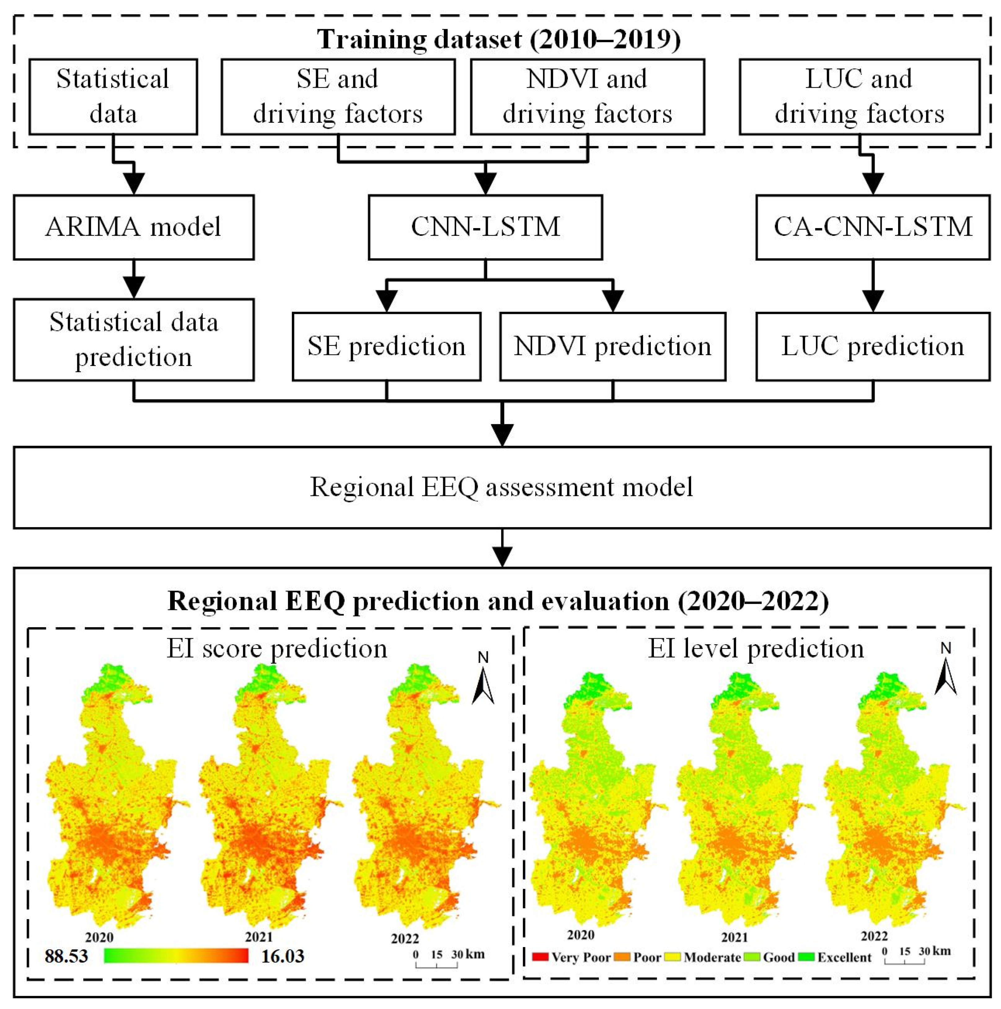
The regional EEQ prediction and evaluation framework is shown in Figure 2. First, the data used to calculate the EI score, as outlined in Table 2, are categorized into four types: LUC, NDVI, SE, and statistical data. For each data type, a specific prediction model is developed on the basis of the nature of the data by using the training dataset from 2000 to 2019. Specifically, statistical data are predicted using ARIMA, NDVI data are predicted using an integrated CNN-LSTM model, and LUC data are predicted with a CA-based model combined with CNN and LSTM. After training, these models are used to predict data for the period from 2020 to 2022. The resulting predictions are then input into the EI model, which integrates the individual predictions to assess the regional EEQ.

3.2.1. Statistical Data Prediction Using the ARIMA

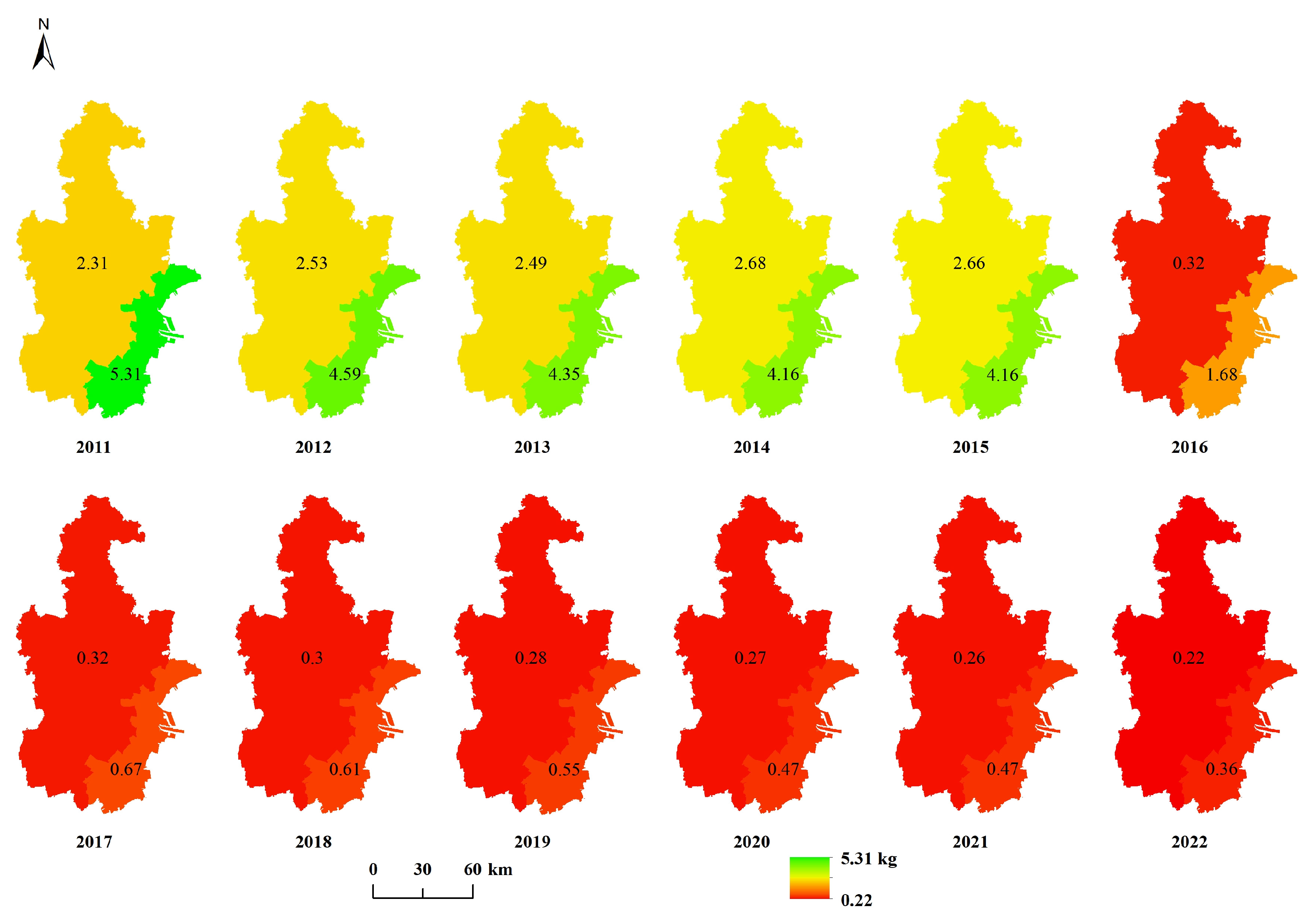
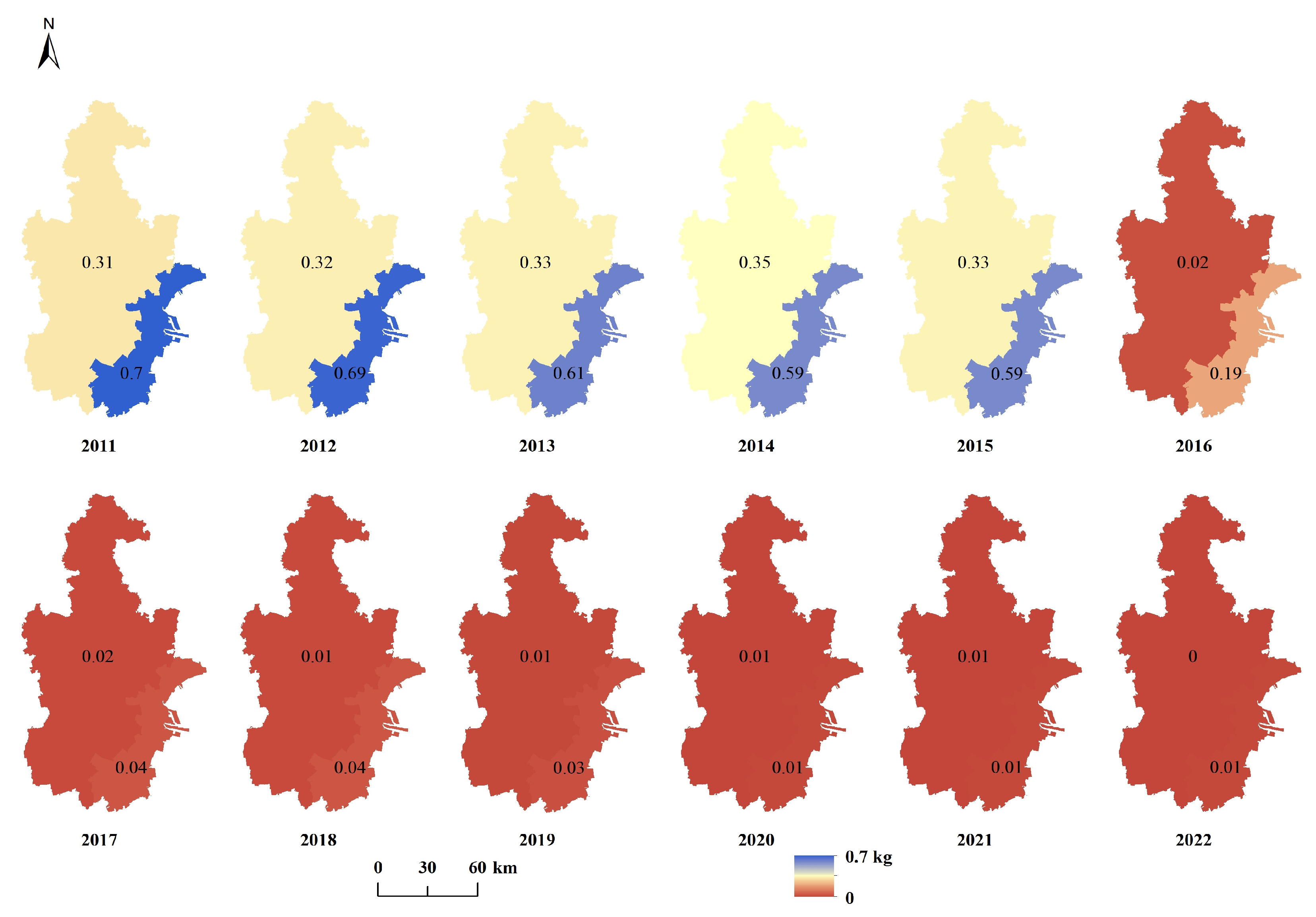
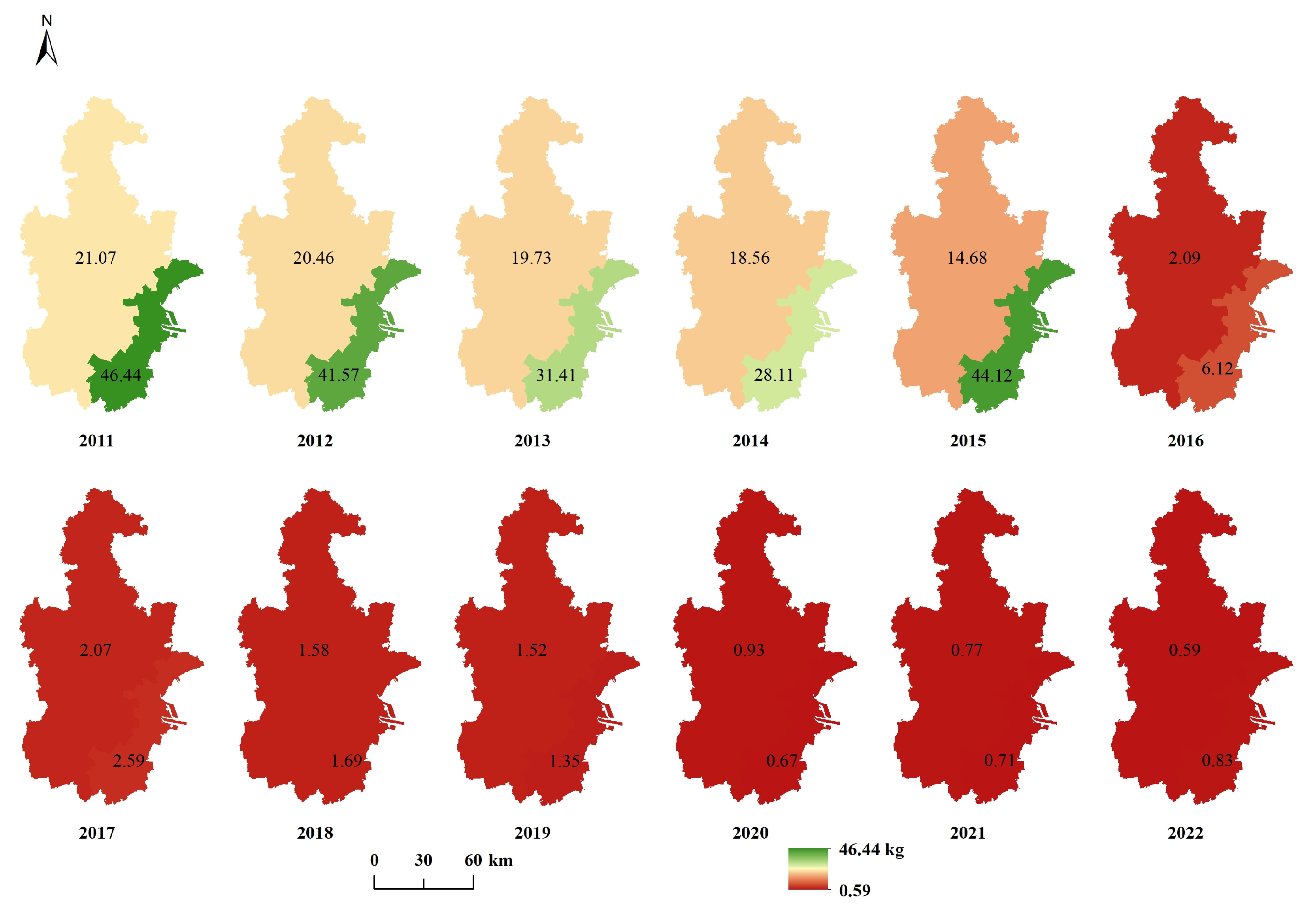
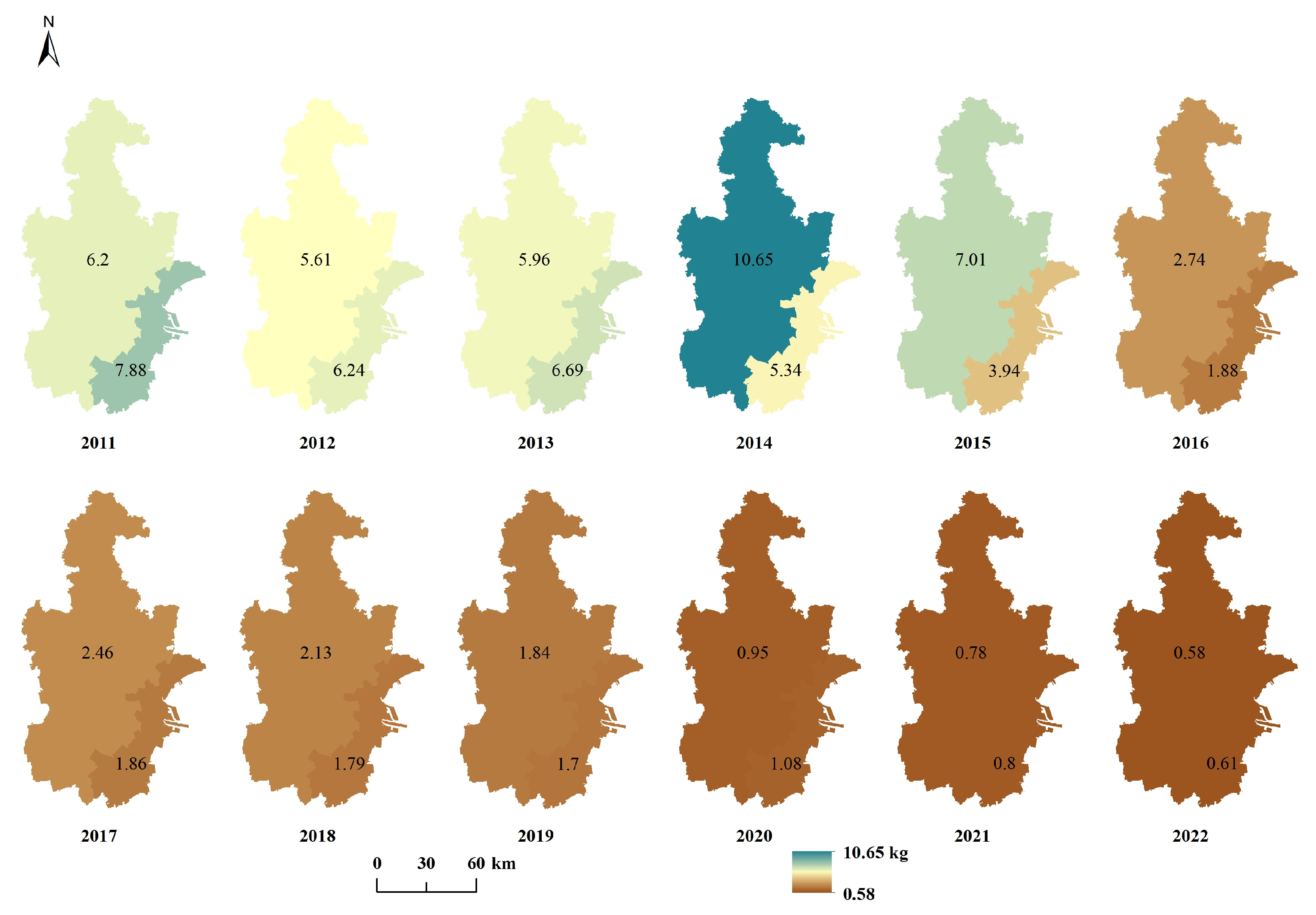
Statistical data are aggregated at the administrative unit level, which limits their spatial specificity. Moreover, the sample size is relatively small, with only one data point available per administrative unit each year (Figure A1, Figure A2, Figure A3, Figure A4, Figure A5, Figure A6 and Figure A7). In other words, the data lack strong spatial specificity and are constrained by a limited sample size. Given these characteristics, a traditional prediction model, the ARIMA, is employed (Figure 3).
The ARIMA model, which was introduced by Box and Jenkins in 1970, assumes that a time series can be approximated by a mathematical model to predict future values based on historical data [12]. It consists of three components: autoregressive (AR), integrated (I), and moving average (MA) parts. The AR part models the relationship between the current and past values, which is denoted by p. The I component addresses non-stationarity by differencing the input series, with d representing the number of differences. The steps for ARIMA modeling include the following: (1) testing for stationarity using plots, where if non-stationarity is observed, differencing is applied; (2) estimating the parameters p, d, and q using autocorrelation and partial autocorrelation plots; (3) fitting the model and ensuring that the residuals meet the white noise assumption; and (4) using the fitted model for forecasting future values.

3.2.2. NDVI and SE Prediction Using CNN and LSTM Models

The NDVI is a common numerical indicator for monitoring the distribution and growth of vegetation, whereas SE reflects quantifiable soil degradation data. In terms of temporal characteristics, the NDVI exhibits long-term trends with interannual fluctuations influenced by climate and weather patterns, whereas SE changes gradually over time, with cumulative effects becoming more evident over several decades. Although there are differences between the properties and temporal variation characteristics of the NDVI and SE data, both provide valuable insights into continuous geographic variables. Their prediction modeling challenges involve the use of comprehensive spatial and temporal analyses, and both methods share time series characteristics. The CNN-LSTM model combines the feature extraction ability of convolutional neural network (CNN) and the sequence modeling ability of LSTM, making it suitable for handling data with spatial and temporal dependencies. The CNN-LSTM model can extract nonlinear and complex patterns from data, which is highly useful for understanding and predicting the intricate evolutionary processes of the NDVI and SE. Therefore, a CNN-LSTM model is used in this study (Figure 4).
A CNN is a feedforward neural network that integrates convolutional operations within a deep structure, enabling adaptive self-learning and efficient feature extraction for classification and prediction tasks [34]. A typical CNN comprises three components: a convolutional layer, a pooling layer, and a fully connected layer. The convolutional layer uses filters to capture local features, such as edges and textures, whereas the pooling layer reduces the dimensionality and computational complexity of the data, preserving the key features. The fully connected layer then uses these features for classification or regression. In NDVI and SE prediction scenarios, CNNs extract complex spatial features at various scales, such as plant growth and vegetation density patterns, through convolution and pooling. These feature maps are passed into an LSTM model, which captures the long-term dependencies in the time series data. CNNs automatically learn spatial features, eliminating the need for manual feature extraction steps, and their pooling operations reduce image resolutions, lowering the incurred computational complexity while retaining essential information. This allows the LSTM model to process data more efficiently while preserving the key spatial details.
An LSTM model is a specialized form of a recurrent neural network (RNN) that is designed to model long-term dependencies in time series data [15]. Unlike traditional RNNs, LSTM models overcome vanishing and exploding gradients by using memory cells and gating mechanisms (input, forget, and output gates), which enhance their retention of historical information and improve the resulting prediction accuracy. The input gate controls the storage of the current input in the memory cell, the forgetgate determines how much of the existing information should be discarded, and the output gate regulates how much of the stored information is passed to the next layer or used for the final predictions. In NDVI and SE prediction tasks, LSTM models play a crucial role in two areas: (1) extracting temporal features and capturing long-term trends from the NDVI, SE and driving factor datasets and (2) modeling the complex nonlinear relationships between spatial and temporal features to effectively forecast NDVI and SE time series.

3.2.3. LUC Prediction Using a CA Model Coupled with CNN and LSTM Models

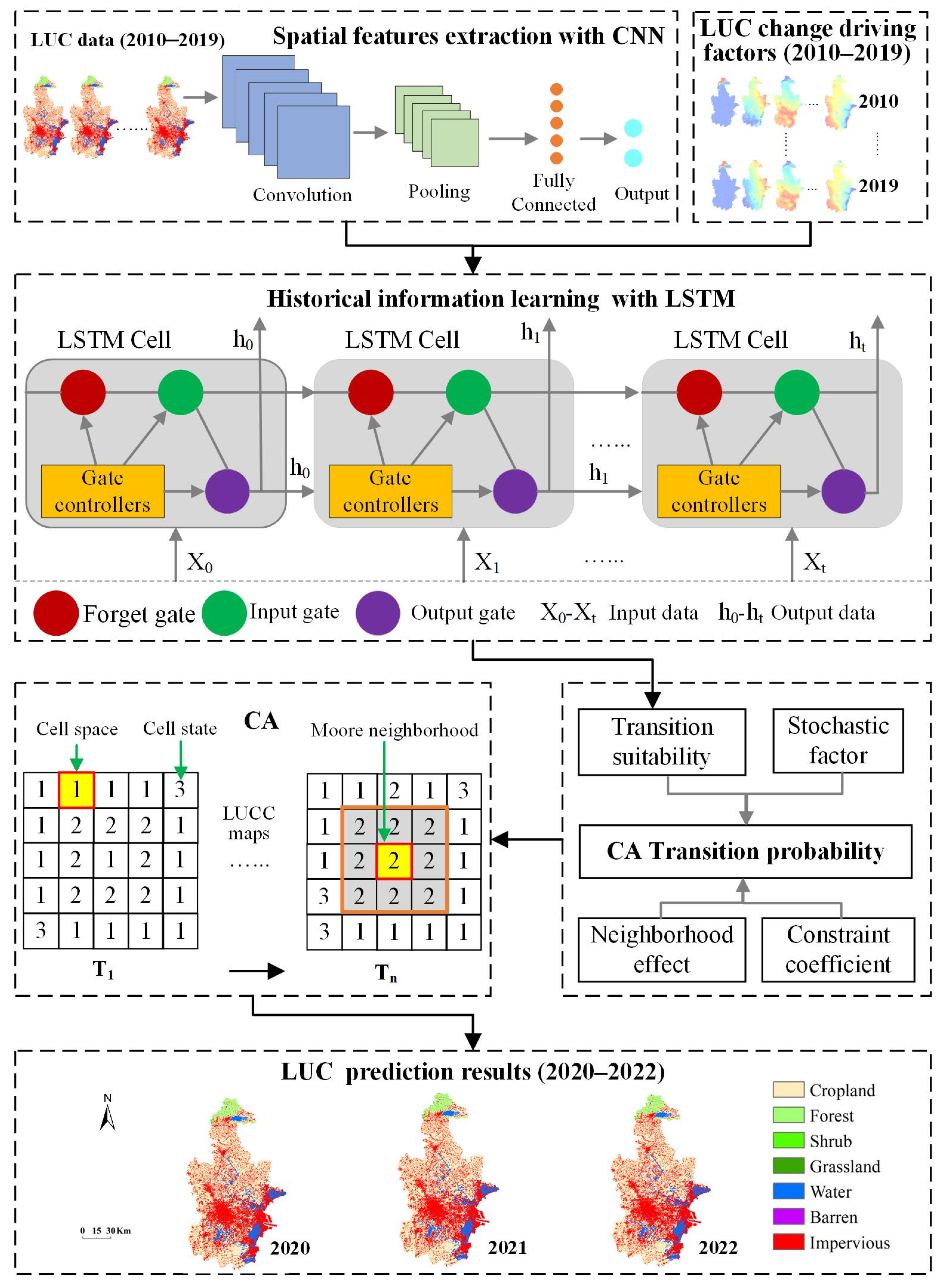
CA models have gained widespread use in LUC prediction settings because of their excellent scalability and ability to effectively account for spatial heterogeneity [16,17]. The basic framework of a CA model consists of five key components: the cell space, cell states, the neighborhood, time steps, and transition rules. Among these, the transition rules are the core aspects of CA models, as they determine how the LUC cell states evolve spatially and temporally. Each cell updates its state on the basis of the statuses of its neighboring cells and predefined local rules, thereby driving changes in the LUC data across the entire region. In CA-based LUC prediction scenarios, the transition rules typically include four key elements: transition suitability, neighborhood constraints, restrictive constraints, and random disturbances. Owing to the decisive role of transition rules in predictions, statistical models and ML models have been widely used in CA-based LUC prediction tasks to further optimize and refine transition rules, thereby providing improved prediction accuracy and model adaptability [16,17].
Although remarkable achievements have been made in terms of constructing the transition rules of CA models, the long-term temporal dependency issue involving LUC data and the inadequate representations of neighborhood effects still persist [18]. By integrating CNN and LSTM models into a CA model, it becomes possible to better capture complex spatial and temporal dependencies, enhancing the effectiveness and reliability of the CA transition rule construction process and thus improving the resulting prediction accuracy. On the basis of the relevant studies, designs an LUC prediction model that couples a CA model with both CNN and LSTM models (Figure 5) is designed in this paper. Similarly to the main functions of CNN and LSTM models in NDVI/SE prediction scenarios, the CNN primarily extracts complex spatial features at different scales and levels from LUC data through convolutional and pooling layers. The LSTM model, on the other hand, further extracts the temporal features of the LUC and driving factor datasets from the spatial features extracted by the CNN, applying the complex nonlinear relationships between the spatial and temporal features of the LUC data and LUC driving factors to calculate CA transition rules.
On the basis of the CA-CNN-LSTM model, the transition probability P of the CA cells in LUC is represented as follows:
P = Sij × Nij × Zij × Rij,
where Sij denotes the transition probability of cell (i,j) calculated using the CNN-LSTM model, Nij represents the neighborhood constraint, Zij is the global spatial location constraint, and Rij reflects the uncertainty in the state change process.

3.2.4. Evaluation Metrics

Considering that the predicted data include both continuous numerical variables (statistical data, NDVI, SE, and EI score) and discrete categorical variables (LUC and EI level), different evaluation metrics are employed in this paper to assess the accuracy and reliability of the prediction results (Table 3). For continuous numerical data, the evaluation criteria include the root mean square error (RMSE), mean absolute error (MAE), mean absolute percentage error (MAPE), and coefficient of determination (R2). For discrete categorical data, the evaluation criteria include the overall accuracy (OA) and the kappa coefficient.

4. Model Implementation and Experimental Results

4.1. Model Implementation

SPSS 25.0 is employed to implement the ARIMA model for predicting the statistical data. The stationarity of the time series is evaluated using the augmented Dickey-Fuller (ADF) test [12]. To optimize the model, autocorrelation function (ACF) and partial autocorrelation function (PACF) plots are analyzed to determine the appropriate values for the model parameters (p, d, and q) [12].
The CNN-LSTM model for predicting the NDVI and SE is developed using TensorFlow in Python 3.6 leveraging several libraries, such as Keras, scikit-learn, GDAL, Pandas, and NumPy [35]. The CNN part consists of six layers: two convolutional layers, two pooling layers, one fully connected layer, and one activation layer. The first convolutional layer uses 32 filters (6 × 6), whereas the second layer uses 64 filters (3 × 3). The pooling layers employ 3 × 3 max pooling. ReLU activation is used in the convolutional and fully connected layers, and linear activation is applied in the output layer for regression tasks [34]. The LSTM part includes two LSTM layers and two dropout layers (dropout rate = 0.3) to prevent overfitting, with linear activation in the LSTM layers. This model is designed for single-step prediction to forecast NDVI and SE values, making it well suited for regression-based forecasting. The prediction process incorporates climate (TEM and PRE), terrain (ELEV, ASP, SLP, and TRI), and spatial distance-related variables (D2RW, D2RD, and D2RV) as driving factors.
The LUC prediction model shares a similar development environment with the NDVI/SE prediction model, but the LUC task involves multiclass classification, where each pixel represents a discrete land use type, whereas NDVI/SE is a regression task with continuous values. These differences necessitate distinct adjustments to the CNN-LSTM model. The CNN design includes a fully connected layer with 7 neurons, each corresponding to a specific LUC type in the study area, which enhances the resulting classification accuracy. The output layer employs a softmax activation function to handle the multiclass classification task, calculates the probability distribution across categories and enables the model to select the most likely LUC type. To achieve improved accuracy and generalizability, data augmentation techniques (such as rotation, translation, and cropping) and regularization methods (including dropout and L2 regularization) are used to prevent overfitting and enhance the robustness of the model. The categorical cross-entropy loss function optimizes multiclass predictions, improving the ability of the model to distinguish between different LUC types. In the CA model, transition probabilities are influenced by neighborhood effects, which are based on the frequency of the pixel values in a 3 × 3 neighborhood. A random factor, which is generated by random numbers between 0 and 8, introduces stochasticity in the LUC change process. Restriction factors control the overall change trend, adjusting the results when neighborhood influences do not align with development probabilities. The prediction procedure incorporates a range of driving factors, including climate (TEM and PRE), terrain (ELEV, ASP, SLP, and TRI), spatial distance-related variables (D2RW, D2RD, and D2RV); population data; and statistical data (GDP, GDP/capita, tertiary GDP, EFE, STFE, and EPFE).

4.2. Model Performance and Analysis

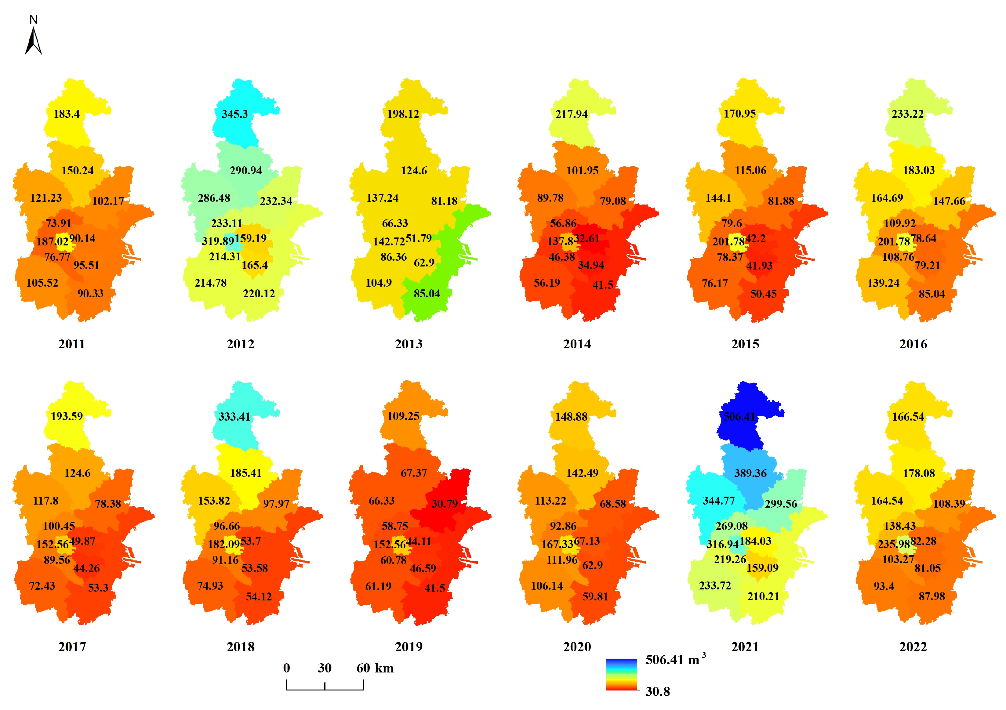
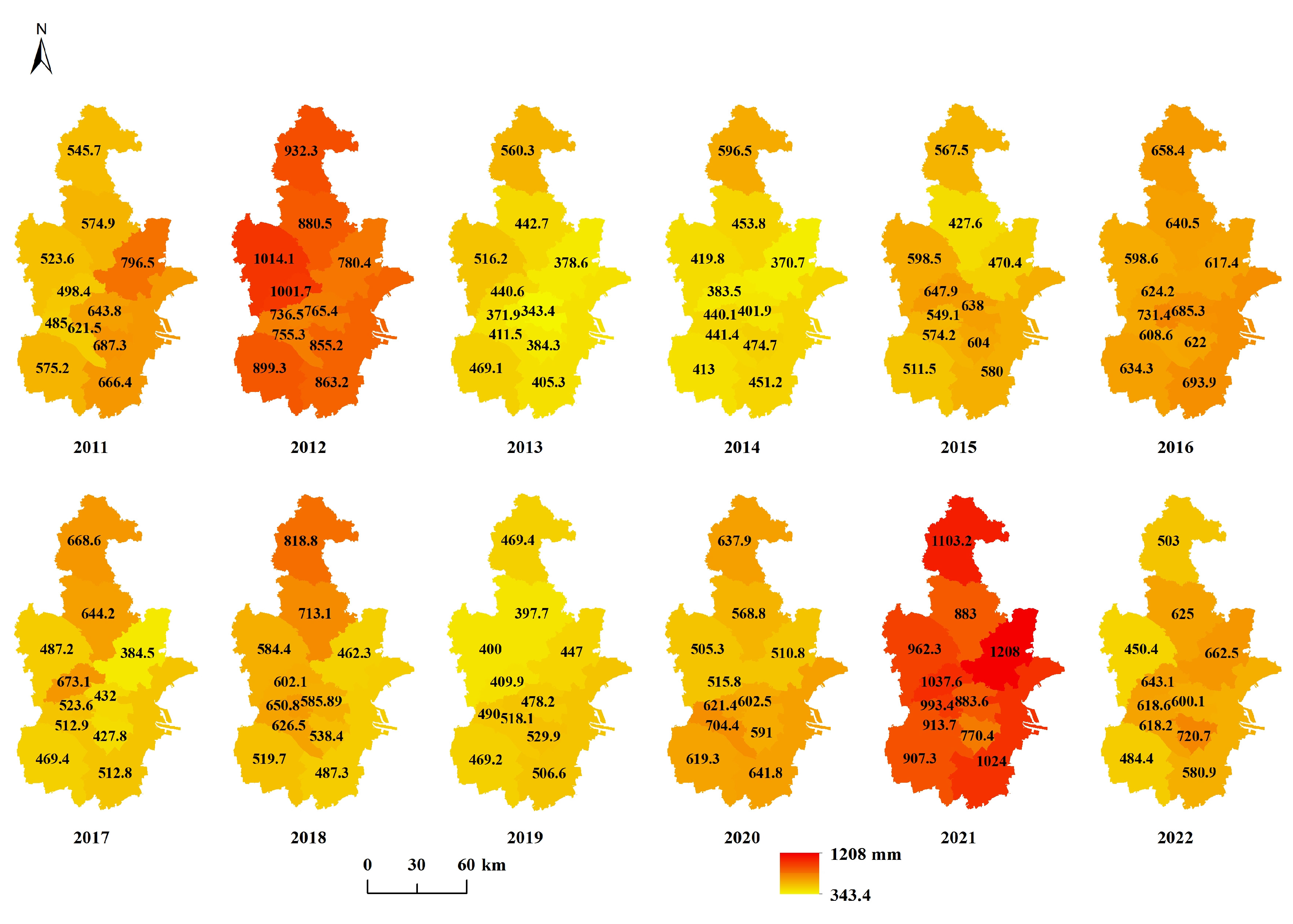
Table 4 shows that the overall prediction performance of the statistical data is satisfactory, with most data points exhibiting MAPEs below 25, suggesting that the ARIMA model generally fits the data well. However, owing to the inherent variability in the data values (Figure A1, Figure A2, Figure A3, Figure A4, Figure A5, Figure A6 and Figure A7), the RMSE and MAE significantly fluctuate. Notably, the MAPE prediction errors induced for WR and NH3 are prominent. A further analysis reveals that the TAP data displayed considerable fluctuations during the forecast period, particularly in 2021, when the actual value reached 1103.2 mm, which was significantly greater than the long-term average of approximately 600 mm (Figure A7). This anomaly underscores the limitations of the ARIMA model in terms of accurately predicting extreme events. As a result, the overall predictions produced for WR and TAP are less accurate. Additionally, the COVID-19 pandemic (2020–2023) caused industry disruptions, reducing production and affecting pollutant emissions. These changes led to abnormal fluctuations in the data, making the prediction process more difficult and reducing the accuracy of some models.
The LUC, NDVI, and SE prediction models demonstrate robust performance in terms of prediction accuracy and stability, as indicated by the metrics shown in Table 5 and Table 6. The NDVI prediction model consistently achieves RMSEs below 0.07, MAEs under 0.05, MAPEs under 25, and an R2 values greater than 0.82 (approaching 0.9), suggesting high precision and stability in its predictions. The SE prediction model, while slightly less accurate than the NDVI, maintains RMSEs below 1.7 and R2 values of approximately 0.8, reflecting a solid predictive ability. The LUC prediction model has kappa coefficients above 0.94 and OA values exceeding 0.96, indicating exceptional classification accuracy. Overall, the LUC prediction model outperforms the other models, followed by the NDVI prediction model, with the SE prediction model showing lower performance. These performance discrepancies can be attributed to several factors. (1) LUC changes tend to follow long-term, more predictable trends influenced by factors that may exhibit varying levels of stability over time, such as climate change, socioeconomic activities, and land management policies, which make them more predictable to some extent. In contrast, the NDVI and SE are more affected by short-term, dynamic factors (e.g., seasonal weather variations and soil properties), which introduce higher levels of variability and reduce the accuracy of prediction. Although the performance of the NDVI model is comparable to that reported in previous studies, it remains less accurate than the LUC prediction model. (2) The SE prediction process is particularly sensitive to the complex interactions of local topography, precipitation patterns, and LUC changes, making it challenging for CNN-LSTM models to effectively capture these intricate relationships. Furthermore, the spatial distribution of soil erosion is highly heterogeneous, with some areas experiencing severe erosion and others remaining unaffected, complicating the ability of the model to learn from sparse or imbalanced data. In contrast, the NDVI benefits from a wealth of RS data, enabling the model to capture finer spatial features, thereby improving its prediction accuracy. These factors contribute to the relatively low performance of the SE prediction model relative to that of the NDVI model. Finally, as observed in the similar multistep LUC and NDVI predictions, prediction errors tend to accumulate and magnify over time due to temporal data resolution limitations, leading to increased uncertainties and errors in the long-term forecasts.
According to Table 7, the EI prediction model shows high predictive accuracy. Specifically, the RMSE of the EI score is consistently less than 2.65, the MAE is less than 1.95, the MAPE is less than 5, and the R2 is close to 1, indicating strong prediction performance. However, the predictive accuracy of the EI level is slightly lower, with an OA below 0.95 and a kappa coefficient just above 0.75. This may be due to the classification intervals used for the EI level, where small differences in the EI score can lead to reduced classification accuracy. Compared with those of the subindices, the MAPE of the EI score is lower than those of the NDVI and statistical data, and its R2 is higher than those of the NDVI and SE, suggesting that incorporating multiple subindices into the EI score results in more accurate predictions. In contrast, the predictive accuracy of the EI level is somewhat lower than those of some contributing factors, as evidenced by its kappa coefficient and OA, which are lower than those of LUC.
To investigate the spatiotemporal distribution characteristics of the EI error, the absolute difference (ΔE) between the true and predicted EI score values is computed annually for each spatial EEQ assessment unit (Figure 6). The analysis indicates an uneven spatiotemporal distribution of ΔE within the study area. While most regions exhibit relatively low ΔE values, several areas display significantly greater errors. Notably, regions with ΔE > 10 exhibit pronounced spatial clustering patterns, which remain consistent across years, suggesting that the predictive accuracy of the model is constrained in these specific areas. A geospatial analysis of the study area reveals that these high-error regions are primarily concentrated around the Beidagang Wetland, Tuanbo Lake, the Jiyun River in Ninghe District, and the catchment areas of the Chao Bai New River and Yongding New River.

4.3. Exploring the Causes of EI Prediction Errors

To better understand the error distribution and the relative importance of each subindex in the EI score prediction error, the total absolute error (AE_Value) of the EI score and its subindices, along with the dominant subindex contributing to the EI score error (DI_Count), is calculated for each spatial unit within the study area, including regions with high EI errors (ΔE > 10) (Table 8 and Table 9). A comprehensive error calculation method is used to quantify the contribution of each subindex to the total EI error. In this approach, the absolute errors of each subindex are weighted by the corresponding coefficients used in the EI calculation formula. For each spatial unit, the subindex with the greatest error contribution is identified as the dominant error index for that unit. This method provides insights into the underlying factors driving the errors in the EI score predictions.
By comparing Table 8 and Table 9, the following conclusions can be drawn. (1) The AE_Value and DI_Count of the VCI consistently exhibit the highest values among all the subindices of the EI in the study area, indicating that the VCI is the primary source of the EI error within the region. This could be attributed to the relatively low simulation accuracy of the NDVI in the area. However, in regions with ΔE > 10, the AE_Value of the VCI decreases significantly, decreasing to less than 1.7% of its original value. This further suggests that the error induced across spatial units in the NDVI simulation is relatively uniform, with fewer high errors. (2) While the AE_Value and DI_Count of the HQI are lower than those of the other subindices in the study area are, the HQI consistently has the highest AE_Value in regions with ΔE > 10. This suggests that despite the relatively high simulation accuracy of LUC changes, there are certain regions where substantial LUC change simulation errors exist. These errors are the primary contributors to the high EI errors observed in those areas.
To further explore the causes of high EI errors (ΔE > 10), a comparative analysis is conducted on the spatial distributions of the key subindexes contributing to EI errors, RS imagery (sourced from Esri World Imagery Wayback, https://livingatlas.arcgis.com/wayback, accessed on 25 October 2024), and LUC and NDVI data (Table 2). The comparison reveals that the main factors behind the high EI errors are several issues related to multitemporal data discrepancies. (1) Inconsistencies in LUC wetland classification are the main cause of the high errors in the HQI. For example, the Beidagang Wetland showed significant discrepancies between the 2019 and 2020 data. Some areas classified as cropland in 2019 were classified as water in 2020 (Figure 7a–c). However, the Beidagang wetland has remained stable over the past two decades. These inconsistencies are due to natural processes, such as water-land alternations, reed and vegetation growth, and seasonal hydrological changes, which affect spectral features and complicate the classification of RS imagery. As a result, the errors in LUC prediction models lead to inaccuracies in EEQ predictions. (2) Fluctuations in the NDVI also occur. At certain water bodies and water-land interfaces, the influences of multiple complex factors, including hydrological conditions, aquatic vegetation, and climatic changes, result in significant fluctuations in the NDVI values (Figure 7d–g). These fluctuations create temporal inconsistencies across different years, undermining the stability of the predictions and contributing to high errors in the VCI simulations. (3) Abrupt LUC type transitions pose another challenge, especially in areas affected by human activities, such as the conversion of natural land into impervious surfaces (Figure 7h–k). These sudden LUC changes are difficult to predict and cause large deviations in the LUC or NDVI simulation results, leading to significant discrepancies in the LDI or VCI values.

5. Discussion

A robust and accurate regional EEQ prediction model is crucial for effective ecological management and sustainable development [2,19]. However, the design and implementation of such a model face several critical challenges, including data quality and availability, the integration of complex ecological and socio-economic variables, and the inherent uncertainty in long-term predictions. This study primarily focuses on the design of the framework for the regional EEQ prediction model and the development of corresponding implementation methodologies, aiming to overcome the limitations of previous models.
Considering that regional EEQ assessment models have reached a relatively mature stage, and these models exhibit a certain degree of predictive capability, with the contributions of various factors to EEQ being well-established, this study builds upon existing EEQ assessment frameworks to develop an advanced predictive model. The key strength of the proposed framework lies in its ability to integrate a range of influencing factors, including both spatial and temporal dynamics, into a cohesive model. This integration significantly enhances the accuracy and reliability of predictions. By leveraging established ecological models, the framework effectively addresses the complex interactions between diverse ecological variables, overcoming the limitations of previous models that often failed to capture the intricate relationships between these factors [2,19]. The case study demonstrates that the proposed prediction method delivers exceptional performance in terms of accuracy, validating its feasibility and practical applicability for regional EEQ prediction tasks. While this paper primarily focuses on regional EEQ prediction using the EI model, the proposed framework and methodology are equally applicable to other regional EEQ assessment models. This finding suggests that the proposed prediction approach is highly scalable, allowing it to adapt flexibly to the ecological characteristics of different regions and meet the specific data requirements of various models.
Considering the spatiotemporal characteristics of the data in calculating the EI value, as well as the inherent features of existing predictive models, the EEQ prediction model was implemented using a multi-model fusion approach. This methodology integrates the strengths of multiple models to more accurately capture the complex dynamics of ecological environments and enhance predictive performance. For NDVI and SE data, a hybrid approach combining CNN and LSTM models is proposed. LSTM models are particularly effective at handling time-series data and capturing its temporal features, while CNNs excel at extracting spatial patterns and recognizing underlying structures in the data [14,18]. The combination of CNN and LSTM models enables the model to better understand the spatiotemporal variations in the NDVI and SE, as well as their complex interactions with environmental factors, thereby improving the resulting prediction accuracy. For LUC data, CA is further integrated with both LSTM and CNN models to construct a comprehensive model for predicting and forecasting LUC evolution trends. CA, through neighborhood rules and interactions, effectively predict spatial distributions and trends in LUC changes, thus enhancing the ability of the model to predict spatiotemporal dynamics [16,17]. For statistical data, the ARIMA model is employed due to its effectiveness in capturing temporal dependencies and trends, even when only limited historical data is available [12]. Despite substantial progress in model implementation, several key areas still require optimization, particularly in the fine-tuning of hyperparameters for the LSTM and CNN models. These refinements are crucial for improving the forecasting performance and overall effectiveness of the predictive model [34,35]. Furthermore, it is important to note that other predictive models, may also demonstrate strong performance in forecasting NDVI, SE, LUC, and statistical data [16,17,18,22]. Therefore, a comprehensive and systematic evaluation of various modeling techniques will be essential in future research to identify the most effective methods for each specific task.
Moreover, data quality and availability also have significant effects on prediction outcomes. High-quality data not only improve the effectiveness of the model training process but also enhance its generalizability in applications. While the dataset used in this study are relatively reliable, contributing to improved model performance in training and prediction, inevitable errors and inconsistencies remain [25,29,30,31]. In the case study, wetland classification errors within the LUC data and temporal-spatial fluctuations in the NDVI have led to high prediction error. To overcome these challenges, integrating data processing techniques, such as data cleaning, into the prediction process is essential for enhancing the accuracy and reliability of the results [36]. Furthermore, the calculation of the EI value is related to statistical data. However, traditional statistical datasets are often confined to regional statistics, which fail to capture regional heterogeneity when EEQ calculations are performed at a finer spatial scale. With the rapid advancement of big data and AI technologies, spatialized processing of statistical data has become an emerging trend, leading to the development of more spatially detailed data products [37]. Future research should fully integrate spatialized statistical data with corresponding predictive models to obtain more accurate and reliable regional EEQ predictions.

6. Conclusions

Regional EEQ assessment and prediction are crucial for environmental management and supporting sustainable development [2,19]. To address the limitations in EEQ prediction, a novel method has been designed and implemented that integrates the EI model with CNN, LSTM, CA, and ARIMA. Through case data collection and analysis, the reliability of the prediction model has been validated, demonstrating its capacity to synthesize various ecological factors while maintaining flexibility and scalability for broader applications. The core contribution of this approach lies in harmonizing the strengths of different methodologies: (1) CNN and LSTM models for capturing spatial-temporal dependencies and nonlinear patterns in NDVI, SE, and LUC changes; (2) CA for predicting localized LUC transitions; (3) ARIMA for modeling temporal trends in statistical data; and (4) the EI model for integrating diverse prediction results from the aforementioned methodologies to generate a comprehensive regional EEQ prediction.
Challenges remain, especially regional prediction accuracy disparities due to data limitations, highlighting the need for stronger data quality assurances. Future research should focus on advanced data preprocessing, outlier detection, and cross-validation approaches to mitigate data uncertainties [36]. Furthermore, while the regional EEQ prediction framework shows adaptability, its generalizability requires validation through large-scale prediction tasks conducted across diverse regions to assess its performance under varying environmental stressors. Additionally, further exploration and integration of advanced DL models to enhance the accuracy and robustness of EEQ prediction are necessary. For example, models such as deep reinforcement learning, graph neural networks (GNN), and attention-based architectures like transformers have shown remarkable potential in capturing complex nonlinear interactions and high-dimensional spatial-temporal dependencies [38,39]. These models could significantly improve the predictive performance of EEQ by effectively synthesizing diverse, multi-source data.

Author Contributions

Conceptualization, Y.S.; methodology, Y.S.; software, Z.L.; validation, Z.L.; formal analysis, Y.S.; investigation, Y.S.; resources, Y.S.; data curation, Z.L.; writing—original draft preparation, Y.S.; writing—review and editing, Y.S. and B.W.; visualization, Y.S.; supervision, Y.S.; project administration, Y.S. All authors have read and agreed to the published version of the manuscript.

Funding

This research received no external funding.

Data Availability Statement

The original contributions presented in the study are included in the article, further inquiries can be directed to the corresponding author.

Conflicts of Interest

The authors declare no conflicts of interest.

Appendix A

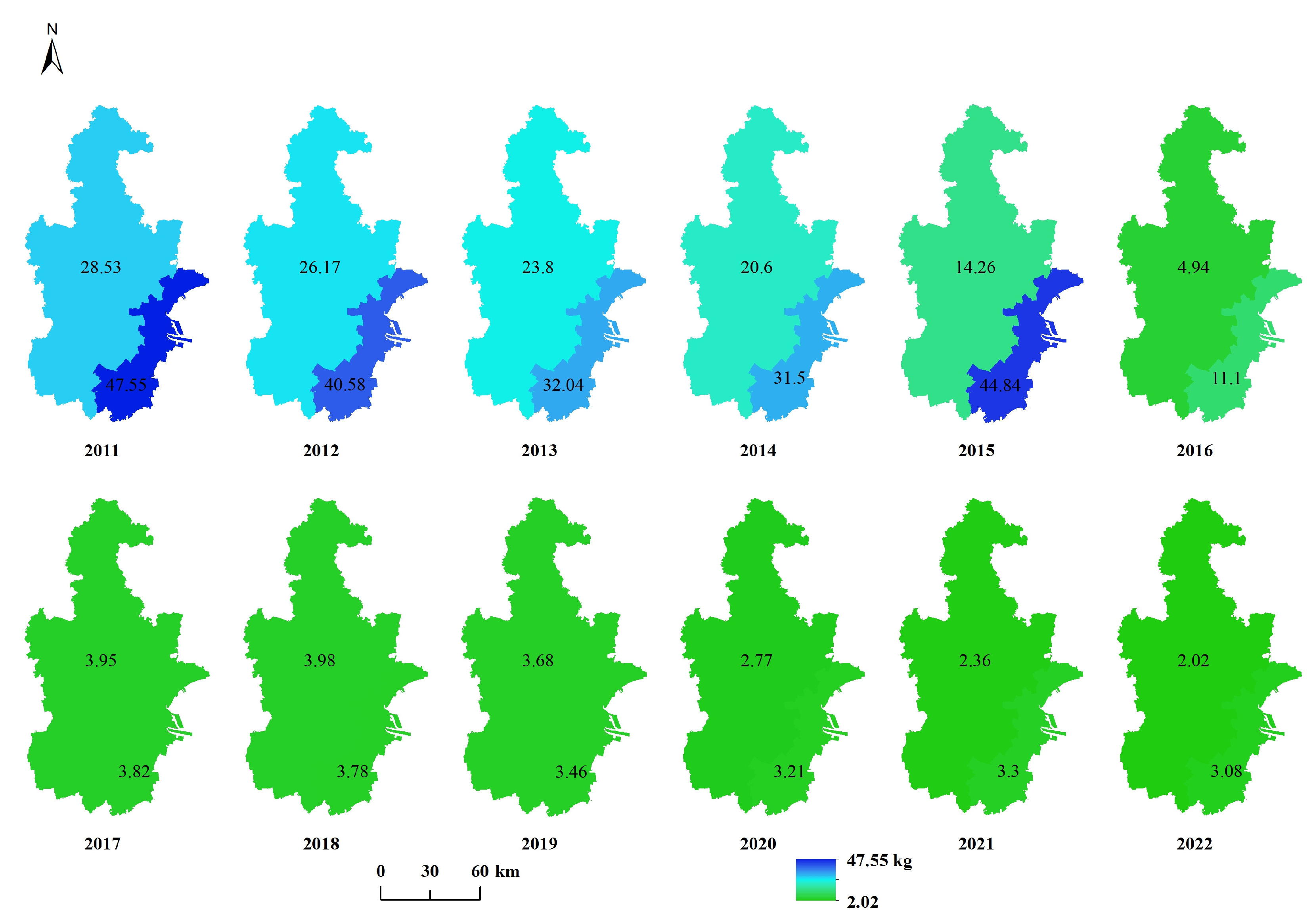
To better depict the spatiotemporal distribution of the statistical data used in calculating the EI score, the corresponding raster image is presented (Figure A1, Figure A2, Figure A3, Figure A4, Figure A5, Figure A6 and Figure A7). The label values in the figure represent the statistical values associated with each individual pixel. Based on data availability, the statistical units for COD, NH3, SO2, YFC, and NOX are divided into two regions: Tianjin and Binhai New Area. In contrast, the statistical units for WR and TAP encompass 11 distinct regions, including the Central Urban Area, Binhai New Area, Dongli District, Xiqing District, Jinnan District, Beichen District, Wuqing District, Baodi District, Jinghai District, Jizhou District, and Ninghe District.
Figure A1. Raster image of COD emissions from 2011 to 2022.
Land 14 01486 g0a1
Figure A2. Raster image of NH3 emissions from 2011 to 2022.
Land 14 01486 g0a2
Figure A3. Raster image of SO2 emissions from 2011 to 2022.
Land 14 01486 g0a3
Figure A4. Raster image of YFC emissions from 2011 to 2022.
Land 14 01486 g0a4
Figure A5. Raster image of NOX emissions from 2011 to 2022.
Land 14 01486 g0a5
Figure A6. Raster image of WR from 2011 to 2022.
Land 14 01486 g0a6
Figure A7. Raster image of TAP from 2011 to 2022.
Land 14 01486 g0a7

References

  1. Miao, C.-l.; Sun, L.-y.; Yang, L. The studies of ecological environmental quality assessment in Anhui Province based on ecological footprint. Ecol. Indic. 2016, 60, 879–883. [Google Scholar] [CrossRef]
  2. Yibo, Y.; Ziyuan, C.; Simayi, Z.; Haobo, Y.; Xiaodong, Y.; Shengtian, Y. Dynamic evaluation and prediction of the ecological environment quality of the urban agglomeration on the northern slope of Tianshan Mountains. Environ. Sci. Pollut. Res. 2023, 30, 25817–25835. [Google Scholar] [CrossRef] [PubMed]
  3. Liu, Q.; Qiao, J.; Li, M.; Dun, Y.; Zhu, X.; Ji, X. Spatiotemporal evolution of ecological environmental quality and its dynamic relationships with landscape pattern in the Zhengzhou Metropolitan Area: A perspective based on nonlinear effects and spatiotemporal heterogeneity. J. Clean. Prod. 2024, 480, 144102. [Google Scholar] [CrossRef]
  4. Wang, Y.; Wu, X.; He, S.; Niu, R. Eco-environmental assessment model of the mining area in Gongyi, China. Sci. Rep. 2021, 11, 17549. [Google Scholar] [CrossRef] [PubMed]
  5. Sun, L.; Yu, Y.; Gao, Y.; He, J.; Yu, X.; Malik, I.; Wistuba, M.; Yu, R. Remote Sensing Monitoring and Evaluation of the Temporal and Spatial Changes in the Eco-Environment of a Typical Arid Land of the Tarim Basin in Western China. Land 2021, 10, 868. [Google Scholar] [CrossRef]
  6. Zhu, D.; Chen, T.; Wang, Z.; Niu, R. Detecting ecological spatial-temporal changes by Remote Sensing Ecological Index with local adaptability. J. Environ. Manag. 2021, 299, 113655. [Google Scholar] [CrossRef] [PubMed]
  7. Boori, M.S.; Choudhary, K.; Paringer, R.; Kupriyanov, A. Eco-environmental quality assessment based on pressure-state-response framework by remote sensing and GIS. Remote Sens. Appl. Soc. Environ. 2021, 23, 100530. [Google Scholar] [CrossRef]
  8. Standard. Technical Criterion for Ecosystem Status Evaluation; China Environmental Science Press: Beijing, China, 2015. [Google Scholar]
  9. Wang, Q.; Gao, M.; Zhang, H. Agroecological Efficiency Evaluation Based on Multi-Source Remote Sensing Data in a Typical County of the Tibetan Plateau. Land 2022, 11, 561. [Google Scholar] [CrossRef]
  10. Wang, C.; Jiang, Q.O.; Shao, Y.; Sun, S.; Xiao, L.; Guo, J. Ecological environment assessment based on land use simulation: A case study in the Heihe River Basin. Sci. Total Environ. 2019, 697, 133928. [Google Scholar] [CrossRef] [PubMed]
  11. Clauset, A.; Larremore, D.B.; Sinatra, R. Data-driven predictions in the science of science. Science 2017, 355, 477–480. [Google Scholar] [CrossRef] [PubMed]
  12. Shumway, R.H.; Stoffer, D.S. ARIMA Models. In Time Series Analysis and Its Applications: With R Examples; Springer International Publishing: Cham, Switzerland, 2017; pp. 83–171. [Google Scholar]
  13. Ahmad, M.W.; Reynolds, J.; Rezgui, Y. Predictive modelling for solar thermal energy systems: A comparison of support vector regression, random forest, extra trees and regression trees. J. Clean. Prod. 2018, 203, 810–821. [Google Scholar] [CrossRef]
  14. Emmert-Streib, F.; Yang, Z.; Feng, H.; Tripathi, S.; Dehmer, M. An Introductory Review of Deep Learning for Prediction Models with Big Data. Front. Artif. Intell. 2020, 3. [Google Scholar] [CrossRef] [PubMed]
  15. Van Houdt, G.; Mosquera, C.; Nápoles, G. A review on the long short-term memory model. Artif. Intell. Rev. 2020, 53, 5929–5955. [Google Scholar] [CrossRef]
  16. Tong, X.; Feng, Y. A review of assessment methods for cellular automata models of land-use change and urban growth. Int. J. Geogr. Inf. Sci. 2020, 34, 866–898. [Google Scholar] [CrossRef]
  17. Liang, X.; Guan, Q.; Clarke, K.C.; Chen, G.; Guo, S.; Yao, Y. Mixed-cell cellular automata: A new approach for simulating the spatio-temporal dynamics of mixed land use structures. Landsc. Urban Plan. 2021, 205, 103960. [Google Scholar] [CrossRef]
  18. Zhou, Y.; Huang, C.; Wu, T.; Zhang, M. A novel spatio-temporal cellular automata model coupling partitioning with CNN-LSTM to urban land change simulation. Ecol. Model. 2023, 482, 110394. [Google Scholar] [CrossRef]
  19. Qin, W.; Ismail, M.H.; Ramli, M.F.; Deng, J.; Wu, N. Evaluation and Prediction of Ecological Quality Based on Remote Sensing Environmental Index and Cellular Automata-Markov. Sustainability 2025, 17, 3640. [Google Scholar] [CrossRef]
  20. Liang, L.; Song, Y.; Shao, Z.; Zheng, C.; Liu, X.; Li, Y. Exploring the causal relationships and pathways between ecological environmental quality and influencing Factors: A comprehensive analysis. Ecol. Indic. 2024, 165, 112192. [Google Scholar] [CrossRef]
  21. Chen, S.; Zhang, Q.; Chen, Y.; Zhou, H.; Xiang, Y.; Liu, Z.; Hou, Y. Vegetation Change and Eco-Environmental Quality Evaluation in the Loess Plateau of China from 2000 to 2020. Remote Sens. 2023, 15, 424. [Google Scholar] [CrossRef]
  22. Guo, Y.; Zhang, L.; He, Y.; Cao, S.; Li, H.; Ran, L.; Ding, Y.; Filonchyk, M. LSTM time series NDVI prediction method incorporating climate elements: A case study of Yellow River Basin, China. J. Hydrol. 2024, 629, 130518. [Google Scholar] [CrossRef]
  23. Zhang, T.; Yang, R.; Yang, Y.; Li, L.; Chen, L. Assessing the urban eco-environmental quality by the remote-sensing ecological index: Application to Tianjin, North China. ISPRS Int. J. Geo-Inf. 2021, 10, 475. [Google Scholar] [CrossRef]
  24. Han, H.; Guo, L.; Zhang, J.; Zhang, K.; Cui, N. Spatiotemporal analysis of the coordination of economic development, resource utilization, and environmental quality in the Beijing-Tianjin-Hebei urban agglomeration. Ecol. Indic. 2021, 127, 107724. [Google Scholar] [CrossRef]
  25. Yang, J.; Huang, X. 30 m annual land cover and its dynamics in China from 1990 to 2019. Earth Syst. Sci. Data Discuss. 2021, 2021, 1–29. [Google Scholar]
  26. Gao, J.; Shi, Y.; Zhang, H.; Chen, X.; Zhang, W.; Shen, W.; Xiao, T.; Zhang, Y. China Regional 250m Fractional Vegetation Cover Data Set (2000–2023); National Tibetan Plateau/Third Pole Environment Data Center: Beijing, China, 2024. [Google Scholar] [CrossRef]
  27. Yan, J.; Wang, S.; Feng, J.; He, H.; Wang, L.; Sun, Z.; Zheng, C. The 30 m Annual Soil Water Erosion Dataset in Chinese Mainland from 1990 to 2022; Science Data Bank: Beijing, China, 2024. [Google Scholar] [CrossRef]
  28. Abrams, M.; Yamaguchi, Y.; Crippen, R. ASTER GLOBAL DEM (GDEM) VERSION 3. ISPRS-Int. Arch. Photogramm. Remote Sens. Spat. Inf. Sci. 2022, XLIII-B4-2022, 593–598. [Google Scholar] [CrossRef]
  29. Peng, S. 1-km Monthly Mean Temperature Dataset for China (1901–2024); National Tibetan Plateau/Third Pole Environment Data Center: Beijing, China, 2024. [Google Scholar] [CrossRef]
  30. Peng, S. High-Spatial-Resolution Monthly Precipitation Dataset over China During 1901–2017; National Tibetan Plateau/Third Pole Environment Data Center: Beijing, China, 2019. [Google Scholar] [CrossRef]
  31. Peng, S. 1-km Monthly Potential Evapotranspiration Dataset for China (1901–2024); National Earth System Science Date Center: Beijing, China, 2024. [Google Scholar] [CrossRef]
  32. Mooney, P.; Minghini, M. A review of OpenStreetMap data. In Mapping and the Citizen Sensor; Ubiquity Press: London, UK, 2017; pp. 37–59. [Google Scholar]
  33. Lebakula, V.; Sims, K.; Reith, A.; Rose, A.; McKee, J.; Coleman, P.; Kaufman, J.; Urban, M.; Jochem, C.; Whitlock, C.; et al. LandScan Global 30 Arcsecond Annual Global Gridded Population Datasets from 2000 to 2022. Sci. Data 2025, 12, 495. [Google Scholar] [CrossRef] [PubMed]
  34. Alzubaidi, L.; Zhang, J.; Humaidi, A.J.; Al-Dujaili, A.; Duan, Y.; Al-Shamma, O.; Santamaría, J.; Fadhel, M.A.; Al-Amidie, M.; Farhan, L. Review of deep learning: Concepts, CNN architectures, challenges, applications, future directions. J. Big Data 2021, 8, 53. [Google Scholar] [CrossRef] [PubMed]
  35. Pang, B.; Nijkamp, E.; Wu, Y.N. Deep Learning with TensorFlow: A Review. J. Educ. Behav. Stat. 2020, 45, 227–248. [Google Scholar] [CrossRef]
  36. Whang, S.E.; Roh, Y.; Song, H.; Lee, J.-G. Data collection and quality challenges in deep learning: A data-centric ai perspective. VLDB J. 2023, 32, 791–813. [Google Scholar] [CrossRef]
  37. Ji, Z.; Wan, Y. A novel method for socioeconomic data spatialization. Spat. Stat. 2021, 43, 100501. [Google Scholar] [CrossRef]
  38. Ladosz, P.; Weng, L.; Kim, M.; Oh, H. Exploration in deep reinforcement learning: A survey. Inf. Fusion 2022, 85, 1–22. [Google Scholar] [CrossRef]
  39. Corso, G.; Stark, H.; Jegelka, S.; Jaakkola, T.; Barzilay, R. Graph neural networks. Nat. Rev. Methods Primers 2024, 4, 17. [Google Scholar] [CrossRef]
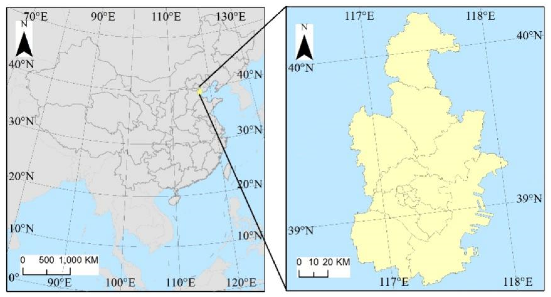
Figure 1. The location of the study area.
Land 14 01486 g001
Figure 2. Model framework for regional EEQ prediction and evaluation.
Land 14 01486 g002
Figure 3. Model framework for predicting statistical data using the ARIMA. R1 to Rn represent the statistical units of the statistical data.
Land 14 01486 g003
Figure 4. Model framework for conducting NDVI and SE prediction using a CNN-LSTM model.
Land 14 01486 g004
Figure 5. Model framework for conducting LUC prediction using a CA model coupled with both CNN and LSTM models.
Land 14 01486 g005
Figure 6. Spatiotemporal distribution of the absolute differences between the true and predicted EI values.
Land 14 01486 g006
Figure 7. Three typical examples of high EI errors based on multisource data integration.
Land 14 01486 g007
Table 1. Data and variables used in the study.
DataVariableDescription Resolution
LUCLUCLUC change data.30 m
NDVINDVIAnnual NDVI calculated as the average of maximum NDVI values from May to September.250 m
Soil erosionSESoil water erosion data in t/(hm2 a)30 m
ClimateTEM Annual mean temperature expressed with 0.1 °C units.1 km
PREAnnual mean precipitation in mm.1 km
PETAnnual mean potential evapotranspiration in mm.1 km
TopographyELEVElevation in m.30 m
ASPAspect in degrees.30 m
SLPSlope in degrees.30 m
TRITerrain ruggedness index in m.30 m
Spatial distance D2RWEuclidean distance from railway in m.-
D2RDEuclidean distance from road network in m.-
D2RVEuclidean distance from river network in m.-
PopulationPDPopulation density in terms of persons per pixel.1 km
Statistical dataCODCOD emission in ton.-
NH3Ammonia nitrogen emission in ton.-
SO2SO2 emission in ton.-
YFCSmoke (dust) emission in ton.-
NOXNitrogen oxide emission in ton.-
SOLSolid waste disposal in ton.-
WRWater resources in 100 million m3.-
TAPRegion’s total annual precipitation in mm.-
GDP/capitaPer capita GDP in CNY.-
Tertiary GDPGDP of the tertiary industry in 100 million CNY.-
EFEEducation financing expenditure in million CNY.-
STFEScientific and technological financing expenditure in million CNY.-
EPFEEnvironmental protection financing expenditure in million CNY.-
Table 2. EI values and subindex calculation formulas along with the utilized data.
IndexCalculation FormulaData Used
EI E I = 0.35 × H Q I + 0.25 × V C I + 0.15 × W D I + 0.15 × 100 L D I + 0.1 × ( 100 P L I ) -
HQI H Q I = A 1 × ( 0.35 × w o o d   l a n d + 0.21 × g r a s s l a n d + 0.28 × w a t e r   a r e a + 0.11   ×
    c r o p l a n d + 0.04 × c o n s t r u c t i o n   l a n d + 0.01 × u n u s e d   l a n d ) / r e g i o n   a r e a
LUC
VCI V C I = A 2 × ( i = 1 n P i ) / n NDVI
WDI W D I = ( A 3 × r i v e r   l e n g t h + A 4 × w a t e r   a r e a + A 5 × w a t e r   r e s o u r c e s ) / ( 3 × r e g i o n
a r e a )
LUC, Statistical data (WR)
LDI L D I =   A 6 × ( 0.4 × h e a v i l y   e r o d e d   a r e a + 0.2 × m o d e r a t e l y   e n o d e d   a r e a + 0.2   ×
c o n s t r u c t i o n   l a n d + 0.2 × o t h e r   l a n d   s t r e s s ) / r e g i o n   a r e a
LUC, SE
PLI P L I = 0.2 × A 7 × C O D   e m i s s i o n + 0.2 × A 8 × a m m o n i a   n i t r o g e n   e m i s s i o n / ( t o t a l  
a n n u a l   p r e c i p i t a t i o n ) + ( 0.2 × A 9 × S O 2   e m i s s i o n + 0.1 × A 10 × s m o k e   d u s t  
e m i s s i o n + 0.2 × A 11 × n i t r o g e n   o x i d e   e m i s s i o n + 0.2 × A 12 × s o l i d   w a s t e  
d i s p o s a l ) / r e g i o n   a r e a
Statistical data (COD, NH3, SO2, YFC, NOX
SOL, TAP)
Note: ① A1A12 refer to normalization coefficients; Pi is the mean of the monthly maxima of the NDVI from May–September; n is the number of pixels in the region. ② LUC classification differs from that of the EI model, as shrubland is classified as forestland in the HQI calculation. ③ The SOL in the study area is very small (less than 0.1 tons), so the solid waste disposal was set to 0 in the PLI calculation.
Table 3. Evaluation metrics for assessing the prediction results.
IndicatorCalculation MethodMeaning
RMSE R M S E = 1 m i = 1 m ( y i y ^ i ) 2 y i represents the actual value, y ^ i represents the predicted value, y ¯ i represents the mean of the actual values, and m represents the number of grids.Measures the average squared difference between the predicted and actual values. Smaller values indicate better accuracy, while larger values suggest higher errors.
MAE M A E = 1 m i = 1 m ( y i y ^ i ) Measures the average absolute difference between the predicted and actual values. Smaller values indicate higher accuracy, while larger values suggest more errors.
MAPE M A P E = 100 m i = 1 m ( y i y ^ i ) y i Measures the average absolute percentage difference between the predicted and actual values. Smaller values indicate higher accuracy, while larger values suggest greater errors.
R2 R 2 = 1 i = 1 m ( y i y ^ i ) 2 i = 1 m ( y i y ¯ i ) 2 Measures the fit between the predicted and actual values, ranging from 0 to 1. Values closer to 1 indicate better predictions, while values closer to 0 suggest poor degrees of fit.
OA O A = T P + T N T P + T N + F P + F N
TP denotes correctly transformed grids, TN represents correctly unchanged grids, FP signifies incorrectly transformed grids, and FN denotes incorrectly unchanged grids.
The proportion of correct predictions, with values closer to 1 indicating higher accuracy and values closer to 0 indicating lower performance.
Kappa K a p p a = p o p e 1 p e
P0 is the proportion of correctly predicted grids, while Pk represents the accuracy expected from performing random classification based on the grid distribution.
Measures accuracy by comparing the category distributions between the predicted and observed data, with values ranging from −1 to 1. Higher values indicate better accuracy.
Note: ① Due to the small sample size (only 10 data points from 2010 to 2019) in the ARIMA training, the R2 value is unreliable, and R2 is excluded from the evaluation of the statistical data prediction model. ② Since only one prediction value per year in the ARIMA, individual fluctuations may affect the stability of evaluation. Therefore, a multiyear assessment is used to improve the reliability of the results. ③ To ensure a more accurate assessment and avoid regional biases, the statistical data prediction model is evaluated by calculating the average prediction performance across different regions. ④ Because many values are zero, the MAPE is excluded from the SE prediction model evaluation.
Table 4. Statistical data prediction performance of the ARIMA model.
CODNH3SO2YFCNOXTAPWR
RMSE304.898.77945.14475.911662.92191.891.46
MAE269.814.02774.29422.721438.92137.871.03
MAPE17.6828.323.78.619.1815.933.68
Table 5. NDVI and SE prediction performance on the basis of the CNN-LSTM model.
YearNDVISE
RMSEMAEMAPER2RMSEMAER2
20200.050.0410.560.870.690.220.83
20210.060.0415.810.831.640.370.8
20220.070.0524.30.820.680.390.77
Table 6. LUC prediction performance on the basis of the CA-CNN-LSTM model.
YearKappaOA
20200.960.98
20210.960.97
20220.940.96
Table 7. EI score and EI level prediction performance.
YearEI ScoreEI Level
RMSEMAEMAPER2KappaOA
20202.081.393.230.970.850.91
20212.341.693.730.960.790.87
20222.641.944.290.960.760.85
Table 8. Total absolute errors of the EI score, its subindices, and the main contributing subindex counts in the study area.
Index202020212022
AE_ValueDI_CountAE_ValueDI_CountAE_ValueDI_Count
EI60,354.22/72,791.62/83,528.46/
HQI10,757.07146711,965.79135314,948.971875
VCI44,414.1322,49255,472.6423,36256,005.521,613
WDI15,128.86122736,231.2216,45427,194.24351
LDI6090.285103510,727.17168611,649.441811
PLI26,610.4116,6344946.03035,360.9713,205
Table 9. Total absolute errors of the EI score, its subindices, and the main contributing subindex count in regions with high EI errors (ΔE > 10).
Index202020212022
AE_ValueDI_CountAE_ValueDI_CountAE_ValueDI_Count
EI3532.11/3576.59/4564.23/
HQI2132.051642021.321552019.57145
VCI743.1831615.0221816.4928
WDI124.9702080231.050
LDI1020.31651132.61711880.84140
PLI91.37063.430233.760
Disclaimer/Publisher’s Note: The statements, opinions and data contained in all publications are solely those of the individual author(s) and contributor(s) and not of MDPI and/or the editor(s). MDPI and/or the editor(s) disclaim responsibility for any injury to people or property resulting from any ideas, methods, instructions or products referred to in the content.