Thermal Infrared UAV Applications for Spatially Explicit Wildlife Occupancy Modeling

Abstract

Assessing the impact of community-based conservation programs on wildlife biodiversity remains a significant challenge. This pilot study was designed to develop and demonstrate a scalable, spatially explicit workflow using thermal infrared (TIR) imagery and unmanned aerial vehicles (UAVs) for non-invasive biodiversity monitoring. Conducted in a 2-hectare grassland area in Chitwan, Nepal, the study applied TIR-based grid sampling and multi-species occupancy models with thin-plate splines to evaluate how species detection and richness might vary between (1) morning and evening UAV flights, and (2) the Chitwan National Park and Kumroj Community Forest. While the small sample area inherently limits ecological inference, the aim was to test and demonstrate data collection and modeling protocols that could be scaled to larger landscapes with sufficient replication, and not to produce generalizable ecological findings from a small dataset. The pilot study results revealed higher species detection during morning flights, which allowed us to refine our data collection. Additionally, models accounting for spatial autocorrelation using thin plate splines suggested that community-based conservation programs effectively balanced ecosystem service extraction with biodiversity conservation, maintaining richness levels comparable to the national park. Models without splines indicated significantly higher species richness within the national park. This study demonstrates the potential for spatially explicit methods for monitoring grassland mammals using TIR UAV as indicators of anthropogenic impacts and conservation effectiveness. Further data collection over larger spatial and temporal scales is essential to capture the occupancy more generally for species with larger home ranges, as well as any effects of rainfall, flooding, and seasonal variability on biodiversity in alluvial grasslands.

1. Introduction

In the face of escalating global environmental degradation, sustainable management initiatives are increasingly employing community-based conservation programs, including payments for ecosystem services (PES), to harmonize economic well-being with ecological sustainability. However, the reciprocal relationships between social systems and biodiversity outcomes in these programs remain understudied [1]. In particular, assessments of faunal biodiversity within PES initiatives often lack robust evaluations, limiting our understanding of any co-benefits to wildlife populations [2,3]. For instance, biodiversity restoration in PES areas may require intensive management strategies to meet the conservation goals [4]. Furthermore, the small size of many nature reserves underscores the need to evaluate conservation efforts in other areas where human and wildlife activities overlap.

In Nepal’s Terai lowlands, comprising riverine subtropical forests and alluvial grasslands, community-based conservation programs have emerged as critical tools for linking livelihoods with biodiversity conservation [5]. Across the Terai, significant losses of alluvial grassland habitat have occurred due to an increase in human pressure and conversion to other land use types, which has also led to a decline in the populations of many wildlife species [6,7,8,9]. Grassland ecosystems have historically supported local communities through activities such as livestock grazing, grass harvesting, and ecotourism. Initiatives like the Chitwan National Park Buffer Zone allow for regulated resource use while aiming to conserve biodiversity [10,11,12,13,14,15,16,17]. Government agencies and regional NGOs oversee the management of the grassland ecosystem, tourism infrastructure, and community-based conservation initiatives. However, the effects of such programs on wildlife populations remain inadequately quantified.

The Terai grasslands are renowned for hosting iconic large mammals such as the vulnerable greater one-horned rhinoceros (Rhinoceros unicornis), labeled as vulnerable by the International Union for the Conservation of Nature (IUCN), which has significantly increased in number [18], along with large carnivores such as the endangered tiger (Panthera tigris tigris) [19]. While governmental and NGO-led efforts have restored habitats and increased wildlife populations, understanding the spatial distribution of species under different management regimes is crucial for evaluating the success of conservation efforts. Specifically, spatially explicit data are critical for assessing the impact of community-based conservation on biodiversity.

Unmanned aerial vehicle (UAV) thermal infrared (TIR) imagery has shown promise as a cost-effective and efficient tool for wildlife surveys, with many studies investigating how to parameterize drone flights for the optimal capture of focal species [20,21,22,23,24,25,26], or which machine learning algorithms can best classify TIR imagery [27,28,29,30,31,32]. UAV TIR imagery can detect the heat signatures of animals, which, when combined with other identifying characteristics such as size, shape, and color, can help scientists identify different species [22,33]. This technology addresses the limitations of traditional methods, including ground-based surveys and camera traps, by offering accurate counts and scalability [34]. Despite its potential, UAV-based approaches face challenges in modeling UAV data, such as imperfect detectability and spatial autocorrelation, necessitating advanced statistical modeling techniques.

Like other types of population surveys, UAV TIR imaging poses its own set of unique sampling and analysis design challenges, such as imperfect survey detectability [35], resulting in numerous similar statistical modeling approaches being applied to TIR UAV imagery to address the detectability and sampling issues. These methods include hierarchical abundance modeling [36,37], N-mixture modeling [35,38], distance sampling [39], and logistic regression [40].

Occupancy monitoring aims to estimate the probability that a species occupies a site by collecting and analyzing data from a series of presence–absence surveys conducted at randomly selected sample sites within the study area [41]. Using data from repeated presence–absence surveys can alternatively be used to evaluate habitat use and occupancy [41,42,43], as demonstrated by the encouraging results of simulations [44] and field-based experiments [45]. Due to the ability of UAVs to repeatedly sample landscapes, particularly when systematically divided into a contiguous sampling of grid-based sampling blocks, one can detect species occurrences at a fine scale. Since grid-based sampling designs are not geographically independent, the geographic closure assumption may lead to biases, where the models represent “habitat suitability” rather than true “occupancy” [46,47]. Additionally, sampling with a grid-based sampling design introduces challenges to the reliability of statistical inferences. Methods have been developed to incorporate spatial terms that account for neighborhood locational effects and spatial autocorrelation [48,49,50,51,52]. The accuracy of species distribution models and mapping is improved by taking these factors into account during occupancy modeling, which reduces bias and increases the accuracy of occupancy estimates [53].

While the theoretical framework for occupancy modeling has become increasingly sophisticated—especially in accounting for spatial autocorrelation and sampling biases—the practical application of these methods using new technologies remains an emerging area of research. UAVs offer a promising tool for collecting fine-scale, repeatable presence–absence data, but their integration into spatially explicit occupancy models is still under development. In this context, we designed a pilot study to explore how UAV-based thermal infrared (TIR) imagery could support wildlife occupancy monitoring in complex, mixed-use landscapes. This pilot study utilized UAV-based TIR imagery to explore the feasibility of wildlife occupancy monitoring in Chitwan National Park and the adjacent Kumroj Buffer Zone Community Forest grasslands. Specifically, we aimed to: (1) compare mammal detectability between morning (5:30 a.m.–8:30 a.m.) and evening (5:30 p.m.–6:45 p.m.) UAV flights, (2) identify wildlife activity hotspots and patterns in species richness, and (3) demonstrate scalable analysis methods to assess the potential influence of park infrastructure and land management on wildlife activity. To meet these objectives, we conducted flights within a pre-defined 4.42-hectare grid to collect presence/absence data and applied Bayesian hierarchical spatially explicit multi-species occupancy modeling. The spatial footprint of our UAV survey was too limited to produce reliable or generalizable occupancy estimates for the focal species, whose home ranges far exceed the sampled area. Instead, the study was designed as a methodological pilot to test data collection and analysis workflows that could be scaled up with broader spatial coverage and additional replicates. Our findings provide proof-of-concept for the use of TIR UAV systems in monitoring large mammals in grassland ecosystems and offer insight into the optimal flight timing, modeling techniques, and potential applications for conservation planning. We discuss the advantages and limitations of using UAV TIR imagery for spatially explicit biodiversity assessment and highlight its potential in supporting community-based conservation programs and evaluating their effectiveness.

2. Materials and Methods

2.1. Study Area

Surveys were conducted in the Chitwan National Park (चितवन राष्ट्रिय निकुञ्ज) (27°33′24.1″ N 84°29′06.9″ E) and neighboring Kumroj Community Forest (कुमरोज कम्युनिटी फरेस्ट) (27°33′37.3″ N 84°30′23.2″ E) (Figure 1), within the Terai Arc Landscape (also known as the Terai Landscape or TAL). TAL is a network of terrestrial protected areas [8] featuring remnant alluvial grasslands and subtropical flora, ranging from early successional floodplain communities to climax Sal (Shorea robusta) forests [54]. These last remaining grasslands are managed as six protected areas in Nepal, where there is ongoing management for a matrix of “grazing lawns” and “tall grasses” to support high quality forage [55]. These ecosystems support diverse herbivore populations including rhinoceroses (Rhinoceros unicornis) and Asian elephants (Elephas maximus) as well as several ungulate species including gaur (Bos gaurus), sambar (Rusa unicolor), chital (Axis axis), barking deer (Muntiacus muntjak), hog deer (Axis porcinus), and wild boar (Sus scrofa). These ungulate species coexist with leopards (Panthera pardus fusca) and tigers (Panthera tigris tigris).

Chitwan NP, a UNESCO World Heritage Site established in 1973, spans 932 km² and includes a 750 km² buffer zone. The Buffer Zone is to the north of the park and protects natural resources and encourages ecotourism as managed by the Buffer Zone Act of 1993. This Act allows for the decentralization of forests that are located within the protected areas of the Terai [56]. The forest land immediately surrounding the Royal Chitwan National Park is subdivided into three distinct types of forest: state-owned forests, buffer zone forests, and buffer zone community forests (BZCF), the latter of which receives a portion of the park’s revenue to put toward environmentally responsible forest management [15].

Within this context, Kumroj Community Forest (established 1983) plays a significant role, with members actively gathering resources and generating income from tourism activities like safaris and boating. It has 2109 member households and generates NPR 3,000,000 annually (USD ~23,147). Its members have access to the grasslands every day to gather resources, primarily animal fodder, and are permitted to retrieve between three and five cubic feet (0.1 to 0.2 m³) of wood per year for construction purposes. Tourism accounts for 60–70% of the community forest’s income and consists primarily of jeep safaris, elephant rides, and boating. Tourists in safari jeeps travel along the dirt roads.

2.2. Data Collection

To evaluate species occupancy and habitat suitability, we conducted UAV surveys in Chitwan National Park (CNP) and Kumroj Community Forest (KCF) in Nepal. To evaluate species occupancy and habitat suitability, we used a series of steps to complete our evaluation (

Table 1. Steps used to evaluate species occupancy and habitat suitability including the study area delineation, UAV survey design, data processing, statistical modeling, and result visualization.

Task	Description
Study area overview	Delineate study areas in CNP and KCF.
Flight path design	Develop grid-based flight path overlays to ensure systematic area coverage.
Flight planning	Determine UAV flight parameters including altitude (77 m AGL), time of day (morning/evening), and camera configurations.
Data collection	Conduct UAV image capture using RGB and thermal cameras, with real-time detection at lower altitudes for species identification.
Data processing	Classify species manually from captured imagery and geolocate them.
Operability matrix generation	Generate a grid-based operability matrix indicating flown and non-flown cells using the UAV flight paths.
Presence/absence data collation	Aggregate species detection data into grid-based presence/absence datasets in ArcGIS pro.
Statistical modeling	Apply a multi-species occupancy model framework to the data in R.
Environmental covariates analysis	Analyze factors such as Euclidean distance to water and roads and block effects for land-use differences (KCF vs. CNP).
Spatial autocorrelation	Account for spatial autocorrelation using thin-plate splines to account for spatial dependencies.
Result processing	Estimate biodiversity metrics and conduct statistical comparisons using ANOVA.
Visualizations	Generate heatmaps and spatial maps to visualize species detection and biodiversity patterns.

).

UAV surveys were conducted using a DJI Mavic 2 Enterprise Advanced Drone (manufacturer: DJI, sourced: DSLR Pros San Diego, CA, USA) equipped with a 48-megapixel RGB camera and a 0.33-megapixel TIR camera. The thermal camera has a 16× zoom that can capture images at 30 Hz with a temperature measurement accuracy of 2 °C.

Thermal imaging was performed during morning (5:30–8:30 a.m.) and evening (5:30–6:45 p.m.) flights to maximize detection efficiency, as afternoon heat interfered with the thermal signatures (

Table 2. Dates of the flights flown in Chitwan National Park during the evening and morning for comparison.

P.M.	A.M.
25 May 2022	22 May 2022
21 May 2022	21 May 2022
8 May 2022	29 April 2022
7 May 2022	25 April 2022

). Flight parameters included a standard altitude of 77 m above ground level (AGL), yielding a swath width of approximately 90 m when the camera was oriented nadir. When tilted at a 45-degree angle, the swath expanded to approximately 278 m, which is the angle of view we used in this study. The thermal camera’s 16× zoom capability was utilized for species detection, complemented by lower-altitude flights when necessary to ensure accurate identification. If necessary, for finer-scale species identification, manual altitude adjustments were made as needed, typically lowering the UAV to a minimum of 30 m AGL to gain species ID.

Manual flight operations were used to fly each grid cell, requiring approximately six to seven batteries with a flight duration of 25 min each, plus five minutes for battery changes. The total imaging window typically lasted at least two hours and was equal between morning and evening flights. The same study gridded area was flown in entirety each time.

The second part of our study was based on UAV imaging flights within the Chitwan NP and Kumroj CF, with the purpose of comparing mammal composition between these two areas. Replicate flights were performed in both the CNP and KCF during mornings, based on findings indicating higher species detectability in cooler temperatures (

Table 3. Dates of the eight morning UAV imaging missions flown in Chitwan NP and Kumroj CF.

Chitwan NP	Kumroj CF
23 May 2022	28 May 2022
22 May 2022	27 May 2022
21 May 2022	26 May 2022
29 April 2022	24 May 2022

).

2.3. Data Processing

Species identification was performed entirely through manual visual inspection of the UAV-captured imagery. Animal detections were recorded in real-time during flights and subsequently verified through post-flight image analysis. Upon detection, UAV pilots adjusted the flight altitude or used the thermal camera’s zoom function to capture clear images for species identification.

2.4. Operability Matrix and Data Aggregation

Flight paths were processed in ESRI’s ArcGIS Pro (v. 3.4.0) to generate 150 m² grid cells, which facilitated the fine-scale assessment of spatial coverage across the study area. While the grid cell size was selected arbitrarily, it enabled consistent spatial referencing of the flight data. An operability matrix was constructed to indicate which grid cells were surveyed. A cell was classified as “flown” if the flight path intersected within 50 m of its center; otherwise, it was marked as “NA”. The final operability matrices marked 151 grid cells (2.26 ha) covering Chitwan NP, and 144 grid cells (2.16 ha) in Kumroj CF (Figure 2). A few grid cells along the edges may have initially not flown, so we accounted for them in the final analysis as an “NA” value for that survey.

Animal records were considered independent if they were at least five minutes apart from the last detection. These records were collated into grid cells using the image’s GPS centroid using a spatial join with the grid cell polygon. We aggregated these into daily presence/absence attributed datasets for each species separately.

2.5. Statistical Modeling

Hierarchical models refer to joint probability distributions that are broken down into a set of conditional distributions, enabling a modeler to break a large model into simpler segments [57]. Multi-species occupancy models (MSOMs) extend traditional single-species occupancy models to simultaneously estimate the occupancy of multiple species, accounting for imperfect detection [58,59,60]. Systematic surveys, though widely used, often vary in their design and equipment, which are rarely able to detect all species present at a site. The detectability of species can vary due to factors such as the technology used in survey equipment, the species’ body size, seasonal abundance, rarity, interspecific interactions (such as competition or predation), and environmental conditions like humidity and temperature [61]. To address these challenges, occupancy modeling uses detection and non-detection data to simulate a presence–absence framework, assuming that some species are not truly absent, but are simply imperfectly detected. The MSOM builds on this by incorporating multiple species, allowing for the estimation of species richness and community structure while considering imperfect detection [58]. The imperfect detection of species can be problematic, as undetected species may not be randomly absent—they could be locally rare, fulfill a unique ecological role, or represent distinct functional traits within the community [62].

In our study, we used a Bayesian hierarchical MSOM to estimate the community-level richness of medium to large terrestrial mammals across different forest reserves. The multi-region community model (MRCM) developed by [63] allows for the estimation of multi-species occupancy across geographically distinct regions, improving the statistical performance by incorporating random block effects. In our model, the observed data consisted of a site × sample matrix, where each cell represents a species’ detection (1) or non-detection (0) at a site during a survey.

The model structure is divided into two sections: one for the variance in occupancy between sites and another for the detection/non-detection data at the particular sites [64]. Multi-species occupancy models can include covariate information on both the occupancy ($\psi )$ and detectability ($p)$ aspects of the model, and they combine imperfect detection along with a model for species occurrence data (Equations (1) and (2)).

State process (occurrence):

$$z_{ik}~Bernoulli\left({\psi }_{ik}\right)$$

(1)

Observation process (detection):

$$y_{ijk}|z_{ik}~Bernoulli\left(z_{ik}{p}_{ijk}\right)$$

(2)

The models were replicated and parameterized at each site (i), survey replicate (j), and species (k) for both the occupancy ($\psi )$ and detectability ($p).$ The model presupposes independent parameters and prior distributions that are only somewhat informative. Detection probability is modeled as a function of both the z-matrix ($z_{ik})$(representing the site × species matrix) and the detection probability ($p)$ for each species at each site during a survey. Here, $y_{ijk}$ is the observed detection outcome, where $y_{ijk}$ = 1 if species k is detected at site i during survey j, and $y_{ijk}$ = 0 otherwise.

Environmental Covariates

Euclidean distances to roads and waterways were calculated using OpenStreetMap layers in ArcGIS Pro. We chose to use the Euclidean distance as it provides a straightforward and widely used method for calculating the spatial proximity. The map layer for roads included any dirt roads traversing the park, even those considered fire roads (which are rarely used in a fire emergency). Waterways were any riverine channel. We did not include small, artificially created watering holes. Rasters were downscaled to the predefined grid and then extracted at the centroid of a grid cell. The values were then centered and scaled prior to analysis.

Land use differences between the Kumroj Community Forest (Kumroj CF) and the Chitwan National Park (Chitwan NP) were added as a block effect (Chitwan NP vs. Kumroj CF). The Kumroj CF allows users to access the grasslands to collect fodder and other materials, whereas the National Park does not.

2.6. Spatially Explicit Multi-Species Occupancy Model Structure

Occupancy models assume a parametric structure. The parametric approach is flexible, where polynomials and various nonlinear functions of the covariates are parametric in nature, achieving well-fitted models [64,65]. Although very efficient, the parametric approach can be limiting for modeling new data and can be easily parameterized incorrectly. Therefore, non-parametric and semi-parametric approaches such as splines offer flexibility. Logistic and Poisson regressions can be fit with splines on one or all the predictors, which allows for the use of knots to fit the predictors at various lengths of the function. In the case of fitting a spatial spline as a covariate in the model, this can lead to better model fitting and more accurate spatial predictions (Equation (3)).

State process:

With thin-plate spline:

$$~{\beta }_0+\sum _{R=1}^R{b}_r{q}_{i,r}$$

(3)

At each spatial surface knot r, there is a beta (b_r) on the spline term. For the spline function, (b_r) is the set of penalized spline coefficients, and $q_{ir}$ is the (i,r)th entry of the design matrix $Q=Q_r{\Omega }_r^{1/2}$ corresponding to random effects in site occupancy [66]. The grid sizes of the analysis generated spatial knots. Knots and random effects were generated using AHMBook package functions in the R program [63].

All multi-species occupancy models included a thin-plate spline with covariates for distance to water and distance to roads (Equation (4)). To meet our second objective, we applied a block effect for land use in Chitwan NP and Kumroj CF (Equation (5))

$$~{\mathsf{\beta }}_0\left[k\right]+{\mathsf{\beta }}_2[k]\ast \mathrm{D}\mathrm{i}\mathrm{s}\mathrm{t} \mathrm{t}\mathrm{o} \mathrm{R}\mathrm{o}\mathrm{a}\mathrm{d}\mathrm{s}\left[i\right]+{\mathsf{\beta }}_3[k]\ast \mathrm{D}\mathrm{i}\mathrm{s}\mathrm{t} \mathrm{t}\mathrm{o} \mathrm{W}\mathrm{a}\mathrm{t}\mathrm{e}\mathrm{r}\left[i\right]+\sum _{R=1}^R{b}_r{q}_{i,r}$$

(4)

$$~{\mathsf{\beta }}_1\left[\mathrm{L}\mathrm{a}\mathrm{n}\mathrm{d}\mathrm{U}\mathrm{s}\mathrm{e}\left[i\right], k\right]+{\mathsf{\beta }}_2[k]\ast \mathrm{D}\mathrm{i}\mathrm{s}\mathrm{t} \mathrm{t}\mathrm{o} \mathrm{R}\mathrm{o}\mathrm{a}\mathrm{d}\mathrm{s}\left[i\right]+{\mathsf{\beta }}_3[k]\ast \mathrm{D}\mathrm{i}\mathrm{s}\mathrm{t} \mathrm{t}\mathrm{o} \mathrm{W}\mathrm{a}\mathrm{t}\mathrm{e}\mathrm{r}\left[i\right]+\sum _{R=1}^R{b}_r{q}_{i,r}$$

(5)

where (i) represents the site, and (k) represents the species in the multi-species model. The following vague priors for ${{\mathsf{\beta }}_0,\mathsf{\beta }}_2,{\mathsf{\beta }}_3$ were utilized: $\mu$ normally distributed (µ = 0, τ = 0.6), σ uniformly distributed (0, 10), and τ power transformed (σ, −2). In Equation (5), land use block covariate hyperparameters followed a normal distribution, denoted as ${\mathsf{\beta }}_1 ~Normal({\mu }_{{\beta }_r}, {\tau }_{{\beta }_r})$, where ${\mu }_{{\beta }_r}$ and ${\tau }_{{\beta }_r}$ respectively represent the mean and precision at the species level for each land use category (r).

Occupancy models can incorporate imperfect detection from any potential false absences during the survey [67,68]. The probability of detection ($p_{i,j,k}$) uses ${\alpha }_k$ to understand how these factors affect the species detectability (k) (Equation (6)). To meet the first objective of the study, we put a block effect on the AM or PM time signature of our surveys for each survey (j) and species (k) (Equation (7)). The observation process (detection) is represented as:

$$~{\alpha }_0[k]$$

(6)

$$~{\alpha }_0[AMPM[j],k]$$

(7)

Bayesian model fitting for all occupancy models was performed using the R program’s jagsUI package [69]. We ran three chains for 500,000 iterations while using non-informative priors, burning 250,000 and thinning 250. In order to evaluate the Bayesian p-values, a Bayesian posterior predictive check was performed [64]. Bayesian p-values were used to compare real data to hypothetical data, with p-values near 0.5 indicating a good fit (we considered anything ±0.05 of 0.5). The p-values were used to determine whether the data-generating process of the model could recreate the initial dataset [70].

2.7. Comparative Analysis of Species Richness and Beta Diversity Between Management Zones

To compare the species richness and Jaccard beta diversity between Chitwan NP and Kumroj CF, we conducted a one-way analysis of variance (ANOVA). In this study, ANOVA was used to test whether the differences in species richness and beta diversity metrics between Chitwan NP and Kumroj CF were significant. The analysis was conducted on both the complete Markov chain Monte Carlo (MCMC) outputs and the mean MCMC outputs for each model. The results were used to compare the effects of incorporating spline terms on detecting significant differences in diversity metrics.

3. Results

3.1. Temporal Variation in Species Occupancy and Richness

For the first objective, we evaluated whether morning (AM) and evening (PM) flights differed in species occupancy and species richness within Chitwan NP. The results revealed differences in the species occupancy and richness between morning (AM) and evening (PM) flights in Chitwan National Park’s grassland study area. In the raw grid counts, rhino and spotted deer were more frequently observed in the morning, and Asiatic black bear and wild boar were also spotted in the morning (

Table 4. Morning and evening grid counts of mammal species in the grassland study area of Chitwan National Park.

Species	A.M.	P.M.
Spotted deer	8	5
Sambar	0	4
Asiatic black bear	1	0
Tiger	0	1
Wild boar	1	0
Rhino	40	30
Hog deer	17	31
Gaur	3	2

). Hog deer were more frequently observed in the evening, and sambar and tiger were seen only in the evening. These findings highlight temporal variations in species presence across the two time periods.

Using multi-species occupancy models with covariates (distance to roads and water), with and without a spline term, and block effects for detectability, we found that the species detectability was generally higher during AM flights (

Table 5. (a) The results of the multi-species occupancy model, which included covariates (distance to roads and water), spline terms, and a block effect for detectability (morning vs. evening), were used to establish whether detectability was higher in the mornings or the evenings. The bold values indicate the higher values between the AM and PM surveys. (b) The results of the multi-species occupancy model, which included covariates (distance to roads and water) and a block effect for detectability (morning vs. evening), were used to establish whether detectability was higher in the mornings or the evenings. This model included no spline terms. The bold values indicate higher values between the AM and PM surveys.

(a)
Model	Variable	Rhino	Hog Deer	Spotted Deer	Asiatic Black Bear	Wild Boar	Sambar	Elephant	Gaur	Tiger
Detectability	AM	0.137	0.143	0.060	0.008	0.008	0.012	0.016	0.013	0.003
	PM	0.103	0.020	0.007	0.003	0.008	0.010	0.007	0.015	0.007
Occupancy (Psi)	Intercept	28.3	23.8	6.2	0.29	−0.18	3.0	0.69	3.1	0.72
	Roads	0.69	−0.90	−0.83	−0.27	−0.07	0.22	−0.08	0.51	−0.69
	Water	0.51	0.22	0.01	0.19	0.21	0.21	−0.15	0.29	0.28
	Occupancy (Psi)	0.79	0.75	0.56	0.53	0.44	0.56	0.51	0.53	0.56
(b)
Model	Variable	Rhino	Hog Deer	Spotted Deer	Asiatic Black Bear	Wild Boar	Sambar	Elephant	Gaur	Tiger
Detectability	AM	0.113	0.123	0.051	0.054	0.021	0.018	0.023	0.017	0.023
	PM	0.086	0.017	0.006	0.014	0.016	0.014	0.009	0.018	0.050
Occupancy (Psi)	Intercept	6.87	5.94	3.01	−1.24	2.25	4.08	3.83	4.60	−2.17
	Roads	−0.82	−2.46	−2.73	−1.93	0.63	−0.65	0.19	−0.30	−2.16
	Water	−0.30	0.28	0.28	0.63	−0.10	0.63	−0.46	−0.06	0.87
	Occupancy (Psi)	0.95	0.90	0.72	0.33	0.56	0.72	0.70	0.75	0.30

a,b). We also generated a series of hotspot maps for each species and the species richness for both models (Appendix A), highlighting spatial patterns of occupancy and demonstrating the application of the spline technique for hotspot mapping using the UAV data.

3.2. Spatial Variation in Species Occupancy and Richness Between Management Zones

For the second objective, we compared the species occupancy and richness between Chitwan NP and Kumroj CF. The results of the surveys revealed wildlife detections of seven species (one-horned rhinoceros, chital, sambar deer, hog deer, Asiatic black bear, gaur, and wild boar). There were more grid cell counts of spotted deer, wild boar, and hog deer observed in Kumroj CF (

Table 6. During four grid flights in each zone, seven species of large mammals were collated to the predefined grid in the grassland study areas of Chitwan NP and Kumroj CF.

Species	Chitwan NP	Kumroj CF
Spotted deer	10	24
Sambar	2	1
Asiatic black bear	2	0
Wild boar	2	10
Rhino	18	14
Hog deer	26	53
Gaur	1	3

).

We were able to generate multi-species occupancy models with covariates, block effects on land use (Chitwan NP or Kumroj CF) with no detectability covariates, with and without spline terms (

Table 7. (a) The results of the multi-species occupancy model, which included covariates (distance to roads and water), spline terms, and a block effect for land use (Chitwan NP vs. Kumroj CF) with no detectability covariates, were used to establish whether there was a significant difference between Chitwan NP vs. Kumroj CF. The bold values indicate the higher values between Chitwan NP vs. Kumroj CF. (b) The results of the multi-species occupancy model, which included covariates (distance to roads and water) and a block effect for land use (Chitwan NP vs. Kumroj CF) with no spline terms and no detectability covariates, were used to establish whether there was a significant difference between Chitwan NP vs. Kumroj CF. The bold values indicate the higher values between Chitwan NP vs. Kumroj CF.

(a)
Model	Variable	Hog Deer	Spotted Deer	Rhino	Wild Boar	Sambar	Asiatic Black Bear	Gaur
Detectability		0.075	0.059	0.054	0.021	0.015	0.010	0.015
Occupancy (Psi)	Chitwan NP land use	6.09	4.90	7.56	1.77	4.12	4.58	3.20
	Kumroj CF land use	7.95	5.51	2.25	7.56	−3.07	1.31	−7.41
	Roads	0.53	1.13	1.48	0.62	−0.02	−0.05	0.05
	Water	0.26	0.28	0.34	0.09	3.33	0.10	−1.46
	Occupancy (Psi)	0.96	0.86	0.83	0.77	0.49	0.66	0.41
(b)
Model	Variable	Hog Deer	Spotted Deer	Rhino	Wild Boar	Sambar	Asiatic Black Bear	Gaur
Detectability		0.09	0.10	0.07	0.03	0.02	0.01	0.01
Occupancy (Psi)	Chitwan NP land use	2.97	−0.45	3.84	0.54	−0.06	−0.08	0.46
	Kumroj CF land use	3.47	−0.69	3.16	0.74	0.16	0.05	−0.05
	Roads	0.23	−0.61	1.65	−0.14	−0.27	0.06	0.28
	Water	2.48	0.25	3.47	0.45	0.73	0.18	0.00
	Occupancy (Psi)	0.70	0.41	0.57	0.56	0.42	0.54	0.56

a,b). The model with the spline terms showed that rhino, sambar, Asiatic black bear, and gaur generally preferred the Chitwan NP, and that hog deer, spotted deer, and wild boar generally preferred Kumroj CF. The model without the spline terms showed that spotted deer, rhino, and gaur preferred the Chitwan NP, and that hog deer, wild boar, sambar, and Asiatic black bear preferred Kumroj CF.

3.3. Differences in Species Richness and Beta Diversity Between Zones

For spline-based models, the species richness differed significantly across all MCMC outputs but not in mean outputs (

Table 8. Results from the one-way ANOVA showing the significant differences between land use for species richness and Jaccard beta diversity. The results include the test run on all MCMC outputs and only the mean outputs.

	Covariates		Covariates Plus Spline
	Land Use All MCMC	Land Use Mean MCMC	Land Use All MCMC	Land Use Mean MCMC
Species richness	<2 × 10−16	<2 × 10−16	<2 × 10−16	0.155
Jaccard	0.285	N/A	<2 × 10−16	N/A

). In contrast, the non-spline models showed significant differences in both cases, with Chitwan NP exhibiting higher mammalian diversity overall. Beta diversity was significantly greater within Chitwan NP in the spline-based models, whereas the non-spline models found no such difference.

3.4. Visualization of Hotspots of Species Occupancy and Richness Patterns

We developed hotspot maps for individual species and species richness for both model configurations (Appendix A). These visualizations underscore areas of high occupancy and highlight key differences in species distribution across temporal and spatial scales.

4. Discussion

This study employed a spatially explicit multi-species occupancy modeling approach using TIR UAV imagery as a pilot effort to test the feasibility of using TIR flight collected data in monitoring spatial patterns of biodiversity. Rather than drawing broad ecological conclusions, the study was specifically designed to evaluate data collection workflows, modeling techniques, and flight timing protocols that can inform future large-scale biodiversity assessments. Our findings offer initial insights into mammal occupancy dynamics across temporal windows and land management zones in a mixed-use conservation landscape. In regions where human–wildlife coexistence is both vital and complex, the development of scalable, non-invasive monitoring workflows are essential for effective biodiversity conservation and adaptive management.

4.1. Temporal and Spatial Patterns of Occupancy

The results attempted to determine temporal variation in mammal occupancy, with slightly higher detection probabilities in the morning compared with the evening. Consequently, subsequent flights for zonal comparisons were conducted during morning hours.

Spatially, our pilot study findings indicate comparable biodiversity levels between Chitwan NP and Kumroj CF, as determined by the model with the thin-plate spline, which accounts for spatial autocorrelation. This suggests that the workflow for data analysis could be suitable for larger surveys with more spatial and temporal replicates for assessing the effectiveness of community-based conservation programs in maintaining biodiversity while supporting ecosystem service extractions. Chitwan NP, established in 1973, and Kumroj CF, established in 1983, represent areas with different human impact and resource use. Despite permitting the daily extraction of animal fodder, firewood, and timber by 2109 households, Kumroj CF supported comparable ungulate populations to the Chitwan NP in our model results. Our TIR UAV surveys indicate a higher daily raw count of several mammals, including spotted deer, hog deer, and wild boar, within grid cells in the Kumroj CF, indicating that the count of ungulate mammals is comparable or even higher to the areas directly within the national park for several species. These results highlight the potential of community-based conservation in meeting aspects of conservation goals alongside sustainable resource use. However, longer-term studies involving several flights per month over a few years would provide additional, comprehensive evidence to support the results from this small pilot study dataset.

4.2. Estimating Detection Probabilities from UAV Flights

Detection errors in UAV surveys can bias abundance estimates if not addressed. These errors include false negatives (availability and perception errors) and false positives (misidentification and double counts), which vary based on the species traits, site conditions, and survey design [36,71]. Hierarchical models provide an integrative framework for addressing detection errors, combining multiple datasets, and accounting for observer and environmental variation [36].

Each flight was treated as an independent sampling event, constructing detection histories for each species to estimate the detection probabilities while accounting for imperfect detection. Species detectability across the study area was generally low (<0.20), underscoring the need for increased sampling frequency and additional flights for a more robust survey. Detectability was generally higher in the morning (AM) for most species across both models (with and without spline terms). Notably, rhinoceros, hog deer, and spotted deer exhibited higher morning detectability values. Low detection probabilities pose challenges for long-term population monitoring, including insufficient power to detect a 20% population decline over time, rendering surveys less effective [72]. Larger scale sampling efforts beyond this pilot study would be useful for qualifying these models and improving the accuracy of detectability estimates.

4.3. Advantages of UAV TIR and RGB Cameras for Wildlife Monitoring

The TIR camera was primarily used to detect the heat signatures of animals, which is particularly advantageous for identifying cryptic or nocturnal species that are challenging to observe with visible light cameras or camera traps. These methods have been found to have a higher detection probability compared with RGB cameras for detecting humans [29] and kangaroos [20]. The RGB camera complemented the TIR imagery by providing high-resolution visuals for species identification during the morning or evening hours, similar to other studies [73]. This dual-camera approach leverages the strengths of both technologies, with the TIR camera excelling in initial detection and the RGB camera ensuring accurate species classification.

Drones equipped with TIR and RGB cameras offer unique advantages for wildlife monitoring compared to traditional methods, such as camera traps or direct observation [20,26,74]. Due to the challenges of detectability and surveying an entire grid cell, occupancy models have biases related to non-detection errors when the species is present in the survey method [75]. While these methods also encounter detectability issues, TIR-based surveys can comprehensively sample entire grid cells, potentially providing better species trend detection. Simulation studies suggest that camera trapping has limited power for trend detection due to the small effective area sampled within grid cells, emphasizing the need for careful consideration of field efforts and the effective area of sampling devices [72]. Since the TIR UAV method samples the entire effective area of a grid cell, we suggest that TIR UAV grid sampling provides a spatially more comprehensive sampling coverage, although it is temporally limited to the flight time. Previous simulation studies on grid-based sampling support this designs that varied the home range and effective area sampled within grid cells, concluding that camera trapping has low power to detect trends due to the relatively small effective area sampled within the grid cell by the camera [72]. TIR UAV methodologies may be used alongside or integrated with camera trapping data to assess the sampling efficacy and identify long-term trends [45].

It is important to note, however, that the Nepal Terai grasslands provided an ideal test environment for UAV-based thermal surveys. The open, flat terrain and minimal canopy cover allowed for clear visibility and heat signal detection from above, increasing the likelihood of accurately spotting wildlife. In more complex landscapes—such as forested, mountainous, or densely vegetated environments—the effectiveness of TIR detection may be reduced due to obstruction of thermal signatures by vegetation or terrain, and thus may require methodological adjustments.

4.4. Survey Design and Spatial Resolution Considerations

The limited size of the study area is acknowledged, and a more extensive survey design is recommended to assess the species distribution under human pressure. Flight paths were processed in ArcGIS to generate 150 m² grid cells, facilitating fine-scale spatial assessment across the study area. Although this grid-cell size was selected somewhat arbitrarily, it enabled consistent spatial referencing of flight data and precise identification of areas covered or missed during each UAV survey. Notably, the UAV’s swath width of 278 m ensured comprehensive coverage of these 150 m² grid cells along the flight paths, allowing us to fly comprehensively using these finer-scale blocks to ensure complete coverage of the study area and minimize spatial gaps.

This fine-scale resolution also provides a flexible framework for scaling and aggregation. Depending on the study objectives—whether to detect localized activity patterns, monitor broader occupancy trends, or integrate with coarser-resolution datasets—the 150 m² grid cells can be aggregated into larger units or standardized to match other spatial scales. For example, if the study area consists of fifteen separate 2-hectare units, the fine-scale grid cells within each unit can be combined to summarize wildlife activity or occupancy at the broader scale. Such aggregation reduces noise from small-scale variation and improves interpretability for landscape-level planning.

Although previous studies have noted that UAVs are especially promising in smaller, community-managed wildlife areas where they can supplement traditional methods and provide real-time, high-quality ecological data [76], expanding the study to additional grassland-based community forest programs in Nepal and India would allow for comparisons with national park programs. Increasing the survey visits and replicates of sampling blocks would be more practical for capturing the habitat use of large ranging mammals for improving detectability and understanding long-term species trends. Given the pilot study’s eight-flight dataset, seasonal effects are likely, necessitating weekly or biweekly flights over a year to assess detectability across seasons and environmental variability, such as rainfall, and conduct power analyses.

4.5. Spatial and Ecological Drivers of Species Occupancy

4.5.1. Patterns of Occupancy and Preliminary Inferences

Rather than aiming for broad ecological inference, our primary objective was to evaluate the feasibility and limitations of modeling TIR UAV data with fine-scale covariates. We caution against interpreting the results of zone-level differences as solely the result of management regimes; instead, we present these patterns as preliminary findings that serve as a template for future research. These results warrant further investigation with expanded spatial and temporal replication appropriate to the home ranges of large mammals. While the limited size of our study area precluded consistent or generalizable conclusions, the analysis provides a foundational framework for data processing and highlights the potential of TIR UAV methods for multi-species multi-region occupancy modeling.

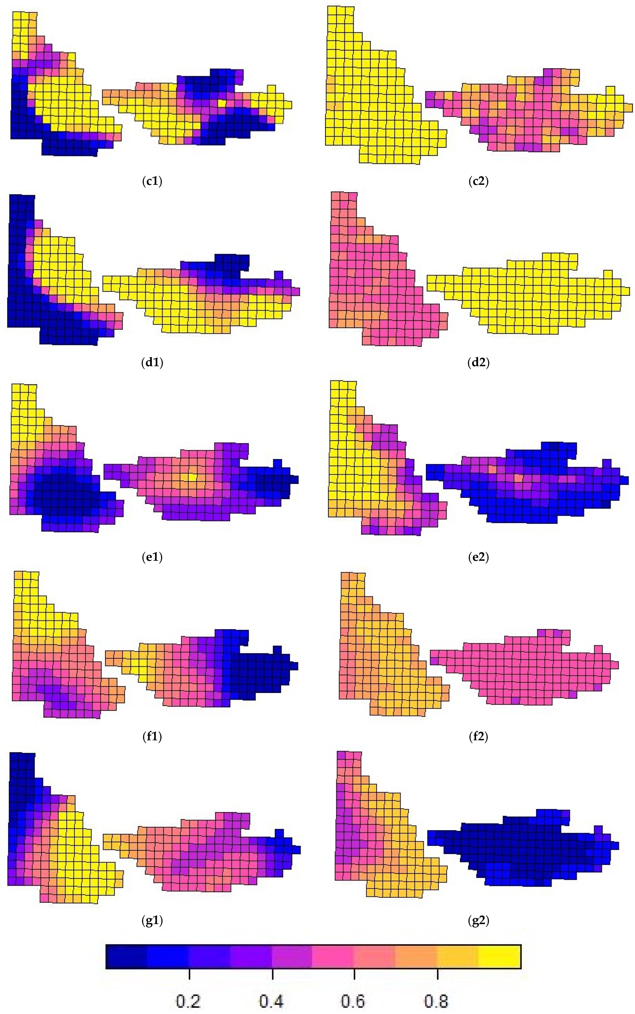
Despite any variations in covariate effects, habitat use “occupancy” estimates across the study area were generally high (>0.40 psi), with hotspot maps highlighting species-specific spatial preferences. Chitwan NP exhibited higher occupancy estimates for rhinoceros (7.56), sambar (4.12), Asiatic black bear (4.58), and gaur (3.20), indicating that these species may prefer the protected and undisturbed habitats of the national park. Conversely, Kumroj CF had a higher occupancy for hog deer (7.95), spotted deer (5.51), and wild boar (7.56), suggesting that these species may thrive in community-managed environments with habitat heterogeneity or human intervention. However, additional data replicates are needed to confirm these patterns, along with finer-scale information on human activity within each zone. The two sites—Chitwan National Park and Kumroj Community Forest—are separated by the Rapti River, which acts as a partial movement barrier for many terrestrial species, particularly during the monsoon. However, we acknowledge that it is not an impermeable boundary for all wildlife, especially wide-ranging species such as elephants or tigers. Additionally, access is regulated and limited for community use in the Community Forest, and some tourist-related hiking is permitted in the National Park, where some areas experience more intensive human use than others. These considerations became more apparent as the study progressed and should be considered for future studies investigating fine-scale impacts in community conservation areas.

Environmental covariates also influenced the species distribution patterns, but their effects varied between the first (AM/PM) and second surveys (Chitwan/Kumroj). This suggests that additional data would improve our understanding of these covariate effects.

4.5.2. Habitat Preferences, Disturbance, and Future Considerations

Previous research in Chitwan has highlighted correlations between various animal species and habitat types, despite many large mammals being generalists [11]. Human disturbance has been shown to negatively affect tiger prey species [11], and although primates and muntjac displayed a preference for highly disturbed areas, they generally favored less disturbed locations, even when the habitat quality was higher in more impacted areas. Similar studies have shown that leopards avoid roads and deforestation [54]. Predator rich areas were avoided by a few species [11], highlighting the interspecific effects not captured in our analysis. The study emphasizes that conservation priorities should focus on minimizing human impact and restoring buffer zone forests to protect the park ecosystem [11].

Since many of the large mammal species detected in the study area are foraging herbivores, future studies may seek to identify gradients of landscape variability within grassland environments (e.g., quantifying finer-scale grassland vegetation types may enhance the study and provide more information about the landscape’s diversity). Similarly, edge effects from adjacent forest areas may also provide an important factor for inclusion in future studies. Previous studies have shown that various factors, such as grass height, community composition, flood history, and fire history, are fine-scale habitat use factors [77]. Furthermore, many of the species in our study area exhibit seasonal food habits, which are influenced by seasonal forages, and this will also impact their distribution on the landscape [78]. However, there can be large variability in covariate response for different species between years, prompting longer term studies for robust estimates of covariate response [79]. Like our research, a study on large herbivores in China used UAV surveys with an RGB camera, flying large sample areas of varying sizes to sample several management zones to identify and discuss the effects of grazing pressure on livestock and wild herbivores [80]. These methods will prove useful in identifying the optimal foraging habitats or in determining whether restored or managed habitats are being used by the herbivore species.

4.6. Methodological Contributions

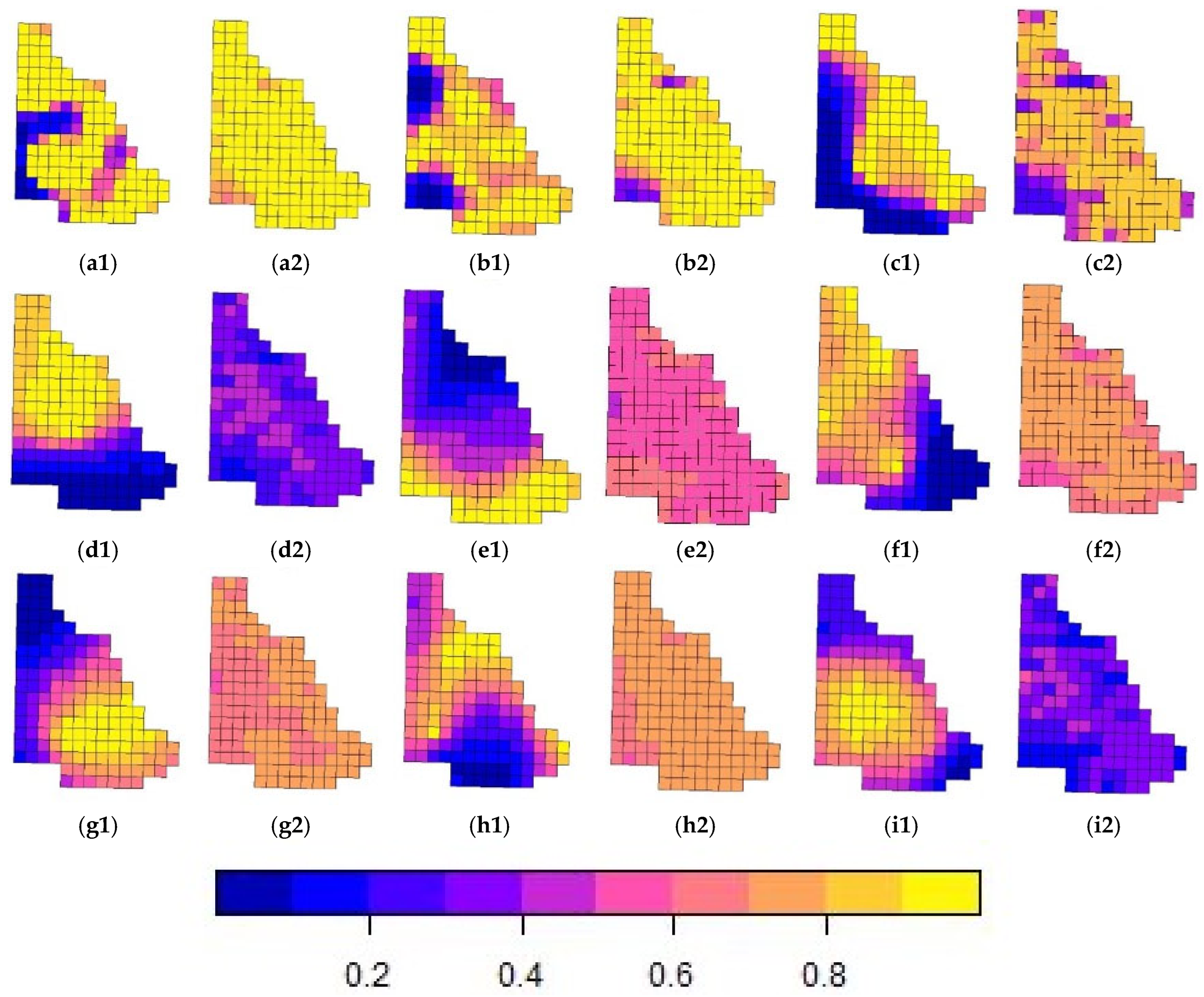
This study is the first to integrate spatial thin-plate spline terms into TIR UAV-based occupancy models, providing a refined method for visualizing habitat suitability and identifying biodiversity hotspots. Accounting for autocorrelation highlights fine-scale differences among samples compared with standard occupancy models, which often overlook the interdependence between grid cells. This approach allowed us to test covariate sets, including ecological and anthropogenic variables, while accounting for spatial autocorrelation. Models with and without spatial spline terms offered varying results: the spline-inclusive model showed no significant difference in species richness between the two zones, while the model without splines identified significantly higher richness in Chitwan NP (Figure 3, Table 7). Additionally, beta diversity differences between the zones were significant in the spline-based model, emphasizing the importance of addressing spatial autocorrelation in ecological analyses (Figure 3, Table 7). Since our results were from a pilot study, more data collected over longer periods within different seasons are required to further qualify these results. This study serves as a demonstration of the techniques and application of the models.

Numerous studies have demonstrated the efficiency of TIR UAV surveys for gathering information on the occurrence of various species [74,81,82,83], although few have attempted to apply species distribution models to these data. In occupancy modeling, spatial autocorrelation is most commonly addressed by incorporating autologistic terms, which account for the presence of a species in neighboring grid cells through a spatial weight matrix [53,84,85]. More recently, spatial autocorrelation has been addressed using basis functions (i.e., splines) to understand complex nonlinearities in spatiotemporal ecological relationships [50]. Semiparametric modeling approaches, such as generalized additive models (GAM), use thin-plate splines to produce a basis expansion on the distances between spatial grid cells and knots placed over the study area to produce a smoothing matrix, similar to a GAM smooth, which can account for the random effects of spatial autocorrelation between locations [50,63,86,87]. The application of splines in ecological research is applied widely on covariates and placement within models. In this way, the shape of the functional relationship between the response and predictors is data driven, whereas in a parametric model, the shape is determined by the model specification itself [88]. While previous studies have demonstrated the utility of splines for smoothing spatial trends, their application to UAV-derived occupancy data at such a fine scale remains underexplored.

Due to the diversity of wildlife in the landscape, the spline terms generated an extensive range of habitat suitability estimates within the predefined grid, with some grid cells having probabilities close to the highest value 1 and others having the lowest likelihood. Since the covariates in our study did not determine significant effects that influenced the model estimates, the spline terms allowed for a finer-scale hotspot distribution map to be generated based on the grid as well as for any issues with spatial autocorrelation to be resolved.

One prior study using long-term data collected from manned pilot aerial surveys covering the entire county of Lampikia in southern Kenya used Bayesian hierarchical multi-species modeling with three covariates and applied a smoothing spline for visualizing trends [89]. Their study found that wildlife-friendly properties support more diverse animal populations than other land uses. In contrast, pastoral lands had the lowest herbivore species richness, largely due to the wild herbivores’ negative response to cattle. An occupancy model was used in another manned piloted study on wolverine tracks in Alaska to model a hexagonal grid with four spatially explicit covariates without using a spline parameter [90]. These manned aerial flights were able to cover a larger area than the UAV in our study could fly, thus increasing the amount of land covered in comparison to our own study. Other studies have attempted a spatially explicit grid sampling approach with random site selection that was used to collect samples of dugongs using a UAV equipped with an RGB camera [81]. Dugong data were used to generate a density surface model that employed a generalized additive model, which makes use of a smooth spline term selected through restricted maximum likelihood (REML), to create dugong hotspot maps of the region. Along an environmental gradient, an experiment involving UAV and a tennis ball experimental design was conducted to determine how well occupancy models and auto-logistic occupancy could model the distribution of tennis balls, showing potential for environmental studies [45]. Here, we incorporated a spatial spline term into the occupancy models and found it useful for the purpose of visual comparisons using plotted maps, which depicted clustered areas on the landscape.

The choice of modeling approach, multi-species occupancy, and MSOM could benefit from also utilizing multivariate approaches such as a redundancy analysis (RDA) [79,91]. The RDA uses similar multi-species data matrices, although there is no hierarchical modeling component for imperfect detection. For a larger scale study, the use of RDA may also qualify the block effects between the national park and community forest, being a significant source of variation [91]. RDA models do not consider the effects of detectability, although they can use multi-species data to evaluate the covariate effects based on the raw count matrices and determine what percentage of the variation in the data can be described by the various covariates more generally [79,91].

4.7. Study Design Considerations for TIR Drone in Wildlife Monitoring

In a primer on flight methods (Bohnett, in review), the effectiveness of manually flying a pre-defined grid was compared with a programmed, automated flight routine. The study found no significant differences in mammal detection between the two approaches; however, manual flights were notably shorter and required fewer post-processing steps. Both methods exhibited observational biases, with programmed flights involving extensive post-flight processing and challenges related to manual observer errors and species identification. Based on these findings, the study recommended a hybrid approach, similar to the method adopted in the present research, to enhance replicability. Previous studies have also employed video-based, double-observer strategies for virtual transects to achieve comprehensive species identification [20].

4.7.1. Optimizing UAV Survey Design

Additional research has explored UAV flight plan optimization for wildlife surveys. One study used a grid-based simulation model to examine detection errors under different flight configurations, including variations in altitude and speed [44]. Their study demonstrated a method where linear transects were sampled within the grid, and they generated four contrasting flight options as combinations of flying at high or low altitude, and at fast or slow speed. They found that low and slow flights consistently provided the best estimates of abundance and occupancy, but higher or faster flights resulted in more complex guidelines for estimates of abundance or occupancy over larger study areas. These sampling designs differed from our strategy of systematically sampling the entire grid, although future studies may consider alternative sampling schemes. Some studies have also employed random block sampling from predefined grids [81,92], a strategy partially mirrored in this research, which employed two large blocks sampled extensively at a finer grid scale. Future research could benefit from incorporating additional sampling blocks to increase the survey coverage and robustness.

4.7.2. Wildlife Disturbance and Ethical Considerations

While TIR UAVs offer a non-invasive and efficient means of monitoring wildlife, their potential impact on animal behavior and stress must be considered. Even though most of the study animals did not respond behaviorally to the UAS flying at 80 m AGL and behavioral responses to UAVs were minimal in this study, physiological stress effects remain an area of concern. Addressing these impacts is critical for developing ethical and effective monitoring protocols. Wildlife disturbance must be taken into account by UASs because it may reduce the fitness and survival of certain animal species [93]. The heart rates of American black bears were monitored with biologgers to assess a reaction to UAS flights, showing an increase in heart beats per minute, even if they are not moving or reacting physically, and that they also habituate to the sound of the aircraft over time [94,95]. Other species, like the guanaco, have been studied observationally, showing that the guanaco reacted at lower heights (60 m above ground level AGL) and had less reactivity at higher heights (180 m AGL) and lower speeds (2–4 m s) [96]. A study in Botswana using two UAVs to observe seven herbivore species in the Moremi Game Reserve found that flights below 60 m AGL or within 100 m of animals triggered behavioral responses, particularly in elephants, giraffes, wildebeests, and zebras, highlighting the need for regulations to minimize wildlife disturbances [97]. Certain animals have been shown to be more sensitive than others, where potential impacts can be assessed in the field prior to any long-term monitoring program.

4.8. Managing Human–Wildlife Conflicts in Shared Landscapes

The coexistence of large mammals and humans in shared landscapes necessitates proactive management to mitigate conflicts and support conservation goals. The long-term monitoring of wildlife and educational campaigns will increase the villagers’ knowledge and coexistence [5]. Large mammals and humans will inevitably coexist, however, whenever these creatures live in an area where humans are the dominant species, they pose a risk to people and their property. The Bengal tiger, greater one-horned rhino, and the Asian elephant (Elephas maximus) have been shown to cause property damage, injuries, and fatalities yearly in Chitwan, Nepal [98,99,100,101,102]. Our discussion highlights these shared space challenges, particularly emphasizing the potential benefits of community-based conservation to supply ecosystem services and co-benefits of retaining the survival of threatened large mammals. Large mammals in the study area pose significant risks to human livelihoods, underscoring the importance of community engagement and trained personnel in managing these landscapes.

5. Conclusions

Our small-scale pilot study suggests that the modeling workflow we developed can be effectively scaled for broader application with additional sampling replicates to capture the occupancy of a wide-ranging species of large carnivores and ungulates in this study. By combining thermal infrared (TIR) UAV surveys with spatially explicit occupancy models that incorporate thin-plate spline terms, we demonstrate a robust and replicable method for assessing large mammal distributions in areas of fine-scale heterogeneity. This approach enhances spatial resolution and explicitly addresses spatial autocorrelation inherent in our gridded flight design—an increasingly important consideration in ecological modeling. Although this pilot was conducted over a limited area, the workflow was designed for scalability and could be adapted to more intensive, landscape-scale monitoring efforts with an expanded grid coverage.

Despite the promise of our approach, the study also highlights persistent challenges in wildlife monitoring—particularly low species detectability—a limitation consistent with both UAV and traditional camera trap studies. To address this, future efforts should expand the temporal and spatial scope, including multi-seasonal data and additional sampling sites across community forests and national park areas. In the Chitwan landscape specifically, there is considerable heterogeneity in grassland composition, forest structure, and disturbance regimes across different management zones. Designing sampling frameworks that explicitly compare and evaluate these distinct habitat uses—such as short and tall grasslands and distance from forest areas—would allow for a more nuanced understanding of species-habitat associations. These comparisons could help clarify how different land uses and conservation strategies influence wildlife occupancy and activity patterns, and guide adaptive management in both protected and community-managed areas.

Importantly, this study was intentionally designed as a methodological pilot, not to make broad ecological generalizations, but to assess the feasibility and demonstrate the potential of TIR UAV imagery integrated with hierarchical spatial modeling. These preliminary findings offer early insights into the potential for community-managed areas such as Kumroj Community Forest to support biodiversity levels comparable to those in protected areas like Chitwan National Park. While this contrasts with previous studies emphasizing negative anthropogenic impacts, further research at appropriate spatial scales is needed to confirm and expand upon this result. Overall, our proof-of-concept underscores the value of scalable, spatially explicit workflows in advancing wildlife monitoring and conservation planning in human-dominated ecosystems.