Impacts of Climate Change in China: Northward Migration of Isohyets and Reduction in Cropland

Abstract

Changes in the environment and in land use interconnect and interact. To ascertain the impact of meteorological factors, namely temperature, precipitation, and sunshine, on land use changes, an analysis was conducted using meteorological data and the China land use dataset spanning from 1990 to 2020. Pearson correlation analysis, grey correlation degree, and vector regression model were employed to assess the influence of meteorological factors on land use alterations and to pinpoint the primary driving forces. The findings reveal the following: (1) The spatial distribution of isohyets and isotherms is shifting towards the north, with the most significant northward movement observed in the 1600 mm isohyets and 15 °C isotherm contours. (2) Overall, the areas of croplands, shrubs, grasslands, and wetlands are decreasing, notably, with a reduction of approximately 100,000 km² in cropland, while forests, water, and impervious surfaces are expanding annually. (3) Temperature and precipitation exhibit notable impacts on various land use types, with temperature exerting the most substantial influence on changes in cropland area, contributing to 8% of the observed variations. This study can provide a scientific basis for the rational optimization and allocation of land resources under changing environmental conditions.

1. Introduction

Changes in the environment and in land use interconnect and interact. The dynamics of land use and cover are increasingly acknowledged as a crucial and pressing area of study within global environmental change research. According to the Intergovernmental Panel on Climate Change’s sixth assessment report, climate change has reached unprecedented levels [1]. With the change in climate, both temperature and precipitation in China have shown an increasing trend, with an average growth rate of 0.28 °C/10 a for temperature and 0.049 mm/a for precipitation from 1980 to 2020 [2,3,4]. The climatic zones and ecological geographic regions in China are changing [5]. Climate change has already affected the survivable environment and sustainable development of humans [6], significantly impacting the process of land resource utilization [7].

Recent studies on climate change can be categorized by projections and analyses of extreme weather impacts [8], river runoff and water resource impacts [9,10], primary vegetation productivity impacts [11], and food production impacts [12]. Zhao et al. [13] studied the effects of climate change on net primary productivity in the Ningxia region and found that precipitation was the dominant factor. Zewdu et al. [14] analyzed the interaction between land use, land cover, and climate change in the Raichur district, India. They found that changes in farmland, wasteland, and watershed areas were positively correlated with precipitation and negatively correlated with temperature. Kennedy et al. [15] analyzed changes in the global cropland area in the context of climate change. Changes in the cropland area corresponded to changes in temperature and water resources, with a greater loss of cropland in warmer, drier regions. Existing studies only reflect quantitative changes in temperature and precipitation. There has been less attention paid to changes in isotherms and isohyets in the context of climate change.

In recent years, substantive studies have been conducted on land use changes. They focus on land use/cover change [16], land use driving forces [17,18], future land use simulation and prediction [19], and land ecological effects [20,21], covering the national, regional, and other levels [22,23]. Liao et al. [24] conducted a study on the spatiotemporal changes in land use/cover in the Yellow River Basin over the past 40 years and revealed various land change characteristics and structural changes there. Huang et al. [25] analyzed the land use changes and driving forces in the Yellow River Basin from 1995 to 2018, concluding that meteorological factors, economics, and policies were the three main drivers. Gao et al. [26] explored the changes and pattern characteristics of cropland in China from 1990 to 2015 from a geomorphological perspective. Zhang et al. [27] investigated the response of ecological environmental quality in the Loess Plateau to climate and land use changes from 2001 to 2020.

In summary, what are the trends of isotherms and precipitation lines in China in the context of climate change, and what are the implications for land use in China? With climate change and socio-economic development, the driving mechanisms of the large-scale land use changes that China has experienced in recent decades are still unclear. Based on this, this study collects meteorological data, such as temperature, precipitation, sunshine hours, and land use data, from 1990 to 2020 to analyze the impact of climate change on land use change. The main objectives of this study are as follows: (1) To explore the changes in isotherms and rainfall in the context of climate change. (2) To analyze the changes in spatial and temporal characteristics of land use. (3) Explore the impact of climate on land use change and identify the main climate drivers. The study can provide a reference for the optimization of land use and the optimal allocation of land resources, and is of great significance for the protection of the ecological pattern and ecological environment.

2. Materials and Methods

2.1. Overview of the Study Area

The study area spans a longitude range of 73°33′ E to 135°05′ E and a latitude range of 3°51′ N to 53°33′ N. It is high in the west while low in the east, with mountains, plateaus, and hills accounting for about 67%, while basins and plains take up about 33%. According to the “China Land Cover Dataset” in 2020, it was composed of 2.3605 million km² of cropland, 34,600 km² of shrubs, 2.9407 million km² of forests, 3.5241 million km² of grassland, 2400 km² of wetland, 187,100 km² of water, and 313,800 km² of impervious surfaces.

The study area spans a wide latitudinal range from north to south and varies greatly in distance from the sea from east to west. It features diverse elevations, various landforms, and mountain orientations, resulting in a rich variety of climatic types. In terms of temperature zones, it has tropical, subtropical, warm temperate, moderate temperate, cold temperate, and the Qinghai-Tibet Plateau region. In terms of aridity, it can be classified into humid, semi-humid, semi-arid, and arid regions. In terms of temperature, its national average temperature in 2022 was 10.51 °C, which was 0.62 °C higher than the long-term average. The average precipitation was 606.1 mm, which was 5% lower than the long-term average.

2.2. Data Sources

Land use data from 1990 to 2020 with a spatial resolution of 30 m were used in this study from Wuhan University’s China Land Cover Dataset (CLCD) [28]. The map review number for the China map used is GS (2024)0650.

The average temperature and precipitation data from 1990 to 2020 are primarily sourced from the National Centers for Environmental Information (NCEI) platform on the NOAA website, with raster data from 205 valid meteorological stations in China selected through filtering. The annual total sunshine hours are obtained from the China Statistical Yearbook.

2.3. Research Methods

2.3.1. Pearson Correlation Analysis

Correlation analysis primarily studies the degree of correlation between variables and, most commonly, applies the correlation coefficient method [29,30,31]. The range of the correlation coefficient is [−1, 1]: The closer the value is to 1 (or −1), the stronger the linear positive (or negative) correlation will be. The closer the value is to 0, the weaker the correlation between the variables will be. A value of 0 indicates no linear correlation between the variables.

The sample Pearson correlation coefficient is represented by the letter $r$ and is used to measure the linear relationship between two variables. The calculation formula is as follows:

$$r={\displaystyle \frac{{\sum }_{i=1}^n\left(x_i-\bar{x}\right)\left(y_i-\bar{y}\right)}{\sqrt{{\sum }_{i=1}^n{\left(x_i-\bar{x}\right)}^2{\sum }_{i=1}^n{\left(y_i-\bar{y}\right)}^2}}}$$

(1)

2.3.2. Grey Relational Analysis

Grey Relational Analysis (GRA) is a multi-factor statistical analysis method that measures the degree of correlation between factors based on the similarity or dissimilarity of their development trends, referred to as the “grey relational degree.” It evaluates the degree of correlation between factors and further describes the strength, magnitude, and order of relationships between the elements or factors within a system or phenomenon [32,33,34,35]. For a reference sequence $X_0$ and several comparison sequences (sub-sequences) $X_1,X_2$, …, $X_n$, the correlation coefficient ${\mathsf{\xi }}_{\mathrm{i}}\left(\mathrm{k}\right)$ between each comparison sequence and the reference sequence at each time point (i.e., each point on the curve) can be calculated using the following formula.

$${\xi }_i\left(k\right)={\displaystyle \frac{{min}_i{min}_k\Delta x_i\left(k\right)+\rho {max}_i{max}_k\Delta x_i\left(k\right)}{\Delta x_i\left(k\right)+\rho {max}_i{max}_k\Delta x_i\left(k\right)}}$$

(2)

In the formula, ρ is the resolution coefficient, typically ranging between 0 and 1, and is commonly set to 0.5. Δ represents the minimum difference between the subsequence and the reference sequence, denoted as Δ min. Δ max is the maximum difference between the two sequences at the second level.

The correlation degree formula is as follows:

$$r_i={\displaystyle \frac{1}{N}}\sum _{k=1}^N{\xi }_i\left(k\right)$$

(3)

where $r_i$ is the grey relational degree between the comparison sequence $X_i$ and the reference sequence $X_0$. The closer the value of $r_i$ is to 1, the stronger the correlation will be, indicating a better relationship between the comparison sequence and the reference sequence.

2.3.3. Vector Autoregression Model (VAR Model)

The model was proposed by Christopher Sims and can establish regression equations between the current and past data of different time series to estimate the dynamic impacts between variables [36]. It is widely used in multivariate time series analysis [37].

Its mathematical expression is as follows:

$$y_t={\alpha }_1{y}_{t-1}+\cdots +{\alpha }_n{y}_{t-n}+\beta x_t+{\epsilon }_t$$

(4)

where $y_t$ represents the endogenous variables. $y_{t-1}\cdots y_{t-n}$ represent the lagged values of $y_t$. $x_t$ represents the exogenous variables. ${\alpha }_1\cdots {\alpha }_n$ are the coefficients to be estimated for the lagged values of the endogenous variable $y_t$. $\beta$ is the coefficient to be estimated for the exogenous variable $x_t,$ and ${\epsilon }_t$ represents the random disturbance term. They can be contemporaneously correlated but are not correlated with their own lagged values nor with the variables on the right-hand side of the equation.

3. Results

3.1. Distribution of Annual Average Isotherm

Based on the annual average temperature data from 1990, 2000, 2010, and 2020, the annual average isotherm maps for each year are shown in Figure 1. As shown in Figure 1a, the annual average temperature in 1990 is between 0 °C and 30 °C. The overall trend shows an increase from north to south. However, a low-value area appears in the southwestern Qinghai-Tibet Plateau region, where the annual average temperature is between 0 °C and 5 °C. In the northwest, the Xinjiang region shows a small high-value area with an annual average temperature above 10 °C. The areas with an annual average temperature above 10 °C are roughly divided by the Yellow River and distributed to its south. The areas with an annual average temperature above 20 °C are mainly located in the southern part of Yunnan Province, Guangxi Province, eastern Fujian Province, Taiwan Province, Hainan Province, and other regions.

As shown in Figure 1b, compared to 1990, the 0 °C isotherm in 2000 has shifted southward in northern Inner Mongolia and Heilongjiang Province. In the northwest, a high-value area appears, with the 10–15 °C range observed in the western part of Xinjiang. The 10 °C isotherm’s orientation and position still align with the Yellow River line, while the 15 °C isotherm in the southern region has shifted northward, roughly parallel to the latitude lines, crossing five provinces, namely Yunnan, Guizhou, Hunan, Jiangxi, and Fujian. The highest annual average temperature, ranging from 30 °C to 35 °C, is found in the Hainan region.

As shown in Figure 1c, compared to the previous two periods, the 10 °C and 15 °C isotherms in 2010 have shifted noticeably northward. The most significant northward shift occurred in the central regions, particularly in the provinces of Shaanxi, Gansu, and Ningxia. In the western region, the 10 °C isotherm in the Qinghai-Tibet Plateau has connected, and its range has expanded. A closed 5 °C isotherm area appears in the Qinghai-Tibet Plateau, with the annual average temperature ranging from 0 °C to 5 °C. This range has decreased compared to that in 1990 and 2000 and is mainly concentrated in Qinghai Province. The 10 °C isotherm in the western parts of Xinjiang and Tibet extends northeastward. The highest annual average temperature, ranging from 30 °C to 35 °C, is located in the Hainan region.

As shown in Figure 1d, compared with 1990, the 10 °C and 15 °C isotherms in 2020 had shifted northward (details illustrated in Figure 2). The 20 °C isotherm extended across the central regions of Yunnan, Guangxi, and Guangdong, while the 25 °C isotherm was located in the central part of Hainan Island. The highest annual average temperature, ranging from 30 °C to 35 °C, is located in the Hainan region.

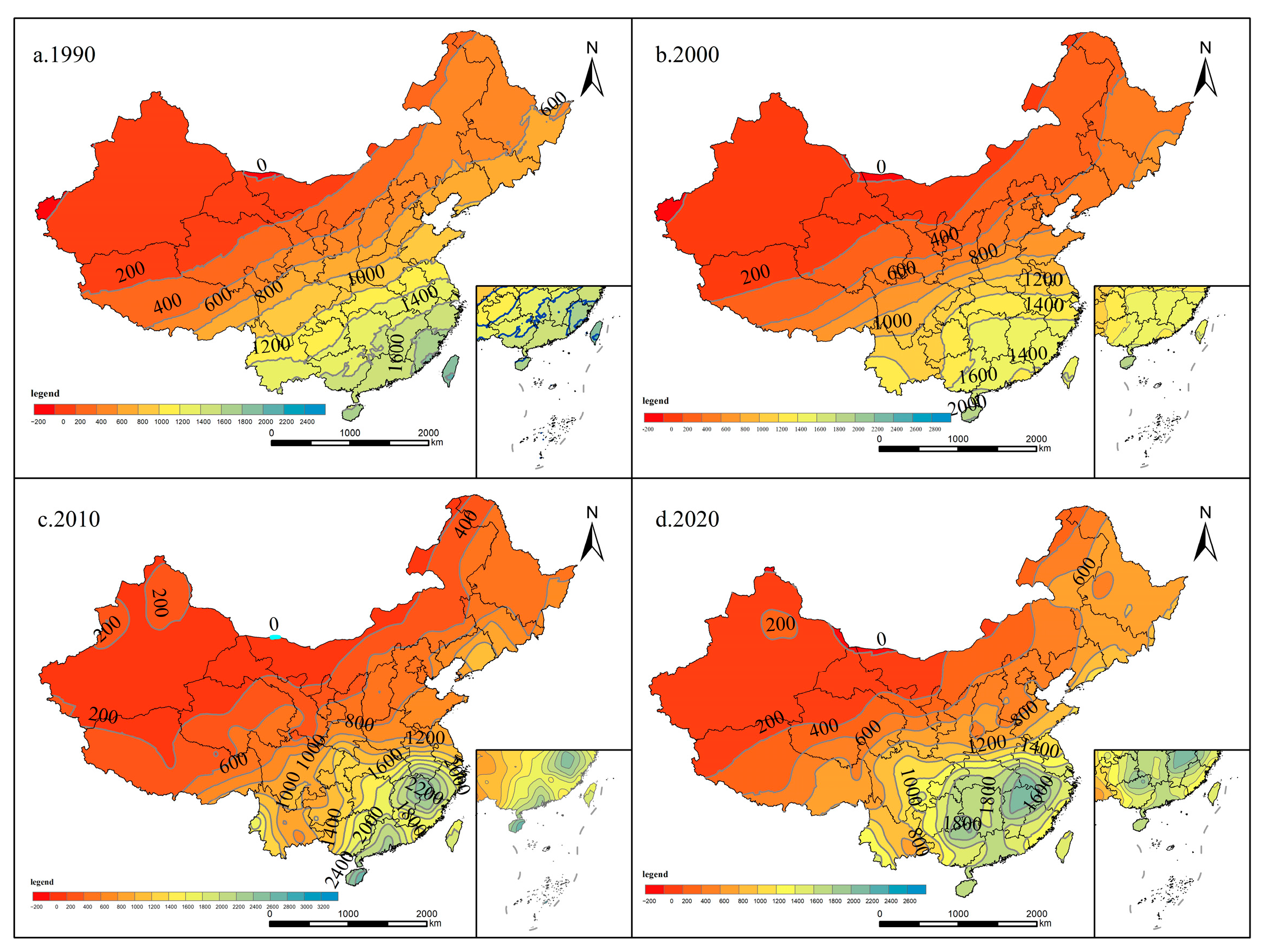
3.2. Distribution of Annual Total Isohyet

Based on the annual precipitation data from 1990, 2000, 2010, and 2020, the isopleth maps of annual precipitation are shown in Figure 3. As shown in Figure 3a, in 1990, the isohyets are generally distributed parallel, increasing from northwest to southeast. The 400 mm isohyet passes through the central part of Tibet, southern Qinghai, and the northern parts of Gansu, Ningxia, Shaanxi, Inner Mongolia, and Heilongjiang. The 800 mm isohyet passes through the southern parts of Tibet, Shaanxi and Liaoning, central Sichuan, and northern parts of Henan and Shandong. The 1600 mm isohyet is generally distributed along the provincial boundary of Fujian. The highest precipitation isohyet is approximately 2400 mm, located in the Hainan region.

As shown in Figure 3b, compared to 1990, in 2000, the 200 mm–1000 mm isohyets have shifted southward. The 200 mm isohyet has moved southward in the Inner Mongolia region, while the 400 mm isohyet passed through the southern parts of Gansu, Ningxia, Shaanxi, Shanxi, Beijing, Liaoning, Jilin, and Heilongjiang provinces. This line has shifted significantly southward in the central and eastern parts. The eastern part of the 800 mm isohyet has shifted southward to the southern tip of Shandong Province. The western segment of the 1200 mm isohyet has also shifted southward to the southern tip of Yunnan Province.

As shown in Figure 3c, compared to the previous two periods, the annual isohyets in 2010 are more complex, with an overall increasing trend from northwest to southeast. In the northwest, a 200 mm closed isohyet appears in the low-value area. The eastern section of the 400 mm isohyet has shifted slightly northward. The spacing between the 800 mm, 1000 mm, and 1200 mm isohyets has decreased and become more concentrated, particularly in Henan, Shaanxi, and Hubei provinces. Within the range of the 1000 mm to 1200 mm isohyets on the Yunnan-Guizhou Plateau, there are complex low-value enclosed areas of 600 mm and 800 mm isohyets, mainly concentrated in Yunnan Province. In the southeastern region, high precipitation areas are present in Guangxi, Guangdong, Jiangxi, southern Anhui, and Zhejiang provinces, with closed isohyetal areas above 2000 mm. Overall, the 400 mm and 800 mm isohyets have shown relatively smaller shifts, yet have a southward movement compared to 1990.

As shown in Figure 3d, compared with 1990, the overall isohyets in 2020 have shifted northward (details illustrated in Figure 4). The 200 mm isohyet is truncated in the middle section in northern Inner Mongolia. The 0–200 mm precipitation area is mainly concentrated in the northern parts of Tibet, Xinjiang, Qinghai, and Gansu, and western Inner Mongolia. The eastern section of the 400 mm isohyet has also shifted northward, passing through Ningxia, Shaanxi, Hebei, and the northern part of Heilongjiang. The 800 mm isohyet generally follows the same direction as the Yellow River, but its middle section aligns more closely with the latitude lines, with a small curvature. The density of the 800 mm–1400 mm isohyets has increased, concentrated between the Yellow River and the Yangtze River basins. A high-value area appears in the southern region. A closed 1800 mm isohyet area appears in the Yunnan-Guizhou Plateau. The border area between Jiangxi, Zhejiang, Anhui, and the southeastern part of Hubei is a closed 2000 mm isohyet area. In the southern coastal region, the 1400 mm isohyet is distributed along the eastern part of Guangdong, central Fujian, and the southern part of Zhejiang.

3.3. Distribution of Land Cover

Based on the land cover distribution data from 1990, 2000, 2010, and 2020, the summary table of land use types for each year (

Table 1. Summary of Land Use Type Area for Each Year unit: 10,000 km².

Year	Cropland	Forest	Shrub	Grassland	Water	Impervious	Wetland
1990	245.94	284.15	5.65	365.51	16.20	13.39	1.17
2000	243.70	288.12	4.39	357.57	16.91	18.98	0.36
2010	236.67	292.26	4.17	358.58	18.47	24.91	0.23
2020	236.05	294.07	3.46	352.41	18.71	31.38	0.24

) is created.

The area of cropland shows a decreasing trend. In 1990, the area of cropland was approximately 2.4594 million km², primarily distributed in the central and eastern plains, as well as the northeastern regions. By 2020, the area of cropland had decreased to 2.3605 million km², with a total reduction of about 98,900 km². Forests are mainly concentrated in the southern and northeastern parts of China, with a distribution range consistent with that of shrubs and showing an increasing trend in such areas. In 1990, the area of forests was approximately 2.8415 million km². By 2020, it had increased to about 2.9407 million km², representing a total increase of 99,200 km². The area of shrubs showed a decreasing trend, with a total reduction of approximately 21,900 km². The area of grassland and wetland presented a fluctuating decrease. To be precise, the grassland decreased by 131,000 km², while the wetland decreased by 9300 km². Both the area of water and the area of impervious surfaces showed an increasing trend, with the former up by 25,100 km², while the latter by 179,900 km².

3.4. Analysis of Driving Factors

3.4.1. Pearson Correlation Analysis

Meteorological factors have changed significantly over the past 30 years. Under the influence of temperature and precipitation, the distribution and pattern of land use have changed accordingly. This study has selected climate factors, such as the annual average temperature (TAVG/°C), annual precipitation (PRCP/mm), and sunshine hours (SUN/h), from 1990 to 2020 to further explore their influence on land use. The area of each land use type over the past 30 years is used as an indicator of land use evolution, and the correlation between meteorological factors and land use is analyzed.

The results of the Pearson correlation analysis are shown in

Table 2. Pearson Correlation Coefficients.

	PRCP(mm)	TAVG (°C)	SUN (h)	Cropland	Forest	Shrub	Grassland	Water	Impervious	Wetland
PRCP(mm)	1 (***)
TAVG(°C)	−0.35 (*)	1 (***)
SUN(h)	0.332	−0.283	1 (***)
Cropland	−0.209	0.549 (***)	0.068	1 (***)
Forest	0.305	−0.665 (***)	0.018	−0.955 (***)	1 (***)
Shrub	−0.441 (**)	0.787 (***)	−0.193	0.809 (***)	−0.904 (***)
Grassland	−0.423 (**)	0.87 (***)	−0.318	0.585 (***)	−0.742 (***)	0.916 (***)	1 (***)
Water	0.2	−0.64 (***)	0	−0.956 (***)	0.889 (***)	−0.823 (***)	−0.64 (***)	1 (***)
Impervious	0.397 (*)	−0.801 (***)	0.131	−0.881 (***)	0.939 (***)	−0.975 (***)	−0.879 (***)	0.902 (***)	1 (***)
Wetland	−0.118	0.483 (**)	0.051	0.86 (***)	−0.727 (***)	0.676 (***)	0.487 (**)	−0.949 (***)	−0.773 (***)	1 (***)

***, **, and * represent significance levels of 1%, 5% and 10%, respectively; PRCP stands for annual precipitation, TAVG stands for annual temperature, and SUN stands for sunshine hours.

. Precipitation shows significant correlation coefficients with three land use types: shrub (−0.441), grassland (−0.423), and impervious surfaces (0.397), with negative correlations for both shrubs and grassland. Temperature demonstrates strong correlations with grassland (0.87), impervious surfaces (−0.801), and shrubs (0.787), exhibiting a distinct negative correlation with impervious surfaces. Sunshine duration displays considerable correlation with shrubs, grassland, and impervious surfaces, in particular, showing a strong positive correlation with impervious surfaces.

The annual average temperature (TAVG/°C) shows a stronger correlation with land use types compared to precipitation (PRCP/mm) and sunshine hours (h), especially with grassland, impervious surfaces, and shrubs, where the correlation coefficients are all above 0.75, indicating a significant correlation. Since the value of the Pearson correlation coefficient can be affected by the sample size, smaller sample sizes can lead to larger fluctuations in the correlation coefficient. To further explore the degree of correlation between meteorological factors and land use types, it is necessary to apply other methods and models for deeper exploration and verification. Therefore, this study uses grey relational analysis and the VAR model to further assess the extent and contribution of meteorological factors on land use.

3.4.2. Grey Correlation Analysis

According to the correlation degree ranking table of precipitation, temperature, sunshine hours, and land use types (

Table 3. Correlation Degree between Precipitation, Temperature, Sunshine Hours, and Land Use Types.

	PRCP		TAVG		SUN
Evaluation Item	Correlation Degree	Ranking	Correlation Degree	Ranking	Correlation Degree	Ranking
Forest	0.896	1	0.905	3	0.912	1
Water	0.889	2	0.848	5	0.892	4
Grassland	0.882	3	0.932	2	0.905	2
Cropland	0.877	4	0.933	1	0.895	3
Shrub	0.797	5	0.889	4	0.802	5
Impervious	0.742	6	0.659	7	0.681	6
Wetland	0.707	7	0.706	6	0.641	7

), the land use types ranked by their correlation with precipitation in a descending order are as follows: forests, water, grassland, cropland, shrubs, impervious surfaces, and wetland. The correlation degree between forests and precipitation is the highest, with a value of 0.896, while it is the lowest between wetland and precipitation, with a value of 0.707. The land use types ranked by their correlation with the annual average temperature in a descending order are as follows: cropland, grassland, forests, shrubs, water, wetland, and impervious surfaces. The correlation degree between cropland and the annual average temperature is the highest, with a value of 0.933, while the lowest value of 0.659 is found between impervious surfaces and the annual average temperature.

The land use types ranked by their correlation with sunshine hours are as follows: forests, grassland, cropland, water, shrubs, impervious surfaces, and wetland. The correlation degree between forest and sunshine hours is the highest, with a value of 0.912, while the lowest value of 0.641 happens between wetland and sunshine hours.

3.4.3. Impulse Response Analysis Based on the VAR Model

The results of the grey relational analysis show that the top four land use types with the highest correlation degrees to meteorological factors discussed herein are forests, grassland, cropland, and water. Sequentially, one indicator from the land use types of cropland, forest, grassland, and water will be selected. Then, VAR models will be established for each of these indicators in relation to these meteorological factors.

(1)

Lag Order Analysis

VAR models established for cropland, forests, grassland, and water with meteorological factors will be referred to as VAR01, VAR02, VAR03, and VAR04, respectively. First, the lag order for the models needs to be determined. The test values are shown in

Table 4. Lag Order Analysis of Different Land Types and Annual Mean Temperature, Precipitation, and Sunshine Hours.

Class of Land	Order Number	AIC	BIC	FPE	HQIC
Cropland	0	50.416	50.615	7.86 × 1021	50.459
	1	47.081	48.076 *	2.9 × 1020	47.297
	2	46.878	48.669	2.89 × 1020	47.267
	3	45.918 *	48.504	2.02 × 1020 *	46.479 *
Forest	0	49.786	49.985	4.19 × 1021	49.829
	1	46.686	47.681 *	1.96 × 1020	46.902
	2	46.287	48.078	1.6 × 1020	46.676
	3	45.146 *	47.733	9.32 × 1019 *	45.707 *
Grassland	0	49.148	49.347	2.21 × 1021	49.192
	1	47.076	48.070	2.89 × 1020	47.291
	2	46.097 *	47.888 *	1.33 × 1020 *	46.486 *
	3	46.604	49.190	4.01 × 1020	47.165

* stands for the order of the resolution, AIC stands for Akaike information criterion, BIC stands for Bayesian information criterion, FPE stands for final prediction error, and HQIC stands for Hannan-Quinn Information Criterion. In Vector Autoregression (VAR) models, they are employed to determine the lag order. Under different information criteria, the lag order corresponding to the minimum value is selected as the lag order of the model.

. The lag order of the model is determined by the lag number corresponding to the minimum value of the test statistics. Under different criteria, the lag order with the smallest value is taken as the final criterion. Since the VAR04 model failed the stationary test, it would be inapplicable to determine the lag order for this model. Therefore, VAR04 is considered not to be reasonable. As a result, lag order analysis is only conducted for the VAR01, VAR02, and VAR03 models, with lag orders of 1, 1, and 2, respectively.

(2)

VAR Model Parameter Estimation

After determining the lag order, parameter estimation is performed for the established VAR models. The results are shown in

Table 5. Parameter Estimation of VAR01 Model.

Indicators	Cropland	TAVG (°C)	PRCP (mm)	SUN (h)
Constant	115,791,048.891	−5.242	1277.066	−308.888
	(0.994)	(−0.909)	(1.829)	(−0.079)
L1 Cropland	0.972 **	0.000	0.000	0.000
	(19.446)	(1.837)	(0.298)	(1.122)
L1 TAVG (°C)	−3,462,212.556	0.617 **	−40.557 *	−175.015
	(−1.040)	(3.746)	(−2.033)	(−1.560)
L1 PRCP (mm)	20,631.250	−0.003	−0.290	0.166
	(0.545)	(−1.368)	(−1.277)	(0.130)
L1 SUN (h)	−3621.175	0.000	−0.043	−0.149
	(−0.491)	(0.508)	(−0.984)	(−0.602)

* means p < 0.05, ** means p < 0.01, the t value is in parentheses, PRCP means precipitation, TAVG means average annual temperature.

,

Table 6. Parameter Estimation of VAR02 Model.

Indicators	Forest	TAVG (°C)	PRCP (mm)	SUN (h)
Constant	−135,566,461.890	34.812 *	514.636	12,026.825
	(−0.546)	(2.458)	(0.292)	(1.189)
L1 Forest	1.029 **	−0.000 *	0.000	−0.000
	(15.542)	(−2.204)	(0.546)	(−0.848)
L1 TAVG (°C)	2,601,863.612	0.535 **	−29.518	−174.012
	(0.850)	(3.062)	(−1.358)	(−1.395)
L1 PRCP (mm)	5892.773	−0.002	−0.309	0.208
	(0.185)	(−1.259)	(−1.364)	(0.160)
L1 SUN (h)	1252.559	0.000	−0.033	−0.126
	(0.204)	(0.473)	(−0.748)	(−0.504)

* means p < 0.05, ** means p < 0.01, the t value is in parentheses, PRCP means precipitation, TAVG means average annual temperature.

and

Table 7. Parameter Estimation of VAR03 Model.

Indicators	Grassland	TAVG (°C)	PRCP (mm)	SUN (h)
Constant	1,147,261,817	−4.613	4693.669	−20,655.047
	(1.891)	(−0.143)	(1.671)	(−1.051)
L2 Grassland	−0.698 **	−0.000	−0.000	0.000 *
	(−2.912)	(−1.369)	(−0.323)	(2.313)
L2 TAVG (°C)	13,144,985.009 *	0.315	−46.521	−620.418 **
	(2.207)	(0.998)	(−1.687)	(−3.216)
L2 PRCP (mm)	−131,017.355 **	−0.002	0.042	1.116
	(−3.371)	(−0.791)	(0.235)	(0.886)
L2 SUN (h)	5074.483	0.000	0.018	−0.142
	(0.739)	(0.880)	(0.562)	(−0.640)

* means p < 0.05, ** means p < 0.01, the t value is in parentheses, PRCP means precipitation, TAVG means average annual temperature.

.

(3)

Model Stationary Test

The model stationary test is based on whether the reciprocals of the roots of the AR characteristic polynomial lie within the unit circle. If all the roots lie within the unit circle, the model is considered stationary, indicating that it satisfies the conditions for stability. If any root falls outside the unit circle, the model may not possess long-term stability. From the test results (Figure 5), it can be seen that both the VAR01 and VAR02 models have passed the AR root test. However, the characteristic root of the VAR03 model lies outside the unit circle, suggesting that this model may not possess long-term stability and thus is considered meaningless. Therefore, impulse response and variance decomposition analyses are only conducted for the VAR01 and VAR02 models.

From the impulse response results (Figure 6), it can be observed that, apart from the self-response values, changes in annual average temperature, precipitation, and sunshine hours have either positive or negative effects on cropland and forests. This indicates that the three meteorological factors have varying degrees of influence on the evolution of cropland and forests. For the changes in cropland, the response value to the annual average temperature is relatively high and negative, gradually converging as the number of lags increases. Precipitation shows a slight positive response, while sunshine hours exhibit a slight negative response. For the changes in forests, the response value to the annual average temperature is relatively high and positive, tending to stabilize as the number of lags increases. Unlike cropland, during the changes in forests, precipitation shows a slight negative response, while sunshine hours exhibit a slight positive response.

The impulse response results for both land types indicate that, compared to other meteorological factors, the annual average temperature has a more significant impact on the changes in both cropland and forests. Furthermore, the two land types exhibit opposing trends: changes in annual average temperature have a negative driving effect on cropland but a positive driving effect on forests. To explore the contribution of meteorological factors to the changes in cropland and forests, variance decomposition is further employed to conduct the contribution analysis.

From the variance decomposition results in Figure 7a,b, it can be seen that, apart from their own contributions, the annual average temperature (TAVG/°C) contributes the most to the changes in both cropland and forests. For cropland, the contribution of annual average temperature gradually stabilizes after the 8th period, exceeding 8%, while precipitation and sunshine hours contribute only 1.0% and 1.6%, respectively, which is much smaller. For forests, the contributions of the three meteorological factors are relatively low. To be precise, the contribution of the annual average temperature stabilizes after the 7th period, exceeding 3.0%. Whereas, the contributions of precipitation and sunshine hours remain below 0.3% throughout the 10 periods, making them negligible.

In summary, the annual average temperature remains the greatest contributor to the changes in both cropland and forests among all meteorological factors. It can be further observed that it has a stronger driving effect on the evolution of cropland.

4. Discussion

The mean temperature in China has exhibited a consistent upward trend over the past few decades. Between 1980 and 2020, there was a recorded increase of 0.319 °C [4], with an average warming rate of approximately 0.28 °C per decade [2,38]. This investigation demonstrates fluctuations and overall escalation in the average annual temperature over the last 30 years. Specifically, the area with temperatures above 20 °C has expanded in the southern region, accompanied by a northward shift of the 10 °C and 15 °C isotherms (see Figure 2). Several studies have highlighted a rise in precipitation across China, particularly in the southeast and the Yangtze River Basin, with an average annual growth rate of about 0.049 mm [3,4,39]. The findings of this study confirm the observed increase in precipitation throughout China, resulting in a general northward shift of the isohyet (refer to Figure 4), albeit with regional disparities. Notably, the southeastern area has experienced a pronounced northward shift and an expansion of the 1600 mm isohyet, while the northwest region has shown comparatively minor changes. The spatial distribution differences between isotherms and isohyets may be related to factors such as economic development and geographic location. In the southeastern region, proximity to the ocean enhances maritime influence, while monsoon circulation transports abundant moisture, leading to significantly increased precipitation. Conversely, areas farther inland experience diminished oceanic effects. Additionally, topography plays a critical role: the southeastern region’s hilly and flat terrain facilitates upward moisture movement and precipitation, whereas northwestern mountain ranges block moisture transport. Furthermore, the southeast’s developed economy and higher population density intensify urban heat island effects compared to the northwest, which also contributes to local variations in temperature and precipitation patterns [40].

Variations in temperature and precipitation impact vegetation growth and soil moisture by altering hydrothermal conditions and the spatial distribution and availability of water resources, thereby influencing land use dynamics [41,42]. Our research reveals a significant negative correlation between temperature changes and cropland transformation, with temperature accounting for up to 8% of the variance. Rising temperatures enhance soil evaporation, cropland transpiration, and alter vegetation patterns, leading to the deterioration of cropland and grassland in arid and semi-arid regions [43]. Specifically, the cropland decreased by approximately 100,000 km², and the grassland area diminished by approximately 130,000 km² in our analysis. In regions without irrigation, extreme heat can diminish cropland productivity, resulting in reduced cropland extent [44,45]. Concurrently, temperature elevation fosters forest expansion, as forest growth is contingent upon accumulated temperatures, promoting forest migration to higher latitudes and elevations [46,47].

The impact of precipitation variability on land use is multifaceted and varies across regions, primarily altering the availability of water resources, soil moisture levels, and vegetation growth conditions [48,49,50]. Land use changes are influenced by a variety of factors, and in the context of climate change, the area of cropland has decreased, and the area of forested land has increased due to the effects of temperature and precipitation. Elevated precipitation levels have the potential to induce flooding, exacerbate soil erosion, and result in the degradation of cultivated areas, ultimately diminishing soil fertility [51,52]. Simultaneously, it can enhance forest growth by ameliorating water conditions [53]. Variations in precipitation can also impact cropland through alterations in land use categories. In the Yellow River Basin, heightened precipitation results in wetland expansion and cropland reduction [54]. In arid and semiarid areas, increased precipitation fosters greater forest coverage [3]. Climate change has induced modifications in climatic zones and eco-geographical regions in China to a certain extent [5]. The impact of climate change on land use alteration varies across regions, necessitating region-specific measures to address climate change, optimize land utilization, and safeguard the ecological environment.

This study focused on meteorological factors, specifically temperature and precipitation, while the distinct impacts of economic and policy factors were not quantified. Future research could develop a comprehensive model by integrating data from various sources. We did not include land conversion in our model for analyzing changes in land area. This may have led to a similar decrease in grassland and shrub, which should have replaced degraded cropland. This phenomenon may also be related to uncertainty in land classification.

5. Conclusions

(1)

From 1990 to 2020, annual mean isotherms and isohyets shifted northward, with notable migration of the 10 °C and 15 °C isotherms. The 1600 mm isohyet experienced the most pronounced northward expansion, while the 800–1200 mm isohyets migrated northwestward with contracted intervals.

(2)

The overall trend shows a decrease in the areas of cropland, shrubs, grassland, and wetland, with a cropland decrease of about 100,000 km². In contrast, the areas of forests, water, and impervious surfaces have increased year by year. Forests expanded by approximately 100,000 km², while impervious surfaces experienced the largest increase, reaching approximately 180,000 km².

(3)

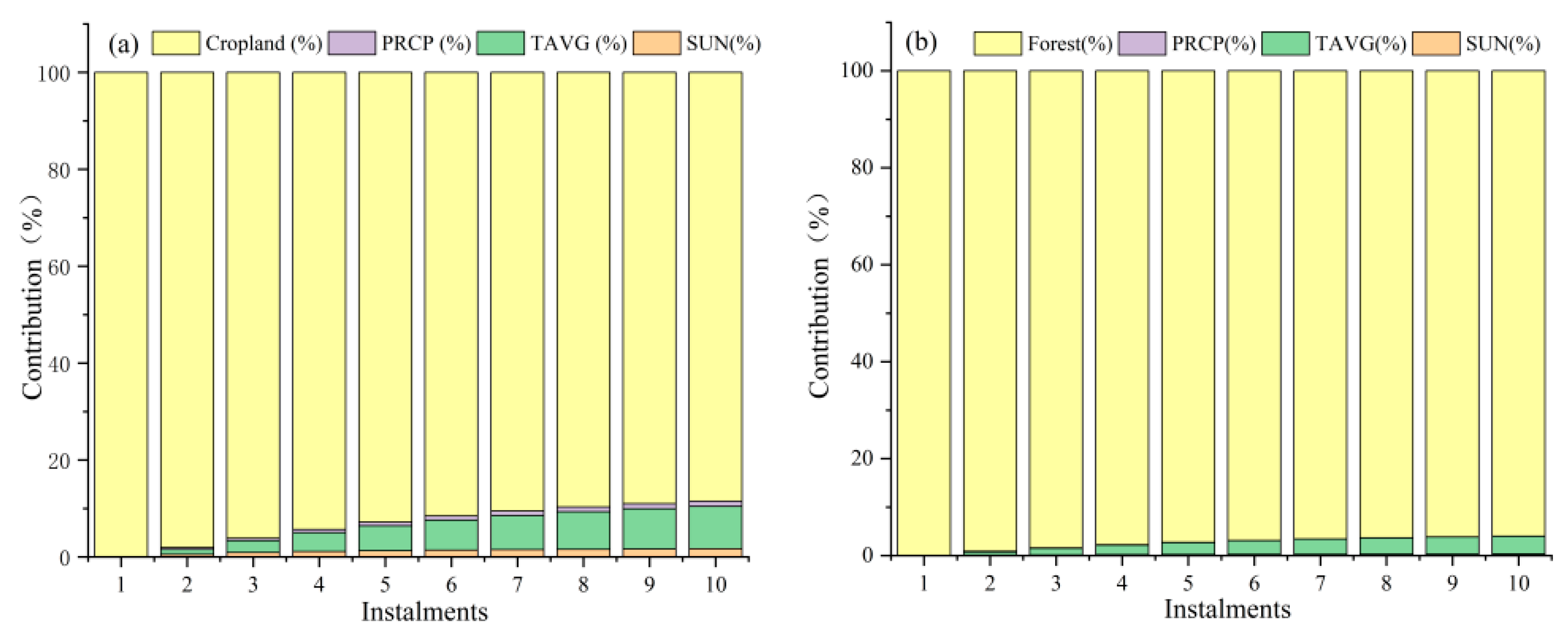
Among the meteorological factors, the annual average temperature shows a strong correlation with land use changes. Changes in annual average temperatures have a negative driving effect on cropland, but a positive driving effect on forests. Specifically, for cropland, the contribution of annual average temperature exceeded 8% after the 8th period.

References

1. Gao, Q.; Qin, Y.; Liang, M.; Gao, X. Interpretation of the main conclusions and suggestions of IPCC AR6 synthesis report. Environ. Prot. 2023, 51, 82–84. [Google Scholar] [CrossRef]
2. Jiang, P.; Pan, X.M.; Zeng, X.Y. Temporal and Spatial Variation of Temperature and Precipitation in Each Agricultural Sub-region of China. Res. Soil Water Conserv. 2020, 27, 270–278. [Google Scholar] [CrossRef]
3. Chen, S.; Zhao, W.; Han, Y. Spatio-temporal variation of vegetation precipitation use efficiency and influencing factors in arid and semi-arid areas of China. Acta Ecol. Sin. 2023, 43, 10295–10307. [Google Scholar] [CrossRef]
4. Xu, M. Climate Change in China: An Analysis of Temperature and Precipitation Variations Across 2367 Meteorological Stations (1981–2020). Highlights Sci. Eng. Technol. 2024, 88, 430–438. [Google Scholar] [CrossRef]
5. Wang, F.; Li, B.; Tian, S.; Zheng, D.; Ge, Q. Updated scheme for eco-geographical regionalization in China. Acta Geogr. Sin. 2024, 79, 3–16. [Google Scholar]
6. Tran, T.-N.-D.; Tapas, M.R.; Do, S.K.; Etheridge, R.; Lakshmi, V. Investigating the impacts of climate change on hydroclimatic extremes in the Tar-Pamlico River basin, North Carolina. J. Environ. Manag. 2024, 363, 121375. [Google Scholar] [CrossRef]
7. Tran, T.N.; Lakshmi, V. Enhancing human resilience against climate change: Assessment of hydroclimatic extremes and sea level rise impacts on the Eastern Shore of Virginia, United States. Sci. Total Environ. 2024, 947, 174289. [Google Scholar] [CrossRef]
8. Franzke, C.L.E.; Lee, J.-Y.; O’Kane, T.; Merryfield, W.; Zhang, X. Extreme Weather and Climate Events: Dynamics, Predictability and Ensemble Simulations. Asia-Pac. J. Atmos. Sci. 2023, 59, 1–2. [Google Scholar] [CrossRef]
9. Rafiei-Sardooi, E.; Azareh, A.; Shooshtari, S.J.; Parteli, E.J.R. Long-term assessment of land-use and climate change on water scarcity in an arid basin in Iran. Ecol. Model. 2022, 467, 109934. [Google Scholar] [CrossRef]
10. Chegnizadeh, A.; Rabieifar, H.; Ebrahimi, H.; Nayeri, M.Z. Evaluating The hydrological response due to the changes in climate and land use on streamflow in the Karkheh basin, Iran. J. Water Clim. Change 2022, 13, 4054–4068. [Google Scholar] [CrossRef]
11. Huang, J.; Deng, X.; Qi, Y.; Wang, P.; Jian, Y. Impact of Climate Change and Human Activities on the Changes in Net Primary Ecosystem Productivity in Henan Province. Environ. Sci. 2025, 1–20. [Google Scholar] [CrossRef]
12. Cui, N.; Yin, Q. Impacts of Climate Change on Grain Production in Northeast China and Countermeasures. J. Catastrophology 2022, 37, 52–57. [Google Scholar]
13. Zhao, H.; Cui, Y.; Li, M.; Kang, X.; Li, W.; Han, Y.; Yang, J.; Wang, Y. Impacts of climate change and human activities on net primary productivity of vegetation in Ningxia, Northwest China. Chin. J. Appl. Ecol. 2025, 1–16. [Google Scholar] [CrossRef]
14. Zewdu, D.; Krishnan, C.M.; Raj, P.P.N.; Makadi, Y.C.; Barati, M.K.; Arlikatti, S. Interactions of land use, land cover, and climate change: A case study of Raichur District, Karnataka, India. Environ. Chall. 2025, 19, 101166. [Google Scholar] [CrossRef]
15. Kennedy, J.; Hurtt, G.C.; Liang, X.-Z.; Chini, L.; Ma, L. Changing cropland in changing climates: Quantifying two decades of global cropland changes. Environ. Res. Lett. 2023, 18, 064010. [Google Scholar] [CrossRef]
16. Ding, X.; Ye, C. Eco-environmental effects of ‘production-cology-living’ land use transformation and the analysis of terrain gradient in poyang lake city cluster. Res. Soil Water Conserv. 2024, 31, 315–326. [Google Scholar] [CrossRef]
17. Zhao, Y.; Cao, H.; Yang, J.; Jiang, Y.; Zhang, R. Land use pattern and multifunctional spatiotemporal evolution in the northwest plateau of sichuan based on “production-living-ecosystem” space. Sci. Technol. Manag. Land Resour. 2022, 39, 1–14. [Google Scholar]
18. Lou, J.; Dang, X.; Meng, Z.; Zhang, H.; Song, H. Land use change and driving force analysis of the ten tributaries basin in the yellow river basin from 1986 to 2020. J. Soil Water Conserv. 2024, 38, 319–327+336. [Google Scholar] [CrossRef]
19. Liao, W.; Liu, X.; Xu, X.; Chen, G.; Liang, X.; Zhang, H.; Li, X. Projections of land use changes under the plant functional type classification in different SSP-RCP scenarios in China. Sci. Bull. 2020, 65, 1935–1947. [Google Scholar] [CrossRef]
20. Kirti, C.; Dhrubajyoti, S.; Jatan, D. Assessment of the land use/land cover and climate change impact on the hydrological regime of the Kulsi River catchment, Northeast India. Sustain. Water Resour. Manag. 2024, 10, 60. [Google Scholar]
21. Quan, L.a.; Jin, S.; Chen, J.; Li, T. Evolution and Driving Forces of Ecological Service Value in Anhui Based on Landsat Land Use and Land Cover Change. Remote Sens. 2024, 16, 269. [Google Scholar] [CrossRef]
22. Ning, J.; Liu, J.Y.; Kuang, W.H.; Xu, X.L.; Zhang, S.W.; Yan, C.Z.; Li, R.D.; Wu, S.X.; Hu, Y.F.; Du, G.M.; et al. Spatiotemporal patterns and characteristics of land-use change in China during 2010–2015. J. Geogr. Sci. 2018, 28, 547–562. [Google Scholar] [CrossRef]
23. Perring, M.P.; Pieter, D.F.; Lander, B.; Maes, S.L.; Leen, D.; Haben, B.; Carón, M.M.; Kris, V. Global environmental change effects on ecosystems: The importance of land-use legacies. Glob. Change Biol. 2016, 22, 1361–1371. [Google Scholar] [CrossRef] [PubMed]
24. Liao, M.; Fang, X.; Jiang, X.; Zhu, Q.; Jin, J.; Ren, L.; Yan, Y. Spatiotemporal characteristics of land use/cover changes in the Yellow River Basin over the past 40 years. J. Soil Water Conserv. 2024, 38, 165–177+189. [Google Scholar] [CrossRef]
25. Huang, Y.; Li, X.; Yu, Q.; Huang, H. An analysis of land use change and driving forces in the Yellow River Basin from 1995 to 2018. J. Northwest For. Univ. 2022, 37, 113–121. [Google Scholar]
26. Gao, X.; Cheng, W.; Wang, N.; Liu, Q.; Ma, T.; Chen, Y.; Zhou, C. Spatio-temporal distribution and transformationof cropland in geomorphologic regions of China during 1990–2015. J. Geogr. Sci. 2019, 29, 180–196. [Google Scholar] [CrossRef]
27. Zhang, X.; Ceng, Y.; Gao, Z.; Li, Y.; Sun, G.; Liu, W. Response of eco-environmental quality to climate change and land use in Loess Plateau from 2000 to 2020. Bull. Soil Water Conserv. 2023, 43, 234–244. [Google Scholar] [CrossRef]
28. Yang, J.; Huang, X. The 30m annual land cover dataset and its dynamics in China from 1990 to 2019. Earth Syst. Sci. Data 2021, 13, 3907–3925. [Google Scholar] [CrossRef]
29. Samyuktha, N.; Rao, P.J.; Ramu, N. Correlation analysis of land surface temperature on landsat-8 data of Visakhapatnam Urban Area, Andhra Pradesh, India. Earth Sci. Inform. 2022, 15, 1963–1975. [Google Scholar]
30. Wu, Q.; Tan, J.; Guo, F.; Li, H.; Chen, S. Multi-scale relationship between land surface temperature and landscape pattern based on wavelet coherence: The case of metropolitan Beijing, China. Remote Sens. 2019, 11, 3021. [Google Scholar] [CrossRef]
31. Chen, X.; Jiang, H.; Cheng, H.; Zheng, H. Application of Correlation Analysis Based on Principal Components in the Study of Global Temperature Changes. Iran. J. Energy Environ. 2023, 14, 336–345. [Google Scholar] [CrossRef]
32. Zhao, Y.; Zhang, Y.; Yang, Y.; Li, F.; Dai, R.; Li, J.; Wang, M.; Li, Z. The Impact of Land Use Structure Change on Utilization Performance in Henan Province, China. Int. J. Environ. Res. Public Health 2023, 20, 4251. [Google Scholar] [CrossRef] [PubMed]
33. Bai, J.; Zhou, Z.; Zou, Y.; Bakhtiyor, P.; Siddique, K.H.M. Watershed drought and ecosystem services: Spatiotemporal characteristics and gray relational analysis. ISPRS Int. J. Geo-Inf. 2021, 10, 43. [Google Scholar] [CrossRef]
34. Li, X.; Xu, X.; Wang, X.; Xu, S.; Tian, W.; Tian, J.; He, C. Assessing the effects of spatial scales on regional evapotranspiration estimation by the SEBAL Model and multiple satellite datasets: A case study in the agro-pastoral ecotone, Northwestern China. Remote Sens. 2021, 13, 1524. [Google Scholar] [CrossRef]
35. Fayyaz, S.; Moeinaddini, M.; Pourebrahim, S.; Khoshnevisan, B.; Kazemi, A.; Toufighi, S.P.; Schjønberg, M.S.; Birkved, M. Assessing environmental enhancement scenarios in a petrochemical port: A comprehensive comparison using a hybrid LCA-GRM model. J. Clean. Prod. 2024, 445, 141079. [Google Scholar] [CrossRef]
36. Babalos, V.; Stavroyiannis, S. Pension funds and stock market development in OECD countries: Novel evidence from a panel VAR. Financ. Res. Lett. 2020, 34, 101247. [Google Scholar] [CrossRef]
37. Cornell, C.; Mitchell, L.; Roughan, M. Rank is all you need: Development and analysis of robust causal networks. Appl. Netw. Sci. 2024, 9, 39. [Google Scholar] [CrossRef]
38. Fan, Z.; Yue, T.; Chen, C.; Sun, X. Spatial Change Trends of Temperature and Precipitation in China. J. Geo-Inf. Sci. 2011, 13, 526–533. [Google Scholar] [CrossRef]
39. Zhang, Y.; Zang, S.; Shen, X.; Fan, G. Observed Changes of Rain-Season Precipitation in China from 1960 to 2018. Int. J. Environ. Res. Public Health 2021, 18, 10031. [Google Scholar] [CrossRef]
40. Patil, R.; Surawar, M. Impact of Urban Heat Island on Formation of Precipitation in Indian Western Coastal Cities. J. Contemp. Urban Aff. 2023, 7, 38–55. [Google Scholar] [CrossRef]
41. Zhu, K.; Cheng, Y.; Zhou, Q.; Kápolnai, Z.; Dávid, L.D. The contributions of climate and land use/cover changes to water yield services considering geographic scale. Heliyon 2023, 9, e20115. [Google Scholar] [CrossRef] [PubMed]
42. Hu, X.; Yi, Y.; Kang, H.; Wang, B.; Shi, M.; Liu, C. Temporal and spatial variations of land use and the driving factors in the middle reaches of the Yangtze River in the past 25 years. Acta Ecol. Sin. 2019, 39, 1877–1886. [Google Scholar]
43. Huang, Y.; Li, G.; Zhao, Y.; Yang, J.; Li, Y. Analysis of the Characteristics and Causes of Land Degradation and Development in Coastal China (1982–2015). Remote Sens. 2023, 15, 2249. [Google Scholar] [CrossRef]
44. Gao, P.; Gao, Y.; Ou, Y.; McJeon, H.; Iyer, G.; Ye, S.; Yang, X.; Song, C. Heterogeneous pressure on croplands from land-based strategies to meet the 1.5 °C target. Nat. Clim. Change 2025, 15, 420–427. [Google Scholar] [CrossRef]
45. Wang, J.; Zhang, J.; Zhang, P. Rising temperature threatens China’s cropland. Environ. Res. Lett. 2022, 17, 084042. [Google Scholar] [CrossRef]
46. Wang, Y.; Zhang, J.; Liu, J.; Wang, L.; Li, Y. Research progress on cambium activity and radial growth dynamics monitoring of coniferous species. Chin. J. Appl. Ecol. 2024, 35, 1223–1232. [Google Scholar] [CrossRef]
47. Li, T.; Luo, P.; Xiong, Q.; Yang, H.; Gu, X.; Qiu, Y.; Lin, B.; Liu, Y.; Lai, C. Spatial heterogeneity of tree diversity response to climate warming in montane forests. Ecol. Evol. 2021, 11, 931–941. [Google Scholar] [CrossRef]
48. Baker, J.C.A.; Castilho de Souza, D.; Kubota, P.Y.; Buermann, W.; Coelho, C.A.S.; Andrews, M.B.; Gloor, M.; Garcia-Carreras, L.; Figueroa, S.N.; Spracklen, D.V. An Assessment of Land–Atmosphere Interactions over South America Using Satellites, Reanalysis, and Two Global Climate Models. J. Hydrometeorol. 2021, 22, 905–922. [Google Scholar] [CrossRef]
49. Wang, J.; Zhang, Q.; Peng, H.; Lyu, X. Impact of Individual Rainfall on the Changes of Soil Water Content in Deep Layer of Different Land Uses. Res. Soil Water Conserv. 2023, 30, 69–75. [Google Scholar] [CrossRef]
50. Luo, Y.; Liang, W.; Yan, J.; Zhang, W.; Gou, F.; Wang, C.; Liang, X. Vegetation Growth Response and Trends after Water Deficit Exposure in the Loess Plateau, China. Remote Sens. 2023, 15, 2593. [Google Scholar] [CrossRef]
51. Li, T.; Ma, F.; Wang, J.; Qiu, P.; Zhang, N.; Guo, W.; Xu, J.; Dai, T. Study on the Mechanism of Rainfall-Runoff Induced Nitrogen and Phosphorus Loss in Hilly Slopes of Black Soil Area, China. Water 2023, 15, 3148. [Google Scholar] [CrossRef]
52. Rupngam, T.; Messiga, A.J. Unraveling the Interactions between Flooding Dynamics and Agricultural Productivity in a Changing Climate. Sustainability 2024, 16, 6141. [Google Scholar] [CrossRef]
53. Xia, Z.; Xie, Y.; Wang, T. Land Use and Spatial and Temporal Change of Normalized Difference Vegetation Index(NDVI) in Shenfu Mining Area and Their Driving Factors Analysis. Chin. Agric. Sci. Bull. 2021, 37, 97–105. [Google Scholar]
54. Zhang, R.; Yan, F.; Xiao, S.; He, R. Precipitation Effects of Land Use Change in the Upper and Middle Reaches of the Yellow River Basin. J. Shanxi Agric. Sci. 2023, 51, 1078–1087. [Google Scholar]
Figure 1. Contour distribution of annual average temperatures in different years.
Land 14 01417 g001
Figure 2. Annual mean Isotherm variation.
Land 14 01417 g002
Figure 3. Contour distribution of annual precipitations in different years.
Land 14 01417 g003
Figure 4. Annual isohyet variation.
Land 14 01417 g004
Figure 5. AR root test results.
Land 14 01417 g005
Figure 6. Impulse response results.
Land 14 01417 g006
Figure 7. Variance decomposition results ((a) for cropland, (b) for forest).
Land 14 01417 g007