Figure 1.
Aggregated 6 × 6 land-use transition matrix based on IPCC land-use categories. The LUC matrix categorizes the area (ha) of land within each combination of land-use classes over the two years selected for the inventory period. Dark blue cells indicate land area that has not changed, while light blue cells indicate areas converted from one land use to another.
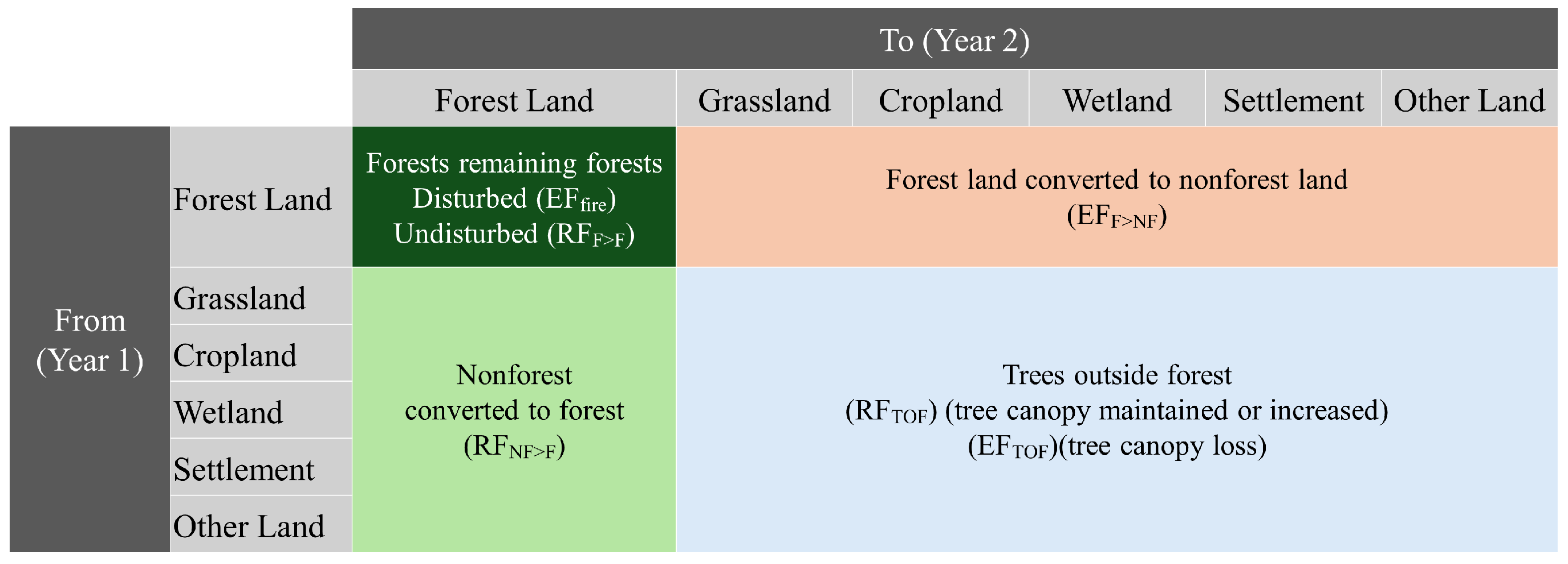
Figure 2.
Activity data categories from the IPCC land-use transition matrix recategorized into GHG reporting categories. EF = emission factor; RF = removal factor; F = forest; NF = nonforest; TOF = trees outside forest; F > F = forest remaining forest; F > NF = forest to nonforest; NF > F = nonforest to forest. “RF” corresponds to activity data that are paired with a removal factor, and “EF” corresponds to activity data that are paired with an emission factor.
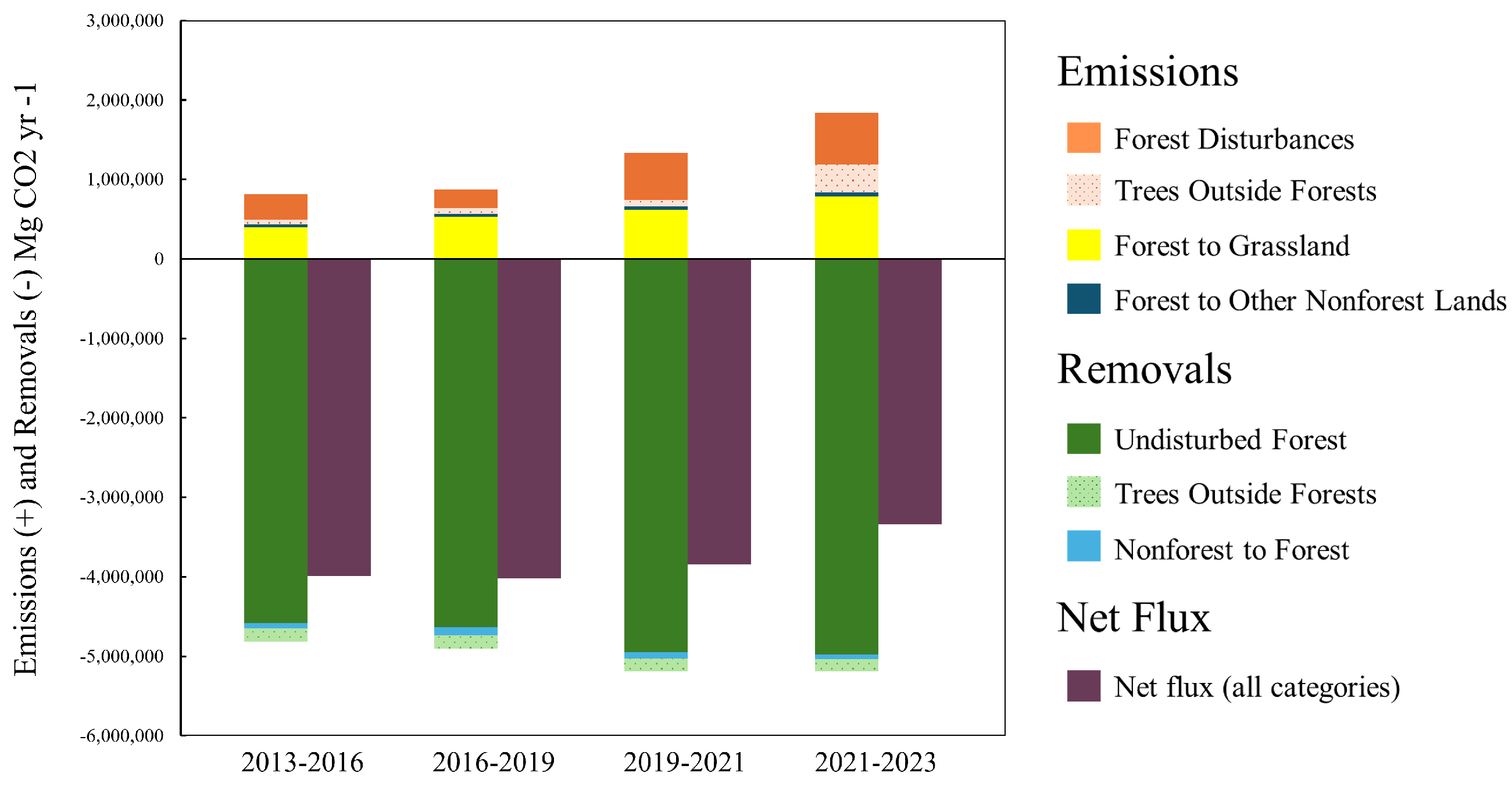
Figure 3.
Summary of emissions and removals for four successive time periods in Jefferson County, Washington. Stacked columns show gross emissions (positive values) and gross removals (negative values) by inventory period. Emissions result from forest disturbances, trees outside forests, and land-use transitions from forest to grassland and other nonforest land uses. Removals result from undisturbed forests, trees outside forests, and transitions from nonforest land uses to forest. Purple columns represent the overall net flux for the inventory period. All values are annual averages across the inventory period. All units in Mg CO2/year.
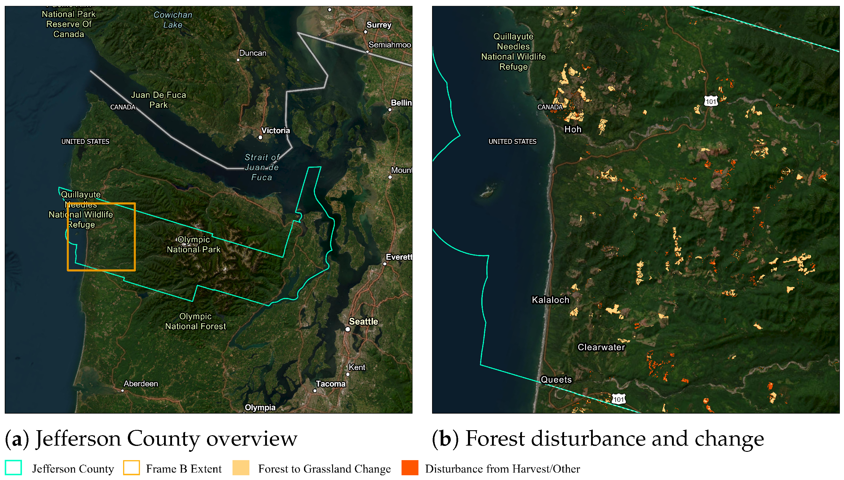
Figure 4.
Forest-to-grassland change and harvest disturbance (2019–2021) in Jefferson County. (a) County outline (cyan) with the zoom frame for panel (b) in orange. (b) Detail showing forest-to-grassland conversion (light orange) and harvest/other disturbance (dark orange). The legend applies to both panels. Service Layer Credits: Earthstar Geographics, WA State Parks GIS, Esri, TomTom, Garmin, SafeGraph, METI/NASA, USS, BLM, EPA, USDA, USFWS.
Figure 5.
Summary of emissions and removals for four successive time periods in Montgomery County, Maryland. Stacked columns show gross emissions (positive values) and gross removals (negative values) by inventory period. Emissions result from forest disturbances, trees outside forests, and land use transitions from forest to grassland and other nonforest land uses. Removals result from undisturbed forests, trees outside forests, and transitions from nonforest land uses to forest. Purple columns represent the overall net flux for the inventory period. All values are annual averages across the inventory period. All units in Mg CO2/year.
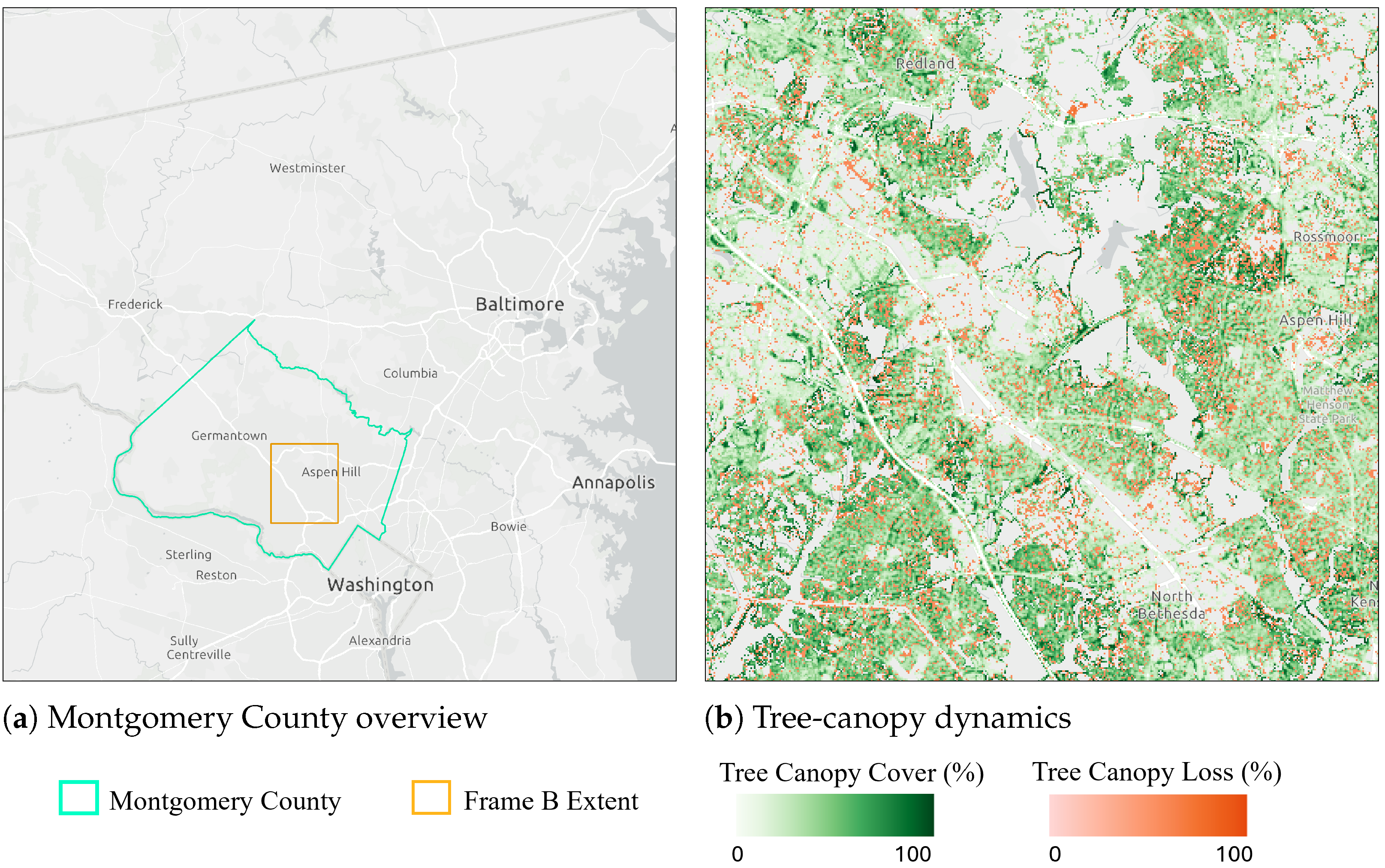
Figure 6.
Nonforest tree-canopy cover and canopy loss (2013–2016) in Montgomery County. (a) County outline (cyan) with the zoom frame for panel (b) in orange. (b) Detail showing tree-canopy cover (green gradient, 0–100%) and gross canopy loss (orange gradient, 0–100%) at 30 m resolution. The legend applies to both panels. Service Layer Credits: City of Rockville, MD, MNCPPC, VGIN, Esri, TomTom, Garmin, SafeGraph, GeoTechnologies, METI/NASA, USFS, EPA, NPS, USDA, USFWS.
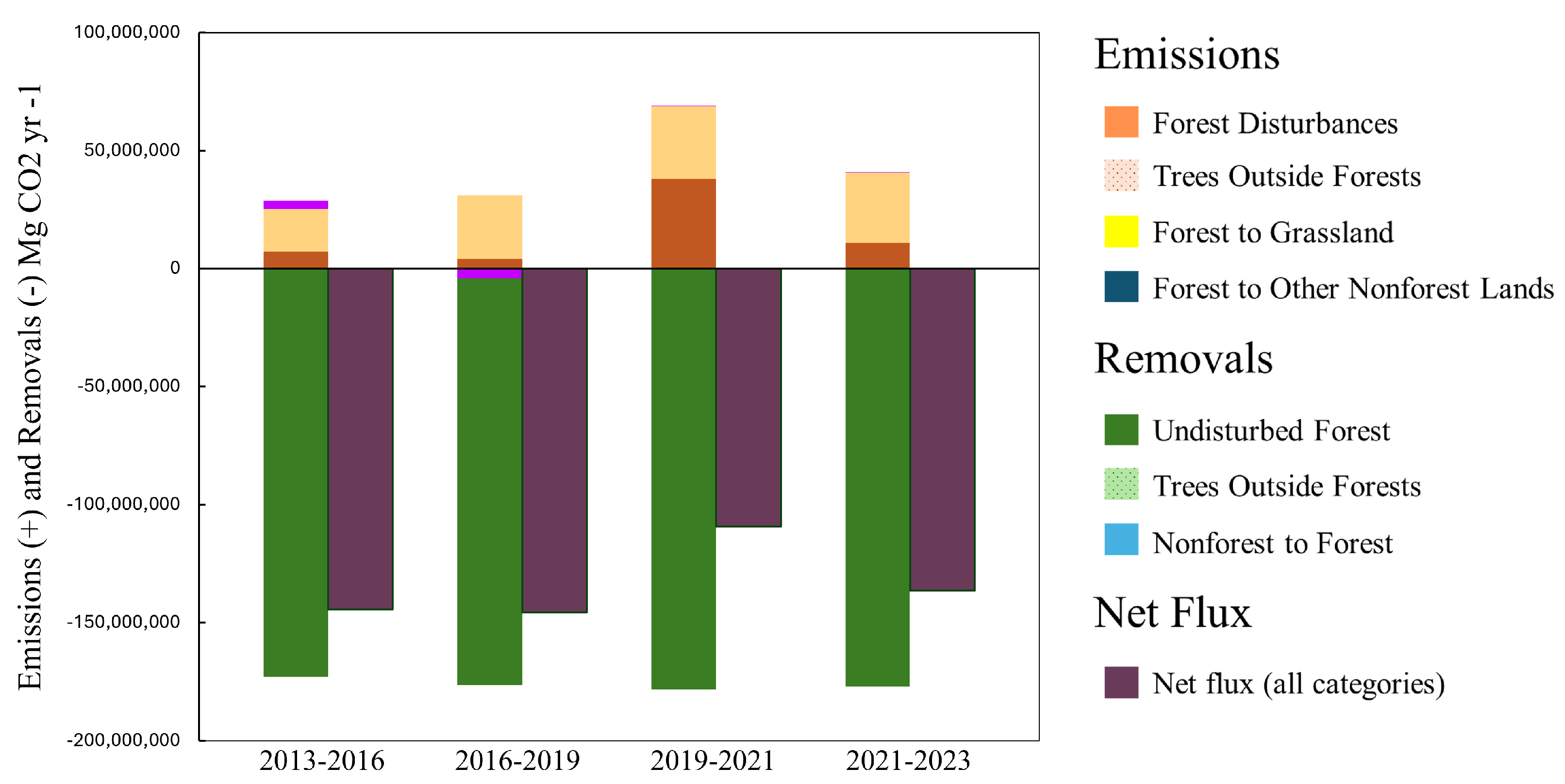
Figure 7.
Emissions from forest disturbances and removals from undisturbed forests in four successive time periods for all federally owned forests in CONUS. Stacked columns show gross emissions (positive values) and gross removals (negative values) by inventory period. Emissions result from forest disturbances and land-use transitions from forest to grassland and other nonforest land uses. Removals result from undisturbed forests and transitions from nonforest land uses to forest. Purple columns represent the overall net flux for the inventory period. All values are annual averages across the inventory period. All units in Mg CO2/year.
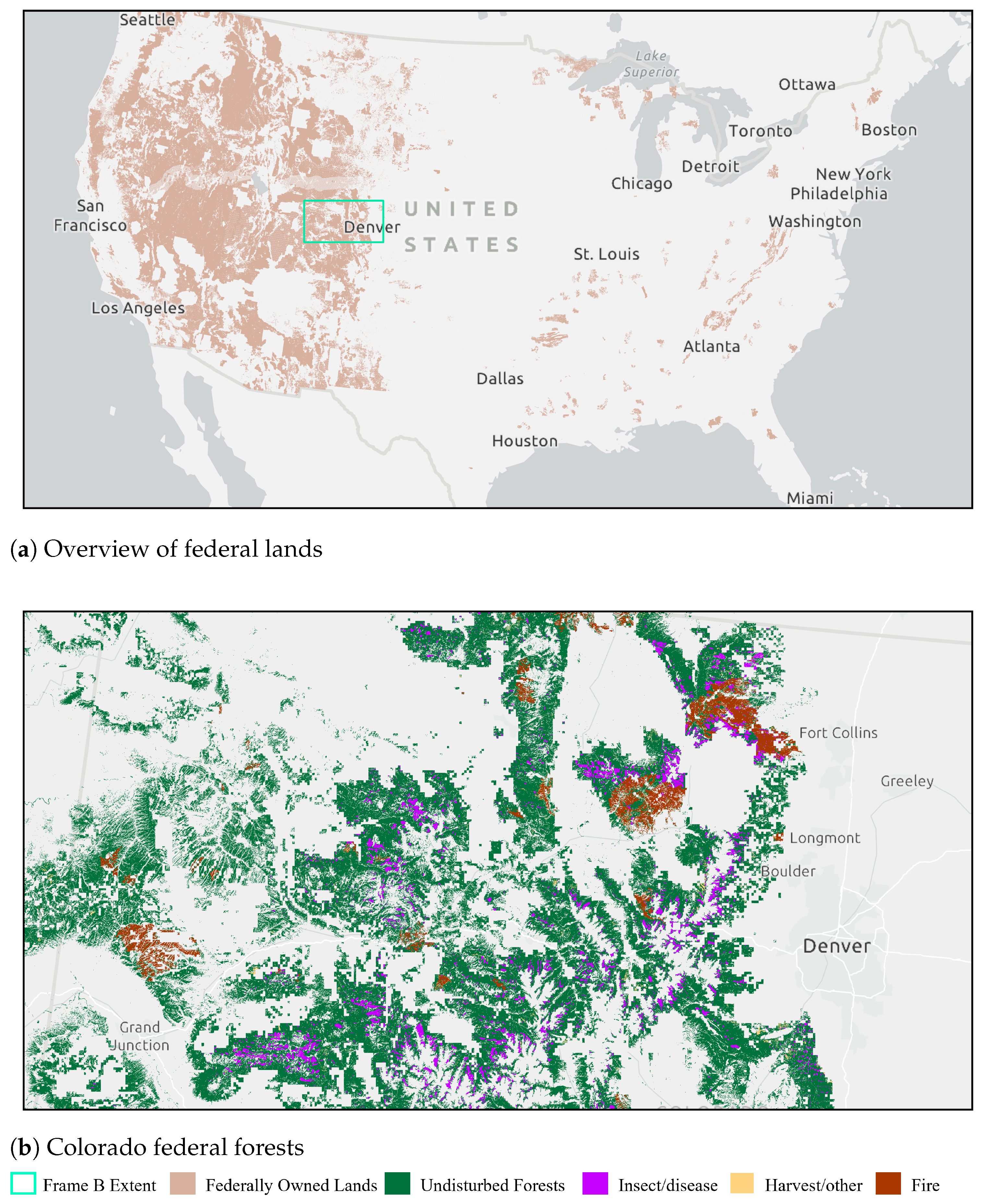
Figure 8.
Disturbance categories on federally owned forests (2013–2023). (a) Continental-US view with the zoom frame for panel (b) in cyan. (b) Detail showing undisturbed forests (green) and disturbances (fire = brown, harvest/other = orange, insect/disease = purple). The legend applies to both panels. Service Layer Credits: Esri, TomTom, Garmin, FAO, NOAA, USGS, EPA, USFWS, County of Routt, BLM, NPS.
Table 2.
Greenhouse gas inventories for four successive time periods in Jefferson County, Washington. Area units are in ha, and flux units are in Mg CO2/year. Positive values are gross emissions, and negative values are gross removals, except in the total net flux line, which is the sum or all emissions and removals per inventory period. All values are annual averages across the inventory period. Bold text denotes categories.
| | 2013–2016 | 2016–2019 | 2019–2021 | 2021–2023 |
|---|
|
Category
|
Area
|
Flux
|
Area
|
Flux
|
Area
|
Flux
|
Area
|
Flux
|
|---|
| Forest Change |
| To Forest | 4862 | −67,644 | 7181 | −102,224 | 5430 | −78,037 | 4717 | −65,397 |
| To Cropland | 0 | 0 | 0 | 0 | 0 | 0 | 0 | 0 |
| To Grassland | 5851 | 397,840 | 5677 | 533,030 | 2645 | 619,481 | 3182 | 792,061 |
| To Other | 42 | 5109 | 20 | 4477 | 40 | 13,973 | 10 | 3537 |
| To Settlement | 87 | 12,413 | 109 | 13,399 | 33 | 6397 | 42 | 9155 |
| To Wetland | 322 | 29,910 | 155 | 26,467 | 122 | 27,970 | 210 | 43,567 |
| Forest Remaining Forest |
| Fire | 477 | 41,890 | 17 | 1478 | 0 | 0 | 484 | 66,616 |
| Harvest/Other | 1325 | 271,996 | 2064 | 425,303 | 1848 | 590,065 | 1843 | 588,617 |
| Insect/Disease | 22,557 | −377,125 | 18,572 | −193,646 | 0 | 0 | 0 | 0 |
| Undisturbed | 354,328 | −4,580,890 | 356,932 | −4,635,858 | 380,079 | −4,951,419 | 381,584 | −4,973,477 |
| Trees Outside Forest |
| Maintained/gained | 16,333 | −168,885 | 15,971 | −165,141 | 15,788 | −163,251 | 14,887 | −153,933 |
| Tree-canopy loss | 558 | 65,502 | 643 | 75,471 | 484 | 85,268 | 1975 | 347,263 |
| Total Emissions | | 447,535 | | 885,979 | | 1,343,154 | | 1,850,816 |
| Total Removals | | −4,817,419 | | −4,903,223 | | −5,192,707 | | −5,192,807 |
| Net Flux | | −4,369,884 | | −4,017,244 | | −3,849,553 | | −3,341,991 |
Table 3.
Greenhouse gas inventories for four successive time periods in Montgomery County, Maryland. Area units are in ha, and flux units are in Mg CO2/year. Positive values are gross emissions, and negative values are gross removals, except in the total Net Flux line, which is the sum or all emissions and removals per inventory period. All values are annual averages across the inventory period. Bold text denotes categories.
| | 2013–2016 | 2016–2019 | 2019–2021 | 2021–2023 |
|---|
|
Category
|
Area
|
Flux
|
Area
|
Flux
|
Area
|
Flux
|
Area
|
Flux
|
|---|
| Forest Change |
| To Forest | 96 | −693 | 85 | −609 | 66 | −474 | 83 | −599 |
| To Cropland | 7 | 181 | 6 | 202 | 4 | 225 | 6 | 117 |
| To Grassland | 32 | 203 | 38 | 717 | 22 | 1444 | 28 | 1551 |
| To Other | 0 | 0 | 0 | 13 | 0 | 0 | 0 | 0 |
| To Settlement | 92 | 1,603 | 87 | 4093 | 43 | 6493 | 40 | 4655 |
| To Wetland | 10 | 115 | 17 | 157 | 18 | 255 | 6 | 144 |
| Forest Remaining Forest |
| Fire | 0 | 0 | 0 | 0 | 0 | 0 | 0 | 0 |
| Harvest/Other | 17 | 1337 | 43 | 3498 | 19 | 2665 | 15 | 2097 |
| Insect/Disease | 0 | 0 | 0 | 0 | 0 | 0 | 0 | 0 |
| Undisturbed | 38,398 | −249,973 | 38,319 | −249,456 | 38,340 | −249,592 | 38,328 | −249,520 |
| Trees Outside Forest |
| Maintained/gained | 23,430 | −303,268 | 23,477 | −303,873 | 24,062 | −311,452 | 24,079 | −311,671 |
| Tree-canopy loss | 1356 | 170,810 | 947 | 119,291 | 489 | 92,374 | 519 | 98,094 |
| Total Emissions | | 174,249 | | 127,971 | | 103,456 | | 106,658 |
| Total Removals | | −553,934 | | −553,938 | | −561,518 | | −561,790 |
| Net Flux | | −379,685 | | −425,967 | | −458,062 | | −455,132 |
Table 4.
Greenhouse gas inventories for four successive time periods in federally owned forests in the forest remaining forest category. Area units are in ha, and flux units are in Mg CO2/year. Positive values are gross emissions, and negative values are gross removals, except in the total Net Flux line, which is the sum or all emissions and removals per inventory period. All values are annual averages across the inventory period.
| | 2013–2016 | 2016–2019 | 2019–2021 | 2021–2023 |
|---|
|
Category
|
Area
|
Flux
|
Area
|
Flux
|
Area
|
Flux
|
Area
|
Flux
|
|---|
| Fire | 160,102 | 7,186,885 | 91,328 | 4,178,937 | 429,712 | 38,001,265 | 116,570 | 10,810,266 |
| Harvest/Other | 198,490 | 18,023,850 | 267,781 | 26,788,129 | 185,121 | 30,936,174 | 174,497 | 29,760,304 |
| Insect/Disease | 3,699,556 | 3,615,148 | 2,896,261 | −4,256,666 | 201 | 3,369 | 483 | 5,806 |
| Undisturbed | 46,840,576 | −173,071,224 | 47,003,598 | −172,334,863 | 48,752,295 | −178,174,491 | 48,394,716 | −177,105,604 |
| Total Emissions | | 28,825,883 | | 26,710,400 | | 68,940,808 | | 40,576,376 |
| Total Removals | | −173,071,224 | | −172,334,863 | | −178,174,491 | | −177,105,604 |
| Net Flux | | −144,245,341 | | −145,624,463 | | −109,233,683 | | −136,529,228 |
Table 5.
Comparison of LEARN and FIA area and net flux estimates. Area units are in ha, and flux units are in Mg CO2/year. Net flux is the sum or all emissions and removals per inventory period. For Jefferson County and Montgomery County, values are annual averages for the 2019–2021 period. Values exclude trees outside forests but include forests remaining forests and forest change. For federal forests, values are annual averages for the 2013–2023 period. Inventory periods were chosen to best align with FIA measurement dates. Values include forests remaining forests only.
| Case Study | LEARN Area | FIA Area | LEARN Net Flux | FIA Net Flux |
|---|
| Jefferson County | 390,712 | 384,469 | −3,875,242 | −3,966,447 |
| Montgomery County | 38,566 | 38,440 | −242,288 | −629,448 |
| Federal forests | 49,802,822 | 76,224,457 | −133,908,179 | −129,009,128 |


