From Land Conservation to Famers’ Income Growth: How Advanced Livelihoods Moderate the Income-Increasing Effect of Land Resources in an Ecological Function Area

Abstract

Balancing ecological conservation and rural livelihoods in protected areas remains a global challenge, particularly under strict land use regulations and economic development constraints. Territorial spatial planning (TSP) in an ecological function area (EFA) faces constraints such as land use restrictions, ecological redlines, and economic development limits. This study investigates how ecological land resources influence farmers’ incomes in ecological function areas (EFAs), with a focus on the moderating role of advanced livelihoods (ALI). Using an integrated Fixed-Effects–SVM–Genetic Algorithm framework, we quantify nonlinear policy-livelihood interactions and simulate multi-scenario governmental interventions (e.g., ecological investment, returning farmland to forest/RFF) across Beijing’s EFA, which can obtain the key findings as follows: (a) Ecological land resources have a significant positive effect on farmers’ incomes due to production-manner adjustment guided by governmental green strategy and corresponding TSP in an ecological restoration area of an EFA, while they have a non-significant impact in the core ecological reserve areas on account of the strict environmental protection restrictions on economic activities. (b) Differences in financial support between lower and higher economic development zones can bring about adverse impact results on farmers’ incomes in an EFA. (c) ALI significantly amplifies the positive impact of ecological land use on farmers’ incomes, demonstrating its critical role in bridging ecological and economic goals. (d) Sensitivity analysis results under RFF, targeted government investment, and ALI can maximize income gains through policy interaction from the government and farmer sides jointly. The above obtained results are beneficial to balance ecological protection and economic interests of farmers’ sustainably in an EFA.

1. Introduction

Ecological function area (EFA), designated as a critical zone for environmental protection and ecosystem service delivery, is pivotal for supporting sustainable urban development [1]. By strategically utilizing reserve space, EFAs help create integrated urban functional areas that support high quality agricultural production and enhance ecosystem services, which promotes new industries (such as the low-carbon and carbon sink industries) to support regional green development [2]. However, the EFA faces two interrelated challenges stemming from the prolonged absence of systematic territorial spatial planning (TSP). Firstly, inefficient ecosystem services (provisioning, supporting, regulating, and cultural services) and poorly circulated ecological products hinder EFAs from meeting urban populations’ multidimensional demands, undermining regional sustainability [1]. Secondly, farmers in an EFA often ignore the ecological function and corresponding benefits to depend on limited and underdeveloped livelihoods (such as supplying primary agricultural products). As a result of the EFA’s ecological conservation strategy and the simplified framework for farmers’ livelihoods, the shrinking space for economic land use can perpetuate low economic returns to ecological goods and services, which suppresses farmers’ incomes and exacerbates the urban–rural income gap [3]. Therefore, how to identify systematic TSP shaping farmers’ incomes has emerged as a critical research priority to resolve intertwined ecological and economic challenges in an EFA.

In general, territorial spatial planning (TSP) is understood to be the spatial reallocation of ecological and economic spaces based on the various land uses and characteristics, which can mediate the trade-off between economic growth and environmental protection [4]. Previous studies highlight that governments utilize TSP to optimize the ratio of ecological to economic land use, thereby enhancing regional ecological functions [5,6]. Some research demonstrates that expanding ecological land space not only safeguards environmental integrity but also transforms farmers’ livelihoods by providing ecological goods and services [7]. This transformation enables farmers to make the transition from traditional agricultural methods to eco-agriculture through the integration of factors of production such as capital, labor, and technology, which can generate diversified sources of income through participation in the ecological industrial chain [8]. Therefore, research on effective TSP and its corresponding policies (e.g., land consolidation, returning farmland to forests, ecological compensation mechanisms, etc.) to improve the efficiency of land use and increase farmers’ incomes has become the focus of attention of many scholars [9,10,11,12]. For instance, Cao et al. have analyzed Ziwuling’s Natural Forest Protection Plan to show that the plan’s costs were borne disproportionately by the local population: prohibitions on logging and grazing hindered livestock farming and decreased revenue [13]. Similarly, Collins et al. have argued that environmental policies often neglect economic trade-offs, inadvertently lowering local incomes [14]. Deng et al. have proposed the expansion of ecological land curtails agricultural activities while directly diminishing the land available for cultivation, which could reduce farmers’ incomes [15]. All the above research works indicated that a scientific and efficient design of TSP and corresponding strategies could change the economic interests of farmers, which would confront the risk of tensions between economic growth and ecological preservation for further sustainable development objectives.

The Sustainable Livelihoods Framework (SLF) is regarded as an effective manner in that farmers respond to government TSP, which refers to the capacity of individuals and communities to collectively mobilize resources, address challenges, enhance resilience, and protect natural resources [16]. Building on this framework, previous scholars have employed a number of methods such as livelihood capital indices, vulnerability assessments, income diversity metrics, and the entropy-weighted TOPSIS method to capture sustainable livelihood indicators through spatial differentiation of livelihood capital and natural resource distribution [17,18,19]. Meanwhile, various studies revealed the interplay between sustainable livelihoods and ecosystem services, climate change, and ecological compensation. These factors shaped sustainable livelihoods by driving income diversification, influencing economic stability, and fostering the residents’ level of participation [20,21]. Sustainable livelihoods continue to be extremely vulnerable to TSP decisions, especially in an EFA where land serves as both a primary asset and a constraint [22]. Thus, scholars have investigated TSP’s impact on sustainable livelihood strategies. For example, Willson found TSP combined with environmental protection programs could promote advanced livelihood transformation, which would prevent a resurgence of deforestation brought on by farmer economic pressures [23]. Alexander et al. demonstrated that TSP in an EFA could be grounded in community consensus, which could highlight the importance of participatory frameworks in ensuring sustainable development by striking a balance between improved farmer livelihoods and ecological conservation [24]. Fanta et al. evaluated the effects of community-based TSP in Ethiopia to find that participating households could achieve higher crop yields and agricultural incomes compared to non-participants [25]. Similarly, Xia et al. studied the role of Land Consolidation Programs (LCPs) in reducing rural poverty and showed that well-designed LCPs enhance livelihoods through increasing agricultural productivity, land registration, direct income, public welfare, and tourism-driven economic development [26]. Yet these studies seldom quantify how livelihood upgrading dynamically amplifies ecological land resources’ income-promoting effects in EFAs. We further reveal that higher levels of dynamic livelihood-upgrading enhance the positive impact of ecological land on farmers’ incomes. Thus, investigating how an EFA can successfully raise farmers’ standard of living and thereby carry out their function of raising farmers’ incomes becomes essential. Nevertheless, existing studies grounded in the SLF predominantly focus on preserving livelihood stability under external shocks, neglecting the dynamic process of livelihood upgrading through intentional capital reallocation and strategy innovation. To address this gap, we propose the concept of advanced livelihoods (ALI), which prioritizes proactive transitions from survival-oriented activities to development-driven livelihoods. Consequently, given the insufficient supply of ecosystem services and the underdeveloped livelihoods of farmers in an EFA, this study aims to integrate ALI as a critical regulator between ecological land resources and farmers’ income growth in EFA, grounded in ecological economics and policy optimization theories [27,28]. We seek to address the following gaps: (i) Quantify how ecological land expansion under TSP differentially impacts farmers’ incomes across protection-oriented and development-oriented zones. (ii) Identify whether ALI amplifies income gains through livelihood diversification, efficiency enhancement, or sustainability transitions. (iii) Determine the threshold combinations of TSP interventions and ALI-driven adaptations that maximize ecological-economic synergies. (iv) Determine how to combine fixed effects with machine learning for causal identification and policy simulation. Through policy scenario simulations, we further demonstrate ALI’s moderating role in bridging land conservation and income growth.

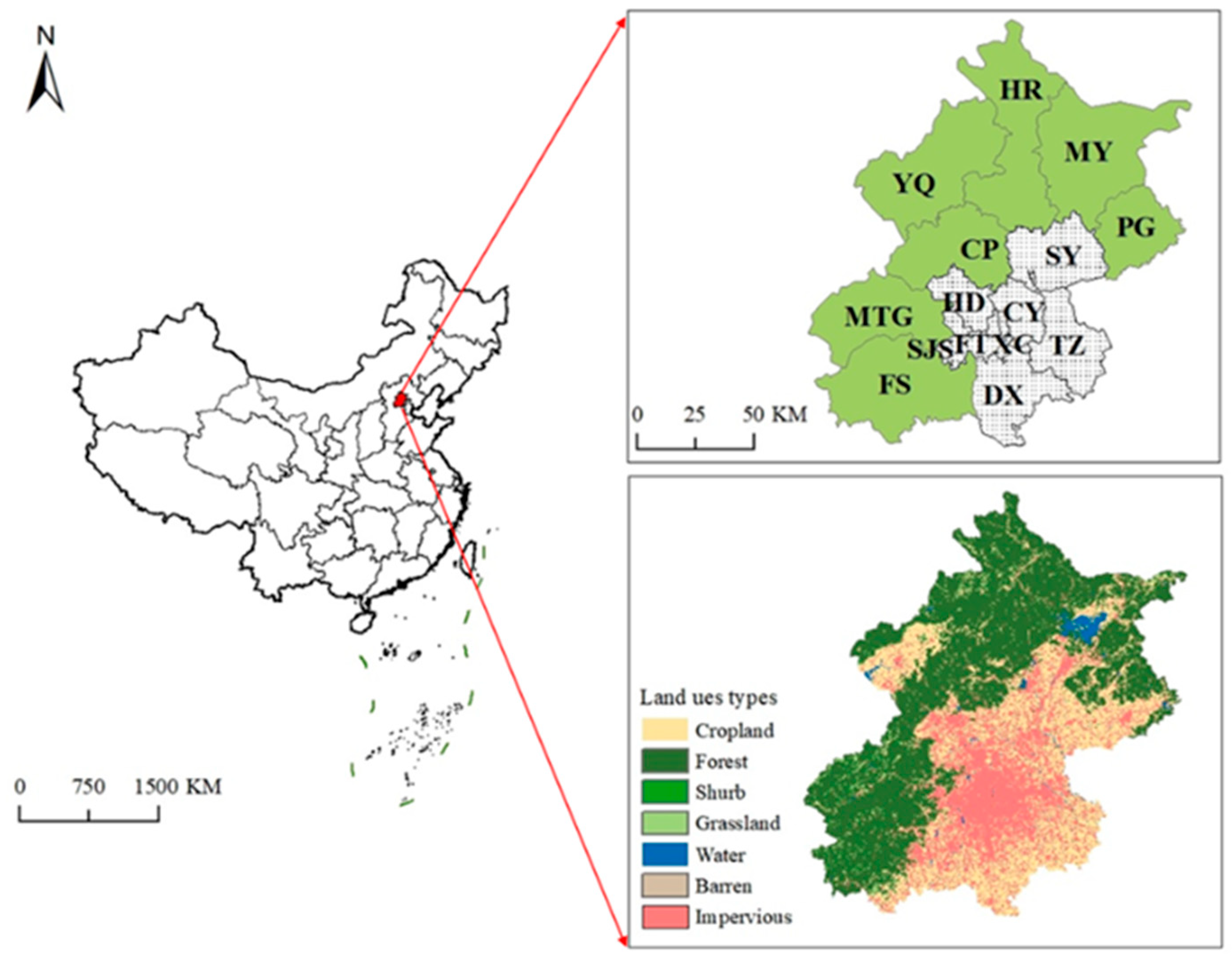
To address this gap, this study selected Beijing, China as a typical case to conduct the impact of ecological land resources on farmers’ income. Beijing’s EFA spans the areas of Mentougou (core conservation area) and Fangshan (restoration area), which is critical for the protection of water resources and biodiversity in China’s capital region. However, TSP under the ecological redline policy has constrained traditional farming development and has also shrunk economic land space, trapping farmers in low-value agricultural activities. This tension underscores the urgent need to reconcile ecological integrity with income growth through innovative livelihood transitions.

Therefore, this study constructs the ecological land resources on the farmers’ incomes (FELI) framework, which can address how government territorial spatial planning (TSP) (expansion of ecological land resources and contraction of economic land resources) in EFAs can increase farmer incomes by influencing ecosystem functioning and integrating factors of production to influence farmers’ production methods and livelihood capital choices. Advanced livelihood approaches can be considered in FELI to moderate the impact of ecological land resources on farmers’ incomes, which benefits farmers in terms of productivity and diversification of income sources. To capture the nonlinear dynamics between ecological land use, livelihood transitions, and policy interventions, we integrate advanced econometric models with machine learning techniques. This approach enables both causal inference and predictive scenario simulations. The obtained results can not only provide theoretical references for the government’s further TSP planning of EFA but also provide a better understanding of the ecological function zones from the perspective of advanced livelihoods for regional farmers. Building on this foundation, the contributions of this study are as follows: (1) The FELI framework integrates ecological economics with policy optimization, quantifying how TSP reconfigures land resources and how ALI amplifies income gains via three pathways: livelihood diversification, efficiency enhancement, and sustainability transitions. (2) Methodologically, we pioneer a causal–predictive synthesis combining econometric models with machine learning. This identifies threshold combinations of TSP interventions and ALI adaptations that maximize synergies while revealing spatial heterogeneity. (3) We empirically validate ALI’s moderating role in Beijing’s EFA—demonstrating how policy-livelihood co-adaptation operationalizes Ostrom’s governance theory [28] and China’s “Two Mountains” doctrine. By proving that high ALI levels transform land conservation from an income constraint to a development accelerator, this study offers a transferable paradigm for global EFA.

2. Theoretical Analysis

Within the institutional reconfiguration of EFA driven by land function transformation from economic use to ecological protection, a series of challenges emerges: (1) Territorial spatial planning (TSP) by governments associated with ecological land resources expanding under ecological protection policies can reduce the scale of cultivated land space (agricultural production) for farmers, which would bring about pressure on regional economic development in an EFA; (2) Various TSP strategies such as returning farmland to forest (RFF) can guide farmers’ livelihood to a sustainable way with consideration of ecological-value-oriented industries (such as ecotourism services and green agriculture) instead of traditional agriculture activities. (3) Insufficient livelihood capital (such as financial capital, human capital, natural capital, etc.) supply on account of production factors can restrict farmers’ livelihood transformation, which requires a comprehensive governmental TSP and environmental regulation in an EFA for regional ecological protection and farmers’ income improvement.

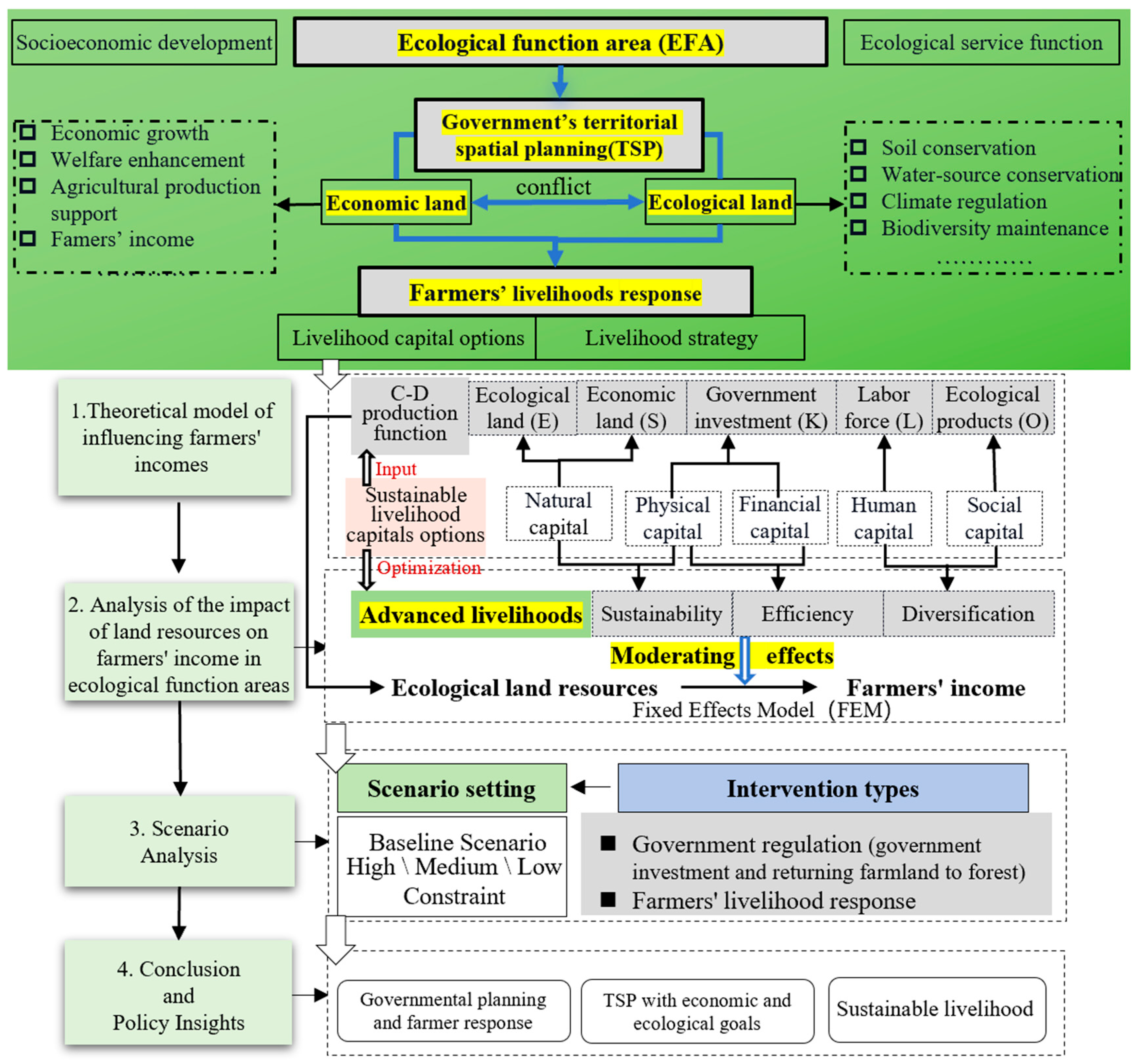
Therefore, drawing on ecosystem services valuation theory and Ostrom’s institutional analysis of commons [27,28], a theoretical analysis and empirical framework associated with the impact of ecological land resources on farmers’ incomes (FELI) in Beijing’s EFA was constructed, which reflects the complex relationship between ecological land resources and farmers’ incomes through the moderating role of advanced farmers’ livelihoods (as shown in Figure 1). The core proposition is that government-led TSP reconfigures land systems through two interdependent pathways consistent with the “Two Mountains” theory: Firstly, expanding ecological land can amplify regulating services and cultural services, thereby promoting income-generating assets. In general, the government implements differentiated allocation of economic land and ecological land through TSP, which sets up ecological function areas and promotes ecological restoration projects. On the one hand, it can enhance the regional ecological service functions by increasing ecological land resources; on the other hand, land use control changes farmers’ disposable resource endowment so that they can adjust their choice of livelihood capital and strategies, which creates a transmission chain of “government land resource planning–land use transformation–farmers’ livelihood response”. On this basis, ecological land resources can be deemed as an important ecological factor in FELI, which can be planned by the government to prompt regional economic outcomes and ecological goals. Secondly, TSP-induced land use transitions alter farmers’ access to natural capital while incentivizing the reallocation of human capital and financial capital. Under these situations, farmers deemed as “small-scale production units” can adjust their livelihood options based on various ecological and economic factors (such as ecological land resource, capital, labor, and technique) in combination with the sustainable livelihoods framework. Furthermore, by adjusting production methods and livelihood strategies, it ultimately affects farmers’ incomes. In this process, farmers’ advanced living standards play an important role as a moderating variable, which means that the higher the advanced living standards, the stronger the ability of farmers to optimize the allocation of their livelihood capital and realize the transformation of their livelihood activities so that they can more effectively transform the ecological benefits into their own income growth. Furthermore, policy scenarios are set up in intervention types of government regulation and farmers’ livelihood transformation to simulate the changes in farmers’ incomes under different circumstances in order to identify the optimal intervention pathway and explicitly test how policy can enhance ALI’s bridging role in realizing “lucid waters and lush mountains as invaluable assets”.

3. Materials and Methodology

3.1. Study Area

Beijing (115°25′–117°30′ E, 39°26′–41°03′ N) is located in the northern part of the North China Plain, at the confluence of the Yanshan Mountain Range and Taihang Mountain Range. Surrounded by mountains to the west, north, and northeast, it has a total area of 16,410.54 km² and 16 districts, with a resident population of 21.89 million (Figure 2). According to the main data bulletin of the third National Land Survey, the area of economic land (arable land and garden land) in Beijing is 2198.22 km², and the area of ecological land (woodland and grassland) is 9820.89 km². Ecological land is not only the green barrier of regional environmental sustainable development but also the key carrier of the farmers’ livelihood transformation. Under the Beijing–Tianjin–Hebei coordinated development strategy, Beijing faces the dual pressure of economic development and ecological demand enhancement. Therefore, it is important to balance the relationship between economic development and ecological protection. Beijing has delineated ecological functional areas (including Mentougou, Pinggu, Huairou, Miyun, Yanqing, Changping, and Fangshan districts) and constructed a multi-level network of ecological functional areas (EFAs) to ensure regional ecological security, optimize the spatial distribution of land, and promote the coordinated development of urban and rural areas. These areas are Beijing’s ecological barriers, water source protection zones, and “big oxygen bar” and are key areas for ensuring the sustainable development of the capital, with a variety of land use types such as woodland, cultivated land, and water bodies (as shown in Figure 2).

3.2. Method

The model development of the hybrid fixed-effects regression model–support vector machine regression coupling genetic algorithm (FSG) method includes the following aspects. First, the relationship between factor inputs (such as ecological land resources, economic land resources, financial support, and labor input) and economic/ecological outcome can be conducted by extended C-D production function. Various production materials and ecological factors can be regarded as important livelihood capitals to support farmers’ livelihood strategies. Under this situation, the effect of ecological land on farmers’ income was examined using a fixed-effect model. Second, the livelihood advanced index system is constructed in terms of efficiency, sustainability, and diversification and is tested for its role between land resources and farmers’ incomes using the moderating effect. Finally, policy scenarios were built from two aspects (government regulation and farmers’ livelihood transformation) to simulate the changes in farmers’ income under different circumstances. Moreover, policy recommendations are made from ecological investment, ecological compensation, and ecological product perspectives.

3.2.1. Analysis of the Impact of Ecological Land Resources on Farmers’ Income in Ecological Function Areas

In general, the government optimizes the spatial distribution of land resources and the functional structure of land use through TSP. As an important production factor, land resources can be not only the material basis for the functioning of the labor and capital factors, but their area, quality, and use can also directly affect economic output [29]. Therefore, based on the traditional C-D production function that contains various input factors (e.g., labor and capital), land resources can be introduced into the model as a production factor independent of labor and capital to quantitatively measure its impact on economic output [30,31]. The C-D production function with the addition of the land factor can be expressed as:

$$y=A{L}^{\delta }{GI}^{\gamma }{R}^{\omega }$$

(1)

where $y$ denotes the output, $L$ denotes labor input, $GI$ denotes government investment [32], $R$ denotes land resources, $\alpha$ denotes the output elasticity of labor, $\beta$ denotes the output elasticity of government investment, $\omega$ denotes the output elasticity of land resources, and $A$ is a structural parameter.

However, the excessive exploitation of land resources can lead to ecological problems such as land degradation, soil erosion, and the loss of biodiversity. The government balances economic development and ecological protection through the establishment of ecological functional areas and the implementation of ecological restoration while restricting land development in order to increase ecological land. Ecological land not only provides environmental security but also participates in economic production through ecological products and services. However, the traditional C-D production function ignores the contribution of ecological factors and underestimates the economic value of ecological protection [33,34]. Therefore, based on the general principle of the C-D production function, taking ecological land as an ecological factor, the C-D production function is expanded to study the impact of ecological factor input on economic output. The extended C-D production function model is expressed as follows:

$$FI2=A{LL}^{\alpha }{NL}^{\beta }{GI}^{\gamma }$$

(2)

where $FI2$ denotes farmers’ income, $LL$ denotes ecological factors (ecological land resources), $\alpha$ denotes the output elasticity of ecological land resources, $NL$ denotes economic land resources, and $\beta$ denotes the output elasticity of economic land. The extended C-D model can reveal the marginal contributions of multiple factors to economic growth and assist decision-makers in balancing the relationship between development and protection in the allocation of land resources, which further promotes the balanced development of the regional economy and ecology.

Under these situations, farmers deemed as “small-scale production units” can adjust their livelihood options based on various ecological and economic factors (such as ecological land resource, capital, labor, and technique) to adapt ecological function conservation and economic benefits in an EFA. Based on the sustainable livelihoods framework, livelihood capitals are the core and foundation and farmers can utilize rights, capital, and appropriate livelihood strategies to enhance their livelihoods in risky environments affected by markets, institutional policies, and natural factors [35]. Specifically, farmers use land resources to develop eco-agriculture, the forest economy, etc., which transforms traditional arable land into natural capital that provides ecological services such as water conservation and biodiversity protection. Farmers enhance the labor value through skills training, which extends the human capital from single farming to diversified eco-industries; farmers use government investment in infrastructure and subsidy policies to develop eco-cooperatives, introduce low-carbon technology and equipment, etc., which transforms financial support into physical and financial capital for sustainable operation. Eventually, a virtuous cycle of “ecological protection–industrial value added–feeding people’s livelihood” will be formed. Through the combination of this capital, farmers can obtain economic benefits, which are farmers’ incomes. The natural logarithm of the area on both sides of the equation is expressed as:

$$lnFI2=lnA+\alpha lnLL+\beta lnNL+\gamma lnGI+\epsilon$$

(3)

where $lnFI2$ denotes farmers’ income, $lnLL$ denotes ecological land resources (regarded as natural capital), $\alpha$ denotes the output elasticity of ecological land resources, $lnNL$ denotes economic land resources (regarded as natural capital), $\beta$ denotes the output elasticity of economic land resources), $lnGI$ denotes government investment (regarded as physical capital and financial capital), $\gamma$ denotes the output elasticity of ecological land resources, and $\epsilon$ denotes the random error term.

Then, to analyze the impact of ecological land resources on farmers’ income in EFAs, the relationship between the two is explored using fixed effects. Meanwhile, the chemical fertilizer application rate (CA), service sector income (ms), and share of primary sector value added (cz) were selected as control variables [36,37,38]. Specifically, fertilizer application rate (CA) is a core indicator of agricultural production inputs, which affects farmers’ income by influencing the yield and cost of agricultural products. Fertilizer reduction in ecological land use is a key measure for environmentally friendly agriculture; service sector income (ms) reflects the level of development of non-farm industries (e.g., ecotourism, recreational services), which may affect the structure of farmers’ income through the channel of industrial diversification; share of primary sector value added (cz) reflects the degree of dependence of the regional economy on agriculture; and ecological land use may affect this ratio through changes in agricultural practices (e.g., returning farmland to forests, ecological compensation), which needs to be controlled to distinguish the direct correlation between structural transformation of agriculture and farmers’ incomes. The model is set as follows:

$${lnFI2}_{it}={\alpha }_i+{\beta }_{1}ln{LL}_{it}+{\beta }_2{lnGI}_{it}+{\beta }_3{lnCA}_{it}+{\beta }_4{lnms}_{it}+{\beta }_5{lncz}_{it}+{\epsilon }_{it}$$

(4)

where $i$ denotes the region; $t$ denotes the year; ${\alpha }_i$ denotes the fixed effect of the ith region, which is independent of the year; ${lnFI2}_{it}$ denotes the farmer’s income of region $i$ in year $t$; $ln{LL}_{it}$ denotes the ecological land of region $i$ in year $t$; ${lnGI}_{it}$ denotes the government investment of region $i$ in year $t$; ${lnCA}_{it}$ denotes the fertilizer application of region $i$ in year $t$; ${lnms}_{it}$ denotes revenue from services in region $i$ in year $t$; ${lncz}_{it}$ denotes the primary industry value-added ratio in region $i$ in year $t$; ${\epsilon }_{it}$ denotes the residual.

3.2.2. Analysis of the Moderating Effect of Farmers’ Advanced Livelihood

The increase in ecological land resources provides farmers with more natural capital, but whether it can be effectively converted into income depends on the ability of farmers to utilize it (whether they can achieve transformation and upgrading of their livelihoods). Hence, an indicator system for the farmers’ advanced livelihoods (ALI) is constructed from three aspects, diversity, sustainability, and efficiency, to measure and analyze the diversity, sustainability, and efficiency of farmers’ livelihood activities (as shown in

Table 1. Advanced livelihood indicator system.

Goal Level	Guideline Level	Indicator Level	Units	Max	Min	sd	Indicator Properties
Efficiency	Industrial Efficiency	Value added of primary production/value added of secondary and tertiary production	-	0.13467466	0.004836674	0.032405829	−
		Gross power of agricultural machinery	(million kilowatts)	24.3	0.79235	6.492777332	+
	Agricultural productivity	Ratio of gross agricultural output/number of agricultural laborers	(1 × 109 RMB)/(1 × 104 persons)	12.65381667	2.890586241	1.848917142	+
		Gross agricultural output/cultivated land resources areas	(1 × 105 RMB)/(ha)	10.22780477	1.023152542	1.833359333	+
Sustainability	Ecologically sustainable	Annual average concentration of NO2 and SO2	(ug/m3)	93.1	17	17.42634996	−
		Sewage treatment capacity	(million cubic meters)	12,972.44	1038.3	3245.346006	+
		Amount of domestic waste disposed of in an environmentally sound manner	(million tons)	87.84886	5.3	20.72111619	+
	Infrastructure sustainability	Rural electricity consumption	(million kilowatt hours)	93,013.5	9405.6	22,302.53405	+
		Number of health institutions	(one unit)	1208	247	305.667127	+
Diversification	Diversification of livelihoods	Number of individual enterprises in rural townships	(unit)	33,434	1757	6727.541415	+
		Percentage of value added in the three sectors	-	3.322558561	0.591264105	0.729545861	+
	Diversification of services	Gross income from folkloric tourism	(1 × 104 RMB)	43,937.36	3911.34	10,488.92087	+
		Number of agro-tourism parks	(unit)	242.00	31.00	61.58108156	+

) [39,40,41]. It includes the extension of the agricultural industry chain from traditional agricultural production to higher value-added agricultural products (e.g., processing of agricultural products, branding, etc.) and the transfer from agriculture to non-agricultural industries (e.g., services, manufacturing, etc.), which results in an increase in income and an improvement in the quality of life. The traditional sustainable livelihood framework focuses on capital accumulation and diversification strategies to cope with poverty and ecological pressures through the combination of natural, human, social, and other static capitals but suffers from the following three problems: (i) it treats livelihood strategies as a passive tool for adapting to risks and ignores the efficiency of farmers in ecological functional zones in transforming their livelihoods through technological upgrading and industrial chain extension; (ii) it simplifies sustainability to the environmental carrying capacity threshold, without incorporating the reshaping mechanism of industrial sustainability on livelihood resilience; (iii) equating diversification with risk diversification fails to account for the dynamic nature of farmers’ livelihood structure leapfrogging by actively embedding themselves in the non-farm market through skills training. Furthermore, on the basis of the sustainable livelihoods framework, advanced livelihood is further defined as the transformation of farmers’ livelihood activities from survival to development based on the continuous accumulation of sustainable livelihood capital through the optimization of capital allocation and the upgrading of livelihood strategies. Among the three dimensions of ALI, (i) “efficiency” aims to illustrate that ecological premiums can be realized in ecological function area through technological upgrading (e.g., smart agriculture, green certification) and industrial chain extension (e.g., deep processing of agricultural products), rather than relying solely on traditional high-input agriculture. Industrial efficiency and agricultural efficiency directly quantify the economic benefits of ecological production methods [42]. Specifically, the primary industry (e.g., agriculture) has lower value added, while the secondary and tertiary industries, especially tertiary industry, have higher value added. Therefore, when the economic structure shifts from agriculture to non-agricultural industries, the overall economic efficiency increases, which is due to the fact that non-agricultural industries may create more value with the same inputs. (ii) “Sustainability” indicators ensure that farmers can enjoy long-term ecological dividends rather than short-term or one-time gains [43]. Specifically, environmental quality indicators build the material basis of livelihood sustainability and risk buffering mechanisms by acting directly on the core elements of farmers’ productive lives. Firstly, improvements in air quality such as the decline in NO₂ and SO₂ concentrations directly reduce the incidence of respiratory diseases among farmers, thus reducing the risk of poverty due to disease. At the same time, it improves the ability to supply labor time, forming the transformation of health capital into livelihood capital. Secondly, “sewage treatment capacity” and “amount of domestic waste disposed of in an environmentally sound manner” strengthen the system of prevention and control of agricultural water and soil pollution to avoid the accumulation of pollutants such as heavy metals and pathogens through the food chain. This not only ensures the quality and safety of agricultural products in order to maintain market competitiveness but also reduces the ineffective loss of agricultural production inputs, which creates a positive cycle of “environment–production–income”. Thirdly, the quality of the clean environment, as a fundamental element of the ecological service industry, has directly expanded farmers’ non-farm income channels and transformed livelihood strategies from “resource-consuming” to “environmentally friendly” and otherwise stabilizing the supply of electricity to guarantee eco-friendly production activities (agricultural mechanization, processing of agricultural products) and reducing fossil energy dependence. “Number of health institutions” reflects the preservation of human capital and social resilience. Adequate health resources reduce the loss of labor due to disease by reducing the risk of livelihood disruption, thus ensuring intergenerational sustainability of livelihood strategies. (iii) Ecological function areas often face restrictions on industrial access, and the “diversification” indicator verifies whether the ecological–industrial integration model actually broadens livelihood options [44].

Indicator weights and composite scores were calculated using the entropy weighting method. The data were first standardized and the formula was expressed as follows:

Positive indicator

$$y_{ij}={\displaystyle \frac{x_{ij}-x_{min·j}}{x_{max·j}-x_{min·j}}}$$

(5)

Negative indicators

$$y_{ij}={\displaystyle \frac{{x_{max·j}-x}_{ij}}{x_{max·j}-x_{min·j}}}$$

(6)

Indicator weights were calculated as follows:

$$p_{ij}=y_{ij}/\sum _{i=1}^n{y}_{ij}$$

(7)

Indicator information entropy values are expressed as $e_i=-{\displaystyle \frac{1}{ln\left(n\right)}}\sum p_{ij}ln(p_{ij})$. n is the number of samples. 0 ≤${ e}_i$≤ 1. Coefficients of variation are expressed as $d_i=1-e_i$. Indicator weights are expressed as $w_j={\displaystyle \frac{d_j}{\sum _j{d}_j}}$. The final calculated composite score is $ALI=\sum y_{ij}\times w_j$.

When the level of ALI is higher, it indicates that farmers have sustainable livelihood capabilities and diversified livelihood strategies, which is conducive to improving their utilization efficiency of ecological resources and value transformation capabilities, broadening income channels, and enhancing risk resistance capabilities [45]. Therefore, the higher the level of advanced livelihoods, the more farmers will be able to break through the limitations of crude resource utilization and fully release the potential of ecological land for income generation. Conversely, it may lead to the idleness or inefficient development of ecological resources, where the effect of increasing income will be limited. To explore the role played by advanced livelihood in the relationship between ecological land resources and farmers’ incomes, empirical tests are conducted by constructing a moderating effect model. The advanced livelihood index was selected as the moderating variable. The model is constructed by adding the cross-multiplier terms of ecological land resources and the advanced livelihood index to the baseline model. If the coefficient of the cross-multiplier term is significant, it means there is a moderating effect, otherwise there is no moderating effect. The model is set up as follows:

$${lnFI2}_{it}={\alpha }_i+{\beta }_{1}ln{LL}_{it}+{\beta }_2{ALI}_{it}+{\beta }_{3}ln{LL}_{it}\times {ALI}_{it}+{\beta }_5{control}_{it}+{\epsilon }_{it}$$

(8)

where $i$ denotes the region; $t$ denotes year; ${lnFI2}_{it}$ denotes the farmer’s income of region $i$ in year $t$; $ln{LL}_{it}$ denotes the ecological land resources of region $i$ in year $t$; ${ALI}_{it}$ denotes the livelihood advancement index of region $i$ in year $t$; ${\alpha }_i$ denotes the fixed effect of region $i$, which is unaffected by the year; ${control}_{it}$ denotes the control variable; ${\epsilon }_{it}$ denotes the residuals.

3.2.3. Hybrid Governmental Regulation and Farmers’ Livelihood Scenario Simulation Based on GA-SVR Method

Under the government’s environmental protection policy enforcement, farmers make livelihood strategy choices in an EFA, which affects the farmers’ incomes. It covers multiple dimensions of environmental protection and livelihood protection activities (involving multiple industries and sectors), whose implementation pathways are characterized by multidimensional heterogeneity. As the convergence of government policies and farmers’ livelihood options differ significantly in terms of goal orientation, action scale, and implementation mechanism, the result is policy interactions that may have complex non-linear correlation effects. However, traditional linear models have difficulty resolving such cross-scale coupling relationships. Therefore, support vector machine regression (SVR) can be used to black-box predict farmers’ income under the influence of multiple dimensions (government strategies and farmers’ livelihood options) by utilizing its better fault-tolerance and generalization ability [46]. Meanwhile, the genetic algorithm achieves global optimization of SVR hyperparameters through biological evolutionary mechanisms. Therefore, the GA-SVR model provides a more scientific approach for farmers’ income under government RFF and investment policies leading to farmers’ livelihood advancements, which can deal with the coupling effect of multiple uncertainties in farmers’ income through its hybrid intelligent algorithmic architecture effectively. By discovering the relationship between independent variables and dependent variables, it maps the data set with a nonlinear regression relationship in low-dimensional space to high-dimensional space and then transforms it into a linear regression relationship, which can be understood as

$$f\left(x\right)=w^T\phi \left(x\right)+b$$

(9)

where $w$ denotes the weight vector, $\phi \left(x\right)$ denotes the mapping function, $b$ denotes the bias. Under the condition that the constraint condition can be realized, the optimal $w$ and $b$ are found by optimization, and the optimization problem is obtained as follows:

$$\begin{gathered} min{\displaystyle \frac{1}{2}}{w}^{T}w, \\ s.t. y_i-w^T\phi \left(x_i\right)-b\le \epsilon \\ {w}^T\phi \left(x_i\right)+b-y_i\le \epsilon \\ i=1,2,\cdots ,n \end{gathered}$$

(10)

Due to the existence of outliers, the constraints in Formula (6) cannot be realized. Therefore, the relaxation variable is further introduced to transform the problem into

$$\begin{gathered} min{\displaystyle \frac{1}{2}}{w}^{T}w+C\sum _{i=1}^n\left({\xi }_i+{\xi }_i^{*}\right), \\ s.t. y_i-w^T\phi \left(x_i\right)-b\le \epsilon +{\xi }_i \\ {w}^T\phi \left(x_i\right)+b-y_i\le \epsilon +{\xi }_i^{*} \\ {\xi }_i,{\xi }_i^{*}\ge 0,i=1,2,\cdots ,n. \end{gathered}$$

(11)

By introducing Lagrange multipliers, Formula (11) is transformed into

$$\begin{gathered} min{\displaystyle \frac{1}{2}}\sum _{i=1}^n\sum _{j=1}^n{(a}_i-a_i^{*})(a_j-a_j^{*})K\left(x_i,x_j\right)+\epsilon \sum _{i=1}^n\left(a_i+a_i^{*}\right)-\sum _{i=1}^n\left(a_i-a_i^{*}\right)y_i, \\ s.t.\sum _{i=1}^n{(a}_i-a_i^{\mathrm{*}})=0,a_i,a_i^{\mathrm{*}}ϵ[0,C] \end{gathered}$$

(12)

where $a_i,a_i^{\mathrm{*}}$ denotes Lagrange multipliers; $C$ denotes penalty factor; $\epsilon$ denotes insensitive loss function; $K\left(x_i,x_j\right)$ denotes kernel function. The commonly used kernel functions include polynomial, Gaussian, and radial basis functions. Because the radial basis function has the advantages of few parameters and a wide convergence domain, this paper uses the radial basis kernel function in the support vector machine regression model. The expression is

$$k\left(x_i,x_j\right)=e^{{-\gamma ||x_i-x_j||}^2}$$

(13)

where $\gamma >0$ is the kernel function of the radial basis function.

Furthermore, the introduction of a genetic algorithm for optimization, which simulates the natural selection mechanism and searches for parameter combinations globally can find the optimal solution to minimize the prediction error in the multidimensional parameter space and guide the model to pay more attention to the distribution characteristics of the core data through the design of a fitness function to significantly enhance the robustness of the SVR in the prediction of farmer’s income. The genetic algorithm was first proposed by Holland et al. in 1975 and is mainly used to simulate natural gene mutation, reproduction, chromosome crossover, and so on [47]. It retains a set of candidate solutions through each iteration and then selects the individuals with better fitness from these candidate solutions according to the utility function. According to the genetic operator, new candidate groups are generated after selection, crossover, and mutation, and finally the convergence index is obtained. The genetic algorithm has global search ability and reduces the problem of falling into a local optimal solution. It is widely used to solve optimization problems.

The steps of the support vector machine regression model based on the genetic algorithm are as follows. Firstly, the relevant parameters of the genetic algorithm are set, and the penalty function and the gamma of support vector machine regression model are binary coded to generate the initial population. The randomly generated data is input into the support vector machine regression model, and MAE is used as the objective function. After crossover, mutation, selection, and other operations, it is judged whether the output condition is satisfied. Otherwise, crossover, mutation, selection, and other operations continue. Finally, the results are input into the support vector machine regression model to obtain the optimal parameter model for the prediction of the urban–rural income gap. The flowchart is shown in Figure 3.

Finally, the simulation model of farmers’ income under multidimensional policies (government regulation and farmers’ livelihood transformation) was constructed based on the GA-SVR model. Specifically, different scenarios (as shown in Section 4.3) were set up by combining different levels of government regulation and farmers’ livelihood transformation, and the GA-SVR model was trained to simulate and predict farmers’ incomes under different scenarios, where the input is the value of the combined scenario setting (as shown in Section 4.3) and the output is the farmers’ income.

4. Result and Discussion

The delineation of Beijing’s ecological functional areas follows the “Regulations on Ecological Protection and Green Development of Beijing’s Ecological Cultivation Areas”. Based on the layout of Beijing’s urban master plan, the entire area of the five districts of Mentougou, Pinggu, Huairou, Miyun, and Yanqing and the mountainous areas of Fangshan and Changping are included in the ecological conservation area, which covers a total area of 11,300 square kilometers, 68 percent of the city’s area. The region faces various challenges as follows: (1) the vulnerability of the ecosystem is outstanding. The high proportion of planted forests has led to low carbon sink capacity, such as Yanqing District, where the forest unit volume is only 63% of the national average; (2) people’s livelihoods are lagging behind. The per capita disposable income of rural residents in the five districts is 18% lower than that of the city, and 70% of the low-income villages are concentrated in the region; (3) the ecological value of the conversion mechanism is missing. Existing compensation standards for public welfare forests are insufficient to cover the cost of care, while market-based compensation such as carbon trading is still in the exploratory stage. Therefore, the seven districts (Mentougou District, Fangshan District, Changping District, Huairou District, Pinggu District, Miyun District, and Yanqing District) of Beijing were selected as the research object. The variables are selected as follows.

The explanatory variable is farmers’ income (FI2), which is measured using rural per capita income, and the data were logarithmized to eliminate heteroskedasticity and denoted as lnFI2. The explanatory variable is the area of ecological land resources (lnLL), which is measured using the total area of grasslands, woodlands, and water bodies, and the data were logarithmized to eliminate heteroskedasticity. Control variables include the following: (1) Government investment (lnGI). Grounded in public investment theory, government expenditure on energy conservation and environmental protection directly improves farmers’ production conditions through ecological compensation, infrastructure development, and environmental governance, thereby reducing ecological protection costs. Concurrently, it indirectly enhances income through green employment creation and technology promotion. The data were logarithmically transformed to mitigate heteroskedasticity. (2) Fertilizer application (lnCA). Based on induced technological change theory, chemical fertilizer inputs increase agricultural income by enhancing land productivity. However, excessive application may lead to environmental degradation, creating a trade-off with the environmental constraints of ecological land use. The data were logarithmically transformed to mitigate heteroskedasticity. (3) Revenue from services (lnms). Following the sustainable livelihoods framework, ecological land provides resource foundations for rural tourism and wellness industries through landscape value and biodiversity, directly augmenting non-agricultural income. This control variable helps distinguish between the “resource effect” and “industrial effect” of ecological land, preventing service industry revenues from obscuring the independent impact of ecological land. The data were logarithmically transformed to mitigate heteroskedasticity. (4) Primary industry value-added ratio (lncz). In accordance with industrial structure theory, the agricultural proportion reflects economic structural transformation that directly affects farmers’ income sources and efficiency. Ecological functional zones may inhibit non-agricultural development through industrial access restrictions. The logarithmic transformation of this ratio enhances sensitivity in capturing heterogeneous impacts of industrial transformation on income, specifically revealing the pathway through which ecological land affects farmers’ income via industrial development constraints.

Data from Beijing Statistical Yearbook. The study area is seven districts (Mentougou, Fangshan, Changping, Huairou, Pinggu, Miyun, and Yanqing), and the sample period is from 2013 to 2022 based on data availability. The software used for the calculations and regressions was STATA 16.0. Descriptive statistics for each variable are shown in

Table 2. Descriptive statistics.

Variables	(1)	(2)	(3)	(4)	(5)
	N	Mean	sd	Min	Max
lnFI2	70	0.191	0.650	−2.210	0.979
lnLL	70	11.59	0.450	10.71	12.04
lnGI	70	11.06	0.650	9.646	12.85
lnCA	70	8.089	1.191	4.944	9.403
lnms	70	9.558	0.684	8.272	10.69
lncz	70	0.0372	0.0324	0.00484	0.135
Number of id	7	7	7	7	7

Note: Data are 10-year (2013–2022) panel data for 7 regions.

.

4.1. Empirical Analysis of the Effects of Land Resources on Farmers’ Income in Ecological Function Areas

4.1.1. Benchmark Regression Results

Table 3. Fixed effects regression model results.

Variables	(1)	(2)
	lnFI2	lnFI2
lnLL	26.12 ***
	(8.970)
lnGI	0.110	0.0859
	(0.0964)	(0.0897)
lnCA	1.029 ***	0.979 ***
	(0.154)	(0.140)
lnms	−0.0406	−0.0922
	(0.165)	(0.159)
lncz	−3.028	−0.808
	(2.556)	(2.525)
lnNL		−9.816 ***
		(2.489)
Constant	−311.6 ***	92.25 ***
	(104.5)	(25.35)
Observations	70	70
R-squared	0.461	0.512
Number of id	7	7

Standard errors in parentheses, *** p < 0.01.

(1) shows that ecological land resources have a significant positive effect on farmers’ income due to the farmers’ production-manner adjustment guided by the governmental green strategy and corresponding TSP in an EFA. Based on the TSP of the EFA, ecotourism, forest recreation, and other new industries based on ecological land resources have emerged through green strategy guidance. Farmers would respond to the governmental strategy to adjust production manner, which is beneficial to convert ecological resources into economic value instead of selling agricultural products; meanwhile, farmers can directly earn business and labor income by participating in tourism service positions. It indicates that ecological land resources would increase farmers’ income, which is consistent with the extended C-D production function model. On the other hand, the government subsidizes farmers for ecological land designated for the protection of the ecological environment and the restriction of development, which provides farmers with a stable ecological compensation payment that becomes an important part of their income. Furthermore, the inclusion of economic land resources (arable land and garden land) (lnNL) in the regression equation (as shown in Table 3 (2)) reveals that the increase in economic land resources has a significant negative effect on farmers’ income in an EFA. The reasons are summarized as follows: first, economic land compression directly leads to the loss of contiguous land for some farmers, which makes it difficult to carry out large-scale cultivation. Meanwhile, the difficulty in sharing the cost of mechanical operations and irrigation makes the production cost per unit area increase instead of decrease; second, documents such as the “Regulations on Ecological Protection and Green Development of Beijing’s Ecological Culvert Areas” create harsh constraints on the use of pesticides and fertilizers and the selection of crop varieties; third, GlobeLand30 data analysis shows that the increase in construction land in Beijing from 2000 to 2020 has exacerbated the degradation of arable land quality, which directly restricts the efficiency of agricultural production and the added value of crops; finally, the China Natural Resources Development Report (2023) points out that the imperfections in ecological compensation and policy regulation mechanisms have led to the obstruction of agricultural productivity enhancement, exacerbating the difficulties in increasing farmers’ incomes. Particularly, the coefficient of service income is not significant, probably because the income from informal economic activities such as agro-industry and handicraft sales may not be included in the statistics, which leads to underestimation of the data; on the other hand, services such as ecotourism need to be cultivated for a long period of time in order to show economic benefits, and if the study period is relatively short (e.g., at the early stage of the project), it may not be able to capture the dynamic process of income growth.

In addition, the increase in “share of primary sector value added” may reflect only the expansion of inefficient agriculture rather than quality improvements. The positive pull effect on income is thus offset by multiple structural contradictions, manifesting a statistically negative but insignificant relationship. On the one hand, the strict restrictions on agricultural activities in ecological functional areas have compressed the space for expansion of traditional agriculture, making it difficult to realize large-scale cultivation, and increasing unit production costs have offset the benefits of increased yields. On the other hand, despite the fact that Beijing has adopted GEP-R accounting for the transformation of ecological value, the current low compensation standards and the lack of a long-term mechanism have made it difficult for farmers to obtain sufficient economic returns from ecological protection.

Thus, governmental guidance and TSP can facilitate farmers in the EFA to prefer ecological land use for higher value-added production activities and industries with lower environmental restrictions and costs, which would change farmers’ production manner and their livelihood choices.

4.1.2. Robustness Testing

To test the robustness of the model (4), two methods are used: the supplementary variable method and the lagged variable method. (1) Supplementary variable method: Variables added to the Table 3 (1)(2) test include the number of agro-tourism parks (lngy), rural electricity consumption (lnyd), and the number of township and village enterprises (lnxz). Among them, the number of agro-tourism parks (lngy) indicator directly reflects the degree of transformation of ecological land to a tourism service function, which is an important indicator to measure the ability of realizing ecological value. Therefore, it is used as a control variable to isolate the interference of tourism’s economic effects on farmers’ income. The growth of rural electricity consumption reflects the increased level of agricultural mechanization, facility-based agriculture, and rural electrification, which is a visual representation of the process of agricultural modernization. Therefore, the rural electricity consumption (lnyd) indicator can isolate the direct impact of energy consumption upgrading on income. The number of township and village enterprises (lnxz) reflects the industrial agglomeration effect, and township and village enterprises directly increase farmers’ wage income and business income by absorbing surplus rural labor and promoting the de-farming of the industrial structure.

Variables added to the Table 3 (2) test include agricultural mechanization technical efficiency (am) and number of laborers (nl). Among them, agricultural mechanization technical efficiency affects the level of intensive land use and production efficiency. Efficient mechanization can reduce labor intensity, improve crop yields and quality, and thus increase farmers’ operating income. However, over-reliance on machinery may exacerbate ecological risks, and it is important to avoid technological effects masking the impacts of economic land. The number of laborers reflects the regional population carrying capacity and the intensity of agricultural labor inputs. The abundant labor force can improve the land output rate through refined farming, but it may also lead to the overexploitation of ecological land due to population pressure, which can be used as a control variable to strip out the direct impact of the demographic dividend on income.

The result shows (as shown in

Table 4. Robustness test.

Variables	(1)	(2)	(3)	(4)
	lnFI2	L.lnFI2	lnFI2	L.lnFI2
lnLL	19.72 **	29.28 ***
	(9.546)	(9.019)
lnGI	0.188 **	0.0724	0.0896	0.0664
	(0.0921)	(0.0989)	(0.0862)	(0.0865)
lnCA	1.089 ***	1.277 ***	0.769 ***	1.231 ***
	(0.151)	(0.158)	(0.144)	(0.138)
lnms	−0.130	−0.0713	−0.0393	−0.133
	(0.180)	(0.163)	(0.148)	(0.148)
lncz	7.153 *	−5.480*	−1.696	−2.353
	(3.694)	(2.971)	(2.712)	(2.779)
lngy	−0.0952
	(0.244)
lnyd	0.682 **
	(0.272)
lnxz	−0.0773
	(0.126)
lnNL			−6.132 **	−12.49 ***
			(2.575)	(2.506)
jx			−0.0182
			(0.0150)
ldl			0.101 ***
			(0.0300)
Constant	−244.3 **	−349.4 ***	55.52 **	118.1 ***
	(111.6)	(105.1)	(26.13)	(25.39)
Observations	70	63	70	63
R-squared	0.569	0.590	0.601	0.668
Number of id	7	7	7	7

Standard errors in parentheses, *** p < 0.01, ** p < 0.05, * p < 0.1.

(1)(3)) that the explanatory variables are still significant after the addition of variables that may have been omitted, which implies that the core findings of this paper are robust. In addition, the coefficient of lncz becomes positive after adding the variables (Table 4 (1)). This is because before adding control variables, the model may have ignored variable bias due to the omission of key variables related to farmers’ income and primary sector share, which masks the true impact of the primary sector share. The addition of control variables absorbs some confounding factors and weakens the correlation between lncz and the error term, which turns the regression coefficient from negative to positive and significant. This suggests that the primary sector has a positive pull on income through technological empowerment or structural optimization under ecological constraints, and the original model underestimates its role by not controlling for endogenous disturbances.

(2) Lagged variable method: There is a time lag effect in the impact of land and control variables on farmers’ income; therefore, the regression analysis is rerun with the explanatory variables lagged by one period in the regression model. The regression results are shown in Table 4 (2)(4), and the explanatory variables are still significant after lagging for a period of time, which means that the core findings of this paper are robust. The coefficient of the lagged term is found to be significantly positive and larger than the baseline regression result, which may be related to the ‘self-reinforcing mechanism’ of ecological protection investment. Farmers may invest part of their earnings in eco-friendly technologies after increasing their income in the previous period, which further generates an income-enhancing effect.

4.1.3. Heterogeneity Analysis

(1)

Heterogeneity analysis across ecological function

The EFA of Beijing can be divided into core ecological reserve areas and ecological restoration areas. Among them, the core ecological reserve areas include Miyun District (denoted as MY), Yanqing District (denoted as YQ), and Huairou District (denoted as HR), which bear key ecological functions such as water conservation and water quality protection. The ecological restoration areas include Mentougou (denoted as MTG), Pinggu (denoted as PG), Changping (denoted as CP), and Fangshan (denoted as FS) districts. These areas are characterized by complex topography and rich biodiversity, which are important ecological barriers for Beijing and need to focus on protecting biodiversity. The results of the heterogeneity analysis show that ecological land resources in the core ecological reserve areas have a non-significant impact on farmers’ income (as shown in

Table 5. Results of regional heterogeneity analysis.

Variables	(1)	(2)
	lnFI2
lnLL	8.682	36.74 ***
	(8.752)	(11.88)
lnGI	−0.127 **	0.262 *
	(0.0503)	(0.138)
lnCA	0.320 ***	1.262 ***
	(0.0796)	(0.210)
lnms	0.0318	−0.314
	(0.0879)	(0.285)
lncz	−0.866	1.546
	(1.185)	(5.252)
Constant	−105.0	−425.5 ***
	(104.2)	(135.0)
Observations	30	40
R-squared	0.679	0.566
Number of id	3	4

Standard errors in parentheses, *** p < 0.01, ** p < 0.05, * p < 0.1.

(1)), while ecological land resources on farmers’ income in the ecological restoration area are significantly positive at the 1% level with an impact coefficient of 36.74 (as shown in Table 5 (2)). The results indicate that the development of the core ecological reserve areas has ecological protection as its top priority. The strict ecological protection measures have led to the restriction of some industrial activities that may have an impact on the ecological environment, which affects the opportunities for farmers to increase their income through industrial development. However, the ecological restoration area has focused on combining ecological restoration with industrial development while promoting ecological restoration, which has provided farmers with more channels to increase their income through the development of eco-tourism, green agriculture, and other industries.

(2)

Heterogeneity analysis across economic development

Based on the economic development within the study area, it was categorized into higher economic development zones (including FS, CP, HR, and PG) and lower economic development zones (including MTG, MY, and YQ). It was found that the effect of ecological land resources on farmers’ income within the lower economic development zones was not significant (as shown in

Table 6. Results of economic development heterogeneity analysis.

Variables	(1)	(2)
	lnFI2
lnLL	6.304	6.927 *
	(58.45)	(4.058)
lnGI	0.254	0.0501
	(0.352)	(0.0374)
lnCA	1.276 ***	0.204 *
	(0.261)	(0.119)
lnms	−0.349	−0.0250
	(0.498)	(0.0781)
lncz	−4.485	2.874 *
	(6.011)	(1.654)
Constant	−83.57	−80.85 *
	(689.0)	(46.97)
Observations	30	40
R-squared	0.566	0.362
Number of id	3	4

Standard errors in parentheses, *** p < 0.01, * p < 0.1.

(1)), while the effect of ecological land use on farmers’ income within the higher economic development zones was positively significant (as shown in Table 6 (2)). The obtained results show the following: (a) The lack of financial support and dependence on traditional agriculture in the lower economic development zones lead to an insignificant impact of ecological land use on farmers’ income in the region. The lower economic development zones may face the problem of a low economic base. These districts may lack sufficient financial support and technical inputs to effectively develop and utilize ecological land resources, thus limiting their contribution to the growth of farmers’ income. In addition, these districts may rely too much on traditional agriculture, while new industries such as eco-agriculture and green industry have not yet been fully developed, which results in the limited contribution of eco-land to farmers’ income. (b) The tertiary industry is more complete in the areas with higher economic development, which leads to the positive impact of ecological land use on farmers’ income. Higher economic development areas have a stronger economic base, which can invest more capital and technology to develop and utilize ecological land resources. By promoting the development of new industries such as eco-agriculture and green industries, they can significantly increase farmers’ income. In addition, these regions may have optimized and upgraded their industrial structure, which makes eco-agriculture, green industry and other new industries an important pillar of economic growth. Therefore, ecological land use can better serve economic development and thus promote the growth of farmers’ income.

Furthermore, government investment has not contributed to increasing farmers’ incomes. This indicates that the prioritization of ecological protection has limited the intensity of agricultural development and the choice of industries, resulting in investments focused on environmental management rather than on direct income-generating projects.

4.2. Moderating Effect Mechanism Test Based on Advanced Livelihoods

4.2.1. Heterogeneity Analysis of the Advanced Livelihood Indicator (ALI)

According to an indicator system for the farmers’ advanced livelihoods (with consideration of diversity, sustainability and efficiency) in Table 1, ALI calculations from 2013 to 2022 can be obtained in Figure 4. Among them, the legend shows the range of ALI values, and the colors indicate the different intervals of ALI values. It is due to the result of the two-way role of the government strategies and the individual farmers. On the one hand, the government introduced policies such as ecological compensation and industrial support. Both protect the economic interests of farmers sacrificed due to ecological protection and guide them to participate in ecological industries with incentives such as financial subsidies and tax concessions. On the other hand, farmers break through the traditional business model to explore new business subjects. According to market demand, take the initiative to expand the sale of ecological products and utilize e-commerce platforms and other channels to transform ecological advantages into economic benefits. Specifically, Mentougou District (MTG) has the lowest ALI level and Fangshan District (FS) has the highest ALI level. In 2013, MTG had an ALI value of 2151.3 and FS of 9414.2; in 2016, MTG had an ALI value of 2449.5 and FS of 9174.8; in 2019, MTG had an ALI value of 2540 and FS of 7391.7; and in 2022, MTG had an ALI value of 3029.3 and FS of 7553.1. The results indicate that MTG has a lower ALI due to mountainous terrain restrictions and ecological protection positioning, which limits the extension of the agricultural industry chain and the transfer to non-agricultural industries. FS is located in the southwest of Beijing (far from the city center) but has a beautiful natural environment and rich tourism resources and diversified farmers’ livelihoods. Therefore, the differences in regional positioning and functions between FS and MTG have led to large differences in the ALI.

4.2.2. Moderating Effect of Advanced Livelihoods

Table 7. Mechanism test results.

Variables	(1)
	lnFI2
lnLL	18.64 **
	(8.299)
lnLL×ALI	4.771 ***
	(1.096)
ALI	−0.000673 ***
	(0.000185)
lnGI	0.164 *
	(0.0854)
lnCA	0.937 ***
	(0.135)
lnms	−0.430 **
	(0.195)
lncz	2.797
	(2.621)
Constant	−313.5 ***
	(96.67)
Observations	70
Number of id	7
R-squared	0.606

Standard errors in parentheses, *** p < 0.01, ** p < 0.05, * p < 0.1.

shows the results of the moderating effect mechanism test, which revealed that ecological land resources are significantly positively associated with farmers’ income; the interaction term is significantly positively associated with farmers’ income; and livelihood advancement is significantly negatively associated with farmers’ income. Specifically, livelihood advancement plays a positive moderating role in the impact of ecological land use on farmers’ income. In other words, as the level of livelihood advancement increases, the promotion effect of ecological land resources on farmers’ income will be further enhanced. This is due to the fact that livelihood advancement brings about the extension of the agricultural industry chain, the development of high value-added industries such as agricultural product processing and branding, and the transfer to non-agricultural industries such as the service industry and manufacturing industry, which increases the sources and channels of farmers’ incomes.

4.3. Scenario Analysis

4.3.1. Scenario Setting

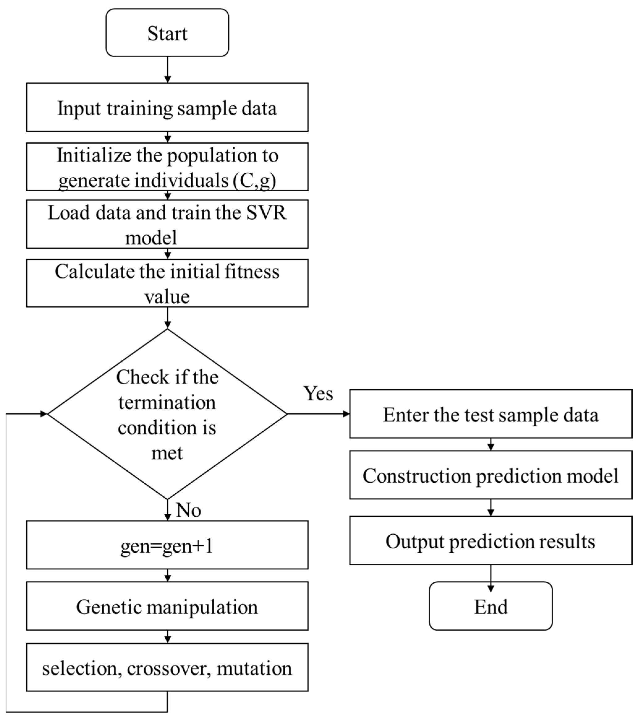
The fixed-effects model identifies the core impact pathways and moderating effects of ecological land on farmers’ incomes, in which the results of its parameter estimation (e.g., coefficients of key variables, nonlinear thresholds) provide theoretical constraint boundaries for the GA-SVR model; subsequently, the GA-SVR model takes the significant variables screened in the fixed-effects model as the core input features and optimizes the kernel function parameters and penalty factors of the support vector machine through genetic algorithms so as to enhance the prediction accuracy of complex nonlinear relationships (e.g., time-lag effects of policy shocks, multi-scenario interactions) while retaining the rigor of statistical inference. Although the two do not construct an end-to-end joint loss function, they not only avoid the limitations of linear assumptions of fixed-effects models in scenario simulation but also avoid the black-box risk of pure machine learning models, forming a closed-loop framework of “statistical inference/prediction optimization”.

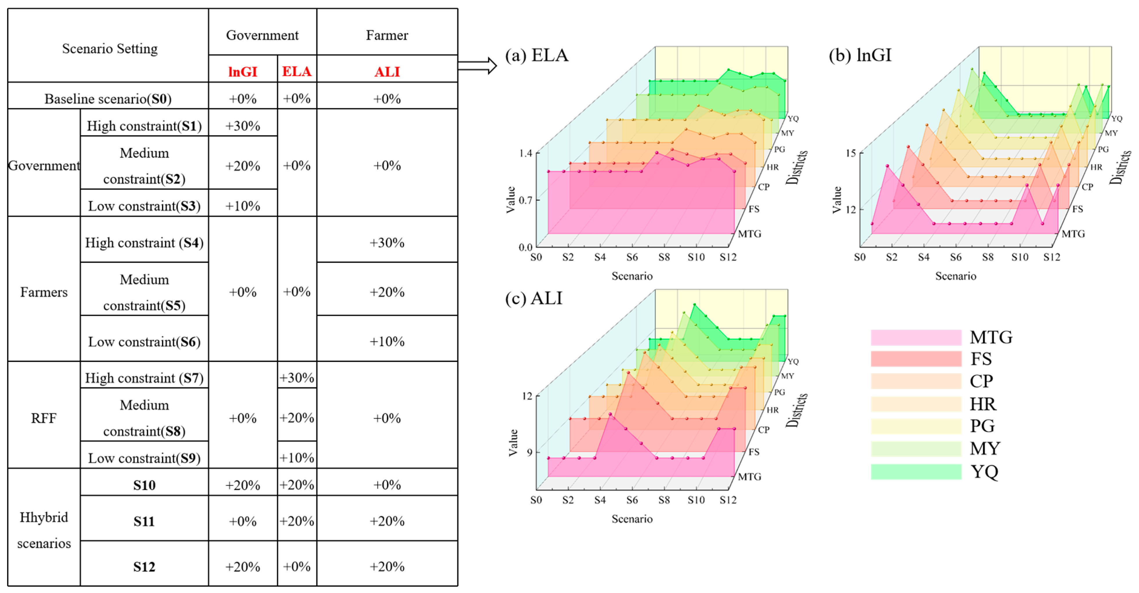
In order to reflect the land use changes under the government’s environmental protection policy enforcement, which enables farmers to make livelihood strategy choices and thus impact arm incomes, scenarios were set up to simulate farmers’ incomes in 2022 under different scenarios from both the government (returning farmland to forest (RFF) and government investment (lnGI)) and farmer (ALI) perspectives. Specifically, (1) 2022 is used as the baseline scenario to set S0. It means that the variables lnGI, ELA, and ALI are all actual values in 2022 without any adjustment. (2) From the government’s point of view, increases of 30%, 20%, and 10% are made to lnGI, whereby scenarios S1, S2, and S3 are set up. Specifically, using the Overall Plan for Major Projects for the Protection and Restoration of Nationally Important Ecosystems (2021–2035) as the policy benchmark, combined with the local matching fund linkage mechanism, the actual increase in comprehensive inputs can reach 20–30%. The scenario is therefore policy feasible. (3) From the farmer’s point of view, increases of 30%, 20%, and 10% are made to ALI, whereby scenarios S4, S5, and S6 are set up. Specifically, the target of the “New Professional Farmer Cultivation Project” in the “14th Five-Year Plan for Promoting Modernization of Agriculture and Rural Areas” is that the total number of high-quality farmers will exceed 20 million by 2025 (with an average annual growth rate of about 15 per cent). The scenario is therefore policy feasible. (4) From RFF’s point of view, 30%, 20%, and 10% increases are made to the ecological land resources area share (ELA), whereby scenarios S7, S8, S9 are set up. Specifically, based on the National Land Greening Plan (2022–2030), which proposes to complete afforestation and greening of more than 50 million mu per year during the 14th Five-Year Plan period, an increase of about 18% compared with the actual completion during the 13th Five-Year Plan period, the scenario parameters are set to match the policy intensity. Therefore, the parameters of the scenario match the strength of the policy. (5) From the hybrid scenario is (a) Scenario S10, a 20% increase in lnGI and ELA. Scenario S10 is set up according to “Beijing Municipal Opinions on Improving the Follow-up Policies for Returning Farmland to Forests”, where the policy requires the government to support the implementation of the policy of returning farmland to forests by increasing investment, including the provision of land resource transfer fees, forest maintenance fees, and agricultural subsidies, in order to promote ecological environment improvement and the increase in farmers’ incomes; (b) Scenario S11 includes a 20% increase in ELA and ALI. According to the “Beijing Municipal People’s Government’s Implementation Plan on High-Quality Promotion of Ecological Protection and Green Development in Ecological Culvert Areas in the New Era” for scenario S11, the policy proposes to strictly control ecological space and encourages rural professional cooperatives to dock with e-commerce and to actively develop e-commerce and other new business forms; (c) Scenario S12 features a 20% increase in lnGI and ALI. Scenario S12 is set according to “Several Measures on Promoting the Increase of Farmers’ Income in the City”, which proposes to promote the development of rural tourism, steadily raise the level of security for urban and rural residents, increase the support for agricultural science and technology and human resources, and guide the standardized and orderly transfer of contracted land resource management rights and other aspects (as shown in Figure 5).

4.3.2. Simulation Results Under Various Scenarios

In order to measure the prediction accuracy of the GA-SVR model, the coefficient of determination (R2), root mean square error (RMSE), and mean average error (MAE) evaluation metrics are further calculated.

Table 8. GA-SVR model performance.

	R2	RMSE	MAE
GA-SVR	0.982	0.096	0.070

shows that the model has good fitting performance and can be further used for scenario prediction.

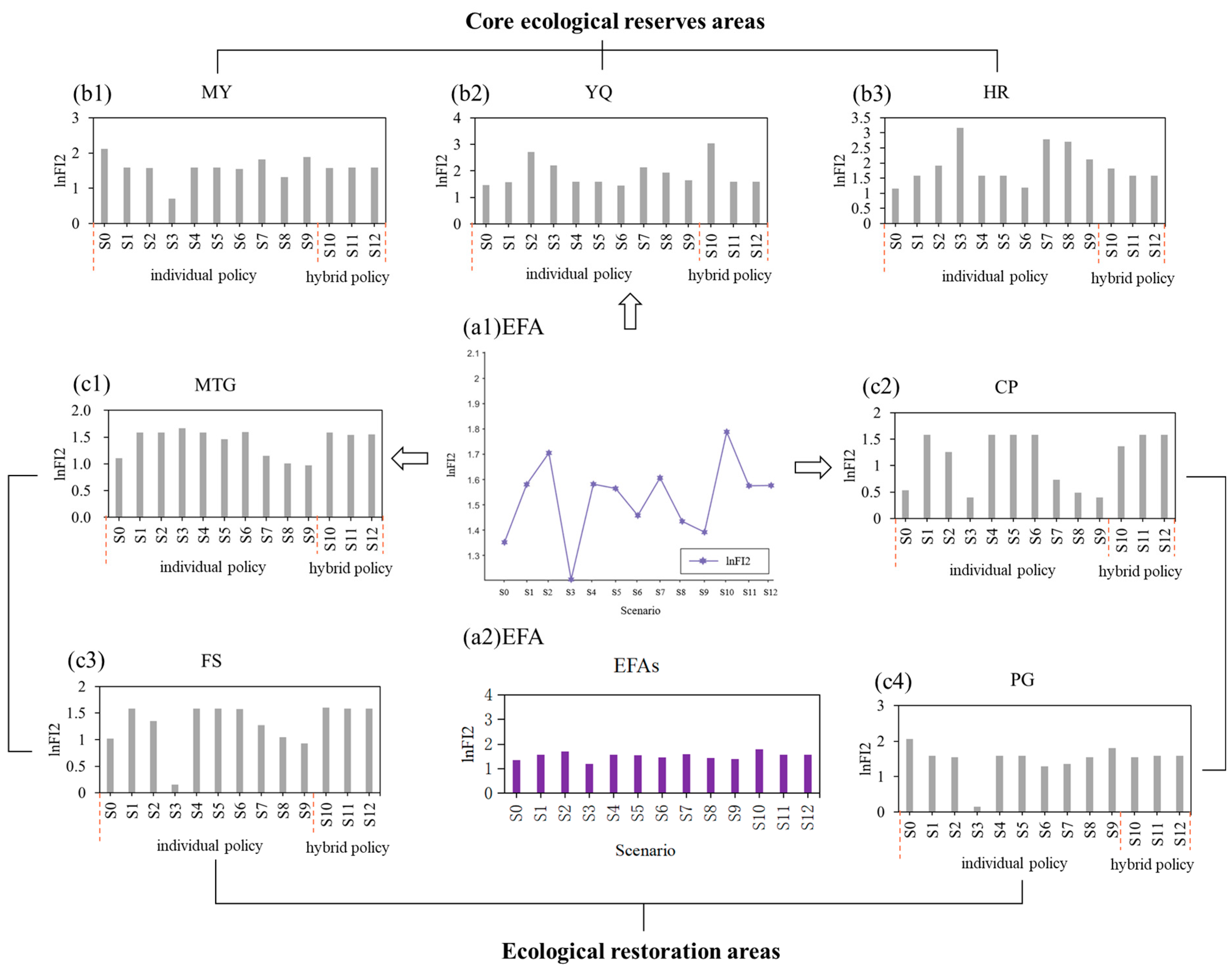
Figure 6 shows farmers’ incomes in an EFA under different scenarios (individual policy and hybrid policy) associated with government and farmer perspectives. FI2 (farmers’ income) is in RMB, but here it is logarithmized to become dimensionless and denoted as lnFI2 in order to reduce the effect of extreme values on the model. The results show that farmers’ income is highest under S10 with 1.78813554. In other words, the highest level of farmers’ income was achieved when both government investment and RFF were implemented at the same time. Specifically, MTG and HR have the highest farmers’ incomes in the S3 scenario; FS and YQ have the highest farmers’ incomes in the S10 scenario; CP has the highest farmers’ incomes in S4 and S5; and PG and MY have the highest farmers’ incomes in the S0 scenario.

Specifically,

Table 9. Percentage change compared to S0.

	MTG	CP	PG	YQ	FS	HR	MY
S1	42.99%	196.76%	−23.43%	7.89%	55.40%	36.35%	−25.04%
S2	43.28%	135.80%	−25.05%	86.04%	32.47%	64.32%	−25.35%
S3	50.34%	−25.80%	−93.20%	51.13%	−84.76%	173.14%	−66.42%
S4	42.99%	196.77%	−23.43%	8.34%	55.50%	36.36%	−25.04%
S5	32.28%	196.77%	−23.43%	8.34%	55.50%	36.36%	−25.04%
S6	44.08%	196.26%	−37.84%	−0.50%	54.41%	2.20%	−27.02%
S7	4.13%	36.63%	−34.32%	46.24%	25.71%	139.46%	−13.79%
S8	−9.23%	−8.39%	−24.88%	32.27%	3.24%	133.22%	−37.78%
S9	−11.96%	−24.72%	−12.90%	12.84%	−8.32%	82.14%	−10.99%
S10	43.13%	155.49%	−25.48%	108.49%	57.19%	56.29%	−25.25%
S11	39.01%	196.73%	−23.45%	8.33%	55.51%	36.34%	−25.04%
S12	39.81%	196.73%	−23.45%	8.33%	55.51%	36.34%	−25.04%

shows the value of income or the percent change from S0 for each area under each scenario; this indicates that different scenarios have heterogeneous impacts on different districts due to factors such as developmental orientation, economy, environment, and industrial structure.

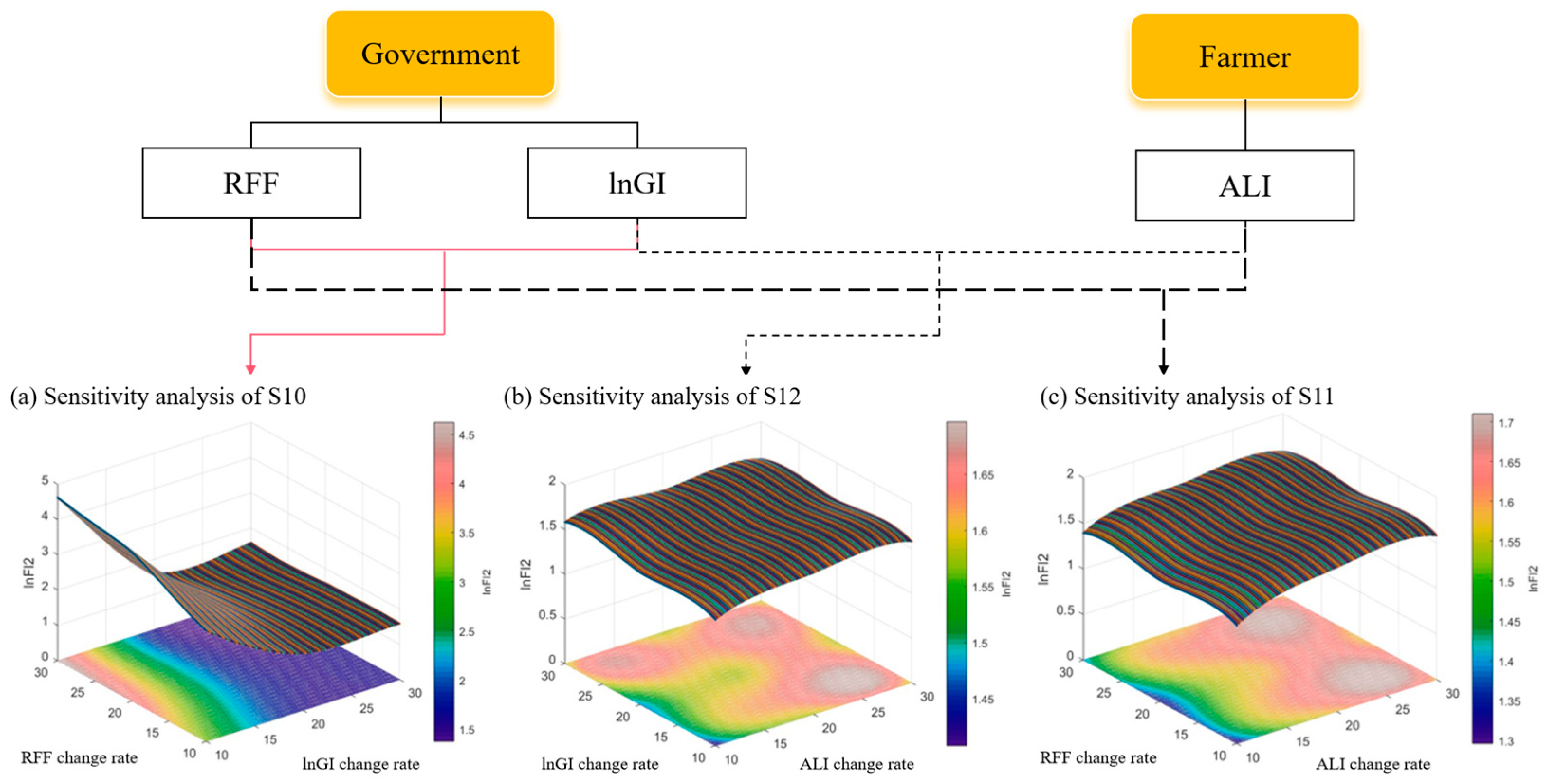
Therefore, a sensitivity analysis of farmers’ incomes was conducted for the hybrid scenarios (S10–S12) and can be obtained in Figure 7, where 10–30% growth for RFF, lnGI, and the ALI was re-entered into the model. Figure 7a shows that farmers’ income was highest under scenario S10 at a 30% increase in RFF and a 10% increase in lnGI. Figure 7b shows that farmers’ income was highest under scenario S12 at a 25% increase in ALI and 15% increase in lnGI. Figure 7c shows that farmers’ income is highest under scenario S11 at a 25% increase in RFF and 25% increase in the ALI. It indicates the following: (1) Increasing green vegetation cover and improving the ecological environment has a significant effect on enhancing farmers’ income. It indicates RFF promotes the development of eco-agriculture, improves the ecological service function and productivity of the land resources, or provides opportunities for farmers to participate in new industries such as ecotourism. (2) Government support should be moderate. Instead of over-investing, the government should focus on efficiency to ensure that funds and resources are used in a precise way to promote farmers’ income growth. (3) Upgrading the ALI is an important way to achieve the optimization of the livelihood structure and sustainable growth of farmers’ income.

4.4. Discussion

Above all, to advance understanding of EFA governance and policy formulation, we ground our findings in theoretical frameworks that address critical gaps in prior studies. In contrast to Deng’s results that the expansion of ecological land not only restricts agricultural activities but also directly reduces the amount of land available for farming, which may reduce farmers’ incomes [15], this study empirically analyzes the complex impact mechanism of ecological land on farmers’ incomes in Beijing’s EFA and introduces ALI as a moderating variable. Specifically, drawing on Ostrom’s social/ecological systems theory, which rejects simplistic panaceas, we identify the ALI as a context-adaptive moderator. And then we find that in the EFA, as the level of the ALI increases, the promotion effect of ecological land resources on farmers’ income will be further enhanced. This demonstrates how locally tailored livelihood diversification strategies, such as Beijing’s eco-tourism, convert resource constraints into sustainable income pathways. Simultaneously, the “Two Mountains” theory provides the value-realization mechanism. Unlike the findings of Cao’s study in Northwest China, which showed that the costs of environmental policies are disproportionately borne by local residents, thereby reducing farmers’ incomes [13], our evidence shows that the ALI bridges restricted land access to non-farm revenue streams, operationalizing the concept of “lucid waters and lush mountains” as invaluable assets rather than liabilities through market-based channels and cultural-ecosystem services. This study further extends the existing research by simulating policy scenarios to analyze the changes in farmers’ incomes from the perspectives of both the government and farmers. Crucially, policy effectiveness depends on leveraging the ALI’s dual role. Moreover, this study shows that the diversified income-generating channels (e.g., eco-tourism, carbon trading) in Beijing’s EFA may explain the heterogeneity of the moderating effect. As an Ostromian adaptive tool, promoting the ALI requires polycentric governance structures. For instance, participatory co-design of compensation schemes aligned with local income structures avoids omnipotent approaches and empowers communities to self-organize around resource/income synergies. As a “Two Mountains” converter, authentically utilizing the ALI’s moderating role demands policy instruments, like digital platforms connecting farmers to eco-product buyers or payments for watershed services, which explicitly translate ecological stewardship into transactional livelihood benefits.

5. Conclusions

In this study, an ecological/economic synergy analysis framework was constructed by coupling the fixed-effects model and the GA-SVR model. The fixed-effects model effectively stripped away the interference of spatial heterogeneity and clarified the causal relationship between ecological land use and farmers’ incomes, while the GA-SVR model optimized the parameters through genetic algorithms to realize the dynamic simulation of the complex nonlinear effects and multi-scenario interactions. Taking the Beijing ecological functional area as the study area, it is found that ecological land has a positive impact on farmers’ income, and its effect is significantly amplified by the advanced livelihoods (ALI) of farmers. And there is regional heterogeneity that ecological restoration zones and high-development areas have a greater impact on the growth of farmers’ income; the policy simulation shows that the simultaneous implementation of the combination strategy of returning farmland to forests and government investment can optimally balance ecological protection and rural development, which provides a scientific path for the precise implementation of policies.

The corresponding suggestions are recommended as follows: (1) Land resource utilization policies need to be diversified upon various functional positions, which should take human well-being and ecological services into account comprehensively. Heterogeneity analysis reveals that ecological land resources in ecological restoration zones and high economic development zones are more effective in increasing farmers’ income. Therefore, priority should be given to scaling up eco-agriculture practices, strengthening forestry-based industrial chains, and improving processing and marketing systems to enhance resource conversion efficiency. In high-economic development zones, promoting eco-tourism, wellness industries, and eco-industrial integration could maximize the economic potential of land resources through intensive utilization. Conversely, in core ecological reserves and low-economic development zones where ecological land exhibits limited income effects, a dynamic ecological compensation mechanism must be institutionalized. This mechanism should quantitatively assess direct conservation costs and development opportunity costs, allocating compensation funds to targeted environmental protection, education, healthcare, and livelihood enhancement programs, while establishing differentiated compensation standards proportionate to regional economic development levels. (2) Leveraging the moderating power of the ALI is critical. Therefore, regionally tailored ecological skills training programs should be implemented to cultivate interdisciplinary talents proficient in modern agro-technologies, thereby optimizing labor/ecological resource matching efficiency. A tiered ALI-linked compensation framework ought to be designed, prioritizing fiscal transfers to low-ALI regions, and it should adopt synergistic eco-technology and industrial upgrading models to catalyze a virtuous cycle of capacity enhancement, resource optimization, and income growth. These multidimensional strategies aim to reconcile ecological preservation, economic vitality, and equitable livelihood improvements. (3) The synergistic effects of government regulation and livelihood pattern adjustment need to be considered to improve the efficiency of policies. Beijing’s EFA must create a mechanism that connects ecological protection and fiscal support, combining targeted fiscal transfer payments, ecological environment protection, and land resource governance. This strategy seeks to bring about shared ecological prosperity for the area’s farmers. Sensitivity analysis shows that farmers’ income can be maximized by extending the RFF policy by 30% and increasing government investment by 10%. Thus, it is essential to create a dynamic adjustment mechanism that, while keeping overall fiscal expenditure under control, gives priority to fiscal transfer payments to regions exhibiting both industrial growth and ecological protection.

In future research, further improvements can be made in the following aspects: (1) Measuring ecological land resources from multiple dimensions (quality of ecological land resources, diversity of ecological functions, and value of ecological services) can more accurately evaluate the impacts on farmers’ livelihoods and incomes. (2) Consider the spatial correlation and spillover effects of ecological land resources, farmers’ incomes, and livelihood advancement. Changes in ecological land resources in different regions may affect farmers’ incomes in neighboring regions through ecological corridors, markets for agricultural products, and labor mobility, while the process of livelihood advancement may also involve mutual learning and imitation among different regions. Consideration of spatial effects can lead to a fuller understanding of the relationship between variables and an accurate grasp of the mechanism of synergistic development between regions. (3) Analyzing the impact of ecological land resources on farmers’ income from a micro perspective. The study mainly analyzes the impact of ecological land resources on farmers’ incomes and the regulating effect of livelihood advancement from the macro level. Future researchers will further study the behavioral decision-making process, motivation, and constraints of farmers in the face of ecological land resource changes from a micro perspective. (4) There are problems of endogeneity due to time-varying omitted variables and potential reverse causality in the empirical tests, which will be compensated for in subsequent studies by using nonlinear methods, instrumental variable methods, etc., to compensate for the limitations of this study.