1. Introduction
As economic globalization advances, and countries enhance their specialization of industrial division, such as through global trade [
1], investment [
2], and carbon trading [
3], developed countries shift high-pollution and high-emission industries to developing countries to meet emission reduction targets [
4]. Developed countries relocate energy-intensive and high-emission manufacturing stages to developing countries through industrial transfer, leading to the formation of a global value chain (GVC) pattern characterized by “production in low-income countries and consumption in high-income countries.” Apparent carbon emission reductions in developed countries are achieved at the expense of actual carbon increases in developing countries, resulting in the phenomenon of the “pollution paradise hypothesis”. Since the 1980s, the rise of information and communication technology (ICT) has significantly contributed to the fragmentation and spatial reorganization of international production processes, thereby leading to the establishment of global value chains [
5]. Within GVCs, the specialization of labor has not only redefined global trade patterns but also modified the dynamics of carbon emissions associated with trade [
6]. However, since the 1990s there has been a pronounced and accelerating shift toward cross-border trade in intermediate goods. It means that the value added in these products is now distributed across multiple nations [
7].
According to the International Energy Agency [
8], emissions in China grew around 565 Mt in 2023, by far the largest increase globally and a continuation of China’s emissions-intensive economic growth in the post-pandemic period. Since joining the World Trade Organization in 2001, China’s rapid economic growth has been accompanied by environmental degradation and a dramatic increase in carbon emissions, exceeding one-third of the world’s total emission. At present, the production-based accounting (PBA) approach, as outlined in the United Nations Framework Convention on Climate Change (UNFCCC), is widely employed in international practices for regional carbon emission inventories. But this method has been criticized for the potential issue of carbon leakage through imports from non-Annex I to Annex I countries [
9]. China has long exhibited the characteristic of “significantly higher production-based carbon emissions compared to consumption-based emissions.” According to the Consumption-Based Carbon Emissions Research Report (2024), the gap between the two increased from 0.7 billion tons to 1.8 billion tons during the period of 1990–2019. This indicates that China has borne a substantial volume of embodied carbon emissions through its exports and remains the world’s largest net exporter of embodied carbon emissions via trade. This imbalance underscores the limitations of traditional production-based accounting systems and necessitates the incorporation of a consumption-based perspective to clarify responsibility attribution. Approximately one-third of China’s aggregate carbon emissions stem from carbon transfer [
10], which is directly connected to the functioning of global supply chains, as China’s growing carbon emissions are closely tied to the increasing consumption demands of developed countries, such as the United States [
11]. Emissions generated from export production to these markets constitute 25% of China’s industrial emissions [
12], exceeding the combined annual emissions of Japan and Germany. Critically, trade-induced emission growth is predominantly driven by escalating export demand, particularly from the United States [
13].
Given China’s internal developmental disparities as the world’s second-largest economy, an in-depth analysis of its interprovincial carbon transfers serves not only as a critical exemplar for deconstructing global subnational carbon transfers but also contributes vital insights for effectively advancing the global carbon mitigation process. To address global climate change and accelerate low-carbon transition, China announced at the 75th UN General Assembly its enhanced Nationally Determined Contributions (NDCs), committing to achieving peak CO2 emissions before 2030 and carbon neutrality by 2060. This represents both a binding international obligation and a strategic imperative for China’s sustainable development. Under the nation’s new “dual circulation” development paradigm, however, provinces are reconfiguring production, distribution, and consumption linkages to facilitate value chain transfer within domestic circulation. This economic integration concomitantly drives embodied carbon transfers.
Carbon transfers constitute a complex, multi-nodal, and interconnected network system [
14], exhibiting strong spatial dependence wherein emissions generated in one region are intrinsically linked to economic activities and policy frameworks in geographically proximate or trade-connected regions [
15]. This spatial interdependence is particularly pronounced in China’s interprovincial context. Coastal provinces—characterized by high consumption levels and export-oriented economies—increasingly outsource carbon-intensive production to inland provinces, driving significant domestic carbon redistribution [
16,
17]. Concurrently, inland regions function as suppliers of energy-intensive intermediate goods and raw materials, embedding carbon transfers within broader patterns of economic specialization and energy demand [
18]. Three primary mechanisms drive this spatial dependence: First is economic integration. Trade linkages create interdependencies where regional production responds to distant consumption patterns [
19]. Second is energy structure divergence. Contrasting resource endowments (e.g., coal dependence in resource-rich inland provinces versus diversified energy portfolios in coastal regions) reinforce emission transfer pathways. Third are policy and gradient effects. Heterogeneous environmental regulations and carbon pricing incentivize the relocation of carbon-intensive activities from stringent to lenient policy jurisdictions. Understanding these spatially embedded dynamics—especially China’s distinctive core–periphery transfer patterns—is essential for designing coordinated multi-level policies that reconcile economic development with effective carbon mitigation.
The extant literature exhibits critical limitations in conceptualizing the economic drivers of carbon transfer dynamics. While industrial relocation [
20] and production fragmentation [
21] provide foundational frameworks, they insufficiently account for land transfer’s transformative impact on spatial economic organization. As land use reconfiguration alters production geographies and emission pathways [
22,
23] it induces nonlinear feedback loops in carbon mobility that remain theoretically under-specified in current models. Methodologically, the field suffers from spatial reductionism. Although techniques like geographically weighted regression (GWR) [
24] and spatial spillover [
25] acknowledge spatial heterogeneity, they predominantly treat regions as isolated units rather than interdependent nodes in flow networks.
To address these gaps, this study employs the latest multiregional input–output (MRIO) tables to investigate three interrelated research questions: (1) What spatial dependence structures characterize interregional carbon transfers? (2) How do carbon flows propagate through regional networks given spatial interactions? (3) What determinants govern the inflow and outflow dynamics of interregional carbon transfers?
Therefore, this study advances the extant literature through three key contributions: Firstly, we develop an integrated analytical framework combining MRIO tables, origin–destination (OD) spatial interaction models, and spatial econometric theory. This novel integration examines how spatial interactions govern carbon transfer dynamics, revealing previously under-specified mechanisms in regional emission redistribution. Secondly, we transcend conventional aggregate analyses by formalizing spatial dependencies in carbon networks. Recognizing that interregional carbon transfers involve high-dimensional parameter estimation with complex spatial interactions, we overcome the limitations of traditional maximum likelihood methods by implementing a Markov Chain Monte Carlo (MCMC) approach within our spatial interaction model. This innovation simultaneously accounts for spatial autocorrelation, spillover effects, and global stationarity while quantifying driving factors. Finally, we translate analytical insights into actionable climate governance strategies. We provide evidence to support region-specific carbon reduction strategies and promote crossregional collaboration, contributing to more effective and equitable carbon management at the national level.
2. Literature Review
Since the 1970s, the interaction between trade and the environment has garnered increasing attention [
26,
27]. Carbon transfer refers to the redistribution of carbon emissions across regions or countries, driven by economic activities, trade, and industrial specialization, wherein the embodied carbon emissions in goods and services are transferred from production regions to consumption regions, highlighting spatial disparities in carbon responsibility [
16,
28,
29]. The sustainable development theory posits that environmental responsibility should be fairly distributed to prevent certain regions from bearing excessive environmental costs during economic growth. However, rapid urbanization and industrial shifts often exacerbate regional environmental inequalities [
30], leading to imbalanced carbon burdens across regions.
The multiregional input–output (MRIO) model extends traditional input–output analysis by quantifying intermediate and final goods flows across regions, thereby revealing spatial interdependencies in economic activities and their associated environmental externalities. This approach has become the methodological standard for quantifying embodied carbon transfers through its explicit accounting of interregional production–consumption linkages [
31,
32,
33]. Recent studies have broadly applied it to explore the carbon transfers attributed to national trade partnerships [
34], bilateral country exchanges [
35], and multiregional systems [
36].
Carbon transfer research remains dominated by investigations of international trade, primarily through the lens of the pollution haven hypothesis. This paradigm examines whether developed countries externalize emissions to developing economies via trade under divergent environmental regulations—effectively transforming the latter into “pollution havens” [
11]. For instance, Aichele and Felbermayr demonstrated that Kyoto Protocol commitments reduced domestic emissions in Annex B countries by 7% while increasing carbon leakage (measured as net carbon imports relative to domestic emissions) by 14 percentage points [
37]. Zhao et al. quantified the carbon-cost imbalance in China’s Asia–Pacific trade (2000–2014), revealing that embodied carbon inflows exceeded value-added gains [
38]. Critically, carbon leakage is not confined to international exchanges. Within large economies, the spatial decoupling of production and consumption—driven by industrial relocation [
39] and regional specialization [
40]—complicates carbon transfer within that economy or country.
The spatial redistribution of emissions across Chinese provinces constitutes a complex economic–environmental network [
41], necessitating advanced analytical frameworks to disentangle its drivers, such as energy endowments [
42] and industrial specialization [
43], geographic proximity [
44] and infrastructure connectivity [
45], environmental regulation [
46], and labor mobility and consumption patterns [
47]. While MRIO analysis [
48] remains the methodological [
49] cornerstone for quantifying embodied carbon flows, its limitations in capturing nonlinear spatial dependencies have prompted its integration with STIRPAT model [
50,
51], structural decomposition analysis (SDA) [
52,
53,
54], logarithmic mean divisia index (LMDI) [
55], and social network analysis (SNA) methods [
56].
Contemporary research recognizes carbon transfer as a networked spatial phenomenon rather than a series of isolated regional events [
41], where emissions redistribution exhibits strong geographic adhesiveness—manifested through path dependency in trade corridors [
57] and industrial co-agglomeration patterns. Zhang et al. have applied spatial econometric models, such as the spatial autoregressive model (SAR), spatial error model (SEM), spatial Durbin model (SDM), and gravity model, to explore the spatial dependencies and spillover effects of carbon transfers between neighboring provinces [
58]. Yu et al. combined the spatial interaction models with a mixed geographically and temporally weighted spatial interaction panel regression (MGTWIPR) model to analyze the impact of digital economy development on carbon transfer [
59]. While these methods reveal first-order spatial dependencies (e.g., emission spillovers between adjacent provinces), they suffer from three critical limitations: their overreliance on contiguity weights neglects transitive network effects, their fixed distance decay parameters cannot capture evolving infrastructure connectivity, and they fail to model bidirectional causality between economic specialization and carbon leakage.
Despite substantial advances in carbon transfer research, two critical limitations persist. First, an overreliance on MRIO-based bilateral accounting obscures network dependencies, reducing spatial interaction to dyadic exchanges rather than complex system behaviors. Second, static analytical frameworks fail to capture the path-dependent evolution of emission networks and hysteresis effects from infrastructure lock-in.
3. Theoretical Framework
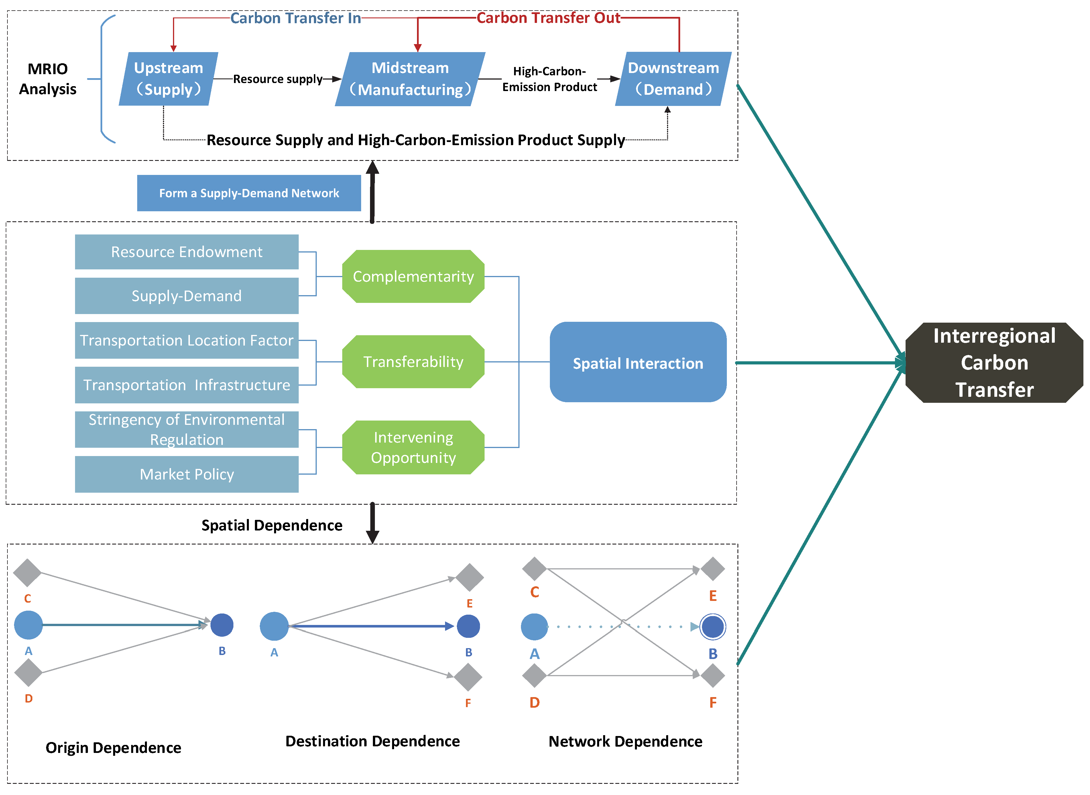
Spatial interactions constitute the fundamental transmission mechanism governing interregional carbon transfer, dynamically modulating its magnitude and directional pathways. Through complex crossregional supply–demand linkages, these interactions transform carbon transfers from linear chain transfers into a resilient, scale-free network topology. This architecture not only initiates emission redistribution but critically determines outcomes such as path-dependent flow trajectories through preferential attachment dynamics and spatially embedded dependencies via network spillover effects.
The role of spatial interactions in interregional carbon transfer can be categorized into three key functions: initiating carbon transfer, shaping the scale and pathways of carbon transfer, and modulating spatial dependencies. Spatial interactions act as the foundation for carbon transfer by connecting regions with differing resource endowments, demand patterns, and economic structures. Without spatial interaction, interregional exchanges of carbon-intensive products and resources cannot occur. By mediating the supply–demand network and influencing the transferability of resources and products, spatial interactions determine the magnitude and direction of carbon flows between regions. These pathways are influenced by factors such as infrastructure, policies, and economic conditions. Spatial interactions create complex dependencies between regions, linking carbon flows to the behaviors and characteristics of both origin and destination regions. This interdependence ensures that carbon transfer is influenced by the dynamics of multiple regional actors rather than isolated entities.
As formalized in
Figure 1, spatial interactions govern carbon transfer through supply–demand networks and geographic linkages. Complementarity represents the degree of matching between regional resources and demand, serving as the fundamental driver of spatial interactions. When one region faces a shortage of a specific product or resource while another region experiences a surplus, complementarity arises. This mismatch drives the flow of carbon embedded in goods and resources between regions. The degree of complementarity is primarily influenced by regional resource endowments and supply–demand relationships. For example, resource-rich regions in central and western China supply high-carbon products, such as raw materials and energy, to consumption-driven coastal areas, enabling carbon transfer through interregional trade. Transferability reflects the practical feasibility of supply–demand exchanges between regions, determined by the ability to overcome spatial barriers such as distance, time, and cost. Even with strong complementarity, if transportation costs are prohibitively high or geographic constraints exist, actual carbon transfer may not occur. This condition is heavily influenced by the quality of infrastructure and geographical proximity. For instance, regions connected by advanced rail or highway networks exhibit higher transferability, enabling smoother flows of high-carbon products and their associated emissions. Intervening opportunities refer to the role of external factors, such as economic changes or policy interventions, in disrupting or optimizing existing supply–demand relationships and carbon transfer pathways. For example, policy-driven incentives for clean energy or regulatory restrictions on high-carbon industries can alter the direction and magnitude of carbon transfer. Economic shifts, such as rising production costs or the introduction of new technologies, may prompt firms or regions to explore alternative suppliers or partners, reshaping carbon transfer dynamics.
Spatial interactions facilitate the formation of interregional supply–demand networks, which mediate carbon transfer along the supply chain and allocate carbon responsibility across regions. The supply chain underlying interregional carbon transfer can be divided into three key stages, the upstream stage, midstream stage, and downstream stage. The upstream stage involves resource extraction and preliminary processing, primarily producing raw materials with high amounts of embedded carbon emissions. The carbon transfer at this stage is typically low but is essential for supplying resources to downstream processes. Central and western regions, rich in energy and raw materials, are often the primary contributors at this stage. The midstream stage focuses on manufacturing and advanced processing. It represents the “core” of the supply chain, where carbon-intensive products are processed and embedded emissions peak. Industrially developed regions, such as those in central China, act as hubs for midstream activities, transferring processed goods to downstream regions. The downstream stage addresses the final consumption of products. These regions, often economically advanced with low-carbon industrial structures, serve as major recipients of high-carbon goods but contribute minimally to embedded emissions. Coastal regions such as the Yangtze River Delta typify downstream areas, driving demand for upstream extraction and midstream production through consumption. The interdependence of these supply chain stages creates a continuous feedback loop, with upstream regions providing resources for midstream production, midstream regions supplying carbon-intensive products to downstream areas, and downstream consumption stimulating demand for upstream extraction and midstream processing. This dynamic supply chain structure forms the backbone of interregional carbon transfer.
Due to spatial interactions, interregional carbon transfer does not follow a simple linear flow. Instead, it forms a dynamic network of multiple nodes and pathways, exhibiting significant spatial dependencies. These dependencies can be categorized into three types, origin dependence, destination dependence, and network dependence. Origin dependence indicates that carbon transfer is heavily influenced by the behavior of the originating region and its neighboring areas. For example, a developed region (Region A) and its surrounding areas (Regions C and D) may collectively transfer high-carbon products to an industrial hub (Region B). This behavior reflects the concentration of economic and industrial activities in origin regions and their immediate surroundings. Destination dependence refers to the reliance of carbon transfer on the receiving region and its surrounding areas. For instance, a downstream consumption hub (Region A) may source high-carbon products not only from an upstream industrial region (Region B) but also from its neighboring areas (Regions E and F). This highlights the clustering effect of high-carbon product flows around key consumption regions. Network dependence captures the complex interconnections between multiple nodes and pathways in carbon transfer. Carbon flows between origin regions (Region A and its neighboring Regions C and D) and destination regions (Region B and its neighboring Regions E and F) are mediated by intricate supply–demand networks, forming multi-node, multi-path closed loops. This dependency underscores the systemic nature of carbon transfer, driven by interactions within the broader spatial network.
Spatial interactions reshape interregional carbon transfer from a simple supply–demand exchange into a dynamic networked system, driven by economic, geographic, and policy factors. This mechanism highlights the need for targeted interventions to optimize carbon flows, including enhancing regional complementarity through strategic industrial layouts that balance resource endowments and consumption patterns, improving transferability by investing in infrastructure that reduces transportation costs and logistics inefficiencies, and leveraging intervening opportunities to guide carbon transfer toward low-carbon pathways using policy incentives and economic restructuring. By understanding the role of spatial interactions, policymakers can design more effective strategies to manage interregional carbon flows, mitigate carbon leakage risks, and foster collaborative carbon reduction across regions. This comprehensive perspective underscores the critical importance of spatial dynamics in achieving sustainable development and carbon neutrality goals.
4. Methodology
4.1. Regional Carbon Transfer Model Based on MRIO Table
From the perspective of spatial interactions, sectors in different regions are interconnected through intermediate inputs, forming a network of spatial dependencies of carbon transfer. Input–output analysis provides the foundation for quantifying supply and demand relationships between regions and sectors [
60]. Therefore, we employed the MRIO model to measure interprovincial carbon transfer and examine its determinants and spatial dependencies.
In the MRIO model, regions are represented with their unique technologies, and trade is classified into intermediate trade (trade between industries) and final trade (trade for final consumption). The basic input–output in region
r equation is
where
x denotes the vector of total output of each industry product of the region
r;
Arr is the intraregional production coefficient matrix;
Ars is the trade matrix, which captures the flow of intermediate goods between region
r and
s; and
yrr and
yrs are the final trade values, representing the demand for final products from region
s to region
r. Assuming there are now
m regions, each containing
n sectors, we extend the input–output equation of region
r to encompass the entire multiregional system. In matrix form, Equation (1) becomes
This can also be expressed in compact form by Equation (3):
Additionally, solving through the Leontief Inverse
and
I identity matrix of
and transferring the matrix form of Equation (3), we can obtain
Let
C be the block-diagonal environment intensity matrix:
Based on all the above equations, the all-regions carbon transfer matrix
E is as follows:
The expression for embodied carbon transfers from region
r to region
s triggered by regions
s’s consumption is given by
4.2. Spatial Correlation Index
Moran’s index (Moran’s I) is an important indicator for testing the existence of spatial autocorrelation and is widely used in spatial analysis. The equation of Moran’s I is as follows:
where
n represents the number of regions,
yi is the
i-th observation,
is the average variables of all regions, and
Wij is the spatial weight matrix. The value range of Global Moran’s I is [−1, 1]. A Moran’s I greater than zero indicates a positive spatial correlation, with higher values signifying stronger spatial autocorrelation or more pronounced clustering effects. A negative Moran’s I suggests a negative spatial correlation, meaning adjacent spatial units exhibit significant differences. A value of zero for Moran’s I implies a random spatial distribution, indicating no spatial correlation.
4.3. Study Design of Spatial Interaction of Carbon Transfer
The gravity model, derived from Newton’s law of universal gravitation, has been widely used in studying international trade, geographical economies, and regional networks [
61]. Traditional gravity models typically analyze individual flows without considering the spatial influences of the surrounding areas. This model, however, analyzes paired-flow data between two places in space, where each region can act as both an origin and a destination. The standard gravity model is shown in Equation (9):
where
denotes the flows between region
j and region
i, while
Xd(
i) and
Xo(
i) denote the destination and origin factor sizes and
G(
i,
j) represents the distance between them. In our study, we chose the road distance between provincial capitals as the spatial distance.
Based on the spatial relationships of interregional carbon transfers, illustrated in
Figure 1, the level of carbon transfer between two regions is influenced not only by their bilateral spatial interaction effects but also by the interconnected impacts among carbon-exporting regions and their neighbors, carbon-importing regions and their neighbors, and the neighboring regions of both the exporting and importing regions. This implies that interregional carbon transfer—our dependent variable—exhibits spatial interdependence.
To capture these complex spatial dynamics, we integrated the gravity model with a general spatial econometric framework following LeSage and Fischer [
62], Margaretic et al. [
63], and LeSage and Pace [
64]. This synthesis yielded a spatial autoregressive extended model (spatial OD model) for analyzing the spatial dependence and driving factors of interregional carbon transfers. The general specification is given by
In Equation (10), eod,t is the explanatory variable representing the carbon transfer from the origin to the destination, and is constructed by stacking the flow matrix . Similarly, g is the logged distance from G(i,j). Xo and Xd are the set of characteristic variables of the origin and destination. and , where X is an matrix of explanatory variables across n regions; Xd denotes the vector of destination-specific determinants of carbon transfers; and Xo represents the vector of origin-specific determinants. represents a Kronecker product, and is an vector of them.
Conventional geographical adjacency matrices fail to capture actual transport costs, while distance matrices derived from latitude–longitude coordinates overlook terrain and transportation networks. Furthermore, spatial weight matrices based solely on economic disparities neglect physical accessibility. To address these limitations, we construct a spatial weight matrix W by integrating railway travel time and economic disparity across regions.
Where , and . Wdy is the carbon transfer destination-based dependence spatial lag, representing spatially weighted average carbon transfers in destination-linked regions. Woy is the carbon transfer origin-based dependence spatial lag, representing spatially weighted average carbon transfers in origin-linked regions. Wwy is the carbon transfer network dependence spatial lag, representing spatially weighted average carbon transfers in regions linked to both origins and destinations. The coefficients , , and quantify the intensity of destination-based, origin-based, and network spatial dependence, respectively.
4.4. Scalar Summary Estimates for Spatial Model
The coefficients in the spatial interaction model do not directly represent the impact of changes in factors between regions on interprovincial carbon transfer. To address this, a partial differential estimation method is used, which breaks down the effects into origin, destination, and network effects in order to analyze the determinants of interprovincial carbon transfer.
The partial derivatives reflecting the total effects for this model are as follows:
where
is an
matrix of zeros with the
i-th row equal to
, and
is an
matrix of zeros with the
i-th column equal to
.
A scalar measure of the
origin effect can be based on
, where
OE is the
matrix defined in Equation (12).
is the matrix adjusted to have a zero in the i, i-th row and column element. This adjustment separates the intraregional effect.
Similarly, we can produce a scalar summary measure of
destination effects using
, where
DE is the
matrix defined in Equation (13).
The matrix is adjusted to have a zero in the i, i-th row and column element. This adjustment separates the intraregional effect.
Scalar summary measures of the (average) origin and destination effects can proceed in an obvious way, while the scalar summary for (cumulated)
network effect (
ne) can be calculated as
,
, where
NE is an
matrix analogous to those previously defined.
, where is an matrix of ones.
4.5. Variables
To capture the dynamics of spatial interactions, we select ten explanatory variables spanning three dimensions of spatial interaction mechanisms—complementarity, transferability, and intervening opportunities—based on the carbon transfer pathways illustrated in
Figure 1. Additionally, to ensure comprehensive coverage of driving factors, we incorporate three control variables: technological innovation capacity, green governance capability, and consumption potential (
Table 1).
Complementarity: This dimension captures the fundamental drivers of carbon transfers arising from disparities in regional resource endowments and demand patterns. For Economic Gradient (Eco_C), per capita GDP differentials reflect industrial specialization demands. Higher-income provinces relocate carbon-intensive industries to lower-income regions via trade, quantifying the pull effect of economic disparities on carbon transfers. Interprovincial Coal Redistribution (Res_C): As direct carriers of embodied carbon, interregional energy flows quantify energy complementarity. Railway coal transfers directly capture supply-chain-driven carbon redistribution. Industrial Land Allocation (Ind_L) measures the dynamic matching of comparative advantages in manufacturing. This spatial–industrial matching constitutes the structural driver of carbon relocation. Carbon Efficiency Gap (En_C) reflects technology-induced carbon transfers, where regions with lower carbon productivity become net importers of embodied emissions.
Transferability: Network Brokerage Centrality (Trans_I) measures a province’s role as a supply chain intermediary using betweenness centrality. High-centrality nodes act as structural brokers in carbon transfer networks, bridging upstream suppliers and downstream consumers. Infrastructure Nodal Density (Trans_D) captures the spatial coverage of transport infrastructure. Regions with higher nodal density exhibit lower spatial friction, facilitating factor mobility and reducing resistance to embodied carbon flows. Transport Infrastructure Land (Trans_L) measures long-term freight capacity through dedicated transportation land allocation. This variable directly influences bulk commodity flow efficiency—a critical conduit for embodied carbon transfers.
Intervening opportunities: Fixed-Asset Investment Intensity (Cap_I) measures path dependency in investment-driven carbon relocation. Regions with excessive capital formation attract carbon-intensive industries, inducing carbon lock-in effects via sunk investments in high-emission infrastructure. Pollution Abatement Investment (Env_G) quantifies the crowding-out effect of environmental regulation, including enhanced local abatement incentives. Marketization Index (Gov_I) reflects the efficiency of market-based resource allocation. Higher marketization enables emission displacement through market mechanisms (e.g., carbon credit trading, green supply chain contracts).
Control variables: Regional Wage Premium (Res_PP) reflects interregional labor cost differentials that drive industrial relocation—the core mechanism of the pollution haven hypothesis. Higher wages increase compliance costs, inducing the outmigration of carbon-intensive sectors. Green Innovation Intensity (Tech_D), measured by utility model patent grants, captures localized innovation capacity. Technological spillovers reduce carbon intensity in connected regions, controlling for innovation-driven pathway interference. Carbon Sink Land (Env_S) quantifies ecological carbon sequestration services through designated green spaces. This variable controls for local carbon absorption capacity that may offset transferred emissions.
4.6. Data Collection and Processing
The 2012, 2015, and 2017 MRIO tables of China’s 30 and 42 sectors (
Table 2) used in this paper were from the Carbon Emission Accounts and Datasets (CEADs) [
65,
66]. The data on various energy activity levels came from the “
China Energy Statistical Yearbook” of the corresponding year. Emission factors mainly came from the “
2006 IPCC National Greenhouse Gas Inventory Guidelines” and “
Provincial Greenhouse Gas Inventory Guidelines (Trial)”. Due to the poor availability of data for Tibet, this study excluded data for Tibet from the MRIO table.
We selected the years 2012, 2015, and 2017 as the research time periods for the following reasons: (1) Temporal Representativeness: The year 2012 marks the transition of China’s economy from high-speed growth to medium-to-high-speed growth. The year 2015 is significant as it was China signed the Paris Agreement, signaling a commitment to intensified climate action. By 2017, the effects of these policies had gradually become evident. (2) Data Availability Comparability: The latest publicly available data from the CEADs dates only to 2017. Considering data availability and timeliness, the selection of 2012, 2015 and 2017 ensured access to comprehensive and reliable MRIO tables, facilitating meaningful comparisons across different periods.
Given that interprovincial input–output relationships tend to remain relatively stable in the short term, the findings of this study are expected to provide valuable insights for future research and policy development within a reasonable timeframe. Owing to the massive datasets utilized in this research, every parameter estimate reported in this paper was computed using MATLAB 2024b.
5. Results and Analysis
5.1. Measurement of Carbon Transfer
Based on the MRIO model and related data, carbon transfers in China’s interprovincial regions were measured and accounted for using MTLAB 2024b, as shown in
Figure 2.
Interprovincial carbon emissions driven by trade activities in China have shown a consistent upward trend, although the rate of increase has gradually declined in recent years. In 2012, trade-related carbon emissions amounted to 4406.775 Mt, rising to 4825.485 Mt in 2015 and further to 4954.605 Mt in 2017. The trend of change is consistent with the findings of existing studies [
67]. From a spatial perspective, carbon transfer primarily occurs between central China and the eastern coastal regions, while transfers involving the western regions are relatively minimal. In 2012, most interprovincial carbon transfer occurred within the eastern region of China. By 2017, carbon transfers between the eastern and central regions had significantly increased, revealing a spatial trend characterized by “westward” and “northward” movements of carbon flows.
Provinces in the eastern and southern coastal areas serve as major sources of carbon emissions. For instance, Guangdong Province primarily exports carbon emissions to Hebei, Inner Mongolia, Shandong, Henan, and Jiangsu Provinces. Zhejiang Province transfers emissions mainly to Hebei, Inner Mongolia, Henan, Shandong, and Liaoning Provinces. Provinces in the central region, such as Hebei and Inner Mongolia, are the primary recipients of carbon transfers. Hebei Province receives carbon emissions predominantly from Guangdong, Jiangsu, Zhejiang, Henan, and Beijing. Inner Mongolia imports emissions primarily from Guangdong, Jiangsu, Beijing, Zhejiang, and Henan.
The results indicate that interprovincial carbon transfer networks exhibit significant spatial dependencies, which can be categorized into three types: destination dependence, origin dependence, and network dependence. Carbon transfer networks demonstrate strong reliance on destination regions. For example, provinces such as Inner Mongolia and Hebei act as key destinations for carbon emissions, and their neighboring provinces also tend to receive significant carbon transfers. This indicates that destination provinces play a central role in shaping the spatial structure of carbon transfer networks. Provinces such as Jiangsu, Shanghai, and Zhejiang are major origins of carbon transfers. These provinces are geographically adjacent, forming a concentrated cluster of high-carbon outflows. This highlights the spatial dependency on origin regions, where neighboring provinces collectively contribute to carbon transfers. Carbon transfers in China are influenced by complex interactions across multiple nodes in the network. For instance, if Zhejiang Province serves as a primary origin and Hebei Province as a primary destination, neighboring origin provinces (e.g., Jiangsu and Shanghai) predominantly transfer carbon emissions to regions adjacent to Hebei (e.g., Inner Mongolia, Shanxi, and Shandong). This demonstrates the network dependency in interprovincial carbon transfers, where spatial interactions are mediated through multi-node, multi-pathway networks.
5.2. Spatial Interaction Analysis of Carbon Transfer
5.2.1. Spatial Autocorrelation Test
Interregional carbon transfer is likely influenced by neighboring regions, making it essential to test for spatial correlation before analyzing the factors affecting carbon transfer. To determine whether interregional carbon transfer exhibits spatial dependence, a spatial autocorrelation model was employed. If significant spatial correlation was identified, spatial econometric models were required for further analysis of the influencing factors.
Table 3 presents the Global Moran Index (Moran’s I) for interregional carbon transfer under three different spatial weight matrices. Given the potential spatial dependencies among the
origin,
destination, and
network during the carbon emission transfer process, three distinct spatial weight matrices—
Wd,
Wo, and
Ww—were constructed in the preceding section. Accordingly, it was necessary to test the spatial autocorrelation of carbon transfer under each of these spatial configurations to ensure the robustness of the subsequent spatial econometric analysis. The results demonstrate that Moran’s I values are all greater than 0 and statistically significant at the 0.01 level across all three weight matrices. This indicates that interregional carbon transfer exhibits significant spatial clustering and a positive spatial correlation.
Table 4 reports Global Moran’s I statistics for all explanatory variables during 2012–2017. The results demonstrate statistically significant spatial clustering patterns. Ind_L exhibits negative spatial dependence (Moran’s I < 0), indicating a dispersed distribution of manufacturing zones. All other variables show positive spatial dependence (Moran’s I > 0), confirming regional spillover effects.
5.2.2. The Analysis of Interaction and Determinants
Provincial carbon transfer matrices were constructed using a multiregional input–output (MRIO) framework. Spatial econometric specifications in
Table 5 were estimated with travel-time-based weights (Equation (10)), accounting for interregional connectivity dynamics. To address methodological challenges of directional flow data and ensure robust inference, we implement a Bayesian Model Averaging (BMA) framework integrated with Markov Chain Monte Carlo Model Composition (MC
3). This approach explicitly models spatial dependence in carbon flow networks while mitigating model uncertainty.
To accurately distinguish the roles of the origin and destination regions in the spatial OD model, the same explanatory variables are used for both roles, with the prefixes “O_” and “D_” added to the variable names. This notation clearly differentiates the effects of the variables when a region acts as the origin or the destination of carbon transfers. This approach ensures consistency in variable selection while capturing the asymmetric effects of economic, environmental, and regional factors on interprovincial carbon transfers. The distinction between “O_” and “D_” also facilitates precise estimation of the push and pull factors driving carbon transfers across provinces.
Table 5 shows that interregional carbon transfer demonstrates significant positive spatial dependence. Three types of spatial dependence—
origin dependence (
),
destination dependence (
), and
network dependence (
)—were found to exist simultaneously. The coefficient for
origin dependence shows a declining trend over time. While carbon transfers from origin regions to the same destination are still influenced by neighboring regions, the dominance of origin regions is decreasing. This reflects a shift towards a more distributed pattern of carbon transfer. The
destination dependence coefficient exhibits a statistically significant inverted U-shaped pattern, The positive coefficient estimates confirm that carbon transfers between origin and destination, cascading spillovers to hinterland regions surrounding the origin and amplified transfer intensity in the destination’s adjacent areas.
Network dependence follows a “U-shaped” trend, suggesting that the connections between origin and destination regions remain strong and exhibit clear network characteristics. For example, coal from resource-rich regions like Shanxi and Inner Mongolia often passes through intermediary regions (e.g., Henan) before reaching industrial hubs in eastern coastal areas such as Jiangsu and Guangdong. Policies like the Belt and Road Initiative have further strengthened economic and resource linkages between regions, enhancing network dependence in carbon transfer.
Comparative analysis reveals a fundamental transition in China’s interprovincial carbon transfer drivers: from initial origin supply-push dominance to destination demand-pull dynamics, culminating in networked flows. The persistent strength of origin dependence reflects the competitive strategies of early-developing regions local governments compete in ecological modernization to upgrade economic quality, while firms engage in herding behavior toward common destinations for market capture and risk mitigation. The 2015 inflection point—coinciding with China’s 13th Five-Year Plan launch—witnessed coastal provinces (e.g., Guangdong, Zhejiang) accelerating carbon-intensive imports to fuel investment expansion. Meanwhile, late-developing regions enhanced carbon transfer receptivity through transport infrastructure upgrades, preferential investment policies and improved population attraction capacity.
In 2012, 2015, and 2017, the distance (g) was consistently negative, indicating a distance negative effect in interregional carbon transfer. Spatial distance historically amplified carbon transfer barriers through market fragmentation, where increasing geographical separation, such as elevated transport cost, constrained crossregional industrial linkages, and reinforced local protectionism. Infrastructure modernization has progressively attenuated this distance decay, where transport upgrades reduce effective economic distance, enabling frictionless supply chain integration and reconfiguration of pollution havens beyond traditional cores. For other explanatory variables, our analysis will identify and quantify the distinct effects of contributing factors on carbon transfer through origin effects, destination effects, and network effects in the following section.
5.3. Effects Estimates of the Interaction of Carbon Transfer
Spatial dependence implies that changes in one variable can lead to variations in carbon transfer volumes in both local and neighboring regions. These changes are further propagated through spatial feedback effects, influencing the original region in return. Based on Equation (11) to Equation (14),
Table 6,
Table 7 and
Table 8 report the
origin effects,
destination effects,
network effects, and their statistical significance for each explanatory variable. It can be observed that, with the continuous development of transportation infrastructure and across different spatial weight matrices, all variables except regional economic development level (Eco_C), transportation land use (Trans_L), and government market intervention (Gov_I) exhibit statistically significant and directionally consistent impacts on interregional carbon transfer across various years. This indicates robust findings for the origin effects, destination effects, and network effects of these explanatory variables.
5.3.1. Origin Effects
The origin effect reflects the direct impact of local characteristic changes on carbon relocation from the region, indicating the “push force” of carbon transfer generated by certain regions’ inherent attributes. From the perspective of complementarity indicators, each indicator demonstrates stable and significant effects on interregional carbon transfer across different development stages. Regional economic development level and industrial land use (Ind_L) exhibit significantly negative impacts on interregional carbon transfer, while interregional coal exchange volume (Res_C) and energy intensity (En_C) show significantly positive effects. In economically developed regions, industrial restructuring—characterized by an increased share of service sector value added and decreased share of secondary industries like manufacturing—stimulates the decline of high-carbon industries. This drives local industries toward green and low-carbon transition, enhances energy efficiency, and reduces energy intensity. Consequently, the scale of local carbon relocation is inversely related to economic development level but positively correlated with energy intensity. Increased interregional coal exchange volume expands local coal-related industries and boosts high-carbon production capacity. Simultaneously, the expansion of industrial land mitigates the industrial “crowding-out effect” caused by economic development in carbon relocation origins, reduces corporate relocation costs, and diminishes the “crowding-out effect” on high-carbon industries locally. These dynamics thereby reduce the scale of carbon relocation between regions.
The transport transferability indicator captures a region’s capacity to facilitate industrial relocation. Enhanced hub centrality (Trans_I) and upgraded transportation infrastructure (Trans_L) improve local resource allocation efficiency while reducing interregional corporate relocation costs. This promotes the transfer of high-carbon industries to peripheral regions, thereby increasing interregional carbon transfer. Conversely, higher integrated node density (Trans_D) generates countervailing effects: (1) by reducing regulatory facilities’ service radii, it heightens exposure risks for high-carbon transfers and discourages crossregional investments, thereby suppressing interregional carbon transfer, while (2) dispersing transportation hubs within the region localizes transport-facilitated carbon transfers and reduces extraregional transfer volumes.
Intervention opportunity indicators serve as proxies for the intensity of local government protectionism. An increase in fixed-asset investment (Cap_I) accelerates local industrial upgrading, thereby diminishing the demand for relocating high-carbon production capacity. Rising pollution control investment (Env_G) signifies improvements in regional energy cleanliness. Initially, heightened environmental governance costs incentivize both governments and enterprises to relocate high-carbon industries, resulting in a positive association between pollution control investment and interregional carbon transfer during the early study period. Subsequently, as technological advancements yield emission reduction effects, local production progressively transitions toward cleaner, low-carbon models. Concurrently, economic development drives the relocation of certain high-carbon enterprises, further reducing the demand for carbon transfer. Consequently, pollution control investment demonstrates a significantly negative correlation with interregional carbon transfer in later stages. The level of marketization (Gov_I) is positively correlated with enhanced regional resource allocation efficiency. As of 2012, China’s average marketization index stood at merely 5.8 (Fan Gang Index, on a 0–10 scale), indicating that interprovincial factor mobility remained significantly hindered by local protectionism and administrative barriers. This suppressed marketization’s regulatory effect on carbon transfer. However, through concerted nationwide efforts to establish a unified market and continuous improvements in marketization, interregional synergistic effects have deepened via positive feedback loops. This evolution enables local green transitions to substitute for industrial relocation, ultimately reducing interregional carbon transfer volumes.
5.3.2. Destination Effects
The destination effect captures how shifts in exogenous regional characteristics generate attraction for carbon inflows, constituting the “pull force” of interregional carbon transfer. Regional investment capacity exerts a consistently significant negative effect on inflow attractiveness. Marketization levels suppress carbon inflows only upon reaching advanced developmental stages. Interregional energy exchange volume and local energy intensity exert significant positive effects on inflow attractiveness. Local economic development demonstrates statistically insignificant effects overall, with only marginally negative coefficients during the study period’s initial phase. Industrial land area exhibits moderate yet significant negative effects on carbon attraction relative to other determinants.
Transferability demonstrates limited influence on carbon transfer, while transportation infrastructure land area exhibits unstable effects. Network betweenness centrality and regional node density exert stable yet opposing impacts on interregional carbon transfers. Increased network centrality reduces physical transaction costs between regions, stimulating factor mobility and thereby promoting carbon inflows. Elevated regional node density enhances local accessibility and land value, primarily attracting high-value-added, low-energy, low-emission enterprises (e.g., advanced services, high-tech industries), consequently diminishing demand for high-carbon industries.
Distinct from other variables, local pollution control investment (Env_G) exerts a significant yet unstable impact on interregional carbon inflow attraction. During the early research period, regions with higher environmental investment—such as Shaanxi and Inner Mongolia—maintained comparatively lax environmental regulations while possessing abundant resource endowments that supported emission-intensive industries. The majority of pollution control investments during this phase funded end-of-pipe treatment facilities, which failed to meaningfully reduce regional attractiveness to high-emission industries, thereby materializing the “pollution haven” effect. However, the implementation of China’s amended Environmental Protection Law in January 2015 significantly increased penalties for corporate pollution violations, fundamentally transforming the nature of environmental investments from end-of-pipe solutions toward source reduction and industrial structural adjustment. This regulatory shift accelerated the phase-out of backward production capacity, led enterprises to adopt cleaner low-carbon technologies through process innovation, and ultimately elevated green entry barriers for businesses, consequently diminishing regional carbon inflow attraction.
5.3.3. Network Effects
Network effects capture the amplification and spillover mechanisms through which interregional connectivity structures propagate and intensify carbon transfer, signifying the transmission and reinforcement functions of spatial association networks in crossregional carbon redistribution. Such effects dominate regional carbon transfer dynamics primarily due to multiplier amplification within spatial interactions and systemic self-reinforcement mechanisms. Prevailing spatial analyses of interregional carbon transfer have predominantly focused on conventional bilateral origin–destination frameworks while overlooking third-party feedback loops. For instance, when Jiangsu Province elevates local coal flows or enhances transportation infrastructure, origin effects increase its carbon outflow volume, with most emissions transferring to the geographically proximate Anhui Province. Upon receiving these transfers, Anhui’s expanded energy demand subsequently triggers increased coal flows through power grids to Shanxi Province, ultimately elevating Shanxi’s carbon transfer volume.
Among network effects, the indicator exhibiting the most pronounced change in its impact on interregional carbon transfer is transportation infrastructure footprint. In 2012, the influence of transportation infrastructure land area on carbon transfer remained relatively modest, with statistically insignificant effects observed in 2015. However, by 2017, it demonstrated a significantly positive impact. Between 2012 and 2017, China’s transportation infrastructure land expanded from 5724.68 km2 to 8341.41 km2. This rapid capacity expansion enhanced interregional connectivity, directly intensifying economic linkages and network effects across regions. Concurrently, transportation infrastructure development stimulated land development along corridors, amplifying local fixed-asset investment and economic growth, thereby increasing the absolute scale of carbon transfer. Furthermore, such investments elevate regional importance as transportation hubs, creating dense networks that “lock in” existing spatial economic patterns and logistics pathways. This path dependency generates nonlinear growth trajectories in carbon transfer impacts over time. Ultimately, massive and efficient transportation infrastructure constructs broader, more permeable “highways” for carbon transfer, substantially facilitating the movement of emissions from production sources to final consumption sites.
6. Conclusions and Policy Recommendations
6.1. Conclusions
This study investigates interprovincial carbon transfer in China, using a MRIO model and spatial interaction models to systematically analyze the influencing factors and dynamic characteristics of carbon transfer across regions in 2012, 2015, and 2017. The findings offer key insights into the spatial dependencies and interactive dynamics of carbon transfers.
During 2012–2017, China’s interregional carbon transfer volume increased from 9080.8 Mt to 9391.5 Mt. This transfer exhibited pronounced spatial concentration in central and eastern regions, with the eastern region serving as the primary carbon-export hub and the central region functioning as the dominant carbon-import zone. Western provinces demonstrated minimal interprovincial carbon transfer, while transfers between central/eastern and western regions remained constrained by spatial distance factors. As aggregate transfer volumes rose, peak regional values progressively declined and high-transfer clusters became less concentrated, indicating a gradual equalization of carbon redistribution patterns across regions.
Interregional carbon transfer is influenced by multiple factors that collectively shape spatial–industrial linkages and consequently affect carbon redistribution patterns. Spatial econometric modeling reveals that as relative spatial distances between regions diminish, carbon transfer exhibits stable and significantly positive dependencies on origin regions, destination regions, and network structures. Origin dependence weakens with shrinking spatial distances and destination dependence follows an inverted U-shaped trajectory, while network dependence demonstrates a V-shaped evolutionary pattern. In 2012, origin dependence dominated interregional carbon transfers, and the dominant type shifted to destination dependence by 2015 and transitioned to network dependence in 2017. This staged transition in spatial dependencies reflects the evolution of China’s carbon transfer mechanisms—from locally driven to locationally attracted, and ultimately to network-dominated redistribution. Such progression necessitates upgrading carbon governance strategies toward a “network-channel governance” paradigm.
The spatial decomposition of contributing variables reveals that interregional carbon transfer constitutes an inherently networked phenomenon rather than a bilateral process. The estimation of origin, destination, and network effects demonstrates significant spatial influences across most interactive factors, with network effects exhibiting predominant importance. Among complementary effects, regional economic development and industrial land expansion exert modest inhibitory impacts on carbon transfer, whereas reducing interregional coal flows and regional energy intensity proves substantially effective. The spatial effects of transferability variables indicate that transportation networks manifest dual-directional impacts: moderating infrastructure land occupation, reducing transport hub functionality, and enhancing integrated node density collectively mitigate carbon transfers. The analysis of regional opportunity variables shows that increased pollution control investments initially impede but subsequently suppress carbon transfer as funding escalates. Similarly, free-market development exerts negligible initial influence but ultimately exerts the strongest inhibitory effect as market mechanisms mature.
6.2. Policy Recommendations
This study offers significant policy implications for informing low-carbon pathways and carbon mitigation strategies in China and beyond.
First, land functions not merely as a factor endowment but as a critical spatial lever for climate governance. The strategic allocation of industrial and transportation infrastructure land reconfigures regional economic geography through dual mechanisms: Transportation land expansion reduces logistics costs, thereby enabling pollution-intensive industries to relocate toward regions with lenient environmental regulations, while simultaneously extending economic radiation ranges that intensify long-distance trade and elevate transportation-related carbon transfers. Conversely, moderate industrial land expansion—particularly through clustered industrial parks—facilitates low-carbon technology diffusion, whereas localized industrial chains reduce embodied carbon emissions from crossregional intermediate goods transport. Effective implementation requires industrial land optimization to promote multi-story factories achieving vertical agglomeration (reducing per-unit output energy intensity) and deploy centralized monitoring networks that internalize regulatory externalities across industrial clusters. Concurrently, transportation land governance must increase integrated node density proportionally with infrastructure expansion, co-locate emissions monitoring stations at critical junctions, and implement mandatory carbon leakage assessments during highway planning to evaluate high-carbon industry relocation risks—collectively transforming land use systems into precision instruments for low-carbon spatial restructuring.
The second imperative involves coordinated governance and market mechanisms, strengthening the market’s decisive role in resource allocation for regional low-carbon development. Empowering markets to effectively leverage their inherent resource allocation functions is crucial for advancing low-carbon economic transformation. On one front, deepening energy price marketization reforms is essential—transitioning government functions from price-setting to market supervision, progressively liberalizing competitive energy sectors, and fostering diversified energy trading centers. This enables price signals to guide supply–demand dynamics, harnessing market-based incentives to drive voluntary emission reductions among producers and consumers. On another front, enhancing the development and operation of regional carbon trading markets is paramount. This requires establishing robust carbon emission disclosure mechanisms, extending sectoral coverage based on linear expansion methodologies, and progressively scaling market breadth and depth.
Third, establishing regional low-carbon coordination mechanisms is imperative. Given the statistically significant origin, destination, and network effects in crossregional carbon transfers, climate policies adopted by individual jurisdictions inevitably generate spillover impacts through geographic and economic linkages. Consequently, subnational governments must recognize the criticality of coordinated development for achieving cost-effective decarbonization. This necessitates the collaborative exploration of mutual trust-building frameworks, the creation of energy conservation and emission reduction data-sharing networks, and the joint implementation of emission control schemes. Such institutionalized cooperation enables individual regions to pursue cost-minimizing pathways toward emission reduction within collective carbon constraints.
In summary, this study advances the understanding of spatial dependence in interregional carbon transfer through spatial interaction analysis. Our spatial econometric regressions establish carbon transfer networks as the dominant influencing factor while introducing novel spatial perspectives on global transfer dynamics. We further develop evidence-based policy recommendations grounded in the tripartite framework of carbon transfer complementarity, transferability, and intervention opportunities.
Limitations and future research: (1) Temporal constraints arising from China’s interregional input–output table update cycle limit our analysis to 2012, 2015, and 2017 data. While the interregional input–output relationships remained relatively stable during this period, significant shifts in other determinants necessitate extended temporal coverage for more robust inference. (2) Given the complex flow-data network structure of interregional carbon transfers, future research should employ finer-grained geographical targeting to enhance spatial effect analysis of determinants.


