Impacts of Landscape Composition on Land Surface Temperature in Expanding Desert Cities: A Case Study in Arizona, USA

Abstract

Surface urban heat island (SUHI) effects are intensifying in arid desert cities due to rapid urban expansion, limited vegetation, and increasing impervious and barren land surfaces. This leads to serious ecological and socio-environmental challenges in cities. This study investigates the relationship between landscape composition and land surface temperature (LST) in Phoenix and Tucson, two rapidly growing cities located in the Sonoran Desert of the southwestern United States. Landsat-9 OLI-2/TIRS-2 satellite imagery was used to derive the LST value and calculate spectral indices. A multi-resolution grid-based approach was applied to assess spatial correlations between land cover and mean LST across varying spatial scales. The strongest positive correlations were observed with barren land, followed by impervious surfaces, while green space showed a negative correlation. Furthermore, the Urban Thermal Field Variation Index (UTFVI) and the Ecological Evaluation Index (EEI) assessments indicated that over one-third of both cities are exposed to strong SUHI effects and poor ecological quality. The findings highlight the critical need for ecologically sensitive urban planning, emphasizing the importance of the morphological structure of cities, the necessity of planning holistic blue–green infrastructure systems, and the importance of reducing impervious surfaces to decrease LST, mitigate SUHI and SUHI impacts, and increase urban resilience in desert environments. These results provide evidence-based guidance for landscape planning and climate adaptation in hyper-arid urban environments.

1. Introduction

Global climate change has led to significant alterations in the world’s climatic characteristics over the past century. The primary driver of these changes is anthropogenic activity [1,2]. In particular, the rapid increase in the global population has accelerated the expansion and intensification of urbanization [3,4]. The impervious surfaces and artificial structures that emerge during urbanization have caused the fragmentation, reduction, or complete disappearance of natural areas in certain regions. As a result, ecosystems have been damaged and ecological balance has been increasingly disrupted over time [5,6].

Cities have a complex structure due to the influence of numerous different natural and cultural factors. For this reason, the limiting factors such as the use of a single criterion or index [7], the evaluation of a certain small region, and the insufficient number and frequency of measurements negatively affect the accuracy and efficiency of the study results [8]. However, the development of Geographic Information Systems (GISs) and remote sensing technologies has significantly contributed to studies on landscape composition, climatic characteristics, and ecosystem structures of cities [5,9,10]. These technologies have especially facilitated the spatio-temporal monitoring and analysis of dynamic urban phenomena [11,12]. Landsat satellite imagery, which launched in 1972, has a long uninterrupted time series until today and covers large areas; thus, it can provide more detailed data in a short time compared to data obtained from traditional field measurements [13]. In this way, changes in land use/land cover (LULC) from the past to the present can be rapidly analyzed.

The rapid increase in urbanization plays a significant role in the emergence of various climatic and environmental problems that threaten human health and well-being [3,14,15]. One of the most notable phenomena among these problems is UHI [16,17,18,19]. The extreme UHI effect in cities leads to serious issues such as energy consumption, air pollution, water scarcity, heat waves, etc. and poses significant social, environmental, and economic impacts for the individuals in the cities, notably in terms of health [20,21,22,23].

UHIs are categorized into three groups according to the layer where heat is generated and measurement methods. These are surface urban heat island (SUHI), canopy urban heat island (CUHI), and boundary-layer urban heat island (BLUHI) [24,25,26,27]. SUHI refers to the heating level of urban surfaces based on land surface temperature (LST) data from satellite imagery and is widely used to compare urban–rural surface temperatures [28,29,30]. CUHI focuses on the difference in air temperature in the layer of the atmosphere nearest to the layer of human habitation and is usually measured by meteorological stations [31]. BLUHI, which is less common but is used in atmospheric modeling, describes the heat effect of urban areas on higher atmospheric layers [26,32]. This classification reveals the multi-layered phenomenon of UHIs and shows that each type requires different methods of analysis and different planning strategies.

SUHIs are caused by the proliferation of artificial surfaces (e.g., concrete and asphalt) in urban areas, the presence of heat-absorbing materials in buildings, the decrease in green space and vegetation cover, and alterations in landscape compositions [33,34,35]. Studies presenting projections for the future have revealed that the population in cities will increase and urbanization will continue at a rapid pace [36,37]. This suggests that unless effective mitigation measures are implemented, the adverse impacts of SUHIs will continue to intensify. Therefore, studies on SUHIs are essential for understanding urban temperature dynamics, identifying heat-vulnerable areas, and developing targeted mitigation strategies [6,38].

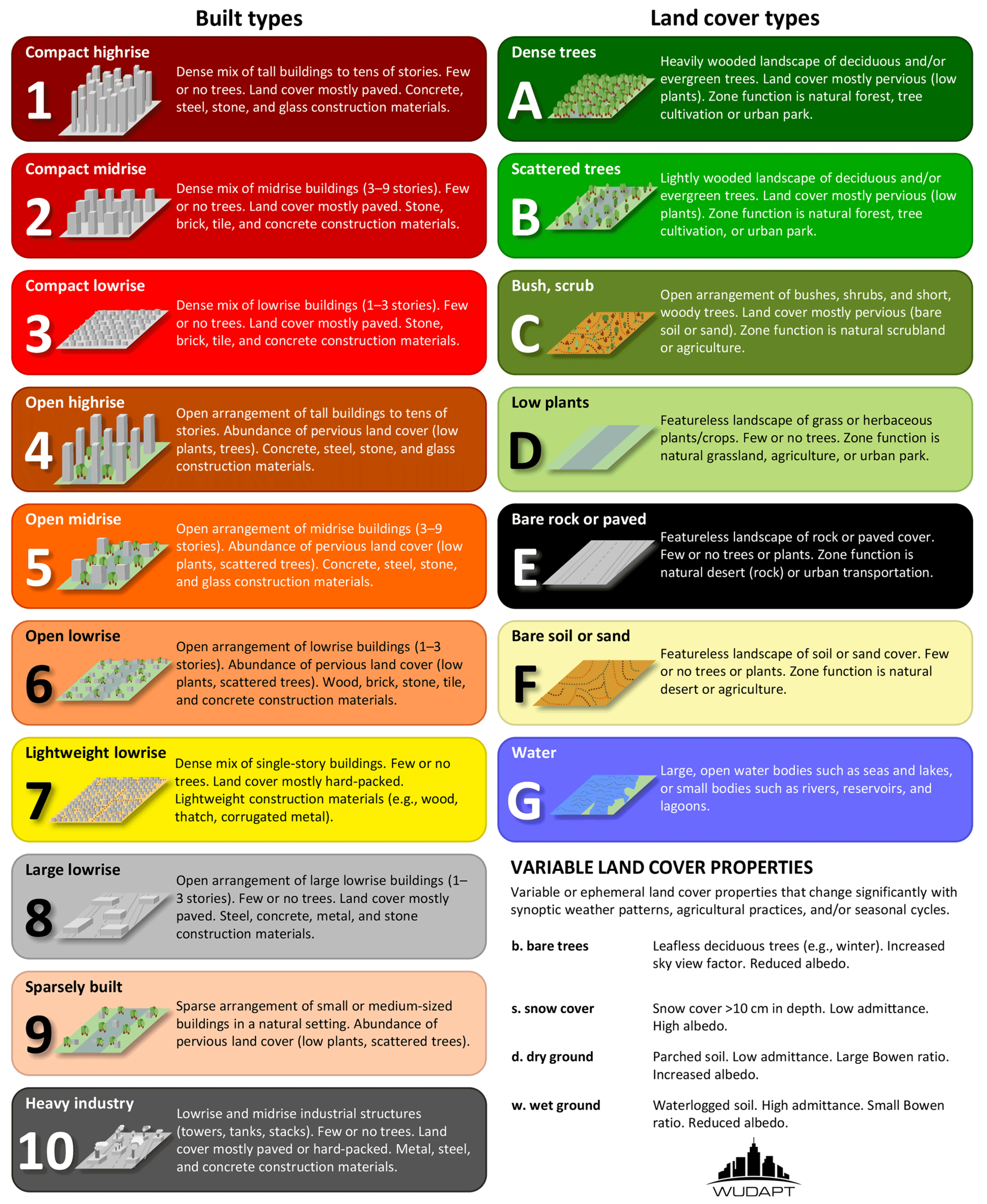
The local climate zone (LCZ) classification system was developed by Stewart and Oke [39] to assess thermal differences in urban areas in more detail and to calculate LST and SUHI events in standardized classified areas. The LCZ classification system categorizes cities into 17 different types based on physical characteristics such as building density, building height, and land cover. The first 10 types include built types (e.g., compact mid-rise, open low-rise, and sparsely built) and 7 types include land types (e.g., scattered trees, low plants, bare soil, or sand) [39,40,41]. In this context, LCZs provide a standardized framework for urban and rural SUHI assessments [42,43,44]. Thus, the effects of different forms of building and land uses on LST could be revealed in more detail [39,45].

The LULC is one of the most influential factors affecting the SUHI calculated from LST data. LULC types in regions with varying climatic conditions exhibit different levels of reflectivity and therefore require classification using appropriate spectral indices. To identify and analyze LULC, through Landsat satellite images capable of producing spectral indices, different indices such as the Normalized Difference Vegetation Index (NDVI), the Modified Normalized Difference Water Index (MNDWI), the Visible Red-Based Built-Up Indices (VrNIR-BI), and Dry Bare-Soil Index (DBSI) are used [46]. The NDVI is used to determine the density and assess the health of vegetation in the studied region, while the MNDWI is effective in identifying water surfaces in urban areas [47]. The VrNIR-BI helps distinguish impervious surfaces from vegetation and pervious surfaces [36], and the DBSI is employed to detect bare-soil coverage [48]. In addition to these, different spectral indexes such as LST and the Urban Thermal Field Variation Index (UTFVI) are widely used to obtain rapid and accurate results in large-scale SUHI studies [46]. These spectral indices are essential for evaluating the ecosystem services and ecological structures of urban areas. LST, which provides direct information about surface temperature, is an important parameter in revealing local and regional climate dynamics. Since LST provides climate information that helps to understand and analyze urban climate, the relationship between LST, and urban sprawl and landscape compositions has been widely examined in the literature [49,50]. Evaluating SUHIs and the UTFVI in conjunction with the NDVI and LST indexes enables more comprehensive assessments of both the climatic and ecological structure of the region [51,52,53,54].

Landscape compositional–structural interactions drive the dynamics and intensity of LST and SUHI variability [28,55]. For example, impervious surfaces and barren land can increase LST due to high heat absorption and low evaporative–transpiration capacity, while green spaces and water surfaces can improve thermal comfort through shading and evaporative cooling [55,56]. However, these effects depend not only on the presence of land cover types but also on the landscape’s structural characteristics (fragmentation, diversity, and connectivity) [56,57]. The strong relationship between the urban composition and spatial configuration of Phoenix and Tucson, and the urban heat island impact is estimated to cause these cities to heat up about six times faster than other cities [58]. In this context, landscape metrics are used to quantitatively evaluate these structural characteristics of the landscape. Metrics such as Shannon’s Diversity Index (SHDI) and the Landscape Shape Index (LSI) measure the heterogeneity and shape complexity of the landscape, while the Contagion Index (CONTAG) and the Landscape Division Index (DIVISION) reveal the degree of fragmentation in the landscape [59,60]. Although these metrics are increasingly used in studies related to the thermal environment, there is limited data on the role of landscape composition on SUHI, especially in arid desert cities.

Statistical relationships between these indices, derived through remote sensing technology, facilitate the identification of hotspot areas in cities and the examination of the relationship between landscape composition and LST. Previous studies have examined the UHI effect in diverse urban contexts, including coastal cities [28,61], inland cities [61,62], and mountainous cities, primarily by analyzing LST in relation to two dominant land-use types: impervious surfaces and green spaces. However, there is a paucity of studies to understand the SUHI effect in arid desert cities and to assess the relationship between the mean LST and barren soils, impervious surfaces, and green areas in these cities.

The research question “What is the relationship between landscape composition and LST in arid desert cities experiencing rapid population growth and urbanization?″ was influential in the formulation of the study theme because the ecosystem and ecological structure of arid desert cities differ from those in other climate classifications due to barren land cover, low green space density, limited vegetation diversity, erratic rainfall, scarce water resources, high land surface temperatures, and a severe urban heat island effect.

In this context, this study aims to evaluate the effects of landscape composition on LST values and SUHIs in arid desert cities at an optimal scale and to develop recommendations based on the findings. The cities of Phoenix and Tucson, which are located in the Sonoran Desert in the southwestern United States (US) and are arid desert cities in the state of Arizona, were determined as the study area. These cities are particularly relevant because, as noted by Shindell et al. [63] and Keith et al. [64], increasing extreme heat in the US is the deadliest climate-related risk, causing thousands of preventable deaths each year. Due to growing populations, changing climatic conditions and precipitation regimes, these cities are expected to face more extreme heat, heat events, floods, and long-term droughts in the future [65,66,67].

2. Materials and Methods

2.1. Study Areas

The study areas are the cities of Phoenix (latitude: 33.448376; longitude: −112.074036) and Tucson (latitude: 32.253460; longitude: −110.911789), two of the hottest cities in the US, located in the state of Arizona in the southwest of the US [68,69] (Figure 1).

Phoenix, the state capital, is situated in the northeastern part of the Sonoran Desert. Until the mid-20th century, urbanization and population density were relatively low in the city, where agricultural activities were predominant. However, following World War II, industrial expansion, technological advancements, and the widespread adoption of air-conditioning systems led to a rapid increase in population and urban sprawl [70,71,72]. Today, Phoenix is the most populous metropolitan area in Arizona and one of the fastest-growing cities in the US, with a population of 1,608,139, according to the 2020 US census [73].

Tucson, located southeast of Phoenix and approximately 111 km north of the Mexican border, also lies within the Sonoran Desert. In the early 20th century, Tucson served as a commercial and administrative center in Arizona. However, with Phoenix’s rise in industrialization and capital investment, Tucson became the second-largest city in the state [74]. According to the 2020 US census, the population of Tucson was 542,629 [73].

The climate of both Phoenix and Tucson is characterized by mild winters and extremely hot summers. According to the Köppen Climate Classification system, which is widely used in climatology, both cities fall under the “hot desert climate” category (BWh). Therefore, the characteristics of desert flora and fauna are seen in the city center, suburbs, and desert areas surrounding cities. The average daily maximum temperature is above 37.5 °C on 113 and 69 days of the year in Phoenix and Tucson, respectively [75]. Despite its more southerly latitude, Tucson is slightly cooler than Phoenix due to various factors such as altitude [76].

Phoenix is particularly notable for experiencing one of the most intense UHI effects in the US, largely due to dense urban development [77]. The increase in impervious surfaces caused by urbanization has significantly amplified this effect in Phoenix, leading to an increase of 3.1 °C in the average daily air temperature and 5 °C in the nighttime minimum temperature over the past 52 years [71,78,79]. Both cities in the arid desert receive little rainfall throughout the year. The annual average precipitation in Phoenix is 183 mm, according to data from the Phoenix Sky Harbor International Airport climate station, while Tucson receives approximately an annual average of 269.5 mm. The highest average rainfall occurs during the monsoon season, which spans from June 15 to September 30 [72,74,80]. However, this season also brings the risk of flash floods, which can result in severe damage to property and human life [70,74,75].

2.2. Methods

Following a literature review in line with the research question, satellite images, Global Map of Local Climate Zones and Digital Elevation Models (DEM) datasets, and the boundaries of the study areas, which constitute the main material of this study, were obtained. The land cover map was generated through spectral indices, and an accuracy analysis was performed. Then, grids of different sizes ranging from 3 × 3 to 15 × 15 pixels were created within the multi-resolution grid-based method. According to these grids, impervious surface, green area and barren land densities, and LST means were obtained. For each grid size, the correlation patterns of spectral indices with LST were analyzed. By determining the grid size where the trends of the correlation coefficients intersect, the optimal grid size that can be used to evaluate the effect of landscape composition on LST in desert cities was determined. According to this optimal grid size, the densities of impervious surface, green area, and barren land were mapped using spectral index maps, and regression analyses were carried out between these variables and LST means (Figure 2). Multicollinearity due to the derivation of spectral indices from a single satellite image was also analyzed. Landscape composition was mapped using the land cover classification derived from the spectral indices, and the impact of this composition on LST was evaluated. Multicollinearity due to the derivation of spectral indices from a single satellite image was also analyzed. Landscape composition was mapped using the land cover classification derived from the spectral indices, and the impact of this composition on LST was evaluated. To analyze this effect more comprehensively, the LCZ classification system developed by Stewart and Oke [39] was integrated into this study, and the landscape composition was detailed. Moreover, a SUHI map was created using LST data. The UTFVI was calculated to quantitatively evaluate the SUHI effect. Subsequently, SUHI values were analyzed according to LCZs in the cross-sectional plane. Finally, LCZ and DEM data as well as landscape metrics were used to further assess the interaction of landscape composition with surface temperature (Figure 2).

2.2.1. Data Acquisition and Pre-Processing

Landsat satellite images for the year 2023 were downloaded from the United States Geological Survey (USGS) Earth Explorer. The satellite images were taken into consideration to be from the period when the season was dry and the cloudiness rate was less than 1%. In the study, Landsat-9 Operational Land Imager 2 and Thermal Infrared Sensor 2 (Landsat-9 OLI-2/TIRS-2) satellite imagery, which provides radiometrically and geometrically superior data than previous-generation Landsat satellites, was used. The Landsat-9 OLI-2/TIRS-2 satellite image dated 2023 consists of eleven spectral bands, including eight multi-spectral bands (bands 1–7 and 9) with a spatial resolution of 30 m, one panchromatic (Band 8) with a spatial resolution of 15 m, and two thermal bands (bands 10 and 11) with a spatial resolution of 100 m [81] (

Table 1. Descriptions of the Landsat-9 imagery used [81].

City	Landsat-9 Scene ID	Acquisition Date	Cloud Cover	Season
Phoenix	LC90370372023189LGN00	8 July 2023	0.02%	Dry and Hot
Tucson	LC90360382023182LGN00	1 July 2023	0.00%	Dry and Hot
Electromagnetic Region	Landsat-9 OLI-2/TIRS-2
	Band	Wavelength (μm)		Resolution (m)
Red	4	0.64–0.67		30
Near Infrared (NIR)	5	0.85–0.88		30
Thermal	10 (TIRS)	10.6–11.19		resampled to 30 a

^a: Band 10 (TIRS) is acquired at 100 m and band 6’s resolution is acquired at 100 m but have been resampled to 30 m in the delivered data product.

).

2.2.2. LST Retrieval

The LST values for the study areas were calculated using the 10th (10.6 µm–11.19 µm) and 11th (11.5 µm–12.51 µm) thermal bands of Landsat-9 OLI-2/TIRS-2 satellite imagery. Spectral radiance data, obtained by converting Digital Numbers (DNs) using a radiance scaling factor (Equation (1)), were converted to Top of Atmosphere (TOA) using the thermal constant values of the OLI-2 sensor (Equation (2)) [81].

Vegetation presence and density for the year 2023 were determined using the NDVI (Equation (3)), and the proportion of vegetation (Pv) (Equation (4)) was calculated using Landsat-9 data for Phoenix and Tucson [82,83]. Finally, after the land surface emissivity (ε) correction (Equation (5)), LST was calculated as follows (Equation (6)) [19,28,84].

$$L_{\lambda }=M_L\times Q\mathrm{c}\mathrm{a}\mathrm{l}+A_L$$

(1)

where L_λ is the spectral radiance, Qcal is the quantized calibrated pixel value, M_L is the specific multiplicative factor of the band, and A_L is the additive rescaling factor specific to the TIRS bands.

$$Tb=\left({\displaystyle \frac{K_2}{ln(\frac{K_1}{L_{\lambda }}+1)}}\right)-273.15$$

(2)

where Tb is the brightness temperature of the sensor in Celsius, K₁ and K₂ are the calibration constant values given in the metadata, and L_λ is the TOA spectral radiance.

$$NDVI=\left({\displaystyle \frac{\left(NIR-RED\right)}{\left(NIR+RED\right)}}\right)$$

(3)

where NIR is band 5 in and RED is band 4 in Landsat-9.

$$Pv={\left({\displaystyle \frac{NDVI-{NDVI}_{min}}{{NDVI}_{max}-{NDVI}_{min}}}\right)}^2$$

(4)

where NDVImin and NDVImax are the minimum and maximum NDVI calculated.

$$ϵ=0.004\times P_V+0.986$$

(5)

where ε is the corrected land surface emissivity and Pv is the proportion of vegetation.

$$LST={\displaystyle \frac{Tb}{(1+(\lambda \times \frac{Tb}{\rho })\times ln(\epsilon \left)\right)}}$$

(6)

where Tb is Landsat-9 brightness temperature, λ is the wavelength of emitted radiance, and ρ = h × c/σ (h is Planck’s constant, c is the velocity of light, σ is Boltzmann’s constant).

2.2.3. Calculation of SUHI and UTFVI Indices

The SUHI index was used to determine the difference in temperature levels between the urban areas in the study areas and the surrounding rural areas, and the SUHI stack profile was used to reveal changes in the SUHI value [85,86,87]. The SUHI stack profile was derived from pixel-based LST data extracted along a transect extending from 33°30′32.31″ N, 112°12′7.55″ W to 33°17′32.24″ N, 111°59′23.41″ W in Phoenix and from 32°0′11.71″ N, 110°55′19.67″ W to 32°14′59.46″ N, 110°46′54.98″ W in Tucson. Moreover, the UTFVI, which measures spatial and temporal thermal changes in urban environments and calculates urban heat emissions, was used to quantitatively analyze the impact of SUHIs [51,84,88]. Based on the UTFVI values in the study area, the Ecological Evaluation Index (EEI) and SUHIs were classified into six categories, ranging from “excellent” to “worst” [12,89]. SUHIs and the UTFVI were calculated utilizing Equations (7) [52] and (8) [88].

$$SUHI={\displaystyle \frac{{(T}_S-T_m)}{SD}}$$

(7)

$$UTFVI={\displaystyle \frac{(Ts-Tm)}{Tm}}$$

(8)

where Ts is the LST in °C, Tm is the mean LST of the study area, and SD is the standard deviation.

2.2.4. Determination of Landscape Composition with Land Cover Classification

The land cover of Phoenix and Tucson was determined using the NDVI, VrNIR, BSI, and MNDWI derived from the multispectral bands of Landsat satellite data with a spatial resolution of 30 m. In order to transform these spectral indices, which constitute a continuous dataset, into meaningful land cover classes, the thresholding technique was applied. However, considering the spectral diversity of the study areas and the prominence of transition zones between classes, it was observed that global thresholding methods did not provide adequate performance. For this reason, threshold values were determined manually based on high-resolution satellite images and visual analyses in order to represent class distinctions more accurately and to produce thematic maps with high accuracy. Accordingly, the land cover of the cities was classified into four different groups: impervious surface, barren land, water surface, and green space.

In determining water surface, the MNDWI, which is calculated from a green band and NIR band, was used because it effectively provides a distinction between water and urban areas [90,91,92] (Equation (9)). In the study, 0.07 was used as a threshold value for the determination of water surface. The VrNIR-BI index was used to determine the impervious surface (Equation (10)) because it has been revealed by Estoque and Murayama [46] that the VrNIR-BI index is superior to other indices in determining impervious surfaces. The −0.20 threshold value was used to reveal the impervious surfaces.

In determining the green spaces with healthy and dense green biomass, the NDVI was used. The threshold value of 0.20 was set as the threshold value when revealing the green areas in the study area using the NDVI. The threshold values were chosen because they are the values that provide the optimum distinction line most clearly as a result of visual experiments on the satellite imagery histogram (Figure 3).

The effectiveness of the bare-soil index is significantly influenced by climatic conditions, and the performance of this index varies in humid and dry arid regions [48]. Panahi et al. [93] emphasize that the DBSI is more suitable for use in regions with arid climates rather than humid regions. Therefore, the DBSI was used to identify barren land (Equation (11)). As the index value increases, the bare rate of the soil increases [48]. The 0.04 threshold value was used to reveal the barren land.

$$MNDWI={\displaystyle \frac{{\rho }_{Green -} {\rho }_{SWIR1}}{{\rho }_{Green + }{\rho }_{SWIR1}}}$$

(9)

$$V_{r}NIR-BI={\displaystyle \frac{{\rho }_{Red -} {\rho }_{NIR}}{{\rho }_{Red +} {\rho }_{NIR}}}$$

(10)

$$DBSI={\displaystyle \frac{{\rho }_{SWIR1 -}{ \rho }_{Green}}{{\rho }_{SWIR1 + }{\rho }_{Green}}}-NDVI$$

(11)

where ρ_Green, ρ_Red, ρ_NIR, and ρ_SWIR1 refer to the surface reflectance values of bands 3, 4, 5, and 6 of the Landsat-9 image, respectively.

Then, the land cover classes of the four categories were combined to create land cover maps of the study areas. Finally, producer accuracy (PA), user accuracy (UA), F-Score (FS), overall accuracy (OA), and kappa coefficient (Kappa) values were calculated using 500 randomly distributed points on the maps in ArcGIS Pro 3.2.0 software to assess the accuracy of the land cover classification maps.

2.2.5. Spatial and Statistical Analysis

At this stage of the analysis, the multi-resolution grid-based method used by Estoque et al. [28] was applied to determine the impact of landscape composition on LST. In this context, the densities of three landscape compositions (impervious surface, green space, and barren land), excluding the water class, and the mean LST were calculated within each polygon grid of varying sizes (3 × 3, 4 × 4, 5 × 5, …, 15 × 15 pixels). The statistical relationships between the mean LST and the densities of impervious surfaces, green areas, and barren lands within each grid of varying sizes were examined using bivariate correlation, linear regression analyses, and scatter plots.

2.2.6. Determining Local Climate Zones (LCZs)

The Global Map of Local Climate Zones made available by Demuzere et al. [94] based on the LCZ typology of Stewart and Oke [39] and was used to determine the local climate zones within the study areas. The 100 m spatial resolution LCZ map produced from multiple Earth observation datasets consists of 17 LCZ classes. Of the 17 LCZ classes, 10 reflect the built environment and 7 reflect the natural land cover [94] (Figure 4).

2.2.7. Landscape Metric-Based Analysis

To assess the effects of landscape composition on LST and SUHIs, four basic landscape metric values were calculated using Fragstats v4.2 software [60]. These metrics are Shannon’s Diversity Index (SHDI), the Contagion Index (CONTAG), the Landscape Division Index (DIVISION), and the Landscape Shape Index (LSI) [59]. An analysis was carried out on classified landscape composition data for both cities (

Table 2. The formulas and description of the selected landscape pattern indices [59,60].

Metrics	Formula	Description
SHDI	$SHDI={\displaystyle \sum _{i=1}^m}\left(P_i\times ln{P}_i\right)$	A quantitative measure of diversity and heterogeneity in the landscape. High values indicate a diverse and balanced land cover distribution.
CONTAG	$CONTAG=\left[1+{\displaystyle \frac{{\sum }_{i=1}^m\sum _{k=1}^m\left[\left(P_i\right)\left(\frac{g_{ik}}{{\sum }_{k=1}^m{g}_{ik}}\right)\right].\left[ln\left(P_i\right)\left(\frac{g_{ik}}{{\sum }_{k=1}^m{g}_{ik}}\right)\right]}{2ln\left(m\right)}}\right]\left(100\right)$	Reflects the degree of homogeneity or fragmentation in the landscape. High values indicate that dominant land cover types are grouped over large areas.
DIVISION	$DIVISION=\left[1-{\displaystyle \sum _{j=1}^n}{\left({\displaystyle \frac{a_{ij}}{A_i}}\right)}^2\right]$	Measures the degree of fragmentation of land cover types. High values indicate a fragmented and scattered landscape structure.
LSI	$LSI={\displaystyle \frac{0.25{\sum }_{j=1}^n{1}^{eij}}{\sqrt{A}}}$	Represents the complexity of landscape patch shapes. High values indicate patches with irregular and indented and recessed boundaries.

).

3. Results

Phoenix and Tucson, as arid desert cities, have experienced significant urban expansion and population growth over the past century, driven largely by advancements in cooling technologies and sustained economic investment. This rapid urbanization has substantially altered land cover patterns, increased LST, and intensified the SUHI effect in both cities.

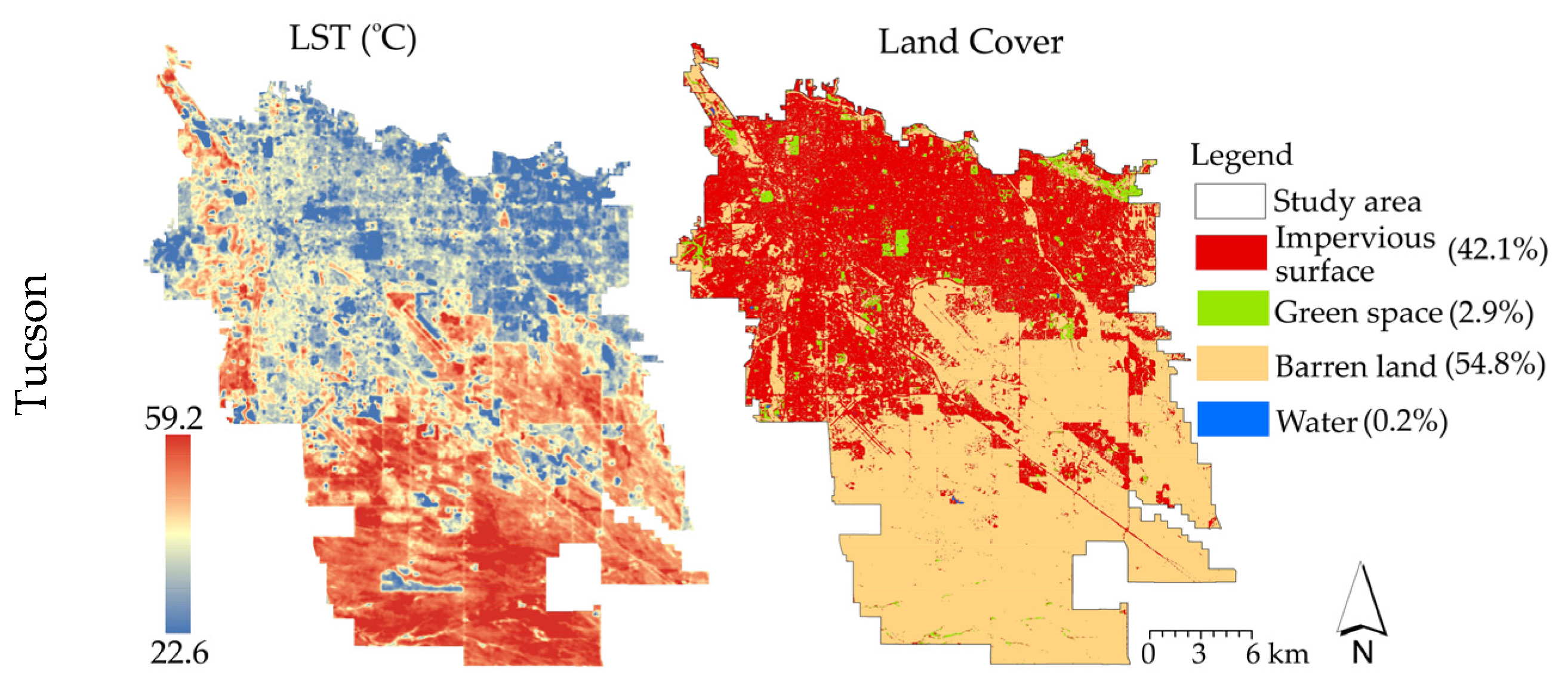
The land cover in the study areas was classified into four distinct types. The classification results yielded an overall accuracy of 90.0% and a Cohen’s kappa coefficient of 0.84 for Phoenix, and 91.6% and 0.85, respectively, for Tucson (

Table 3. Assessment of the accuracy of land cover classification maps.

Classes	Phoenix			Tucson
	PA	UA	FS	PA	UA	FS
Impervious surface	91.18	90.04	90.61	91.44	89.06	90.24
Green space	89.83	91.38	90.60	84.85	87.50	86.15
Barren land	88.71	89.19	88.95	92.91	93.96	93.43
Water	88.24	93.75	90.91	83.33	90.91	86.96
	OA: 90.0%, Kappa: 0.84			OA: 91.6%, Kappa: 0.85

). In Phoenix, the most extensive land cover is impervious surfaces, accounting for 55.4% of the total area, followed by barren land (37.4%), green space (6.8%), and water surfaces (0.4%). In contrast, barren land constitutes the widest land cover type in Tucson, comprising 54.8% of the area, followed by impervious surfaces (42.1%), green space (2.9%), and water surfaces (0.2%) (Figure 3).

In Phoenix, LST ranges from a minimum of 27.5 °C to a maximum of 57.8 °C, with a mean of 49.0 °C ± 2.5 °C. In Tucson, the minimum LST is 22.5 °C, the maximum is 59.2 °C, and the mean is 50.4 °C ± 2.4 °C. An analysis of LST based on landscape composition in Phoenix reveals that impervious surfaces exhibit LST values ranging from 30.9 °C to 57.8 °C, with a mean temperature of 48.9 °C ± 2.1 °C. In green areas, the LST values range from 31.1 °C to 54.0 °C, with a mean of 44.9 °C ± 3.5 °C. Barren lands exhibit LST values from 27.5 °C to 55.1 °C, with a mean of 50.0 °C ± 1.9 °C, while water surfaces indicate LST values between 30.9 °C and 52.9 °C, with a mean of 37.8 °C ± 4.5 °C. In Tucson, impervious surfaces have LST values ranging from 23.6 °C to 59.1 °C, with a mean of 49.0 °C ± 1.6 °C. In green areas, LST ranges from 34.3 °C to 57.7 °C, with a mean of 45.9 °C ± 2.9 °C. Barren lands exhibit LST values between 22.6 °C and 59.2 °C, with a mean of 51.6 °C ± 1.9 °C. Finally, water surfaces in Tucson show LST values ranging from 34.3 °C to 54.8 °C, with a mean temperature of 42.2 °C ± 5.1 °C.

The variation in LST values between the two cities can be attributed to differences in vegetation structure and density, as well as the extent of impervious surfaces. Higher LST values are observed particularly in expansive barren areas characterized by dense urban fabric and limited natural vegetation, which are shaped by the ecological characteristics of the region (Figure 5).

The relationship between mean LST and impervious surface, green space, and barren land at different grid sizes ranging from 3 × 3 to 15 × 15 pixels for the cities of Phoenix and Tucson was evaluated by a correlation analysis. All correlations across different grid sizes were statistically significant (p < 0.001). In both cities, there was a consistently positive correlation between the densities of impervious surfaces and barren land, and the mean LST. However, the correlation between impervious surfaces and mean LST was stronger than that between barren land and mean LST. For both land cover types, the strength of the correlation showed a decreasing trend as grid size increased. In Phoenix, the correlation coefficient for impervious surfaces decreased from 0.86 to 0.74, whereas in Tucson, it declined more moderately, from 0.68 to 0.56. The correlation coefficient for barren land in Phoenix decreased slightly from 0.85 to 0.82, while in Tucson, it decreased from 0.89 to 0.83. The green space density exhibited a statistically significant negative correlation with LST in both cities. In Phoenix, the correlation coefficient increased from −0.74 to −0.87, while in Tucson, it ranged from −0.56 to −0.68 (Figure 6).

The trends of the correlation coefficients between the mean LST and the densities of the identified land covers at different grid sizes intersect at the 9 × 9 grid size. Therefore, mean LST and land cover density maps were created in a 9 × 9 grid size. Accordingly, a linear regression analysis was performed to test the direction, strength, and significance of the relationship between mean LST and land cover density. In both cities, a positive and statistically significant (p < 0.001) relationship was found between the density of impervious surfaces and barren land, and the mean LST value. The slope values of impervious surfaces are 0.1685 in Phoenix (R²: 0.70) and 0.1024 in Tucson (R²: 0.40). The slope values of barren land are 0.1823 (R²: 0.72) in Phoenix and 0.1435 (R²: 0.76) in Tucson. However, a negative and statistically significant (p < 0.001) relationship was observed between green space density and mean LST value in both cities. The slope values of green space are 0.1685 in Phoenix (R²: 0.70) and 0.1025 in Tucson (R²: 0.40) (Figure 7).

UTFVI maps reveal significant differences in the urban thermal patterns of the two cities. In Phoenix, UTFVI values range from −0.438 to 0.178, with a notable concentration of high-index areas in the northern and northeastern regions. Conversely, the central and southern parts of the city exhibit moderate to low UTFVI values. Tucson presents a broader spectrum of thermal conditions, with UTFVI values ranging from −0.552 to 0.176. The southern and southeastern portions of Tucson show noticeably high-index values, suggesting stronger urban heat effects, while the northern and central areas exhibit lower UTFVI values (Figure 8).

The UTFVI values for the cities of Phoenix and Tucson indicate that 42.5% (590.15 km²) of Phoenix and 49.7% (342.95 km²) of Tucson are classified as low SUHI–excellent EEI (UTFVI < 0). A middle SUHI effect (UTFVI: 0.005–0.010) is observed over 4.4% (60.66 km²) of Phoenix and 3.1% (21.32 km²) of Tucson. In the study areas, the strongest SUHI and worst EEI (UTFVI > 0.020) affect 39.8% (552.90 km²) of Phoenix and 37.8% (260.99 km²) of Tucson. Both cities have extensive areas under the effect of high SUHIs (

Table 4. Percentage coverage area of SUHIs and EEI by the threshold of UTFVI.

UTFVI Range	SUHI	EEI	Phoenix		Tucson
			Area (km2)	Percentage (%)	Area (km2)	Percentage (%)
<0	None	Excellent	590.15	42.5	342.95	49.7
0–0.005	Weak	Good	59.90	4.3	22.76	3.3
0.005–0.010	Middle	Normal	60.66	4.4	21.32	3.1
0.010–0.015	Strong	Bad	61.59	4.4	20.96	3.0
0.015–0.020	Stronger	Worse	63.78	4.6	21.22	3.1
>0.020	Strongest	Worst	552.90	39.8	260.99	37.8

).

When the study areas are classified according to LCZ types, Phoenix includes six built types, excluding LCZ 1, LCZ 2, LCZ 5, and LCZ 10, and six land cover types, excluding LCZ A. In Tucson, five built types are present, excluding LCZ 1, LCZ 2, LCZ 4, LCZ 7, and LCZ 10, along with six land cover types, again excluding LCZ A. The most dominant built type in both Phoenix and Tucson is LCZ 6 (open low-rise), accounting for 41.710% and 35.586% of the total area, respectively. Regarding land cover, the most extensive class in Phoenix is LCZ F (bare soil or sand), with 21.124%, while in Tucson, it is LCZ C (bush and scrub), covering 29.769% of the area (

Table 5. Area proportion and mean SUHIs of each LCZs and in Phoenix and Tucson.

LCZs	Phoenix		Tucson		LCZs	Phoenix		Tucson
	Area (%)	SUHI	Area (%)	SUHI		Area (%)	SUHI	Area (%)	SUHI
3: Compact low-rise	0.570	−0.4	0.289	−0.6	B: Scattered trees	0.047	−3.4	0.011	−3.2
4: Open high-rise	0.036	−0.9	-		C: Bush, scrub	12.576	0.3	29.769	0.9
5: Open mid-rise	-		0.005	−3.0	D: Low plants	3.324	−1.8	1.426	−1.1
6: Open low-rise	41.710	−0.1	35.586	−0.7	E: Bare rock or paved	0.591	0.1	0.174	−0.6
7: Lightweight low-rise	0.001	−1.2	-		F: Bare soil or sand	21.124	0.4	14.872	0.2
8: Large low-rise	18.048	0.0	7.617	−0.5	G: Water	0.103	−4.8	0.036	−3.8
9: Sparsely built	1.870	−0.1	10.215	−0.1

). It was found that the LCZ C, LCZ E, and LCZ F zones in Phoenix tend to exhibit a heat island effect with positive SUHI values, while the LCZ 8 zone exhibits neutral thermal behavior. The remaining LCZ zones tend to exhibit a cool island effect with negative SUHI values. Similarly, in Tucson, LCZ C and LCZ F are the zones that increase the urban heat island effect, whereas all other LCZ zones have a cooling effect with lower surface temperatures (Table 5).

The findings reveal that the magnitude of SUHIs in Phoenix and Tucson varies significantly depending on the characteristics of LCZs. A transect-based analysis in Phoenix indicates that the SUHI values range from −5.0 °C to +2 °C, reflecting a wide thermal gradient across the urban landscape. Particularly, positive SUHI values are predominantly observed in LCZ 6, LCZ 9, and LCZ F, indicating that these zones exhibit higher LST than their surroundings. In the LCZ 8 zone, SUHI values fluctuate between positive and negative, generally exhibiting a neutral thermal trend. On the other hand, LCZ 3 areas demonstrate negative SUHI values. Furthermore, zones characterized by natural land cover (LCZ B, LCZ C, and LCZ D) show predominantly negative SUHI values, implying that these areas tend to dissipate rather than retain heat. Among them, LCZ B and LCZ D display strong cooling effects, with SUHI values of −3.6 °C and −3.9 °C, respectively, while LCZ C also contributes to urban cooling, with a SUHI value of −1.4 °C. Additionally, a significant decrease in SUHI magnitude was observed at higher elevations between 21 and 25 km. This reveals that in addition to LCZs, elevation is also an effective factor on SUHI values in desert cities (Figure 9).

A transect-based analysis in Tucson reveals that SUHI magnitudes range from –2.5 °C to +2.0 °C. Notably, the LCZ C and LCZ F zones generally exhibit positive SUHI values, indicating that these areas have higher LST compared to their surroundings and thus demonstrate a pronounced SUHI. In the LCZ 3, LCZ 8, and LCZ 9 zones, SUHI values have both negative and positive values and generally exhibit a neutral thermal pattern. On the other hand, in the LCZ 6, LCZ 8, LCZ 9, LCZ D, and LCZ E zones, SUHI values are negative, and these zones have lower land surface temperature compared to other zones. Specifically, the LCZ 8 and LCZ 9 zones exhibit a cool island effect, with significant negative SUHI values of −1.9 °C and −2.1 °C, respectively. Moreover, a significant decreasing trend in the SUHI magnitude with a steady increase in elevation in the analyzed cross-section was observed (Figure 10).

The landscape composition and structural interactions driving LST variability in Phoenix and Tucson were evaluated using various landscape metrics. The findings reveal that there are significant spatial differences between the two cities. Phoenix has more complex landscape geometry and heterogeneous land cover distribution with high LSI (72.3184) and SHDI (0.8773). In contrast, Tucson exhibits a less complex and heterogeneous landscape structure than Phoenix, with lower LSI (34.0228) and SHDI (0.7947) values. The CONTAG values are medium–high in both cities (Phoenix: 54.1932; Tucson: 61.2376). This indicates that impervious surfaces and barren lands are more dispersed but tend to group together in Phoenix, whereas in Tucson, more extensive and homogeneous barren lands are predominant. The DIVISION metric is significantly higher in Phoenix (0.7427), indicating that green areas are more fragmented and discontinuous than in Tucson (0.6466) (

Table 6. Landscape pattern indices of the study areas at the landscape scale.

City	LSI	CONTAG	DIVISION	SHDI
Phoenix	72.3184	54.1932	0.7427	0.8773
Tucson	34.0228	61.2376	0.6466	0.7947

).

4. Discussion

Increasing temperatures due to global climate change and urbanization are a major climatic risk for ecosystems and societies worldwide. The increase in artificial surfaces (buildings, roads, concrete, and asphalt surfaces) that absorb and emit solar heat with the impact of urbanization increases the severity of UHI because these surfaces absorb solar radiation during the day and re-emit it at night due to the decrease in albedo. Thus, the negative impact of UHI is exacerbated by the increase in LST [62]. Studies show that UHIs cause urban temperatures to be an average of 4 °C higher during the day and 2.5 °C higher at night [95,96]. In the US, temperatures have increased by 1 °C since 1900. However, given global climate change and projected greenhouse gas emissions, temperatures are expected to rise by 6.7 °C until 2100 [97,98].

4.1. Spectral Index and Spatial Resolution

Spectral indices derived from Landsat-9 OLI-2/TIRS-2 satellite imagery were used to create the landscape composition and determine the optimal grid size. Since the creation of all spectral indices from a single satellite image has the potential to cause a multicollinearity problem [99,100,101], the multicollinearity in the created models was queried with the Variance Inflation Factor (VIF). In the literature, it is accepted that a VIF value above 10 indicates multicollinearity in the dataset [102,103,104]. When the multicollinearity of the spectral indices derived from Landsat satellite imagery was investigated, VIF values ranging from 2.2 to 3.9 for Phoenix and 1.4 to 4.7 for Tucson were obtained. Since these VIF values are below 10 in both cities, it is determined that there is no multicollinearity problem in the model.

In the graph obtained as a result of calculating the correlations of the spectral indices derived from Landsat satellite imagery with LST according to different grid sizes, the grid size where the correlation trends intersect is determined as 9 × 9 pixels for both cities. This spatial resolution was found to be the most appropriate scale to be used in LST/SUHI-oriented spatial planning studies in desert cities. The rationale for using different grid sizes at this stage is that, as Athukorala and Murayama [5] point out, an optimal grid size and spatial resolution for urban studies by climate type has not been defined in the literature yet. In this context, there are ongoing studies in the literature to determine the optimal spatial resolution in order to conduct climate-oriented spatial planning studies in regions with different climate types. In the studies carried out in this scope, a 7 × 7 pixel (210 m × 210 m) grid size was used in studies conducted in Bangkok, Jakarta, and Manila in Southeast Asia [28]; in Niğde, Turkey [105]; in Addis Ababa, Ethiopia [62]; and in Tsukuba and Tsuchiura, Japan [106]. In the study conducted in Accra, Ghana, 7 × 7 pixels (210 m × 210 m) and 8 × 8 pixels (240 m × 240 m) grid sizes were used [5]. In the study carried out in Hangzhou, China, grid sizes of 7 × 7 pixels (210 m × 210 m), 15 × 15 pixels (450 m × 450 m), and 23 × 23 pixels (690 m × 690 m) were used [107]. In desert cities, the relationship between land cover and mean LST was found to be statistically significant across various grid sizes ranging from 3 × 3 pixels (90 m × 90 m) to 15 × 15 pixels (450 m × 450 m). In previous studies, spatial resolution is similar in some regions, while in other regions, it differs due to the ecological structures specific to that region.

4.2. The Impact of Landscape Composition on LST

The cities of Phoenix and Tucson are among the hottest cities in the US. In the early 20th century, Tucson was Arizona’s largest city and commercial center, while Phoenix was an agricultural city. However, after Phoenix became the capital of the state of Arizona, the region attracted technology companies following World War II (1950). The widespread adoption of cooling systems, driven by technological advancements, contributed to a rapid population increase and led to the expansion and intensification of urbanization. Nowadays, Phoenix is the fifth most populous city in the US. Due to the impact of urbanization, the minimum average temperatures in the cities of Phoenix and Tucson are 3.8 °C and 1.3 °C higher than the surrounding rural areas, respectively [108,109]. Particularly, the heat vulnerability of neighborhoods within the Phoenix metropolitan area has become a significant concern in recent years [110].

The dominance of impervious surfaces in Phoenix and barren lands in Tucson clearly reflects the differences in landscape composition between the two cities. This structural difference leads to a higher mean surface temperature in Tucson (50.4 °C ± 2.4 °C) compared to Phoenix (49.0 °C ± 2.5 °C). The limited amount of green spaces and water surfaces in both cities shows the determining influence of the arid climatic conditions in the region on the landscape composition. The landscape composition map shows that urban sprawl is a more dominant land cover class in Phoenix than in Tucson. Accordingly, the mean LST measured on impervious surfaces was 49.0 °C ± 1.6 °C in Tucson and 48.9 °C ± 2.1 °C in Phoenix. These findings suggest that urban surfaces tend to have higher temperatures compared to their surroundings and that these structures increase the SUHI effect. According to the landscape composition, barren lands are the most extensive land cover in Tucson. In both Phoenix and Tucson, barren lands have the highest LST values in the landscape composition. Although both cities have similar climatic conditions, the wider, integrated, and denser distribution of desert areas in Tucson caused the LST values in these areas to be 1.6 °C higher than in Phoenix. The results obtained are in line with the findings of previous studies on LST that surface temperature tends to increase as a result of anthropogenic effects in areas with high building density and low vegetation cover [3,15,111,112].

In both cities, the low share of green spaces in the total area reveals that the arid climatic conditions typical of desert cities are effective as a limiting factor in the presence of green spaces. The mean LST values of green spaces were found to be significantly lower than those of impervious surfaces in both cities. The fact that green spaces are more dense and widespread in Phoenix than in Tucson has affected the LST gap between the two cities. In both cities, water surfaces constitute the least extensive land cover class in the landscape composition, while also representing the lowest LST values among all surface classes. Notably, the wider extent of water surfaces in Phoenix ensures that the LST is 4.4 °C lower on average in these areas than in Tucson. However, the limited proportion of water surfaces to total land area in both cities suggests that potential cooling effects are spatially constrained, especially during the hot summer months that characterize these arid desert environments.

Given their location within a desert ecosystem, the cities of Phoenix and Tucson exhibit a higher proportion of areas with high UTFVI values, intense UHI effects, and worse EEI scores compared to regions dominated by other ecosystem types. Increased impervious surfaces due to the rapid urbanization of Phoenix cause these areas to be more extensive than in Tucson. Moreover, high levels of heat island effects are also observed in regions where barren land is the prevailing land cover. Moderate UHI intensities are mostly observed in transitional zones characterized by mixed land use patterns, where green space coverage begins to decline while impervious surfaces and barren land gradually increase. In particular, Tucson has a higher percentage of areas with low UHI impact and high ecological quality than Phoenix. This can be attributed to a combination of factors, including Tucson’s geographical setting, its urban morphological structure, and the comparatively lower prevalence of impervious surfaces. These findings suggest that urban form and planning strategies tailored to local ecological conditions can play a critical role in mitigating UHI effects and promoting environmental sustainability in arid urban environments.

Suburban areas in Phoenix and Tucson have higher LST values during the daytime compared to urban areas. Moreover, the regression analysis between land cover and mean LST in both cities shows that barren land has the highest effect on mean LST in both Phoenix (trend slope: 0.1823, p < 0.001) and Tucson (trend slope: 0.1435, p < 0.001). This appears to be due to the widespread presence of barren land in suburban areas, which mostly absorbs sunlight rather than reflects it, as supported by observational evidence and previous studies [113,114]. Comparable findings have been reported for other arid and semi-arid cities, such as Abu Dhabi, Kuwait City, Riyadh, and Las Vegas, where extensive barren lands in suburban areas lead to higher land surface temperatures during the daytime than in urban areas [113,114,115,116,117].

The SUHI values calculated according to LCZs through cross-sectional analyses in Phoenix and Tucson revealed that landscape composition has a determining effect on surface temperatures in both cities. However, the intensity and spatial distribution of SUHIs varies depending on the urbanization patterns and environmental characteristics of the cities. The SUHI values ranged from −5.0 °C to +1.5 °C in Phoenix and from −2.5 °C to +2.0 °C in Tucson. In both cities, the predominance of positive SUHI values in the desert characterized areas defined by LCZ F indicates that these areas have higher surface temperatures compared to their surroundings. However, in Phoenix, positive SUHI values are observed even in areas such as LCZ 6 and LCZ 9, indicating that these areas are not environmentally supported by adequate cooling green infrastructure. In contrast, the negative SUHI values observed in LCZ 6 in Tucson suggest that the effective integration of natural elements into urban planning enhances the cooling effect. The observation of negative SUHI values in the LCZ 3 zone in both cities shows that dense buildings cannot always be directly associated with high surface temperatures. This can be explained by factors such as the thermal properties of the building materials used, shading ratios, and microclimatic conditions. In Phoenix, the LCZ C and LCZ D land cover types reveal a cooling effect, with significant negative SUHI values ranging from −3.6 °C to −3.9 °C, while in Tucson, similar effects are observed not only in natural areas but also in sparsely built-up zones such as LCZ 8 and LCZ 9. Finally, the decreasing trend in SUHI values with increasing elevation in both cities indicates that topography also plays an important regulatory role in the spatial distribution of SUHI magnitudes.

4.3. Landscape-Based Planning Approach Versus LST

Residential areas and barren land increase the temperature of the thermal environment [118], while forests, agricultural fields, parks, lawns, grasslands, water bodies, and other vegetation patterns within urban landscapes have a significant cooling effect [119,120,121,122,123] because it has been emphasized in academic studies that the high thermal capacity and evaporation effects of these areas reduce the LST and the severity of the SUHI by regulating the regional microclimate [119]. In addition to the presence of urban landscape areas, the spatial configuration of these areas and the built environment has a determining effect on LST [124,125,126]. In particular, the size, form, vegetation cover and type, and spatial distribution of green areas have an impact on the LST value.

Studies show that the SUHI effect increases in landscapes with high LSI and SHDI values, whereas the SUHI effect decreases in landscapes with high CONTAG values [127]. In this study, Phoenix has more fragmented, heterogeneous, and complex landscapes with high DIVISION, SHDI, and LSI values, while the CONTAG value is lower compared to Tucson. This is consistent with the high surface temperatures observed in Phoenix and the pronounced SUHI effect. In Phoenix, fragmented green spaces and complex landscape shapes increase microclimatic diversity but have limited impact on reducing LST due to disconnectedness. The more integrated landscape structure of Tucson can relatively reduce the intensity of SUHIs; however, the low proportion of green space and the extensive presence of barren land (54.8%) is a factor that increases local heat accumulation. These pieces of evidence point to the need for spatial planning strategies that are specific to the local ecological context. In Phoenix, planning green infrastructure in a connected and compact network can increase the cooling effect by reducing fragmentation. In Tucson, the ecological enrichment of barren lands with arid-tolerant vegetation can contribute to reducing surface temperatures by disrupting the compact nature of these areas.

Studies show that the cooling effect of urban green spaces is effective at a distance of 200–400 m around them, depending on the type and spatial configuration of these spaces [126,128,129]. In addition, planning green spaces in a large, well-connected, and continuous structure within the green infrastructure system seems to be more effective in reducing LST value and the severity of UHIs than smaller and fragmented green spaces [130]. However, opportunities to increase the presence of urban landscapes that provide cooling benefits are often constrained by existing land use in cities [23,122]. For instance, the fact that most of the land in Phoenix is owned by the private sector and more than 45% of it is used for residential areas [131] is a limiting factor in the planning and implementation of landscapes [71]. Therefore, optimizing the spatial configuration of landscape compositions is essential to maximize their cooling and ecological benefits.

In arid desert cities, since a large, continuous, clustered green space has a higher cooling effect [132,133], planting trees in urban areas, building rooftop gardens, increasing park areas, and protecting existing water surfaces are necessary to reduce LST and mitigate UHIs in the cities of Phoenix and Tucson. In particular, the limited availability of land for planning green spaces due to dense built-up areas in both urban centers increases the importance of rooftop gardens. Rooftop gardens reduce air temperature at the micro-scale through evapotranspiration and evaporation [134], which will reduce the use of cooling systems and excessive energy demand [36,37]. This will lead to a considerable decrease in the severity of UHIs, especially at night. Moreover, using materials with high albedo, with low heat emission, and that are heat-resistant in structural areas (buildings, impervious surfaces, etc.) and prioritizing energy-efficient building designs are important strategies to mitigate LST and UHI. Meanwhile, Zheng et al. [132] revealed that clustered asphalt surface patterns yielded higher LST than dispersed patterns in their study in Phoenix. Therefore, the integrated structure of large impervious surfaces in both cities should be fragmented by using landscape elements (trees, shrubs, ground covers, mulch, etc.). In addition, the shade of the surrounding buildings should be taken into account during the planning phase to reduce the negative thermal impact of these large impervious surfaces and to provide a cooling effect.

Trees in arid desert cities have a stronger cooling effect than grass and shrubs [49]. The master plan prepared by the City of Phoenix in 2010 to reduce UHI in the city aims to increase tree cover from 10% to 25% [135]. Middel et al. [22] showed that increasing tree cover from 10% to 25% according to this master plan would lead to a 2 °C temperature reduction at the local scale. However, even a 25% increase in tree cover would not be enough to mitigate the increased heat caused by climate change [22]. The City of Tucson’s “The Tucson Million Trees” initiative plans to plant one million trees by 2030 to increase tree cover in the city and tackle climate change [136]. Moreover, the strategic configuration of trees (location, arrangement, density, etc.) will also play an important role in enhancing the cooling effect provided by trees at the micro-scale.

Studies in desert cities have shown a positive correlation between social vulnerability (homeless, low-income individuals, elderly, sick, etc.) and LST/UHIs [137,138,139]. Therefore, it has been determined that green space density is low and LST/UHIs and thermal discomfort are high in areas with high social vulnerability. Moreover, it is emphasized in studies that increasing UHIs and high temperatures due to urbanization in arid desert regions may cause an increase in heat-related mortality rates in areas where socially vulnerable populations live densely [76,140]. In Phoenix and Tucson, green spaces planned for neighborhoods with high social vulnerability will provide spatial cooling through both shading and evapotranspiration, reduce the urban UHI impact, and increase thermal comfort by reducing heat stress caused by UHIs.

In arid desert cities, a balanced landscape planning approach is important because water resources are scarce and land use areas for landscaping are limited. Particularly during summer periods of extreme heat, a certain proportion of water resources is used for the irrigation of green areas/vegetation that provide spatial cooling through shading and evaporation, reducing urban UHIs and increasing thermal comfort [141]. This causes concerns about water management in desert cities due to the economic cost to local governments and the impact on the ecological structure [142,143,144]. Preferring the arid landscape (xeriscape) approach [145,146] and using arid-tolerant tree species (low-water-use trees) in landscape applications in arid desert cities instead of traditional and common landscape applications in regions with different climate types will contribute significantly to both the cooling effect and water saving. In this context, the preference for desert-adapted tree species such as Catclaw acacia (Acacia greggii), Blue palo verde (Parkinsonia florida), Desert ironwood (Olneya tesota), Desert willow (Chilopsis linearis), Velvet mesquite (Prosopis velutina), and Foothill palo verde (Parkinsonia microphylla) in Phoenix and Tucson will increase this contribution.

Although Phoenix and Tucson do not receive excessive annual precipitation, sudden heavy rainfall, especially during the monsoon season due to climate change, can cause flash floods. One of the main causes of these flash floods is the increase in impervious surfaces resulting from urbanization. Impervious surfaces lead to stormwater surface runoff, reduced water quality, and the inability to recharge groundwater resources. However, using permeable surfaces in urban applications (permeable concrete materials, green areas, and soil surfaces) will contribute to controlling rainwater runoff, recharging groundwater resources, and reducing temperatures [71,147]. This is because the radiant heat from pervious concrete surfaces is lower than that from impervious concrete surfaces, which is effective in reducing the temperature [148].

4.4. Limitations of This Study

Landsat-9 satellite imagery, which is publicly available from USGS, was used for the analysis in this study. The fact that these satellite images are of a certain time interval, belong to daytime hours, and have a certain medium resolution determines the level of detail of the study. In particular, these satellite images are insufficient for the detailed identification of land uses and covers in a heterogeneous urban environment at high resolution. Therefore, it was impossible to determine the impact of each land cover type, such as each building or tree, on the LST and SUHIs in cities separately. Moreover, studies in arid desert cities have shown that asphalt/impervious surfaces increase LST both day and night [49]. However, since Landsat satellites acquire data during the daytime in this region, the nighttime effect of land use/cover on LST could not be evaluated.

To evaluate the impact of landscape composition on LST in Phoenix and Tucson, analyses were performed with satellite imagery from July, when LST reaches the highest levels and the SUHI effect is most clearly observable. However, in future studies, the impact of seasonal variations should be revealed by using multi-temporal satellite images (different seasons and years), and the stability of the findings over time should be tested.

In future studies, using satellite imagery with very high resolutions and different time intervals (day/night) will enable a more detailed assessment of the individual impacts of land use/cover and landscape composition/configuration on LST and SUHIs. In the analyses performed via satellite imagery, the effect of objects (buildings, trees, etc.) was evaluated in the horizontal plane. Therefore, the climatic features created by trees and other tall objects on vertical surfaces could not be assessed. It is suggested that future similar studies consider the effect of trees or other structural elements on vertical surfaces.

5. Conclusions

The SUHI effect in arid desert cities such as Phoenix and Tucson, particularly intensified during the summer due to extreme temperatures, has significant social and economic impacts on local communities. Increased energy consumption in response to extreme temperatures, increased water use in housing and green spaces, and health risks for vulnerable social groups further increase the importance of urban planning in these cities. Therefore, effective adaptation strategies and holistic urban plans are essential to mitigate the challenges of regional climate conditions in arid desert cities.

Strategies for spatially integrated planning and design of green spaces and impervious surfaces in the cities of Phoenix and Tucson should be developed to reduce LST and mitigate SUHI severity, provide sustainable ecosystem services, and increase urban thermal comfort because only structural measures will not be sufficient to deal with the potential negative impacts of climate change. Accordingly, it is of great importance to create urban wind corridors, plan rooftop gardens, increase water bodies, use materials with low heat absorption capacity in buildings, increase green areas, and develop a regional green infrastructure system, especially with drought-resistant plant species.

This study contributes to the literature by revealing the effects of urban landscape composition on LST and SUHI impact in arid desert cities. In this study, a multi-resolution grid-based analysis revealed that a spatial resolution of 9 × 9 pixels is optimal for assessing the impact of landscape composition on LST in arid desert cities such as Phoenix and Tucson. The landscape composition analysis showed that both cities have fragmented green spaces, along with complex landscape geometry and heterogeneous land cover distribution. However, the predominance of impervious surfaces in Phoenix and desert areas in Tucson clearly revealed differences in landscape composition between the cities. These compositional variations significantly affected the LST values observed in both cities. Moreover, the SUHI values calculated according to LCZs confirmed that landscape composition is a determining factor on surface temperatures. Overall, these results emphasize the importance of considering landscape composition and structure in climate-oriented spatial planning studies.

The results of this study provide guidance for planners, designers, and decision-makers who are developing strategies and plans to reduce high LST values and SUHI impact in these cities. Moreover, tackling LST in cities should not be limited to the work of decision-makers and planners, while developing strategies and planning scenarios, analyzing the socio-economic and socio-cultural structure of the city, evaluating socio-spatial interactions, and considering engineering solutions and nature-based solutions with a holistic planning paradigm will be effective in creating sustainable, resilient, and livable cities.

References

1. Cook, J.; Nuccitelli, D.; Green, S.A.; Richardson, M.; Winkler, B.; Painting, R.; Way, R.; Jacobs, P.; Skuce, A. Quantifying the consensus on anthropogenic global warming in the scientific literature. Environ. Res. Lett. 2013, 8, 024024. [Google Scholar] [CrossRef]
2. NASA. Available online: https://science.nasa.gov/climate-change/causes/ (accessed on 12 January 2025).
3. Sarif, M.O.; Rimal, B.; Stork, N.E. Assessment of changes in land use/land cover and land surface temperatures and their impact on surface urban heat island phenomena in the Kathmandu Valley (1988–2018). ISPRS Int. J. Geo-Inf. 2020, 9, 726. [Google Scholar] [CrossRef]
4. Koko, A.F.; Yue, W.; Abubakar, G.A.; Alabsi, A.A.N.; Hamed, R. Spatiotemporal influence of land use/land cover change dynamics on surface urban heat island: A case study of Abuja Metropolis, Nigeria. ISPRS Int. J. Geo-Inf. 2021, 10, 272. [Google Scholar] [CrossRef]
5. Athukorala, D.; Murayama, Y. Spatial variation of land use/cover composition and impact on surface urban heat island in a tropical sub-saharan City of Accra, Ghana. Sustainability 2020, 12, 7953. [Google Scholar] [CrossRef]
6. Venkatraman, S.; Kandasamy, V.; Rajalakshmi, J.; Sabarunisha, B.S.; Sujatha, M. Assessment of urban heat island using remote sensing and geospatial application: A case study in Sao Paulo city, Brazil, South America. J. S. Am. Earth Sci. 2024, 134, 104763. [Google Scholar]
7. Tan, P.Y.; Zhang, J.; Masoudi, M.; Alemu, J.B.; Edwards, P.J.; Grêt-Regamey, A.; Richards, D.R.; Saunders, J.; Song, X.P.; Wong, L.W. A conceptual framework to untangle the concept of urban ecosystem services. Landsc. Urban Plan. 2020, 200, 103837. [Google Scholar] [CrossRef]
8. Guha, S.; Govil, H.; Gill, N.; Dey, A. Analytical study on the relationship between land surface temperature and land use/land cover indices. Ann. GIS 2020, 26, 201–216. [Google Scholar] [CrossRef]
9. Azevedo, J.A.; Chapman, L.; Muller, C.L. Quantifying the daytime and night-Time urban heat island in Birmingham, UK: A comparison of satellite derived land surface temperature and high resolution air temperature observations. Remote Sens. 2016, 8, 153. [Google Scholar] [CrossRef]
10. Min, M.; Zhao, H.; Miao, C. Spatio-Temporal evolution analysis of the urban heat island: A case study of Zhengzhou City, China. Sustainability 2018, 10, 1992. [Google Scholar] [CrossRef]
11. Gohain, K.J.; Mohammad, P.; Goswami, A. Assessing the impact of land use land cover changes on land surface temperature over Pune city, India. Quat. Int. 2021, 575–576, 259–269. [Google Scholar] [CrossRef]
12. Naim, M.N.H.; Kafy, A.A. Assessment of urban thermal field variance index and defining the relationship between land cover and surface temperature in Chattogram city: A remote sensing and statistical approach. Environ. Chall. 2021, 4, 100107. [Google Scholar] [CrossRef]
13. NASA. Available online: https://landsat.gsfc.nasa.gov/ (accessed on 19 December 2024).
14. Gomez-Martinez, F.; de Beurs, K.M.; Koch, J.; Widener, J. Multi-Temporal land surface temperature and vegetation greenness in urban green spaces of Puebla, Mexico. Land 2021, 10, 155. [Google Scholar] [CrossRef]
15. Ranagalage, M.; Ratnayake, S.S.; Dissanayake, D.; Kumar, L.; Wickremasinghe, H.; Vidanagama, J.; Cho, H.; Udagedara, S.; Jha, K.K.; Simwanda, M.; et al. Spatiotemporal variation of urban heat islands for implementing nature-Based solutions: A case study of Kurunegala, Sri Lanka. ISPRS Int. J. Geo-Inf. 2020, 9, 461. [Google Scholar] [CrossRef]
16. Chen, W.; Zhang, Y.; Pengwang, C.; Gao, W. Evaluation of urbanization dynamics and its impacts on surface heat islands: A case study of Beijing, China. Remote Sens. 2017, 9, 453. [Google Scholar] [CrossRef]
17. Masoudi, M.; Tan, P.Y. Multi-Year comparison of the effects of spatial pattern of urban green spaces on urban land surface temperature. Landsc. Urban Plan. 2019, 184, 44–58. [Google Scholar] [CrossRef]
18. Choudhury, U.; Singh, S.K.; Kumar, A.; Meraj, G.; Kumar, P.; Kanga, S. Assessing Land use/land cover changes and urban heat island intensification: A case study of Kamrup metropolitan district, Northeast India (2000–2032). Earth 2023, 4, 503–521. [Google Scholar] [CrossRef]
19. Dadashpoor, H.; Khaleghinia, A.; Shabrang, A. Explaining the role of land use changes on land surface temperature in an arid and semi-Arid metropolitan area with multi-Scale spatial regression analysis. Environ. Monit. Assess. 2024, 196, 124. [Google Scholar] [CrossRef]
20. Debbage, N.; Shepherd, J.M. The urban heat island effect and city contiguity. Comput. Environ. Urban Syst. 2015, 54, 181–194. [Google Scholar] [CrossRef]
21. Šalkovič, M.; Pauditšová, E. Use of Satellite Images to determine the temperature of urban surfaces for landscape management purposes, case study Bratislava (Slovak Republic). Land 2023, 12, 384. [Google Scholar] [CrossRef]
22. Middel, A.; Chhetri, N.; Quay, R. Urban forestry and cool roofs: Assessment of heat mitigation strategies in Phoenix residential neighborhoods. Urban For. Urban Green. 2015, 14, 178–186. [Google Scholar] [CrossRef]
23. Hazarika, A.; Saikia, J.; Saikia, S. Evaluating the scenario of urban Blue-Green space in Tezpur town of Assam using Geo-Technical approach. Acta Geophys. 2024, 73, 901–915. [Google Scholar] [CrossRef]
24. Voogt, J.; Oke, T. Thermal remote sensing of urban climates. Remote Sens. Environ. 2003, 86, 370–384. [Google Scholar] [CrossRef]
25. Yuan, F.; Bauer, M.E. Comparison of impervious surface area and normalized difference vegetation index as indicators of surface urban heat island effects in Landsat imagery. Remote Sens. Environ. 2007, 106, 375–386. [Google Scholar] [CrossRef]
26. Hu, Y.; Hou, M.; Jia, G.; Zhao, C.; Zhen, X.; Xu, Y. Comparison of surface and canopy urban heat islands within megacities of eastern China. ISPRS J. Photogramm. Remote Sens. 2019, 156, 160–168. [Google Scholar] [CrossRef]
27. Kalogeropoulos, G.; Tzortzi, J.; Dimoudi, A. Remote Sensing and Field Measurements for the Analysis of the Thermal Environment in the “Bosco Verticale” Area in Milan City. Land 2024, 13, 182. [Google Scholar] [CrossRef]
28. Estoque, R.C.; Murayama, Y.; Myint, S.W. Effects of landscape composition and pattern on land surface temperature: An urban heat island study in the megacities of Southeast Asia. Sci. Total Environ. 2017, 577, 349–359. [Google Scholar] [CrossRef]
29. Zhang, Y.; Wang, Y.; Ding, N.; Yang, X. Spatial pattern impact of impervious surface density on urban heat island effect: A case study in Xuzhou, China. Land 2022, 11, 2135. [Google Scholar] [CrossRef]
30. Cilek, M.U.; Cilek, A. Analyses of land surface temperature (LST) variability among local climate zones (LCZs) comparing Landsat-8 and ENVI-met model data. Sustain. Cities Soc. 2021, 69, 102877. [Google Scholar] [CrossRef]
31. Peng, W.; Wang, R.; Duan, J.; Gao, W.; Fan, Z. Surface and canopy urban heat islands: Does urban morphology result in the spatiotemporal differences? Urban Clim. 2022, 42, 101136. [Google Scholar] [CrossRef]
32. Baik, J.J.; Kim, Y.H.; Kim, J.J.; Han, J.Y. Effects of boundary-Layer stability on urban heat island-Induced circulation. Theor. Appl. Climatol. 2007, 89, 73–81. [Google Scholar] [CrossRef]
33. Coseo, P.; Larsen, L. How factors of land use/land cover, building configuration, and adjacent heat sources and sinks explain Urban Heat Islands in Chicago. Landsc. Urban Plan. 2014, 125, 117–129. [Google Scholar] [CrossRef]
34. Kong, F.; Yin, H.; James, P.; Hutyra, L.R.; He, H.S. Effects of spatial pattern of greenspace on urban cooling in a large metropolitan area of eastern China. Landsc. Urban Plan. 2014, 128, 35–47. [Google Scholar] [CrossRef]
35. Equere, V.; Mirzaei, P.A.; Riffat, S.; Wang, Y. Integration of topological aspect of city terrains to predict the spatial distribution of urban heat island using GIS and ANN. Sustain. Cities Soc. 2021, 69, 102825. [Google Scholar] [CrossRef]
36. Mirzaei, P.A.; Haghighat, F. Approaches to study urban heat island—Abilities and limitations. Build. Environ. 2010, 45, 2192–2201. [Google Scholar] [CrossRef]
37. Osborne, P.E.; Alvares-Sanches, T. Quantifying how landscape composition and configuration affect urban land surface temperatures using machine learning and neutral landscapes. Comput. Environ. Urban Syst. 2019, 76, 80–90. [Google Scholar] [CrossRef]
38. Zhang, L.; Shi, X.; Chang, Q. Exploring adaptive UHI mitigation solutions by spatial heterogeneity of land surface temperature and its relationship to urban morphology in historical downtown blocks, Beijing. Land 2022, 11, 544. [Google Scholar] [CrossRef]
39. Stewart, I.D.; Oke, T.R. Local Climate Zones for Urban Temperature Studies. Bull. Am. Meteorol. Soc. 2012, 93, 1879–1900. [Google Scholar] [CrossRef]
40. Demuzere, M.; Hankey, S.; Mills, G.; Zhang, W.; Lu, T.; Bechtel, B. Combining expert and crowd-sourced training data to map urban form and functions for the continental US. Nat. Sci. Data 2020, 7, 264. [Google Scholar] [CrossRef]
41. Demuzere, M.; Kittner, J.; Martilli, A.; Mills, G.; Moede, C.; Stewart, I.D.; van Vliet, J.; Bechtel, B. A global map of local climate zones to support earth system modelling and urban-Scale environmental science. Earth Syst. Sci. Data. 2022, 14, 3835–3873. [Google Scholar] [CrossRef]
42. Muhammad, F.; Xie, C.K.; Vogel, J.; Afshari, A. Inference of Local Climate Zones from GIS Data, and Comparison to WUDAPT Classification and Custom-Fit Clusters. Land 2022, 11, 747. [Google Scholar] [CrossRef]
43. Abougendia, S.M. Investigating surface UHI using local climate zones (LCZs), the case study of Cairo’s River Islands. Alex. Eng. J. 2023, 77, 293–307. [Google Scholar] [CrossRef]
44. He, X.; Yuan, Q.; Qin, Y.; Lu, J.; Li, G. Analysis of Surface Urban Heat Island in the Guangzhou-Foshan Metropolitan Area Based on Local Climate Zones. Land 2024, 13, 1626. [Google Scholar] [CrossRef]
45. Alexander, P.J.; Mills, G. Local Climate Classification and Dublin’s Urban Heat Island. Atmosphere 2014, 5, 755–774. [Google Scholar] [CrossRef]
46. Estoque, R.C.; Murayama, Y. Classification and change detection of built-up lands from Landsat-7 ETM+ and Landsat-8 OLI/TIRS imageries: A comparative assessment of various spectral indices. Ecol. Indic. 2015, 56, 205–217. [Google Scholar] [CrossRef]
47. Laonamsai, J.; Julphunthong, P.; Saprathet, T.; Kimmany, B.; Ganchanasuragit, T.; Chomcheawchan, P.; Tomun, N. Utilizing NDWI, MNDWI, SAVI, WRI, and AWEI for estimating erosion and deposition in Ping River in Thailand. Hydrology 2023, 10, 70. [Google Scholar] [CrossRef]
48. Rasul, A.; Balzter, H.; Ibrahim, G.R.F.; Hameed, H.M.; Wheeler, J.; Adamu, B.; Ibrahim, S.; Najmaddin, P.M. Applying built-up and bare-soil indices from Landsat 8 to cities in dry climates. Land 2018, 7, 81. [Google Scholar] [CrossRef]
49. Myint, S.W.; Wentz, E.A.; Brazel, A.J.; Quattrochi, D.A. The impact of distinct anthropogenic and vegetation features on urban warming. Landsc. Ecol. 2013, 28, 959–978. [Google Scholar] [CrossRef]
50. Zhuang, Q.; Wu, S.; Yan, Y.; Niu, Y.; Yang, F.; Xie, C. Monitoring land surface thermal environments under the background of landscape patterns in arid regions: A case study in Aksu river basin. Sci. Total Environ. 2020, 710, 136336. [Google Scholar] [CrossRef]
51. Majumder, A.; Setia, R.; Kingra, P.K.; Sembh, H.; Singh, S.P.; Pateriya, B. Estimation of land surface temperature using different retrieval methods for studying the spatiotemporal variations of surface urban heat and cold islands in Indian Punjab. Environ. Dev. Sustain. 2021, 23, 15921–15942. [Google Scholar] [CrossRef]
52. Halder, B.; Karimi, A.; Mohammad, P.; Bandyopadhyay, J.; Brown, R.D.; Yaseen, Z.M. Investigating the relationship between land alteration and the urban heat island of Seville city using multi-Temporal Landsat data. Theor. Appl. Climatol. 2022, 150, 613–635. [Google Scholar] [CrossRef]
53. Sandoval, S.; Escobar-Flores, J.G.; Badar Munir, M. Urbanization and its impacts on land surface temperature and sea surface temperature in a tourist region in Mexico from 1990 to 2020. Remote Sens. Appl. Soc. Environ. 2023, 32, 101046. [Google Scholar] [CrossRef]
54. Moazzam, M.F.U.; Lee, B.G. Urbanization influenced SUHI of 41 megacities of the world using big geospatial data assisted with Google Earth Engine. Sustain. Cities Soc. 2024, 101, 105095. [Google Scholar] [CrossRef]
55. Zhou, W.; Qian, Y.; Li, X.; Li, W.; Han, L. Relationships between land cover and the surface urban heat island: Seasonal variability and effects of spatial and thematic resolution of land cover data on predicting land surface temperatures. Landsc. Ecol. 2014, 29, 153–167. [Google Scholar] [CrossRef]
56. Zhou, W.; Huang, G.; Cadenasso, M.L. Does spatial configuration matter? Understanding the effects of land cover pattern on land surface temperature in urban landscapes. Landsc. Urban Plan. 2011, 102, 54–63. [Google Scholar] [CrossRef]
57. Şahin, M.T.; Hadimli, H.; Çakır, Ç.; Yasak, Ü.; Genişyürek, F. The Role of Urban Landscape on Land Surface Temperature: The Case of Muratpaşa, Antalya. Land 2025, 14, 663. [Google Scholar] [CrossRef]
58. Climas. Understanding Urban Heat Vulnerability and the need for Resilient Design Practice. Available online: https://climas.arizona.edu/news/understanding-urban-heat-vulnerability-and-need-resilient-design-practice (accessed on 22 May 2025).
59. Wu, Q.; Tan, J.; Guo, F.; Li, H.; Chen, S. Multi-Scale Relationship between Land Surface Temperature and Landscape Pattern Based on Wavelet Coherence: The Case of Metropolitan Beijing, China. Remote Sens. 2019, 11, 3021. [Google Scholar] [CrossRef]
60. McGarigal, K.; Cushman, S.A.; Ene, E. FRAGSTATS v4: Spatial Pattern Analysis Program for Categorical Maps. Computer Software Program Produced by the Authors. 2023. Available online: https://www.fragstats.org (accessed on 22 May 2025).
61. Simwanda, M.; Ranagalage, M.; Estoque, R.C.; Murayama, Y. Spatial analysis of surface urban heat islands in four rapidly growing African cities. Remote Sens. 2019, 11, 1645. [Google Scholar] [CrossRef]
62. Dissanayake, D.; Morimoto, T.; Murayama, Y.; Ranagalage, M. Impact of landscape structure on the variation of land surface temperature in Sub-Saharan Region: A case study of Addis Ababa using landsat data (1986–2016). Sustainability 2019, 11, 2257. [Google Scholar] [CrossRef]
63. Shindell, D.; Zhang, Y.; Scott, M.; Ru, M.; Stark, K.; Ebi, K.L. The effects of heat exposure on human mortality throughout the United States. GeoHealth 2020, 4, e2019GH000234. [Google Scholar] [CrossRef]
64. Keith, L.; Meerow, S.; Jensen, L.; Trego, S.; Schmidt, E.L.; Berke, P. Evaluating urban heat mitigation across networks of plans. J. Plan. Educ. Res. 2025, 45, 427–440. [Google Scholar] [CrossRef]
65. Georgescu, M.; Moustaoui, M.; Mahalov, A.; Dudhia, J. Summer-time climate impacts of projected megapolitan expansion in Arizona. Nat. Clim. Change 2012, 3, 37–41. [Google Scholar] [CrossRef]
66. Garfin, G.; Jardine, A.; Merideth, R.; Black, M.; LeRoy, S. Assessment of Climate Change in the Southwest United States: A Report Prepared for the National Climate Assessment, 1st ed.; Island Press: Washington, DC, USA, 2013; pp. 1–506. [Google Scholar]
67. Iwaniec, D.M.; Cook, E.M.; Davidson, M.J.; Berbés-Blázquez, M.; Georgescu, M.; Krayenhoff, E.S.; Middel, A.; Sampson, D.A.; Grimm, N.B. The co-Production of sustainable future scenarios. Landsc. Urban Plan. 2020, 197, 103744. [Google Scholar] [CrossRef]
68. Arizona State Climate Office. Available online: https://azclimate.asu.edu/ (accessed on 14 October 2024).
69. Latitude and Longitude Finder. Available online: https://www.latlong.net/ (accessed on 26 October 2024).
70. Helmrich, A.; Kuhn, A.; Roque, A.; Santibanez, A.; Kim, Y.; Grimm, N.B.; Chester, M. Interdependence of Social-Ecological-Technological systems in Phoenix, Arizona: Consequences of an extreme precipitation event. J. Infrastruct. Preserv. Resil. 2023, 4, 19. [Google Scholar] [CrossRef] [PubMed]
71. Olgun, R.; Cheng, C.; Coseo, P. Nature-Based solutions scenario planning for climate change adaptation in arid and semi-arid regions. Land 2024, 13, 1464. [Google Scholar] [CrossRef]
72. Wikipedia. Available online: https://en.wikipedia.org/wiki/Phoenix,_Arizona (accessed on 3 October 2024).
73. Census Demographic and Housing Characteristics File. 2020. Available online: https://data.census.gov/ (accessed on 7 July 2024).
74. Wikipedia. Available online: https://en.wikipedia.org/wiki/Tucson,_Arizona (accessed on 4 October 2024).
75. NWS. Annual and Monthly Record data for Phoenix. Available online: https://www.weather.gov/psr/ (accessed on 15 September 2024).
76. Johnson, D.P.; Wilson, J.S. The socio-Spatial dynamics of extreme urban heat events: The case of heat-Related deaths in Philadelphia. Appl. Geogr. 2009, 29, 419–434. [Google Scholar] [CrossRef]
77. Azizi, S.; Azizi, T. Urban climate dynamics: Analyzing the impact of green cover and air pollution on land surface temperature-a comparative study across Chicago, San Francisco, and Phoenix, USA. Atmosphere 2024, 15, 917. [Google Scholar] [CrossRef]
78. Kane, K.; Connors, J.P.; Galletti, C.S. Beyond fragmentation at the fringe: A path-Dependent, high-Resolution analysis of urban land cover in Phoenix, Arizona. Appl. Geogr. 2014, 52, 123–134. [Google Scholar] [CrossRef]
79. Cilek, A.; Unal, M.; Middel, A. The effects of 2-D and 3-D urban landscape metrics on mean radiant temperature in hot-arid Phoenix and Tempe, Arizona, USA. Sustain. Cities Soc. 2024, 101, 105116. [Google Scholar] [CrossRef]
80. Suchy, A.K.; Palta, M.M.; Stromberg, J.C.; Childers, D.L. High potential nitrate removal by urban accidental wetlands in a desert city: Limitations and spatiotemporal patterns. Ecosystems 2020, 23, 1227–1242. [Google Scholar] [CrossRef]
81. USGS. Available online: https://www.usgs.gov/ (accessed on 10 October 2024).
82. Abir, F.A.; Ahmmed, S.; Sarker, S.H.; Fahim, A.U. Thermal and ecological assessment based on land surface temperature and quantifying multivariate controlling factors in Bogura, Bangladesh. Heliyon 2021, 7, e08012. [Google Scholar] [CrossRef]
83. Haashemi, S.; Weng, Q.; Darvishi, A.; Alavipanah, S.K. Seasonal variations of the surface urban heat island in a semi-Arid city. Remote Sens. 2016, 8, 352. [Google Scholar] [CrossRef]
84. Kafy, A.A.; Rahman, M.S.; Islam, M.; Rakib, A.A.; Islam, M.A.; Khan, M.H.H.; Sikdar, M.S.; Sarker, M.H.S.; Mawa, J.; Sattar, G.S. Prediction of seasonal urban thermal field variance index using machine learning algorithms in Cumilla, Bangladesh. Sustain. Cities Soc. 2021, 64, 102542. [Google Scholar] [CrossRef]
85. Clinton, N.; Gong, P. MODIS detected surface urban heat islands and sinks: Global locations and controls. Remote Sens. Environ. 2013, 134, 294–304. [Google Scholar] [CrossRef]
86. Shi, Z.; Li, X.; Hu, T.; Yuan, B.; Yin, P.; Jiang, D. Modeling the intensity of surface urban heat island based on the impervious surface area. Urban Clim. 2023, 49, 101529. [Google Scholar] [CrossRef]
87. Olgun, R.; Cheng, C.; Coseo, P. Desert urban ecology: Urban forest, climate, and ecosystem services. Environ. Dev. Sustain. 2024. [Google Scholar] [CrossRef]
88. Liu, L.; Zhang, Y. Urban heat island analysis using the landsat tm data and aster data: A case study in Hong Kong. Remote Sens. 2011, 3, 1535–1552. [Google Scholar] [CrossRef]
89. Singh, P.; Kikon, N.; Verma, P. Impact of land use change and urbanization on urban heat island in Lucknow city, Central India. A remote sensing based estimate. Sustain. Cities Soc. 2017, 32, 100–114. [Google Scholar] [CrossRef]
90. Xu, H. Modification of normalised difference water index (NDWI) to enhance open water features in remotely sensed imagery. Int. J. Remote Sens. 2006, 27, 3025–3033. [Google Scholar] [CrossRef]
91. Li, W.; Du, Z.; Ling, F.; Zhou, D.; Wang, H.; Gui, Y.; Sun, B.; Zhang, X. A comparison of land surface water mapping using the normalized difference water index from TM, ETM+ and ALI. Remote Sens. 2013, 5, 5530–5549. [Google Scholar] [CrossRef]
92. Konapala, G.; Kumar, S.V.; Ahmad, S.K. Exploring Sentinel-1 and Sentinel-2 diversity for flood inundation mapping using deep learning. ISPRS J. Photogramm. Remote Sens. 2021, 180, 163–173. [Google Scholar] [CrossRef]
93. Panahi, H.; Azizi, Z.; Kiadaliri, H.; Almodaresi, S.A.; Aghamohamadi, H. Bare soil detecting algorithms in western Iran woodlands using remote sensing. Smart Agric. Technol. 2024, 7, 100429. [Google Scholar] [CrossRef]
94. Demuzere, M.; Kittner, J.; Martilli, A.; Mills, G.; Moede, C.; Stewart, I.D.; Vliet, J.; Bechtel, B. Global Map of Local Climate Zones (3.0.0). Zenodo. 2023. Available online: https://zenodo.org/records/8419340 (accessed on 20 May 2025).
95. Hibbard, K.A.; Hoffman, F.M.; Huntzinger, D.; West, T.O. Changes in land cover and terrestrial biogeochemistry. In Climate Science Special Report: Fourth National Climate Assessment, 1st ed.; Wuebbles, D.J., Fahey, D.W., Hibbard, K.A., Dokken, D.J., Stewart, B.C., Maycock, T.K., Eds.; U.S. Global Change Research Program: Washington, DC, USA, 2017; Volume 1, pp. 277–302. [Google Scholar]
96. Keith, L.; Meerow, S. Planning for Urban Heat Resilience; PAS Report 600; American Planning Association: Chicago, IL, USA, 2022; Available online: https://planning-org-uploaded-media.s3.amazonaws.com/publication/download_pdf/PAS-Report-600-r1.pdf (accessed on 11 March 2024).
97. Hayhoe, K.; Wuebbles, D.J.; Easterling, D.R.; Fahey, D.W.; Doherty, S.; Kossin, J.P.; Sweet, W.V.; Vose, R.S.; Wehner, M.F. Our changing climate. In Impacts, Risks, and Adaptation in the United States: Fourth National Climate Assessment, 1st ed.; Reidmiller, D.R., Avery, C.W., Easterling, D.R., Kunkel, K.E., Lewis, K.L.M., Maycock, T.K., Stewart, B.C., Eds.; U.S. Global Change Research Program: Washington, DC, USA, 2018; Volume 2, pp. 72–144. [Google Scholar]
98. Crisman, J.J.; Keith, L.; Sami, I.; Garfin, G. Designing chill city: An interactive game supporting public learning about urban planning for extreme heat. J. Environ. Educ. 2023, 54, 225–239. [Google Scholar] [CrossRef]
99. Arbia, G.; Griffith, D.A.; Haining, R.P. Spatial error propagation when computing linear combinations of spectral bands: The case of vegetation indices. Environ. Ecol. Stat. 2003, 10, 375–396. [Google Scholar] [CrossRef]
100. Shahtahmassebi, A.R.; Lin, Y.; Lin, L.; Atkinson, P.M.; Moore, N.; Wang, K.; He, S.; Huang, L.; Wu, J.; Shen, Z.; et al. Reconstructing Historical Land Cover Type and Complexity by Synergistic Use of Landsat Multispectral Scanner and CORONA. Remote Sens. 2017, 9, 682. [Google Scholar] [CrossRef]
101. Efeizomor, R.O. A Comparative Study of Methods of Remedying Multicolinearity. Am. J. Theor. Appl. Stat. 2023, 12, 87–91. [Google Scholar]
102. El-Dereny, M.; Rashwan, N.I. Solving multicollinearity problem using ridge regression models. Int. J. Contemp. Math. Sci. 2011, 6, 585–600. [Google Scholar]
103. Yu, Z.; Di, L.; Yang, R.; Tang, J.; Lin, L.; Zhang, C.; Rahman, M.S.; Zhao, H.; Gaigalas, J.; Yu, E.G.; et al. Selection of Landsat 8 OLI band combinations for land use and land cover classification. In Proceedings of the 8th International Conference on Agro-Geoinformatics (Agro-Geoinformatics), Istanbul, Turkey, 16–19 July 2019; pp. 1–5. [Google Scholar] [CrossRef]
104. Owoyemi, Q.A.; Bolakale, A. Comparative analysis of some linear predictive models in the presence of multicollinearity. Int. J. Adv. Stat. Probab. 2024, 11, 20–28. [Google Scholar]
105. Soydan, O. Effects of landscape composition and patterns on land surface temperature: Urban heat island case study for Nigde, Turkey. Urban Clim. 2020, 34, 100688. [Google Scholar] [CrossRef]
106. Ranagalage, M.; Estoque, R.C.; Handayani, H.H.; Zhang, X.; Morimoto, T.; Tadono, T.; Murayama, Y. Relation between urban volume and land surface temperature: A comparative study of planned and traditional cities in Japan. Sustainability 2018, 10, 2366. [Google Scholar] [CrossRef]
107. Hou, H.; Estoque, R.C. Detecting cooling effect of landscape from composition and configuration: An urban heat island study on Hangzhou. Urban For. Urban Green. 2020, 53, 126719. [Google Scholar] [CrossRef]
108. Brazel, A.; Gober, P.; Lee, S.J.; Grossman-Clarke, S.; Zehnder, J.; Hedquist, B.; Comparri, E. Determinants of changes in the regional urban heat island in metropolitan Phoenix (Arizona, USA) between 1990 and 2004. Clim. Res. 2007, 33, 171–182. [Google Scholar] [CrossRef]
109. Yang, Z.; Dominguez, F.; Gupta, H.; Zeng, X.; Norman, L. Urban effects on regional climate: A case study in the Phoenix and Tucson “sun corridor”. Earth Interact. 2016, 20, 1–25. [Google Scholar] [CrossRef]
110. Kamarianakis, Y.; Li, X.; Turner, B.L., II; Brazel, A.J. On the effects of landscape configuration on summer diurnal temperatures in urban residential areas: Application in Phoenix, AZ. Front. Earth Sci. 2019, 13, 445–463. [Google Scholar] [CrossRef]
111. Nurwanda, A.; Honjo, T. The prediction of city expansion and land surface temperature in Bogor City, Indonesia. Sustain. Cities Soc. 2020, 52, 101772. [Google Scholar] [CrossRef]
112. Aslam, B.; Maqsoom, A.; Khalid, N.; Ullah, F.; Sepasgozar, S. Urban overheating assessment through prediction of surface temperatures: A case study of Karachi, Pakistan. ISPRS Int. J. Geo-Inf. 2021, 10, 539. [Google Scholar] [CrossRef]
113. Karimi, A.; Mohammad, P.; Gachkar, S.; Gachkar, D.; García-Martínez, A.; Moreno-Rangel, D.; Brown, R.D. Surface urban heat island assessment of a cold desert city: A case study over the Isfahan Metropolitan Area of Iran. Atmosphere 2021, 12, 1368. [Google Scholar] [CrossRef]
114. Wang, J.; Lu, L.; Zhou, X.; Huang, G.; Chen, Z. Spatio-Temporal patterns and drivers of the urban heat island effect in arid and semi-arid regions of Northern China. Remote Sens. 2025, 17, 1339. [Google Scholar] [CrossRef]
115. Lazzarini, M.; Marpu, P.R.; Ghedira, H. Temperature-Land cover interactions: The inversion of urban heat island phenomenon in desert city areas. Remote Sens. Environ. 2013, 130, 136–152. [Google Scholar] [CrossRef]
116. Georgescu, M.; Moustaoui, M.; Mahalov, A.; Dudhia, J. An alternative explanation of the semiarid urban area “oasis effect”. J. Geophys. Res. Atmos. 2011, 116, D24113. [Google Scholar] [CrossRef]
117. Montazeri, M.; Masoodian, S.A. Tempo-Spatial behavior of surface urban heat island of Isfahan Metropolitan Area. J. Indian Soc. Remote Sens. 2020, 48, 263–270. [Google Scholar] [CrossRef]
118. Peng, J.; Xie, P.; Liu, Y.; Ma, J. Urban thermal environment dynamics and associated landscape pattern factors: A case study in the Beijing metropolitan region. Remote Sens. Environ. 2016, 173, 145–155. [Google Scholar] [CrossRef]
119. Gunawardena, K.R.; Wells, M.J.; Kershaw, T. Utilising green and bluespace to mitigate urban heat island intensity. Sci. Total Environ. 2017, 584, 1040–1055. [Google Scholar] [CrossRef] [PubMed]
120. Pelorosso, R.; Gobattoni, F.; Leone, A. Green courtyards as urban cool islands: Towards Nature-Based climate adaptation plans of compact cities. CSE-City Saf. Energy 2017, 1, 27–36. [Google Scholar]
121. Fan, H.; Yu, Z.; Yang, G.; Liu, T.Y.; Liu, T.Y.; Hung, C.H.; Vejre, H. How to cool Hot-Humid (Asian) cities with urban trees? An optimal landscape size perspective. Agric. For. Meteorol. 2019, 265, 338–348. [Google Scholar] [CrossRef]
122. Sarif, M.O.; Ranagalage, M.; Gupta, R.D.; Murayama, Y. Monitoring urbanization induced surface urban cool island formation in a South Asian Megacity: A case study of Bengaluru, India (1989–2019). Front. Ecol. Evol. 2022, 10, 901156. [Google Scholar] [CrossRef]
123. Selim, S.; Karakuş, N.; Eyileten, B. Effects of cemetery ecosystems on urban heat islands. Akdeniz Univ. J. Fac. Archit. 2023, 2, 1–18. [Google Scholar]
124. Asgarian, A.; Amiri, B.J.; Sakieh, Y. Assessing the effect of green cover spatial patterns on urban land surface temperature using landscape metrics approach. Urban Ecosyst. 2015, 18, 209–222. [Google Scholar] [CrossRef]
125. Du, H.; Cai, Y.; Zhou, F.; Jiang, H.; Jiang, W.; Xu, Y. Urban blue-green space planning based on thermal environment simulation: A case study of Shanghai, China. Ecol. Indic. 2019, 106, 105501. [Google Scholar] [CrossRef]
126. Nastran, M.; Kobal, M.; Eler, K. Urban heat islands in relation to green land use in European cities. Urban For. Urban Green. 2019, 37, 33–41. [Google Scholar] [CrossRef]
127. Xiong, L.; Li, S.; Zou, B.; Peng, F.; Fang, X.; Xue, Y. Long Time-Series Urban Heat Island Monitoring and Driving Factors Analysis Using Remote Sensing and Geodetector. Front. Environ. Sci. 2022, 9, 828230. [Google Scholar] [CrossRef]
128. Monteiro, M.V.; Doick, K.J.; Handley, P.; Peace, A. The impact of greenspace size on the extent of local nocturnal air temperature cooling in London. Urban For. Urban Green. 2016, 16, 160–169. [Google Scholar] [CrossRef]
129. Selim, S.; Eyileten, B.; Karakuş, N. Investigation of green space cooling potential on land surface temperature in Antalya city of Turkey. Int. Arch. Photogramm. Remote Sens. Spat. Inf. Sci. 2023, 48, 107–114. [Google Scholar] [CrossRef]
130. Maimaitiyiming, M.; Ghulam, A.; Tiyip, T.; Pla, F.; Latorre-Carmona, P.; Halik, Ü.; Sawut, M.; Caetano, M. Effects of green space spatial pattern on land surface temperature: Implications for sustainable urban planning and climate change adaptation. ISPRS J. Photogramm. Remote Sens. 2014, 89, 59–66. [Google Scholar] [CrossRef]
131. Keys, E.; Wentz, E.A.; Redman, C.L. The spatial structure of land use from 1970–2000 in the Phoenix, Arizona, metropolitan area. Prof. Geogr. 2007, 59, 131–147. [Google Scholar] [CrossRef]
132. Zheng, B.; Myint, S.W.; Fan, C. Spatial configuration of anthropogenic land cover impacts on urban warming. Landsc. Urban Plan. 2014, 130, 104–111. [Google Scholar] [CrossRef]
133. Yang, C.; He, X.; Yu, L.; Yang, J.; Yan, F.; Bu, K.; Chang, L.; Zhang, S. The cooling effect of urban parks and its monthly variations in a snow climate city. Remote Sens. 2017, 9, 1066. [Google Scholar] [CrossRef]
134. Dimond, K.; Webb, A. Sustainable roof selection: Environmental and contextual factors to be considered in choosing a vegetated roof or rooftop solar photovoltaic system. Sustain. Cities Soc. 2017, 35, 241–249. [Google Scholar] [CrossRef]
135. The City of Phoenix. The City of Phoenix Tree and Shade Master Plan (2010). Available online: https://www.phoenix.gov (accessed on 7 October 2024).
136. Anonymous. Letter from Mayor Romero. Available online: https://climateaction.tucsonaz.gov/pages/milliontrees (accessed on 9 December 2024).
137. Meerow, S.; Newell, J.P. Spatial planning for multifunctional green infrastructure: Growing resilience in Detroit. Landsc. Urban Plan. 2017, 159, 62–75. [Google Scholar] [CrossRef]
138. Meerow, S. A green infrastructure spatial planning model for evaluating ecosystem service tradeoffs and synergies across three coastal megacities. Environ. Res. Lett. 2019, 14, 125011. [Google Scholar] [CrossRef]
139. Meerow, S. The politics of multifunctional green infrastructure planning in New York City. Cities 2020, 100, 102621. [Google Scholar] [CrossRef]
140. Jenerette, G.; Harlan, S.; Brazel, A.; Jones, N.; Larsen, L.; Stefanov, W.L. Regional relationships between surface temperature, vegetation, and human settlement in a rapidly urbanizing ecosystem. Landsc. Ecol. 2007, 22, 353–365. [Google Scholar] [CrossRef]
141. Mayer, P.W.; Deoreo, W.B.; Opitz, E.M.; Kiefer, J.C.; Davis, W.Y.; Dziegielewski, B.; Nelson, J.O. Residential End Uses of Water, 1st ed.; AWWA Research Foundation: Denver, CO, USA, 1999; pp. 1–310. [Google Scholar]
142. Gage, E.A.; Cooper, D.J. Urban forest structure and land cover composition effects on land surface temperature in a semi-arid suburban area. Urban For. Urban Green. 2017, 28, 28–35. [Google Scholar] [CrossRef]
143. Shashua-Bar, L.; Pearlmutter, D.; Erell, E. The influence of trees and grass on outdoor thermal comfort in a hot-arid environment. Int. J. Climatol. 2011, 31, 1498–1506. [Google Scholar] [CrossRef]
144. Yang, J.; Wang, Z. Planning for a sustainable desert city: The potential water buffering capacity of urban green infrastructure. Landsc. Urban Plan. 2017, 167, 339–347. [Google Scholar] [CrossRef]
145. DeNicola, E.; Aburizaiza, O.S.; Siddique, A.; Khwaja, H.; Carpenter, D.O. Climate change and water scarcity: The case of Saudi Arabia. Ann. Glob. Health 2015, 81, 342–353. [Google Scholar] [CrossRef]
146. Ismaeil, E.M.H.; Sobaih, A.E.E. Assessing xeriscaping as a retrofit sustainable water consumption approach for a Desert University campus. Water 2022, 14, 1681. [Google Scholar] [CrossRef]
147. Kim, G.; Coseo, P. Urban park systems to support sustainability: The role of urban park systems in hot arid urban climates. Forests 2018, 9, 439. [Google Scholar] [CrossRef]
148. Meerow, S.; Natarajan, M.; Krantz, D. Green infrastructure performance in arid and semi-arid urban environments. Urban Water J. 2021, 18, 275–285. [Google Scholar] [CrossRef]
Figure 1. Map of the study area boundary of Phoenix and Tucson cities, AZ, USA.
Land 14 01274 g001
Figure 2. Flowchart of the study methodology.
Land 14 01274 g002
Figure 3. Histograms of the four spectral indices.
Land 14 01274 g003
Figure 4. Definitions of built (1–10) and land cover types (A–G) for the LCZ scheme [39,40,41,94].
Land 14 01274 g004
Figure 5. The LST and land cover maps of Phoenix and Tucson, and the percentage of land cover categories.
Land 14 01274 g005aLand 14 01274 g005b
Figure 6. Correlation patterns between impervious surface, green space, and barren land and mean LST for Phoenix and Tucson, AZ, using a multi-resolution grid-based method (p < 0.001).
Land 14 01274 g006
Figure 7. The 9 × 9 pixel grid resolution maps of mean LST and green space density, impervious surface density, and barren land density, and scatter plots demonstrating the relationships between these maps.
Land 14 01274 g007
Figure 8. UTFVI and LCZ maps of Phoenix and Tucson, AZ, USA.
Land 14 01274 g008
Figure 9. Spatial variation of SUHI magnitude by LCZs and elevation in Phoenix.
Land 14 01274 g009
Figure 10. Spatial variation of SUHI magnitude by LCZs and elevation in Tucson.
Land 14 01274 g010