Climate Change in China and Its Effects on the Sustainable Efficiency of Agricultural Land Use

Abstract

Understanding the effects of climate change on agricultural land green use efficiency (AGUE) is vital for shaping adaptive technologies and agricultural policies. Utilizing data from 30 Chinese provinces (2003–2022), this study applies the Geographically and Temporally Weighted Regression (GTWR) model to assess how climate change impacts AGUE and its spatial–temporal variations. Studies show that China’s climate demonstrates significant interannual variability and spatial heterogeneity. The regression coefficient of the annual precipitation is positive and gradually decreases from the periphery to the center. AGUE across provinces is declining and exhibits significant spatial clustering characteristics. The spatial–temporal analysis indicates that the annual average temperature has a significant negative impact on AUGE, and the regression coefficient decreases from southeast to northwest. The regression coefficient of the annual precipitation is positive and gradually decreases from the periphery to the center. Extreme weather conditions have negative impacts of varying degrees on inter-provincial climate change. The findings provide a reference for the green transformation and development of agriculture in China.

1. Introduction

Agriculture, serving as the cornerstone of China’s national economic development, plays a pivotal role in sustaining social stability and safeguarding people’s well-being. It is the primary source of livelihood and income for a vast majority of farmers. In recent years, as China’s industrialization and urbanization processes accelerate, agricultural land resources are facing dual pressures of decreasing quantity and deteriorating quality [1]. Amidst global climate change, the sustainable use of agricultural resources faces unprecedented challenges. The global climate system, by altering the spatiotemporal distribution of key climate factors (e.g., temperature, precipitation, and light), significantly affects crop growth and development cycles, pest and disease incidence, and the stability of water resources for agriculture. Consequently, this exacerbates uncertainty and vulnerability in the utilization of agricultural resources [2,3].

China’s efforts to enhance agricultural resilience include constructing high-standard farmland and promoting the organized development of farmers [4,5]. Nevertheless, the escalating impacts of climate change, including more frequent extreme weather events and disrupted spatial and temporal patterns of climatic factors, are progressively constraining the potential for agricultural expansion [6,7]. As a populous and major agricultural power, China faces the critical task of enhancing AGUE. Improving AGUE is not only pivotal for achieving agricultural modernization but also holds significant implications for China’s overall economic prosperity and long-term development strategy [8]. Quantifying climate change impact on AGUE can offer a scientific foundation and practical guidance for formulating tailored strategies to address climate change adaptively and achieve the goals of sustainable agricultural development.

In recent years, academic research has systematically explored the interaction between climate change and AGUE in China. Studies have shown that climate change has a significant impact on China’s agricultural economy, manifesting as a shortened window of suitability for agricultural production, a restructuring of regional comparative advantages, and a dual trend of “northward and westward expansion” as well as “vertical uplift” in agricultural spatial patterns [9,10]. The continuously changing temperature and precipitation affect the essential production conditions for crop growth and development. Extreme weather events such as droughts, floods, and hurricanes also disrupt crop growth and damage agricultural infrastructure [11,12,13]. In measuring farmland use efficiency, scholars primarily employ models like super-efficiency Data Envelopment Analysis (super-efficiency DEA), non-expected output SBM, Super-SBM, stochastic frontier analysis, and comprehensive evaluation methods, focusing on the measurement of farmland production efficiency [14,15,16]. In terms of influencing factors, the main determinants include urbanization, total industrial output value, the Grain-for-Green Program, effective irrigated area, cropping patterns, and education levels [17,18]. In the study of their interaction, researchers have found that climate change affects agricultural spatial patterns and farmers’ land allocation decisions by influencing the suitability of agricultural production. Farmers often respond to climate change by adjusting cropping patterns and crop planting areas [19,20]. In terms of research methodologies, scholars have predominantly relied on traditional global regression models, such as Ordinary Least Squares (OLS). However, the OLS model assumes that the relationships between variables remain constant across both spatial and temporal dimensions, an assumption that often fails to hold in complex real-world agricultural systems [21]. In contrast, the Geographically and Temporally Weighted Regression (GTWR) model effectively captures spatial and temporal non-stationarity by allowing regression coefficients to vary across space and time. This capability enables the GTWR model to more accurately reflect the relationships between climate change and agricultural land use efficiency across different regions and periods [22].

Previous studies have provided a wealth of references for subsequent research, but there are some limitations. Firstly, most existing research focuses on the perspective of influencing factors, with less in-depth analysis of the impact of climate factors on AGUE. Secondly, when analyzing influencing factors, scholars often use ordinary regression analysis, with few employing Geographically Weighted Regression analysis. Therefore, this paper, based on 30 provinces in China, uses the undesirable output Super-SBM model to measure AGUE from 2012 to 2022. It also employs the GTWR model to explore its spatiotemporal evolution characteristics and climate response, aiming to provide references for promoting sustainable agricultural development in China.

The AGUE fundamentally represents the capacity for optimal allocation of agricultural resources. Its essence lies in maximizing the marginal benefits of limited farmland and labor resources to achieve a dynamic balance between economic and ecological benefits within the agricultural production system [23]. Climate change, a pivotal exogenous shock, plays a crucial role in influencing the AGUE. From the perspective of physiological processes, the heat stress effect triggered by rising temperatures accelerates the rate of crop respiratory metabolism. This leads to a decrease in the efficiency of converting photosynthates into biomass, making it difficult for crop yield potential to be fully realized [24]. Changes in temperature and precipitation patterns alter regional agricultural climatic resource endowments, prompting farmers to adjust cropping structures based on comparative advantage principles. This adaptive decision-making may give rise to a “green paradox” [25,26]. On one hand, optimal precipitation levels can enhance crop nutrient uptake, reducing the need for chemical fertilizers. Farmers’ adaptive measures in response to rising temperatures and changing rainfall patterns, such as shifting to drought-tolerant crops in place of water-intensive ones, can enhance green efficiency by reducing irrigation water and greenhouse gas emissions [27]. On the other hand, general climate change may lead to increased use of fertilizers and pesticides, exacerbating agricultural non-point source pollution [28,29,30]. Therefore, the following hypotheses are proposed:

Hypothesis 1a (H1a). 

General climate change has a positive impact on the green use efficiency of farmland.

Hypothesis 1b (H1b). 

General climate change has a negative impact on the green use efficiency of farmland.

Extreme weather events such as heatwaves, droughts, and floods are increasingly critical factors affecting agricultural production and AGUE. Extreme heat accelerates soil moisture evaporation, leading to rapid water loss. It also inhibits crops’ ability to absorb and utilize fertilizers, resulting in increased residues in the soil. This not only reduces fertilizer efficiency but also increases the risk of environmental pollution. In response to the crop growth crisis brought about by high temperatures, farmers are compelled to increase irrigation frequency and the use of chemical inputs. Although these adaptive measures help safeguard yields in the short term, they severely impair the green production capacity of agricultural land in the long run [31,32]. Floods and extreme rainfall lead to soil erosion, causing a sharp decline in soil fertility and significant nutrient loss. To offset yield losses from decreased soil fertility, farmers resort to increased use of pesticides and fertilizers. This heavy reliance on chemical inputs exacerbates water pollution and CO₂ emissions, subjecting the farmland ecosystem to greater environmental stress and having a marked negative impact on AGUE [33,34,35]. Therefore, the following hypothesis is proposed:

Hypothesis 2 (H2). 

Extreme weather has a negative impact on the green use efficiency of farmland.

2. Materials and Methods

2.1. Research Methodology

2.1.1. Assessment of Climate Change Trends

The climate trend rate (CTR) is an important indicator for quantifying the evolution of meteorological factors over extended periods. It indicates the strength and direction of the linear time-dependent changes in these factors. Calculating the CTR allows for a direct assessment of whether these factors are increasing, decreasing, or remaining relatively constant, thereby providing fundamental data for climate trend analyses. Utilizing meteorological data and their corresponding temporal sequences, a univariate linear regression equation is constructed.

$$x_i=a+b{t}_i(i=\mathrm{1,2},\cdots ,n)$$

(1)

In this model, $x_i$ denotes the air temperature measurement for the i year. Here, b represents the linear trend term, which is the regression coefficient. $t_i$ denotes the time series, and a is a constant. A value of b > 0 indicates that x shows an upward trend as time t increases; conversely, b < 0 indicates that $x$ shows a downward trend as time t increases [36].

The cumulative departure is a statistical method widely used in the analysis of climatic time series. It is primarily employed to visually assess the long-term change trends of meteorological elements such as temperature and to identify turning points in these trends [37]. The core idea behind this method is to calculate the difference between the value of a meteorological element at each time point and its multi-year average (i.e., the departure value). These departure values are then accumulated to obtain a cumulative departure sequence. The variations in the cumulative departure sequence can clearly reflect the increase or decrease characteristics of meteorological elements over different time periods, assisting researchers in quickly identifying the overall trend of temperature changes as well as possible periodic fluctuations. The calculation formula is as follows:

$${\widehat{x}}_i=\sum _{i=1}^t(x_i-\overline{x}),i=\mathrm{1,2},3,\cdots t$$

(2)

In the formula, $\overline{x }$ represents the mean temperature, and t denotes time. When the cumulative departure curve shows an upward trend, it indicates an increase in the departure values; conversely, when the cumulative departure curve shows a downward trend, it signifies a decrease in the departure values.

2.1.2. Measuring AGUE

The undesirable output Super-Slack-Based Measure (Super-SBM) model builds upon the super-efficiency SBM model introduced by Tone in 2002 [38]. The Super-SBM model combines the merits of the super-efficiency DEA model and the SBM model, thereby resolving the issue where efficiency values cannot exceed one [39]. Hence, the research employs the non-expected output Super-SBM model to estimate AGUE, with the calculation formula presented below:

$$\mathrm{\rho }{\mathrm{G}}^{\mathrm{*}}=\mathrm{m}\mathrm{i}\mathrm{n}{\displaystyle \frac{\frac{1}{\mathrm{k}}\sum _{\mathrm{i}=1}^{\mathrm{k}}\frac{{\overline{\mathrm{x}}}_{\mathrm{i}}}{{\mathrm{x}}_{\mathrm{i}\mathrm{o}}}}{\frac{1}{{\mathrm{l}}_1+{\mathrm{l}}_2}({\sum }_{\mathrm{q}=1}^{{\mathrm{l}}_1}\frac{\overline{{\mathrm{y}}^{\mathrm{g}}}}{{\mathrm{y}}_{\mathrm{q}\mathrm{o}}^{\mathrm{g}}}+\sum _{\mathrm{q}=1}^{{\mathrm{l}}_2}\frac{\overline{{\mathrm{y}}^{\mathrm{b}}}}{{\mathrm{y}}_{\mathrm{q}\mathrm{o}}^{\mathrm{b}}})}}$$

(3)

$$s.t.\left\{\begin{array}{c}\begin{array}{c}\overline{x}\ge {\sum }_{j=1, j\ne 0}^n{\lambda }_j{x}_{ij}, i=\mathrm{1,2},\cdots ,k\\ \overline{y^g}\ge {\sum }_{j=1, j\ne 0}^n{\lambda }_j{y}_{qj}^g, q=\mathrm{1,2},\cdots ,l_1\end{array}\\ \overline{y^b}\ge {\sum }_{j=1, j\ne 0}^n{\lambda }_j{y}_{qj}^b, q=\mathrm{1,2},\cdots ,l_2\\ {\lambda }_j\ge 0, \overline{x}\ge x_0, \overline{y^g}\ge \overline{y_0^g}, \overline{y^b}\ge \overline{y_0^b}, \overline{y^g}\ge 0, \overline{y^b} \ge 0 \end{array}\right.$$

(4)

$${\sum }_{j=1,j\ne k}^m{y}_{rj}{\lambda }_j+s_i^{+}\ge y_{rk}(i=\mathrm{1,2},\cdots ,m)$$

(5)

$${\lambda }_j\ge 0,j=\mathrm{1,2},\cdots ,n(j\ne k),s_i^{-}\ge 0,s_i^{+}\ge 0$$

(6)

In the formula, $x$ and $y$ represent the input and output variables, respectively. $i$ and $q$ denote the number of input and output indicators. $x_{io},y_{qo}^g$, and $y_{qo}^b$ represent the optimal input, optimal desirable output, and optimal undesirable output, respectively. $n$ is the number of provinces. x$,\overline{y^g}$, and $\overline{y^b}$ are the slack variables for input, desirable output, and undesirable output, respectively. ${\lambda }_j$ represents the weight of the $j$ DMU. $\rho G^{*}$ indicates the super-efficiency value of the DMU. A higher value implies a higher AGUE.

2.1.3. GTWR Model

The GTWR model accounts for temporal non-stationarity, enabling it to more accurately reveal the changing patterns of time-varying data. The fundamental feature of GTWR is its construction of a local regression model at each spatiotemporal data point. It estimates the regression parameters for each point by calculating weights based on the surrounding spatiotemporal points. Therefore, compared to the OLS method, the GTWR model has greater advantages in addressing the spatiotemporal instability issues between AGUE and climate change. Moreover, it can visualize the characteristics of local coefficients using software like ArcGIS 10.8 software, providing a more intuitive reflection of the model results [40]. The calculation formula is as follows:

$$y_i=\sum _{k=1}^p{\beta }_k(u_i,v_i,t_i)x_{ik}+{\beta }_0(u_i,v_i,t_i)+{\epsilon }_i$$

(7)

In this model, $y_i$ represents the observed value of the dependent variable at location i, $x_{ij}$ is the value of the $k$ independent variable at location $i$, ${\beta }_k{(u}_i,v_i,t_i)$ is the regression coefficient for the $k$ variable, ${\beta }_0{(u}_i,v_i,t_i)$ is the intercept of the regression, and ${\epsilon }_i$ is the random error term.

2.1.4. Kernel Density Estimation

Kernel density estimation (KDE) is a widely used non-parametric statistical method in probability theory. The KDE method is based on data sample points. It obtains an estimate of the probability density function by performing a weighted summation of the sample points using a kernel function and a bandwidth parameter. This method does not require making assumptions about the data distribution, thus exhibiting strong applicability. KDE can be used to analyze the spatial concentration of agricultural land use efficiency losses. Regarding the impact of climate change on agricultural land use efficiency, KDE can help visualize the spatial distribution of the response of agricultural land use efficiency. It can show whether there are regions where agricultural land use efficiency increases or decreases more significantly with precipitation changes. Its formula is as follows:

$$D\left(x_i, y_i\right)={\displaystyle \frac{1}{ur}}\sum _{i=1}^{u}k\left({\displaystyle \frac{d}{r}}\right)$$

(8)

Here, $\left(x_i,y_i\right)$ represents the spatial location of a traditional village, D is the kernel density at the spatial location of the traditional village, r is the bandwidth (or smoothing parameter), u is the number of points with a distance to the point in question less than or equal to the radius r, k is the spatial weight function, and d is the distance between the current feature point and the point in question.

2.2. Variable Selection and Data Sources

2.2.1. Dependent Variable

The dependent variable in this study is AGUE. It is measured using the non-expected output Super-SBM model, with evaluation indicators shown in

Table 1. Evaluation index system for AGUE.

Index Dimension	Variable Name	Index Name
Production Input	Land	Cropland Sown Area (1000 hectares)
	Labor	Agricultural Workforce (10,000 persons)
	Production Materials	Total Agricultural Machinery Power (100,000 kW)
		Fertilizer Application (pure) (10,000 tons)
		Pesticide Application (10,000 tons)
		Plastic Film Application (10,000 tons)
		Effective Irrigation Area (1000 hectares)
Expected Output	Economic Output	Total Agricultural Output Value (100 million yuan)
		Per Capita Disposable Income of Rural Residents (yuan)
Non-Expected Output	Carbon Emissions	Agricultural Carbon Emissions

. Specifically, the input indicators include land resources, labor, and agricultural production materials, such as crop sown area, number of agricultural employees, total agricultural machinery power, fertilizer application, pesticide application, plastic film application, and effective irrigated area. The expected output indicators are economic outputs, including total agricultural output value and per capita disposable income of rural residents. The non-expected output is carbon emissions, measured by agricultural carbon emissions. The total agricultural carbon emissions, a non-expected output indicator, are calculated based on six major agricultural carbon sources [41], using the following formula:

$$\begin{array}{c}{E}_t=\sum _{i=1}^6{E}_i=\sum _{i=1}^6{T}_i{\eta }_i\end{array}$$

(9)

In this formula, $E_t$ represents the total carbon emissions, $E_i$ represents the carbon emissions from each source, $T_i$ represents the input of each carbon source, and ${\eta }_i$ represents the carbon emission coefficient of each source. The carbon emission coefficient is as follows: for chemical fertilizer, it is 0.89 kg/kg; for pesticides, it is 4.95 kg/kg; for agricultural plastic film, it is 5.184.95 kg/kg; for diesel, it is 0.59 kg/kg; for sowing, it is 312.60 kg/km²; and for agricultural irrigation, it is 266.48 kg/hm² [42,43,44].

2.2.2. Core Explanatory Variable

The core explanatory variable is climate change, which is typically measured across two dimensions: general climate and extreme climate. General climate is primarily assessed using annual average temperature (TEMP) and annual precipitation (PRCP). Extreme climate is represented by four indicators: extreme low temperature (TX10P), extreme high temperature (TN90p), extreme rainfall (R25), and drought days (DD).

Among them, the average temperature (TEMP) and the annual precipitation (PRCP) can be directly obtained from the data. Extreme temperatures in this study are represented by extreme cold (TX10P) and extreme heat (TN90p). Extreme heat (TN90p) is measured using the number of warm days in one year, which is calculated by first finding the daily maximum temperature in a region during the observation period, sorting the obtained daily maximum temperature data in descending order, finding the temperature value at the before 90 percentile of the observation period, and finally calculating the number of days in a year in a region where the daily temperature is higher or equal to the before-90-percentile temperature. Extreme cold (TX10P) is measured using the number of cold nights, which is calculated in the same way as extreme heat (TN90p), but the steps are first finding the daily minimum temperature in a region during the observation period, sorting the obtained daily minimum temperature data in ascending order, finding the temperature value at the before 10 percentile of the observation period, and finally calculating the number of days in a year in a region where the daily temperature is lower or equal to the before-10-percentile temperature. The number of days with extreme rainfall (R25) is one of the important indicators used in meteorology and hydrology to describe extreme precipitation events. The study used the number of days with daily precipitation reaching or exceeding 25 mm to reflect the frequency of heavy precipitation within a certain area. The calculation method is to conduct statistical analysis on historical meteorological data and calculate the number of days with daily precipitation greater than or equal to 25 mm to obtain the R25 value. Extreme drought (DD) is an important indicator for assessing drought conditions. It usually refers to the number of consecutive days without effective rainfall or with rainfall below a certain threshold within a specific period of time. The research takes the fifth percentile of historical daily humidity as the threshold for extreme drought and counts the number of drought days each year.

2.2.3. Control Variables

Based on the research of other scholars, this study selects the following control variables [45,46]: (1) Economic Development Level (GDP), measured by per capita GDP. (2) Urbanization Level (URL), represented by the proportion of urban population to the total permanent population. (3) Agricultural Land Construction Level (ALC), measured by total fixed asset investment in agriculture, forestry, animal husbandry, and fishery. (4) Planting Structure (PS), indicated by the proportion of sown area for grain crops. (5) Industrial Sophistication (IS), measured by the ratio of secondary industry to tertiary industry.

2.3. Data Sources

The data on AGUE are sourced from the China Statistical Yearbook. The original temperature data are derived from the National Oceanic and Atmospheric Administration (NOAA) and the China Meteorological Data Network. The provincial climate data are calculated as the average values from meteorological stations within each province.

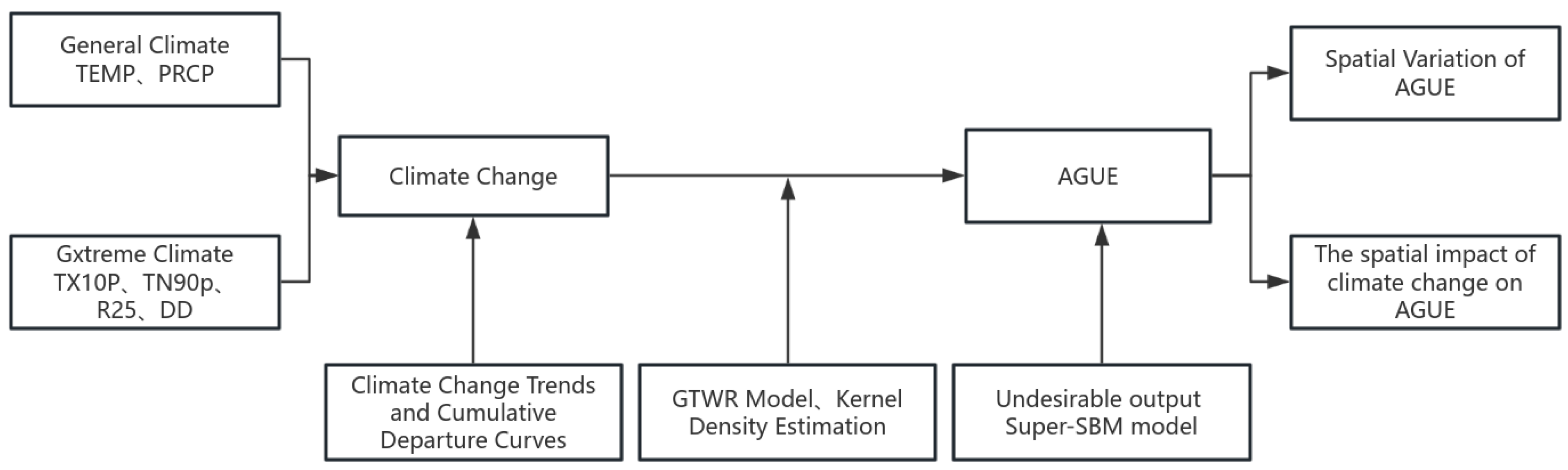
2.4. Research Process

Based on the preset research methods and data system, this study conducts a systematic analysis of the impact mechanism of climate change on the green utilization efficiency of agricultural land. The specific research process is shown in the process diagram (Figure 1).

3. Results and Analysis

3.1. Spatiotemporal Characteristics of Climate Change Nationwide

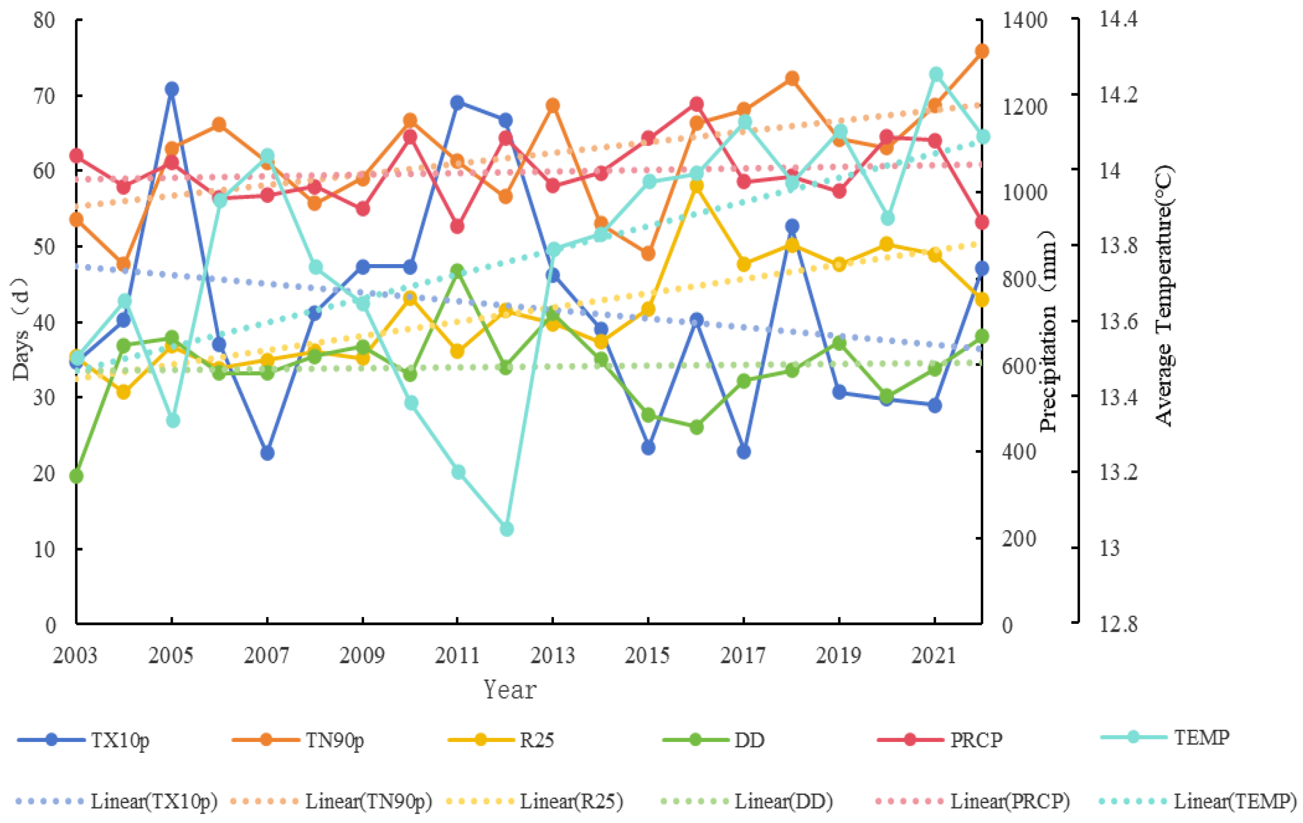
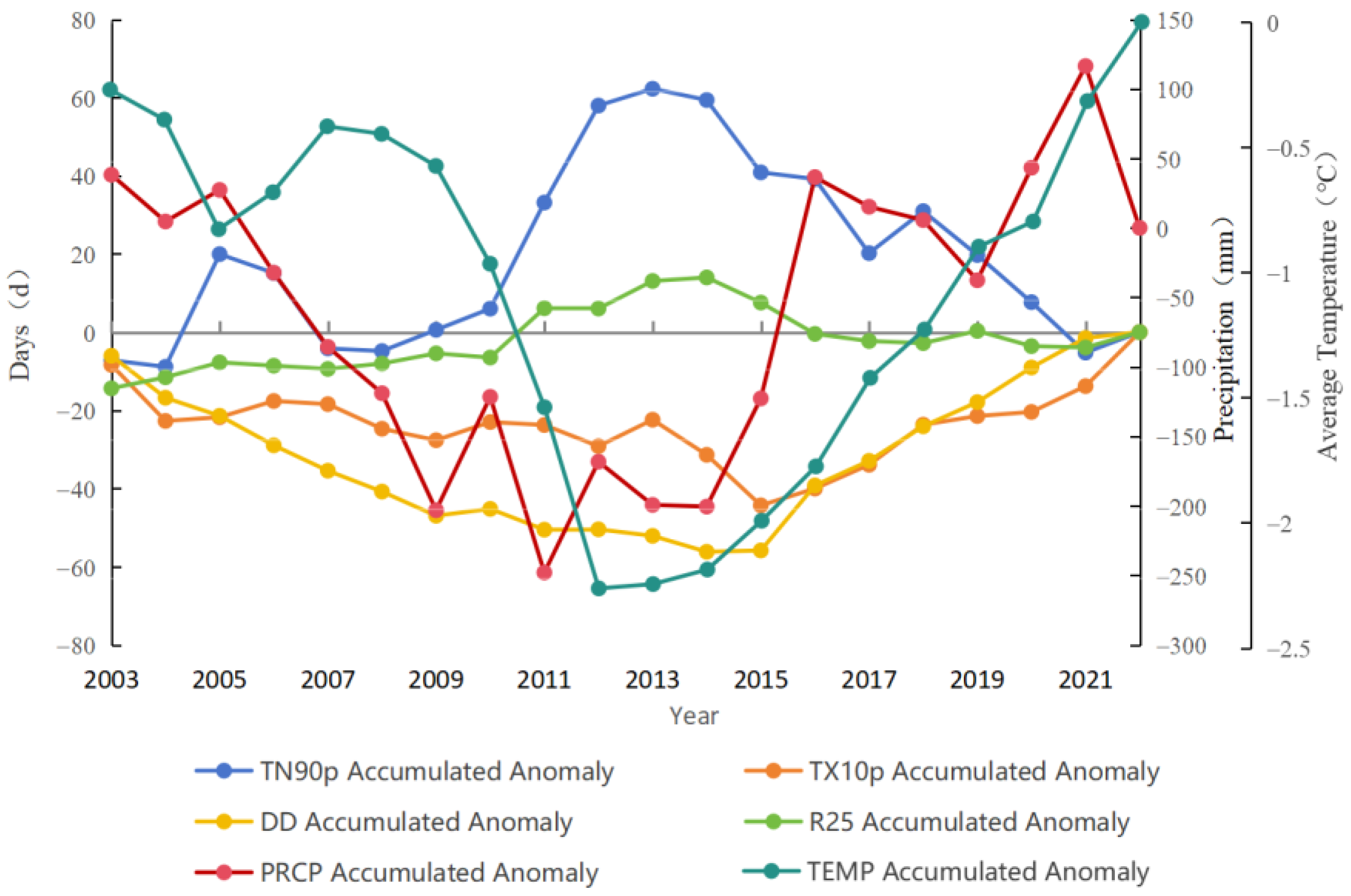
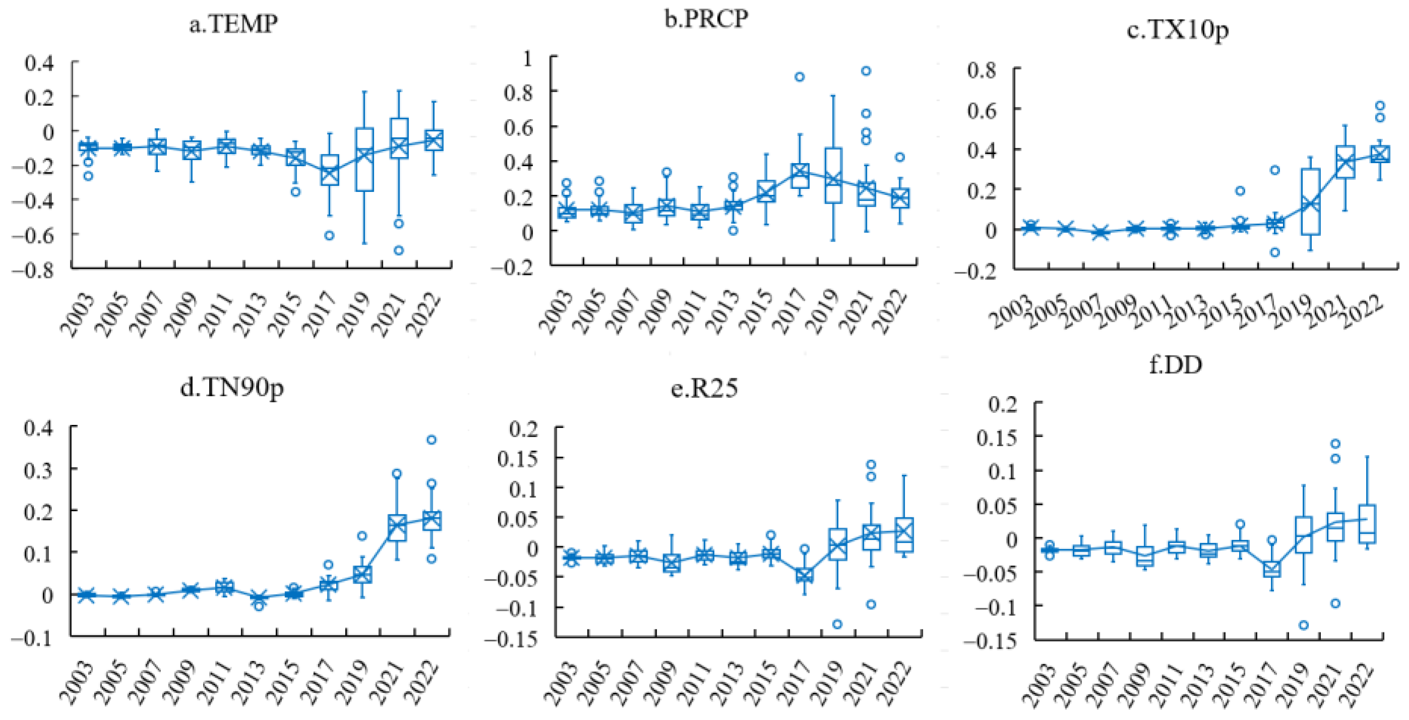
3.1.1. Temporal Characteristics of Annual Climate Change

As shown in Figure 2, the average annual temperature from 2003 to 2022 was 13.77 °C. The average temperature trend rate was 0.32 °C/10a. The highest annual average temperature occurred in 2021 at 14.25 °C, while the lowest was recorded in 2012 at 13.05 °C. The difference between these extremes is 1.2 °C. As shown in Figure 3, the cumulative departure curve of annual average temperature can be divided into four stages. From 2003 to 2005, the curve shows a downward trend, indicating that the temperature during this period was generally lower than the long-term average. Since 2005, the curve began to show an upward trend, suggesting that the temperature began to rise. This upward trend continued until 2007 when the curve started to decline, and the downward trend persisted until 2012. After 2012, the temperature has generally been higher than the long-term average, with the annual average temperature continuously increasing, and the cumulative departure curve showing an upward trend. Therefore, it is evident that the trend of climate warming in China is significant.

The long-term average annual precipitation in China is 1046.80 mm. During the study period, the lowest annual precipitation was recorded in 2011 at 920.45 mm, while the highest was in 2016, reaching 1206.03 mm. The difference between the highest and lowest precipitation amounts to 285.58 mm, indicating some fluctuation in annual precipitation. From 2003 to 2022, the climate trend rate of precipitation in China was 18.81 mm/10a, showing an increasing trend. Throughout the study period, the cumulative level of precipitation fluctuated up and down, with the amplitude of fluctuation gradually increasing.

3.1.2. Temporal Characteristics of Extreme Climate Change

Analyzing the data from Figure 2, the study period shows a tendency rate of extreme low temperatures decreasing by 5.75% per decade. The overall trend of the extreme-low-temperature curve is downward, indicating a reduction in both the probability and intensity of low-temperature weather occurrences each year. On the other hand, the extreme-high-temperature tendency rate shows an increase of 7.05% per decade, exhibiting an overall upward trend. This suggests that the probability and intensity of high-temperature weather are gradually increasing annually. These changing trends are consistent with the overall trend of global warming and rising temperatures. The interannual variation in extreme rainfall in China was relatively stable from 2003 to 2015. However, in 2016, there was a noticeable peak, reaching 58.05 d. After 2016, the number of extreme rainfall days decreased but remained higher than the period from 2003 to 2015. The number of drought days in China has been relatively stable, with a multi-year average of 34.11 d. In the study period, 2003 marked the lowest peak with a value of 19.72 days.

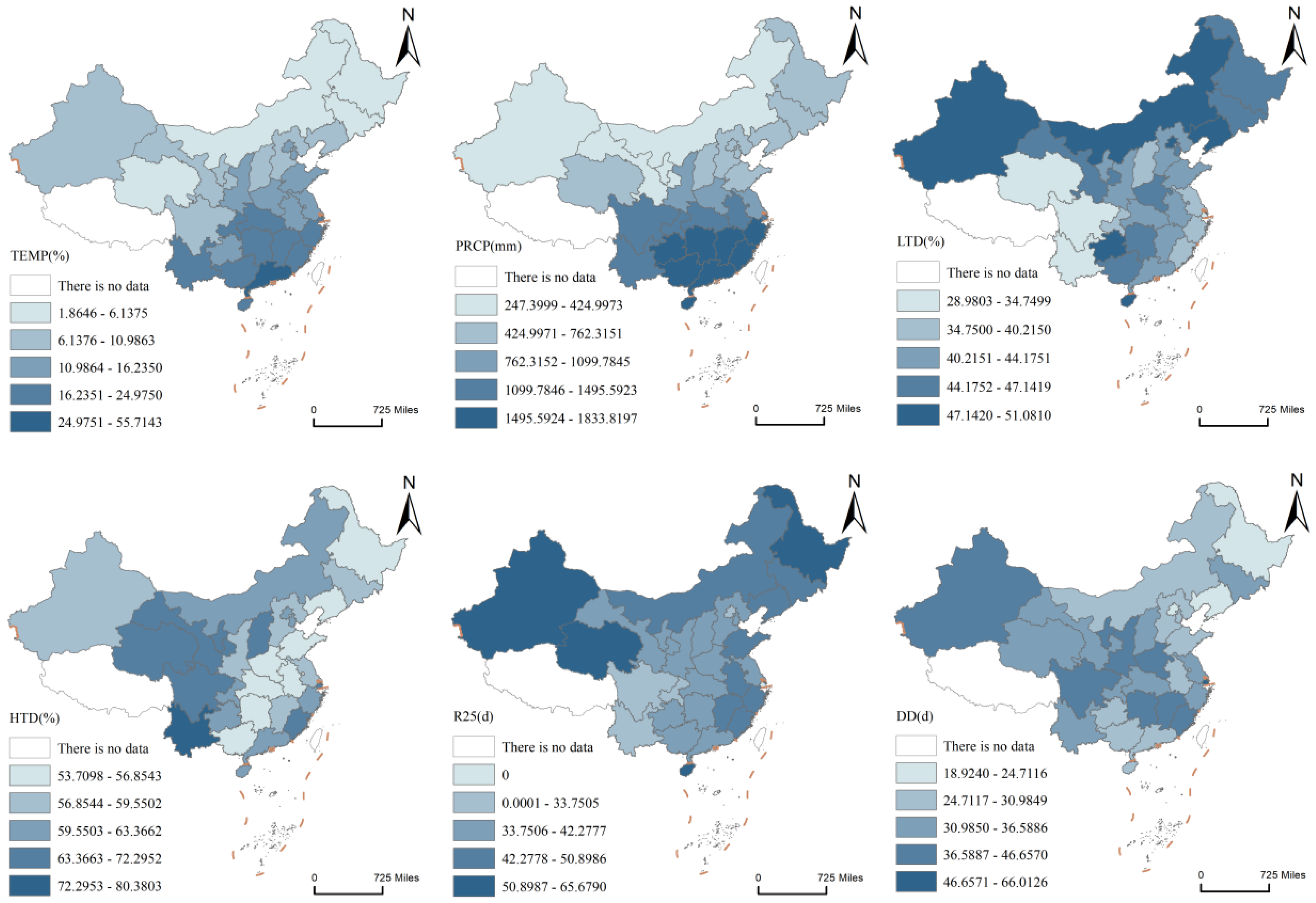
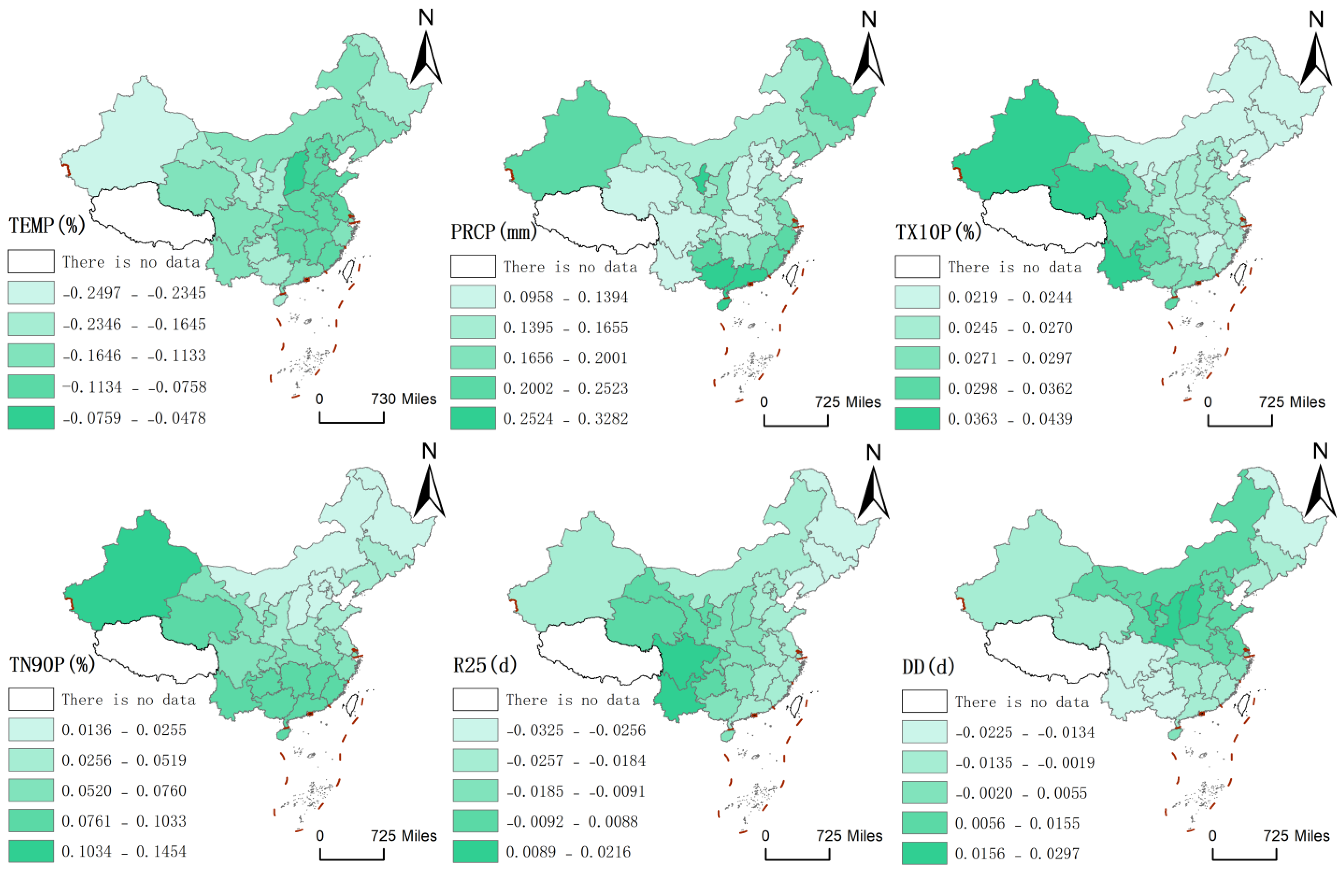
3.1.3. Spatial Characteristics of Climate Change

As shown in Figure 4, in this study, with the spatial analysis function of ArcGIS 10.8 software, the natural break point classification method was used to process and analyze various climate data. Overall, general climate change generally exhibits a significant spatial distribution feature of “higher in the south and lower in the north”. This aligns with the latitudinal differentiation of China’s climatic zones, which range from south to north. Extreme low temperatures show a decreasing trend from south to north, while extreme high temperatures are predominantly concentrated in the southeastern regions. Extreme precipitation mainly occurs in the northwest and northeast parts of the country. The number of drought days tends to decrease from the interior to the exterior. Notably, the Xinjiang region experiences both higher extreme precipitation and extreme drought, possibly due to the combined effects of its geographical location, topography, and climatic features. Specifically, this may be attributed to Xinjiang’s pronounced continental characteristics, its span from mid-latitudes to some high latitudes, and the polar amplification effects in high-latitude areas.

3.2. Results of AGUE Measurement

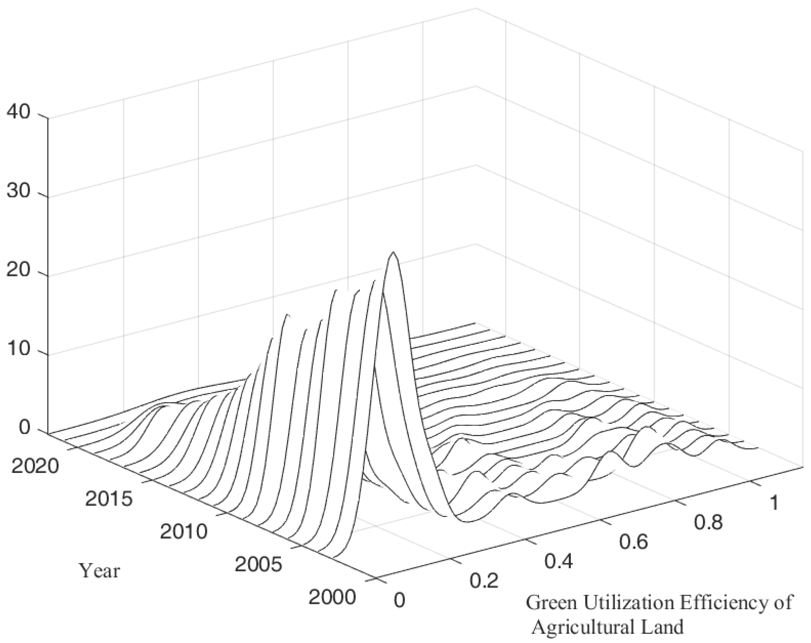
3.2.1. Temporal Variation Characteristics of AGUE

This study used kernel density estimation to analyze the dynamic trends of AGUE in various regions from 2003 to 2022. Figure 5 illustrates that the AGUE kernel density curve has shifted to the left over time, indicating a general decline in AGUE across most regions. From the perspective of the main peak’s shape, the height of the main peak in the kernel density curve shows a fluctuating decline. Meanwhile, it exhibits a trend of shifting from a broad peak to a narrow peak. This suggests that during the study period, the dispersion of AGUE has changed from a divergent state to a convergent state. The efficiency gap among different regions is gradually narrowing, indicating a tendency towards concentration. In terms of the distributional ductility of the kernel curve, the curve exhibited a right-skewed tail to a certain extent in the early stage of the study. This indicates that in the early period, the AGUE in some regions across the country was significantly higher than that in other regions. After 2015, the right-skewed tail phenomenon almost vanished, suggesting that the nationwide AGUE is approaching an average level.

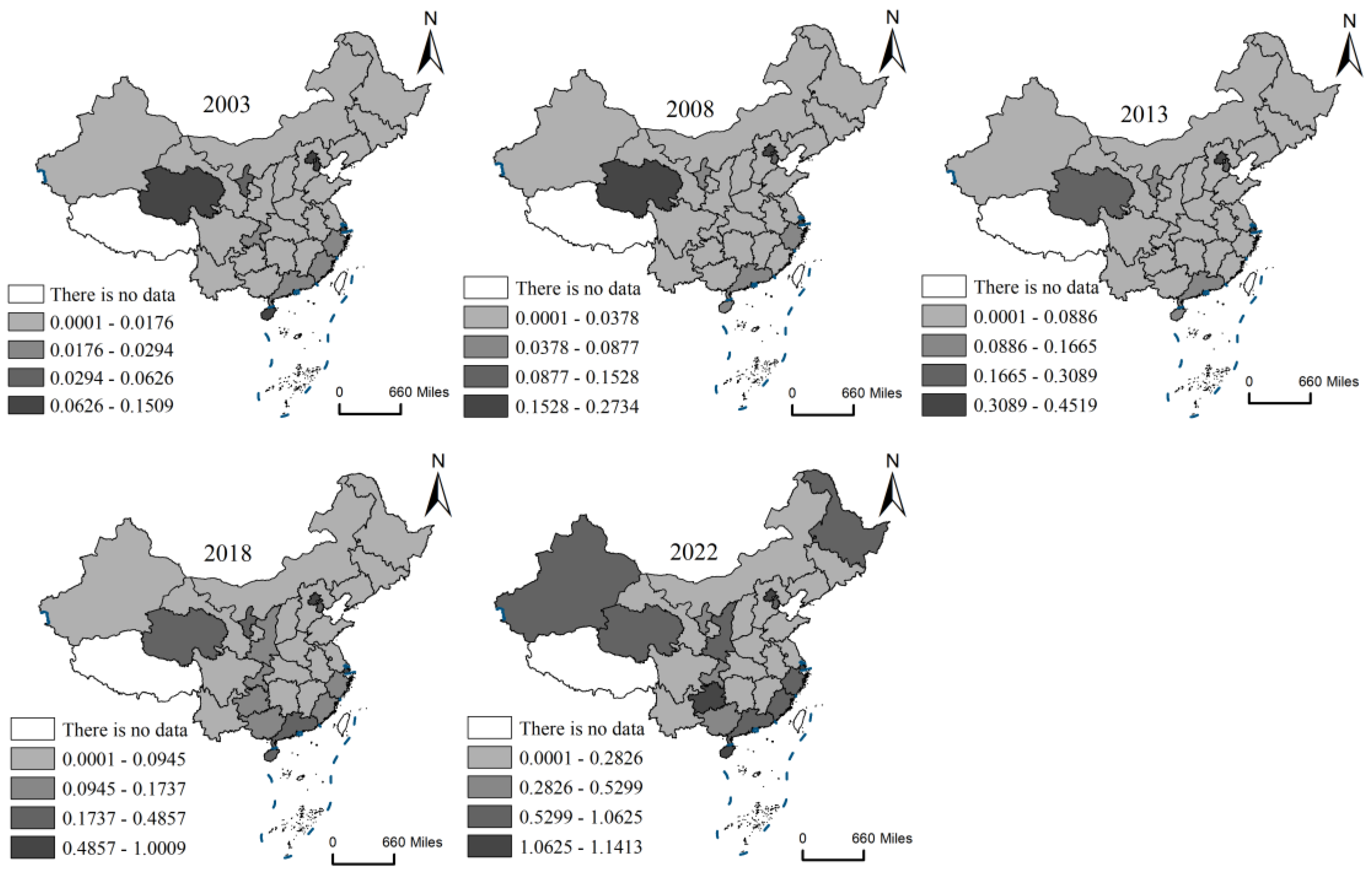
3.2.2. Spatial Variation of AGUE

In this study, with the spatial analysis function of ArcGIS 10.8 software, the natural break point classification method was used to process and analyze various climate data. As shown in Figure 6, the spatial distribution of AGUE nationwide shows an intertwined pattern of high and low efficiency, with some regions exhibiting a tendency towards concentration. Overall, there are significant regional disparities. The AGUE nationwide demonstrates a “W”-shaped fluctuating growth trend. Looking at the multi-year average values, Beijing has the highest AGUE value of 0.50, while Shandong has the lowest, at only 0.02. During the study period, Heilongjiang experienced the largest increase in efficiency, reaching 84.03%, whereas Inner Mongolia had the slowest growth, at just 3.41%. The AGUE in all 30 regions covered by the study data showed an increase. Therefore, in most regions across the country, there is still substantial room for improvement in AGUE.

3.3. GTWR Model Validation

3.3.1. Test of Spatiotemporal Non-Stationarity

As shown in

Table 2. Comparison of model parameters.

Evaluation Index	OLS	TWR	GWR	GTWR
R2	0.520	0.527	0.523	0.670
Adjusted R 2	0.507	0.518	0.514	0.664
AICc	−560.014	−563.695	−559.373	−692.337
Bandwidth	—	1.987	1.988	0.165
Residual Squares	—	13.098	13.195	9.129
Sigma	—	0.148	0.148	0.123

, to examine the applicability of the GTWR model, that is, to detect whether the sample exhibits significant temporal and spatial non-stationarity, this study first employs a global Ordinary Least Squares (OLS) regression to analyze the impact of climate change on the green utilization efficiency of agricultural land without considering any temporal or spatial factors. Subsequently, Temporally Weighted Regression (TWR), Geographically Weighted Regression (GWR), and Geographically and Temporally Weighted Regression (GTWR) models are constructed from the perspectives of time, space, and a combined spatiotemporal approach, respectively, for comparative analysis. The study selects the coefficient of determination (R²), the corrected Akaike Information Criterion (AICc), the Residual Squares, and the square root of the normalized residual sum of squares (Sigma) as evaluation metrics. Among them, the value of R² ranges from 0 to 1, with a higher value indicating a stronger explanatory power of the model. The AICc value is used to assess model performance, with a lower value suggesting a better fit between the model and the observed data. Similarly, lower values of Residual Squares and Sigma indicate a superior fitting effect of the model.

Table 2 presents a comparison of the parameters among the OLS model, the TWR model, the GWR model, and the GTWR model. Among these, the GTWR model has the highest R² value of 0.670, indicating that it possesses the greatest explanatory power compared to the other models. Its AICc value is −692.377, which is significantly better than those of the other models. Additionally, the GTWR model exhibits the lowest values for both the Residual Squares and Sigma metrics. Based on a comprehensive comparison of these parameters, it can be concluded that the GTWR model is more suitable for explaining the impact of climate change on the green utilization efficiency of agricultural land.

3.3.2. Spatial Autocorrelation

The data in

Table 3. Global Moran’s I results for AGUE.

Year	Moran’s I	Z-Value	p-Value	Year	Moran’s I	Z-Value	p-Value
2003	0.188	2.720	0.007	2013	0.099	1.607	0.108
2004	0.132	2.170	0.030	2014	0.213	3.164	0.002
2005	0.216	3.135	0.002	2015	0.212	3.101	0.002
2006	0.201	3.334	0.000	2016	0.152	2.623	0.009
2007	0.131	2.315	0.021	2017	0.175	2.631	0.009
2008	0.207	3.097	0.002	2018	0.204	3.075	0.002
2009	0.136	2.187	0.029	2019	0.190	2.818	0.005
2010	0.013	0.543	0.587	2020	−0.059	−0.36	0.719
2011	0.129	2.001	0.045	2021	0.260	3.665	0.000
2012	0.198	2.919	0.004	2022	0.228	3.328	0.000

reveal that the Global Moran’s I, which measures the spatial autocorrelation of AGUE at the inter-provincial level in China from 2003 to 2022, is predominantly significant at the 1% level. This indicates a notable positive spatial autocorrelation in nationwide AGUE during the study period, with pronounced clustering, thereby supporting the applicability of the GTWR model. Within the study period, Moran’s I fluctuates significantly between 0.260 and 0.013, with an average of 0.161, demonstrating considerable annual variability. The overall trend exhibits a fluctuating increase in Moran’s I, indicating an intensification of spatial clustering in AGUE and a widening of regional disparities, revealing an imbalance in the spatial distribution pattern.

3.4. GTWR Model Regression Results

3.4.1. Analysis of the Temporal Evolution of Climate Change

In this study, with the spatial analysis function of ArcGIS 10.8 software, the natural break point classification method was used to process and analyze various climate data. The blue crosses and circles in Figure 7 represent mean and outliers of the data, respectively. Figure 7a illustrates that the regression coefficients of average temperature from 2003 to 2022 are all less than 0, with a mean of −0.130. Considering the overall trend of rising average temperature nationwide, this indicates that the increase in temperature has a negative impact on AGUE. While higher temperatures can boost crop yields to some extent, excessively high temperatures enhance water requirements for crops, leading to increased demand for agricultural irrigation and decreased water use efficiency, thus lowering the overall AGUE. Figure 7b reveals that the regression coefficients of annual precipitation are predominantly positive during the study period, with a multi-year average of 0.186. Given the limited water resources nationwide and the imbalance of water resources among regions, the increase in annual precipitation can effectively alleviate water scarcity in some areas, thereby enhancing agricultural productivity and exerting a positive impact on the improvement of AGUE. Overall, in the context of general climate assumptions, the increase in annual average temperature has a negative effect on AGUE, whereas the increase in annual precipitation has a positive effect. Consequently, hypotheses H1a and H1b are both supported.

During the study period from 2003 to 2022, the regression coefficients of extreme cold and extreme heat events both exhibit a shift from negative to positive trends in China (Figure 7c–d). One possible reason is that in the early stages following the occurrence of extremely low and high temperatures, they may have a negative impact on AGUE. Over time, AGUE has improved in adapting to extreme temperature conditions, which could be related to the implementation of agricultural technology and management practices. However, the dispersion of extreme heat and extreme cold events has increased, indicating a gradual rise in the frequency and intensity of these events, accompanied by a certain degree of uncertainty. Figure 7e shows that the mean regression coefficient of extreme precipitation is −0.013, with minor fluctuations and negative values in the early stages. A significant fluctuation occurred in 2017, when 43 large-scale heavy rainfall events were recorded nationwide, predominantly during the main flood season. Figure 7f indicates that the regression coefficient of drought days fluctuates around 0 throughout the study period. The increased dispersion underscores the need to pay more attention to the impact of drought days on AGUE. The findings deviate from expectations, as extreme weather initially tends to suppress AGUE. However, continuous exposure to extreme weather forces farming entities to adapt, leading to increased investments in capital, technology, and infrastructure for farmland utilization. Consequently, in the later stages of the study, extreme weather conditions appear to enhance AGUE.

3.4.2. Spatial Variation Characteristics of Climate Change

The regression coefficients of TEMP in Figure 8 are negative, exhibiting a spatial distribution pattern that gradually weakens from southeast to northwest. Conversely, the regression coefficients of PRCP are positive, showing a spatial distribution characteristic that decreases from the periphery to the center. The possible reasons for the above-mentioned spatial differences in general climate firstly lie in the spatial distribution characteristics of climatic elements and the spatial distribution patterns of climate change among different provinces. These factors collectively contribute to the distinct climatic characteristics and variations observed in different regions. The spatial distribution of the regression coefficients for average temperature is roughly analogous to the pattern of average temperature itself but contrasts with the spatial pattern of temperature trends. In regions with higher average temperatures, crops that thrive in warmth are typically grown, and efficient irrigation methods are employed, enhancing AGUE.

Secondly, AGUE correlates with climate factors. Regions like Hainan, Guangdong, and Qinghai consistently exhibit high AGUE levels during the study period, with smaller impact coefficients from annual average temperature. In contrast, in regions with lower AGUE, such as Henan and Anhui, the influence of annual average temperature is more pronounced. Simultaneously, the spatial distribution of annual precipitation shows similarities with AGUE, particularly in central regions where AGUE is relatively lower and the impact of precipitation is diminished. Additionally, China’s vast territory encompasses diverse landscapes, including coastal areas, hills, and the basins of the Yellow River and the Yangtze River. In these varied geographical settings, temperature often negatively affects AGUE. Particularly in coastal regions, the impact of precipitation on AGUE is more pronounced.

From an extreme climate perspective, regions with high extreme-low-temperature coefficients are mainly distributed in Xinjiang and Qinghai. Areas with high extreme-high-temperature coefficients are primarily located in Xinjiang, Qinghai, Sichuan, Chongqing, and Yunnan. Positive drought day coefficients are mainly found in Yunnan, Sichuan, and Chongqing. Positive extreme rainfall coefficients are mainly distributed in Shanxi, Shaanxi, Henan, Anhui, Jiangsu, Shandong, Hebei, Inner Mongolia, and Ningxia. Due to various factors such as geographical environment, climatic conditions, and economic development levels, provinces differ in their sensitivity to and resilience against extreme climate events. Some regions may be more vulnerable to extreme climate effects, while others exhibit greater resilience. It is important to note that extreme climate events often do not occur in isolation. For example, Yunnan, Sichuan, and Chongqing may face multiple extreme climate events simultaneously, such as the “high-temperature drought”, a compound extreme climate event. Central regions need to pay attention to the impacts of extreme rainfall weather.

4. Discussion

4.1. Interannual Variability and Spatial Heterogeneity of Climate Risk

The rising trend of China’s annual mean temperature, coupled with the spatial pattern of “higher in the south and lower in the north”, exacerbates regional imbalances in agricultural production. In the eastern and southern regions, increased heat resources may lead to intensified pest and disease pressures and shortened crop growth periods. Conversely, while warming in the western and northern regions could potentially extend the growing season, the issue of water scarcity will become even more pronounced. China’s annual precipitation remains generally stable, yet significant spatial variations exist. This precipitation pattern necessitates differentiated climate change adaptation strategies across regions. For instance, the North China Plain, with relatively low precipitation, focuses on efficient water use and drought resistance. In contrast, the Jiangnan region, with abundant rainfall, must address flood prevention and rational water resource allocation. Given these circumstances, homogenized climate services are insufficient for diverse regional needs. Hence, constructing a hierarchical and multi-scale monitoring and early-warning system is crucial. Utilizing meteorological satellites and ground observation networks, a comprehensive climate monitoring cloud platform covering the entire cycle should be established, enabling real-time sharing of conventional indicators such as temperature and precipitation. For extreme climate events, the “impact chain” early-warning model from Europe and the United States can be referenced, decomposing the disaster process into three stages, “threshold breach, duration, and spatial extent”, for dynamic assessment. Among them, threshold breach refers to setting critical thresholds for climate elements based on historical climate data bits, and conducting dynamic monitoring and real-time early warning. Duration refers to the assessment of the duration of extreme climate events and the determination of their potential impacts on ecosystems and human society. The spatial extent refers to determining the impact range of extreme climate events and assessing the vulnerability and exposure of the affected areas. By dynamically evaluating the three stages of the “impact chain”, the development trend of extreme climate events can be predicted more accurately, providing a scientific basis for disaster response.

4.2. Dynamic Evolution of AGUE

The disappearance of leftward shift in the kernel density curve and the rightward long tail indicates that the AGUE is showing a downward trend, and the efficiency gap between regions is narrowing. This may be attributed to the aggravation of agricultural non-point source pollution and over-exploitation of cultivated land. Therefore, caution is advised against regional development imbalances resulting from the “club convergence” of efficiency. It is suggested to implement an efficiency decline early-warning mechanism and initiate special inspections for regions where AGUE has continuously declined for three years, with a focus on checking excessive use of chemical fertilizers and pesticides and residual film issues. Simultaneously, an efficiency improvement incentive fund should be established to provide policy preferences for regions with significant efficiency improvements.

4.3. The Impact of Annual Climate Change on AGUE

The study reveals that annual rainfall significantly boosts AGUE, whereas average temperature has a detrimental effect. As a core natural factor in agricultural production, annual precipitation directly alleviates water stress in arid regions by its increase, providing essential moisture conditions for crop growth. In arid and semi-arid regions, increased rainfall significantly enhances soil moisture, extends the crop growth period, and promotes photosynthesis and nutrient uptake, thereby increasing yield per unit area. While precipitation generally exerts a beneficial impact, its uneven spatial and temporal distribution can potentially give rise to flooding. Therefore, it is necessary to optimize cropping systems in conjunction with precipitation forecasting models, such as promoting flood-tolerant varieties or adjusting sowing dates to avoid peak rainy seasons. Additionally, constructing field drainage systems and rainwater collection facilities can further enhance the efficiency of precipitation use, maximizing the marginal benefits of natural rainfall. In terms of temperature effects, rising temperatures suppress AGUE by shortening crop growth periods and reducing photosynthetic efficiency. The increase in temperature leads to a rapid proliferation of pests, resulting in a surge in pesticide use, which in turn reduces the AGUE. In the future, efforts should be accelerated to cultivate heat-tolerant varieties, such as improving the heat tolerance of rice through gene editing techniques, and promoting agronomic practices like intercropping and cover cropping to mitigate the adverse effects of rising surface temperatures on crops.

4.4. The Impact of Extreme Climate Change on AGUE

The influence of extreme climate change on AGUE is characterized by its multidimensionality, regional variability, and long-term nature. It not only directly damages agricultural production but also indirectly reduces system sustainability through resource constraints and ecological degradation. Future strategies should shift from “passive defense” to “active adaptation,” constructing a multi-tiered climate resilience system through technological innovation, institutional optimization, and regional collaboration. Integrating climate adaptation with green transformation is essential for achieving a win–win scenario of high-quality agricultural development and ecological security.

Current research has several limitations. First, while it analyzes the impact of climate change on AGUE, it does not explore the underlying mechanisms due to model and data constraints. Second, the measurement of AGUE primarily relies on provincial panel data from statistical yearbooks, lacking support from plot-level operational data of agricultural entities. This may obscure the heterogeneity of microentities in efficiency assessments. Future research is recommended to incorporate farmer survey data and agricultural enterprise operation data to establish a multi-tiered analysis framework.

5. Conclusions

This study reveals the impact of climate change on AGUE, including its spatial and temporal heterogeneity. Firstly, general climate events exhibit significant interannual variability and spatial heterogeneity. The annual average temperature and rainfall show a fluctuating upward trend, and both present a spatial pattern of “higher in the south and lower in the north”. Secondly, AUGE shows a downward trend and exhibits obvious spatial clustering characteristics. Thirdly, the impact of annual climate on AGUE exhibits spatiotemporal heterogeneity. Overall, the average temperature has a significant negative impact and the regression coefficient decreases from southeast to northwest, while the annual precipitation has a significant positive impact and the regression coefficient decreases from the periphery to the center. Fourthly, extreme weather significantly reduced AGUE and exhibited regional imbalances.

References

1. Li, T.; Sun, X.; Feng, K. The Design of Food Security System Based on Feasible Ability Theory in China: Labor Transfer, Logic of Factor Substitution and Feasible Ability Improvement. Econ. Probl. 2020, 9, 100–108. [Google Scholar]
2. Rezaei, E.E.; Webber, H.; Asseng, S.; Boote, E.; Durand, J.L.; Ewert, F.; Martre, P.; MacCarthy, D.S. Climate change impacts on crop yields. Nat. Rev. Earth Environ. 2023, 4, 831–846. [Google Scholar] [CrossRef]
3. Zhu, J.; Wang, M.; Zhang, C. Impact of high-standard basic farmland construction policies on agricultural eco-efficiency: Case of China. Natl. Account. Rev. 2022, 4, 147–166. [Google Scholar] [CrossRef]
4. Ye, F.; Wang, L.; Razzaq, A.; Tong, T.; Zhang, Q.; Abbas, A. Policy impacts of high-standard farmland construction on agricultural sustainability: Total factor productivity-based analysis. Land 2023, 12, 283. [Google Scholar] [CrossRef]
5. Liu, Y.; Liu, Y.; Guo, L. Impact of climatic change on agricultural production and response strategies in China. Chin. J. Eco-Agric. 2010, 18, 905–910. [Google Scholar] [CrossRef]
6. Wu, S.; Zhao, D. Progress on the impact, risk and adaptation of climate change in China. China Popul. Resour. Environ. 2020, 30, 1–9. [Google Scholar]
7. Jin, W.; Jin, S. Accelerating China’s Transformation into an Agricultural Powerhouse:Present Basis, International Experiences and Path Selection. Chin. Rural. Econ. 2023, 01, 18–32. [Google Scholar]
8. Ozdemir, D. The impact of climate change on agricultural productivity in Asian countries: A heterogeneous panel data approach. Environ. Sci. Pollut. Res. 2022, 29, 8205–8217. [Google Scholar] [CrossRef]
9. Chou, J.; Dong, W.; Hong, J.; Tu, G. New Ideas for Research on the Impact of Climate Change on China’s Food Security. Clim. Environ. Res. 2022, 27, 206–216. [Google Scholar]
10. He, L.; Mao, L. Change of soybean climatic suitability in Northeast China under climate change. Chin. J. Eco-Agric. 2023, 31, 690–698. [Google Scholar]
11. Dai, M.; Yu, W. Research on Enhancing Agricultural Green Development Capability Under the Background of Climate Change. Acad. J. Zhongzhou 2024, 4, 49–56. [Google Scholar]
12. Enete, I.C. Impacts of climate change on agricultural production in Enugu State, Nigeria. J. Earth Sci. Clim. Change 2014, 5, 234. [Google Scholar]
13. Habib-ur-Rahman, M.; Ahmad, A.; Raza, A.; Hasnain, M.U.; Alharby, H.F.; Alazhrani, Y.M.; Bamagoos, A.A.; Hakeem, K.R.; Ahmad, S.; Nasim, W. Impact of climate change on agricultural production; Issues, challenges, and opportunities in Asia. Front. Plant Sci. 2022, 13, 925548. [Google Scholar] [CrossRef]
14. Lv, T.; Fu, S.; Hu, H.; Wang, L.; Geng, C. Dynamic Evolution and Convergence Characteristics of Cultivated Land Green Use Efficiency Based on the Constraint of Agricultural Green Transition: Taking the Main Grain Producing Areas in the Middle Reaches of the Yangtze River as an Example. China Land Sci. 2023, 37, 107–118. [Google Scholar]
15. Li, Y.; Chen, Y. Development of an SBM-ML model for the measurement of green total factor productivity: The case of pearl river delta urban agglomeration. Renew. Sustain. Energy Rev. 2021, 145, 111131. [Google Scholar] [CrossRef]
16. Chen, Y.; Miao, J.; Zhu, Z. Measuring green total factor productivity of China’s agricultural sector: A three-stage SBM-DEA model with non-point source pollution and CO2 emissions. J. Clean. Prod. 2021, 318, 128543. [Google Scholar] [CrossRef]
17. Yu, J.; Zhou, K.; Yang, S. Land use efficiency and influencing factors of urban agglomerations in China. Land Use Policy 2019, 88, 104143. [Google Scholar] [CrossRef]
18. Zhao, Q.; Bao, H.X.H.; Zhang, Z. Off-farm employment and agricultural land use efficiency in China. Land Use Policy 2021, 101, 105097. [Google Scholar] [CrossRef]
19. Wu, W.; Verburg, P.H.; Tang, H. Climate change and the food production system: Impacts and adaptation in China. Reg. Environ. Change 2014, 14, 1–5. [Google Scholar] [CrossRef]
20. Lee, C.; Zeng, M.; Luo, K. How does climate change affect food security? Evidence from China. Environ. Impact Assess. Rev. 2024, 104, 107324. [Google Scholar] [CrossRef]
21. Zheng, S.; Liu, J.; An, N. The impact of natural risks on the allocation efficiency of farmland resources: From the perspective of risk coping capability differences. Resour. Sci. 2024, 46, 829–840. [Google Scholar]
22. He, J.; Yang, J. Spatial—temporal characteristics and influencing factors of land-use carbon emissions: An empirical analysis based on the GTWR model. Land 2023, 12, 1506. [Google Scholar] [CrossRef]
23. Jin, S.; Zhang, Z.; Hu, Y.; Du, Z. Historical Logic, Theoretical Interpretation, and Practical Exploration of China’s Agricultural Green Transformation. Issues Agric. Econ. 2024, 3, 4–19. [Google Scholar]
24. Ren, J.; Zhang, M.; You, S. Study on the Impact of Natural Disasters on Agricultural Production and Macroeconomy in China. Sci. Decis. Mak. 2024, 8, 55–79. [Google Scholar]
25. Luo, W.; Hu, X.; Sun, H. Study on Influence of Environment Degradation Perception and Family Endowment on Farmers’ Well-Being in Arid Areas—Based on an Empirical Analysis of 1317 Survey Data from Gansu Province. For. Econ. 2022, 44, 42–59. [Google Scholar]
26. Yin, S.; Yang, X.; Chen, J. Adaptive behavior of farmers’ livelihoods in the context of human-environment system changes. Habitat Int. 2020, 100, 102185. [Google Scholar] [CrossRef]
27. Chen, S.; Huang, Y. Effect of Climate Change on Fertilizer Use Efficiency of Double-Season Rice:A Case Study of Southern Rice Growing Region. J. Agro-For. Econ. Manag. 2023, 22, 582–591. [Google Scholar]
28. Chou, H.; Huang, Q. The Green Transformation of Agriculture and High-quality Development:Theoretical Logic and Practice. Issues Agric. Econ. 2025, 2, 15–23. [Google Scholar]
29. Erbas, C.; Solakoglu, G. In the presence of climate change, the use of fertilizers and the effect of income on agricultural emissions. Sustainability 2017, 9, 1989. [Google Scholar] [CrossRef]
30. Olesen, J.E.; Bindi, M. Consequences of climate change for European agricultural productivity, land use and policy. Eur. J. Agron. 2002, 16, 239–262. [Google Scholar] [CrossRef]
31. Meite, F.; Alvarez-Zaldívar, P.; Crochet, A.; Wiegert, C.; Payraudeau, S.; Imfeld, G. Impact of rainfall patterns and frequency on the export of pesticides and heavy-metals from agricultural soil. Sci. Total Environ. 2018, 616, 500–509. [Google Scholar] [CrossRef] [PubMed]
32. Zhou, S.; Zhou, W.; Zhu, H.; Wang, C.; Wang, Y. Impact of Climate Change on Agriculture and its Countermeasures. J. Nanjing Agric. Univ. 2010, 10, 34–39. [Google Scholar]
33. Chen, Y.; Zeng, M.; Chen, B. Impact of climate change on the resilience of food production: Research of the moderating effect based on crop diversification. Acta Ecol. Sin. 2024, 44, 6937–6951. [Google Scholar]
34. Zhang, H. Impact of Climate Change on Ecosystems and Agricultural Production. J. Agric. Catastrophology 2023, 13, 201–203. [Google Scholar]
35. Wang, Y.; Chen, W. Extreme Climate, Agricultural Machinery Operation Service Market and Food Production:An Empirical Analysis Based on Panel Data from 13 Major Grain-producing Areas. J. Agrotech. Econ. 2024, 10, 70–90. [Google Scholar]
36. Yi, Z.; Liu, W. Variations of the Extreme Temperature in Wushui River Basin during the past 57 Years. China Rural. Water Hydropower 2018, 12, 106–109. [Google Scholar]
37. Mudelsee, M. Trend analysis of climate time series: A review of methods. Earth-Sci. Rev. 2019, 190, 310–322. [Google Scholar] [CrossRef]
38. Tone, K. A slacks-based measure of super-efficiency in data envelopment analysis. Eur. J. Oper. Res. 2002, 143, 32–41. [Google Scholar] [CrossRef]
39. Li, H.; Fang, K.; Yang, W.; Wang, D.; Hong, X. Regional environmental efficiency evaluation in China: Analysis based on the Super-SBM model with undesirable outputs. Math. Comput. Model. 2013, 58, 1018–1031. [Google Scholar] [CrossRef]
40. Fotheringham, A.S.; Crespo, R.; Yao, J. Geographical and temporal weighted regression (GTWR). Geogr. Anal. 2015, 47, 431–452. [Google Scholar] [CrossRef]
41. Song, M.; Wu, Q.; Zhu, H. Could the aging of the rural population boost green agricultural total factor productivity? Evidence from China. Sustainability 2024, 16, 6117. [Google Scholar] [CrossRef]
42. Climate Change 2013. The Physicle Science Basis Technical Summary. IPCC. 2013. Available online: https://www.ipcc.ch/report/ar5/wg1/ (accessed on 13 October 2024).
43. Wu, F.; Li, L.; Zhang, H.; Chen, H. Net Carbon Emissions of Farmland Ecosystem Influenced by Conservation Tillage. J. Ecol. 2007, 26, 2035–2039. [Google Scholar]
44. Dubey, A.; Lal, R. Carbon Footprint and Sustainability of Agricultural Production Systems in Punjab, India and Ohio, USA. Croplmprovement 2009, 23, 332–350. [Google Scholar] [CrossRef]
45. Hong, H.; Li, F.W.; Xu, J. Climate risks and market efficiency. J. Econom. 2019, 208, 265–281. [Google Scholar] [CrossRef]
46. Chen, S.; Chen, X.; Xu, J. Impacts of climate change on agriculture: Evidence from China. J. Environ. Econ. Manag. 2016, 76, 105–124. [Google Scholar] [CrossRef]
Figure 1. The study flowchart.
Land 14 01260 g001
Figure 2. Climate change trends, 2003–2022.
Land 14 01260 g002
Figure 3. Cumulative departure curves, 2003–2022.
Land 14 01260 g003
Figure 4. Spatial distribution of national climate indicators’ multi-year averages.
Land 14 01260 g004
Figure 5. Kernel density estimation of AGUE values, 2003–2022.
Land 14 01260 g005
Figure 6. Spatial distribution of AGUE.
Land 14 01260 g006
Figure 7. Trends in climate change regression coefficients, 2003–2022.
Land 14 01260 g007
Figure 8. Spatial variation in the regression coefficients of climate change.
Land 14 01260 g008