Article

Study of Spatial and Temporal Characteristics and Influencing Factors of Net Carbon Emissions in Hubei Province Based on Interpretable Machine Learning

School of Urban Design, Wuhan University, Wuhan 430072, China
*
Author to whom correspondence should be addressed.
Land 2025, 14(6), 1255; https://doi.org/10.3390/land14061255
Submission received: 28 March 2025 / Revised: 20 May 2025 / Accepted: 5 June 2025 / Published: 11 June 2025

Abstract

:
Carbon emissions from global warming pose significant threats to both regional ecology and sustainable development. Understanding the factors affecting emissions is critical to developing effective carbon neutral strategies. This study constructed a precise 1 km resolution net carbon emissions map of Hubei Province, China (2000–2020), and compared the ten distinct machine learning models to identify the most effective model for revealing the relationship between carbon emissions and their influencing factors. The random forest regressor (RFR) demonstrates optimal performance, achieving root mean square error (RMSE) and mean absolute error (MAE) values that are nearly 10 times lower on average than the other models. The results are interpreted using Shapley additive explanation (SHAP), revealing dynamic factor impacts. Our findings include the following. (1) Between 2000 and 2020, net carbon emissions in Hubei increased threefold, with emissions from construction land rising by approximately 7.5 times over the past two decades. Woodland, a major carbon sink, experienced a downward trend. (2) Six key factors are population, the normalized difference vegetation index (NDVI), road density, PM2.5, the degree of urbanization, and the industrial scale, with only the NDVI reducing emissions. (3) Net carbon emissions displayed significant spatial differences and aggregation and are mainly concentrated in the central urban areas of Hubei Province. Overall, this study evaluates various regression models and identifies the primary factors influencing net carbon emissions. The net carbon emission map we have developed can visually identify and locate high-emission hotspots and vulnerable carbon sink areas, thereby providing a direct basis for provincial land use planning.

1. Introduction

Net carbon emissions, also known as net carbon dioxide (CO2) emissions, serve as the primary indicator of greenhouse gas emissions [1]. Understanding net carbon emissions is crucial for solving the problems of global warming and the resulting sustainable development of regional ecosystems and human societies. According to the Fifth Assessment Report (AR5) of the Intergovernmental Panel on Climate Change (IPCC), land use change has emerged as the second largest source of carbon emissions after energy consumption since the pre-industrial era [2]. Land use change contributes approximately 24% to the greenhouse effect [3]. Furthermore, CO2 emissions resulting from land use change constitute one-third of the total CO2 emissions attributed to human activities [4], demonstrating significant spatial variation [5]. Therefore, revealing the characteristics of net carbon emissions from land use and analyzing their relationship with influencing factors will help to formulate differentiated carbon control paths for cities at different stages. The research results could contribute to the development of cities aiming to achieve carbon neutrality by 2060.
Research on net carbon emissions from land use has mainly focused on spatial and temporal characteristics and influencing factors. By analyzing the carbon emission process, such studies identify the key factors affecting land use carbon emissions, so as to provide practical references for reducing carbon emissions. Recent scholars show that the main driving factors affecting net carbon emissions from land use include economic development, land use change, population, and government policy [6,7]. However, variations in research perspectives and scales can influence these relationships [8,9], necessitating tailored analyses of carbon emissions for specific cities when devising carbon neutrality strategies. While traditional models such as the Malmquist model [10], LMDI (logarithmic mean divisia index) decomposition [11], the input–output model [12], STIRPAT (stochastic impacts by regression on population, affluence, and technology) model [13], and the Laspeyres index method [14] have been widely applied to identify driving factors, their linear assumptions may oversimplify complex interactions. Consequently, recent studies have begun integrating machine learning, neural networks, and other advanced algorithms to better elucidate the relationships among these influencing factors. Recent methods, including metaheuristic algorithms such as candle flame optimization (CFO) [15], the perfumer optimization algorithm (POA) [16], makeup artist optimization algorithm (MAOA) [17], revolution optimization algorithm (ROA) [18], and orangutan optimization algorithm (OOA) [19] have shown promise in optimizing complex environmental models by mimicking natural phenomena (e.g., flame dynamics and perfume diffusion). These algorithms are adept at parameter tuning and multi-objective optimization, particularly in scenarios involving high-dimensional and non-convex solution spaces.
In terms of the spatial and temporal characteristics of net carbon emissions from land use change, research has typically been conducted at national or regional levels, with the analysis often segmented by provinces, cities, and counties. At the national level, research has predominantly focused on the provincial scale to elucidate the spatial and temporal distribution patterns of carbon emissions [20]. This includes studies on total carbon emission changes [21], impacts of land use change [22], and emissions from various sectors such as agriculture [23] and transportation [24]. However, studies at the county level remain relatively scarce. Additionally, some national studies have utilized night lighting data to estimate carbon emissions across China, comparing emissions across different administrative units such as provinces, cities, and counties [25]. Nevertheless, the most common carbon emission models still rely on provincial carbon emission data for their analyses, which suggests that there is room to improve estimation accuracy [9,26]. The existing research on Hubei’s carbon emissions predominantly utilizes provincial-level statistical data and conventional linear regression approaches and presents constraints. First, the prevalent reliance on aggregated city/county-level data results in spatial resolution limitations that obscure intra-urban emission patterns and impede the precise identification of fine-scale spatial heterogeneity. Second, conventional linear modeling frameworks demonstrate insufficient capacity to capture complex nonlinear interactions between critical factors, including urbanization processes, vegetation dynamics, and industrial development trajectories. Overall, there is a lack of research on the precise characteristics of net carbon emissions from land use and insufficient exploration of time series variations [27].
Considering the above aspects, high-precision research on the spatial pattern and influencing factors of net carbon emissions from land use change holds significant research value and potential. Such research can improve the feasibility of formulating carbon-neutral plans, which is crucial for determining effective carbon-neutral strategies. The advantages of machine learning models can address the limitations of existing research models in comprehensively and efficiently capturing the influencing factors and magnitudes of net carbon emissions from land use changes [28,29]. Therefore, this study aims to explore the application of machine learning models to assess the spatial and temporal characteristics and influences affecting net carbon emissions, thereby improving the precision of the analysis. Initially, satellite data were employed to map the net carbon emissions from land use changes in Hubei Province for each five-year period from 2000 to 2020, enabling the identification of spatial distribution characteristics. Secondly, a suitable machine learning model was selected to explore the influencing factors of net carbon emissions from land use change. Finally, the Shapley additive explanations (SHAP) method was employed to identify and explain the extent to which these influencing factors affect net carbon emissions. The research findings are expected to offer valuable insights and contribute to the formulation and evaluation of energy conservation, emission reduction, and low-carbon development strategies at the provincial level.

2. Research Areas and Methods
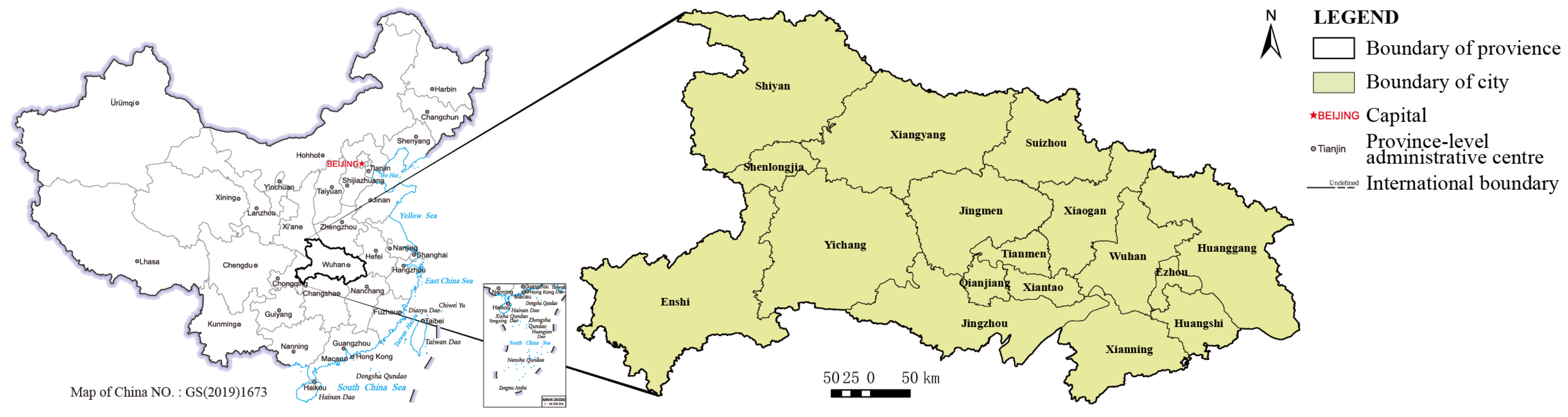
2.1. Study Area

Hubei Province is located in central China (31°12′ N 112°18′ E), with an area of approximately 185,900 km2, and features a subtropical monsoon climate (Figure 1). As a key participant in China’s “Rise of Central China” strategy, the advantageous geographic position of Hubei Province enables it to drive the regional economy forward. Nevertheless, the rapid development of the economy, social production, and consumption activities also led to a sharp rise in carbon emissions. Therefore, Hubei Province plays a pivotal role as an early adopter of low-carbon development initiatives in response to the mounting pressures and responsibilities for reducing carbon emissions.
This study utilized multiple datasets, including spatial and statistical data for every 5 years from 2000 to 2020 (Table 1). The spatial datasets included land use and land cover change (LUCC), normalized difference vegetation index (NDVI), land surface temperature (LST), visible infrared imaging radiometer suite (VIIRS), population (POP), gross domestic product (GDP), road, and particulate matter PM2.5 (PM) data. The statistical data comprised nine different fossil fuels from the Hubei Provincial Statistical Yearbook (Table 2). In addition, green cover impacts (GCI) and blue cover impacts (BCI) were calculated as the ratio of green/blue space per kilometer. The degree of urbanization (DU) was calculated based on the share of the local population residing in urban clusters and urban centers. The secondary sector level (2Sector) represented the share of secondary industry in GDP. The industrial scale (IS) was determined based on the proportion of industrial land per 1 km. All data were resampled in GIS (ArcGIS 10.3) using the WGS_1984 coordinate system with a pixel resolution of 1 km × 1 km. Missing values in spatial datasets (e.g., LUCC and NDVI) were identified using quality assessment bands (e.g., MODIS QA layers) and interpolated via nearest neighbor imputation in ArcGIS for continuous rasters. Missing annual values in statistical data (e.g., GDP and population) were filled using linear interpolation based on temporal trends, with reference to adjacent years’ data in the Hubei Provincial Statistical Yearbook. All data at 30 m resolution were resampled to match the LUCC coordinate system using bilinear interpolation.

2.2. Net Carbon Emissions Calculation

The calculation of net carbon emissions involves determining the difference between carbon emissions and sinks [31,32,33]. Achieving carbon neutrality occurs when the net carbon emissions value is zero, meaning that carbon emissions and carbon sinks are equal. Carbon sinks are mainly calculated as the amount of CO2 absorbed by woodland, grassland, water, and unused land. Carbon emissions, on the other hand, are calculated as CO2 emissions from construction land and industrial land. Although farmland has been proven by different researchers to be either a carbon sink or a source of emissions in different cities, this depends on factors such as crop types and farming practices [34]. However, the results of long-term studies show that farmland in Hubei Province generally shows a trend of being carbon sinks [35]. While cropland carbon flux dynamics are influenced by complex interactions between crop rotation patterns, agricultural management practices, and climate extremes, this study employs a conservative methodology grounded in historical trend analysis to classify these agricultural systems as net carbon sinks.

2.2.1. Calculation of Carbon Sinks

Woodland, grassland, farmland, water, and unused land exhibit relatively stable environmental changes over a long period of time. Most research uses the coefficient method for carbon sink calculations, with the following formula:
C a b s o r b = ( S i × a i )
where, C a b s o r b represents the total number of carbon sinks. S i denotes the area of LUCC type i . a i represents the carbon sink coefficient for LUCC type i . According to research conducted by Fang, et al. [36], Duan, et al. [37], Lai [38], Zhang, et al. [39], and Zhang, et al. [40], the carbon sink coefficients for woodland, grassland, farmland, water, and unused land in Hubei Province are −5.77 t·hm−2, −0.022 t·hm−2, −0.13 t·hm−2, −0.298 t·hm−2, and −0.005 t·hm−2, respectively.

2.2.2. Calculation of Carbon Emissions

The carbon emissions from construction and industrial land mainly result from energy consumption associated with human activities [41,42]. Considering the large differences in economic and social development levels among the cities in Hubei Province, using the coefficient method for carbon emission calculations could lead to substantial errors. Therefore, we choose to consult the IPCC Guidelines for National Greenhouse Gas Emission Inventories, which consider the carbon emissions from energy consumption for the calculation of carbon emissions from construction land and industrial land.
C e m i s s i o n = e i = E i × b i × θ i
where i represents the type of fossil fuels (i.e., raw coal, coke, crude oil, gasoline, kerosene, diesel, fuel oil, natural gas, and electricity in Table 2). C e m i s s i o n refers to the total amount of carbon emissions. e i denotes the specific amount of carbon emissions from fuel i . E i represents the consumption of fuel i . b i indicates the standard coal conversion factor for fuel i . θ i represents the carbon emission coefficient of fuel i . The standard coal conversion coefficients for each energy source are obtained from the China Energy Statistics Yearbook, while the carbon emission coefficients are sourced from the IPCC Guidelines for National Greenhouse Gas Inventories.

2.2.3. Calculation of Net Carbon Emissions

The net carbon emissions are derived by calculating the total difference between carbon emissions and carbon sinks for all land use types. The formula is as follows:
C t o t a l = C e m i s s i o n   C a b s o r b  
where C t o t a l represents the total amount of net carbon emissions. C e m i s s i o n denotes the total amount of carbon emissions. C a b s o r b signifies the total amount of carbon sinks.

2.3. Spatial and Temporal Distribution of Net Carbon Emissions

The land use changes of woodland, grassland, farmland, water, and unused land were calculated based on the satellite maps of LUCC at 5-year intervals between 2000 and 2020. Due to the lack of reliable data on the spatial distribution of CO2 emissions from construction and industrial land at the city level in Hubei Province, this study used night-time light maps to indirectly estimate the distribution of carbon emissions due to the strong correlation between them [43]. Firstly, we derived a fitting equation by establishing the relationship between night-time lighting data and carbon emissions from energy consumption in cities in Hubei Province in the corresponding years. Afterward, this equation was used to generate the spatial distribution of CO2 emissions from construction and industrial land. The multiple regression equations were chosen as the fitting model (Table 3). The results showed that there was a strong correlation between night-time lighting data and carbon emissions (with an average R2 value above 0.80); thus, this method could be used in this study to map the spatial distribution of carbon emissions from construction and industrial land in Hubei Province.

2.4. Assessment of Net Carbon Emissions with Influencing Factors

Based on previous research findings, five different indicators were selected to describe the environmental conditions, including the normalized difference vegetation index (NDVI), blue cover impacts (BCI), green cover impacts (GCI), PM2.5 (PM), and land surface temperature (LST). On the other hand, economic conditions are represented by secondary sector level (2Sector), population (POP), degree of urbanization (DU), road density (RD), industrial scale (IS), and gross domestic product (GDP), which reflect the level of development within the city (Table 4).
Firstly, we pre-processed all the data. Considering the different units and value ranges of the various influencing factors, which could affect the results to some extent, we normalized all the data using normalization. We employed the min–max normalization method for pre-processing raw data, primarily based on two key considerations. First, compared to z-score standardization, the min–max approach preserves the original data distribution characteristics through linear transformation mapping to the [0,1] interval, which is particularly crucial for subsequent spatial pattern analysis. Second, the dataset exhibits significant spatial heterogeneity, manifested as high sparsity (i.e., abundant zero-value distributions) in carbon emission/sequestration metrics between built-up and non-built-up areas. When applying z-score standardization, these extreme sparse characteristics tend to cause standard deviations approaching zero, thereby inducing numerical calculation distortion. This distinct spatial heterogeneity ensures that min–max normalization not only eliminates dimensional influences but also more robustly maintains data distribution patterns, thereby providing a reliable data foundation for subsequent spatial modeling. We used Excel to calculate all normalization processes. Secondly, we spatially mapped all the data. All datasets were imported into ArcGIS with a precision of 1 km, resulting in a total of 184,650 datasets with a spatial precision of 1 km × 1 km. Thirdly, we employed machine learning techniques to assess the performance of different regression models in correlating the influencing factors with net carbon emissions in Hubei Province, aiming to identify the most suitable model for subsequent analyses. We used ten different machine learning models, including linear regression, polynomial linear regression, ridge, lasso, decision tree regression, SVR, random forest regressor, XGB regressor, KNeighbors, and elastic net. The primary goal of the regression task was to model the relationship between 11 influencing factors and net carbon emissions, with the aim of identifying the key factor(s). To optimize the fitting results and prevent overfitting, we divided the dataset into a training set and a test set in a ratio of 4:1. We performed comprehensive hyperparameter optimization for each machine learning model through a systematic grid search strategy. Key parameters subjected to optimization included ensemble size (n_estimators: 50–500), tree depth constraints (max_depth: 10–100), node splitting criteria (min_samples_split: 2–10), and leaf node requirements (min_samples_leaf: 1–5). Model optimization employed 5-fold cross-validation with stratified sampling to ensure robust generalization capability evaluation, incorporating early stopping mechanisms to prevent overfitting. The configuration process focused on minimizing the root mean squared error (RMSE) metric on validation data, with parallel computing implementation accelerating the search across the parameter hyperspace. Finally, Shapley additive explanations (SHAP), a game-theoretic approach used to explain the output of any machine learning model, was used to interpret the weight of different influencing factors. The greatest advantage of SHAP lies in its capability to reflect the influence of each feature in every sample, reveal whether the influence is positive or negative, and provide powerful data visualization functions [44]. All models were implemented in Python (version 3.10).

3. Results and Analysis

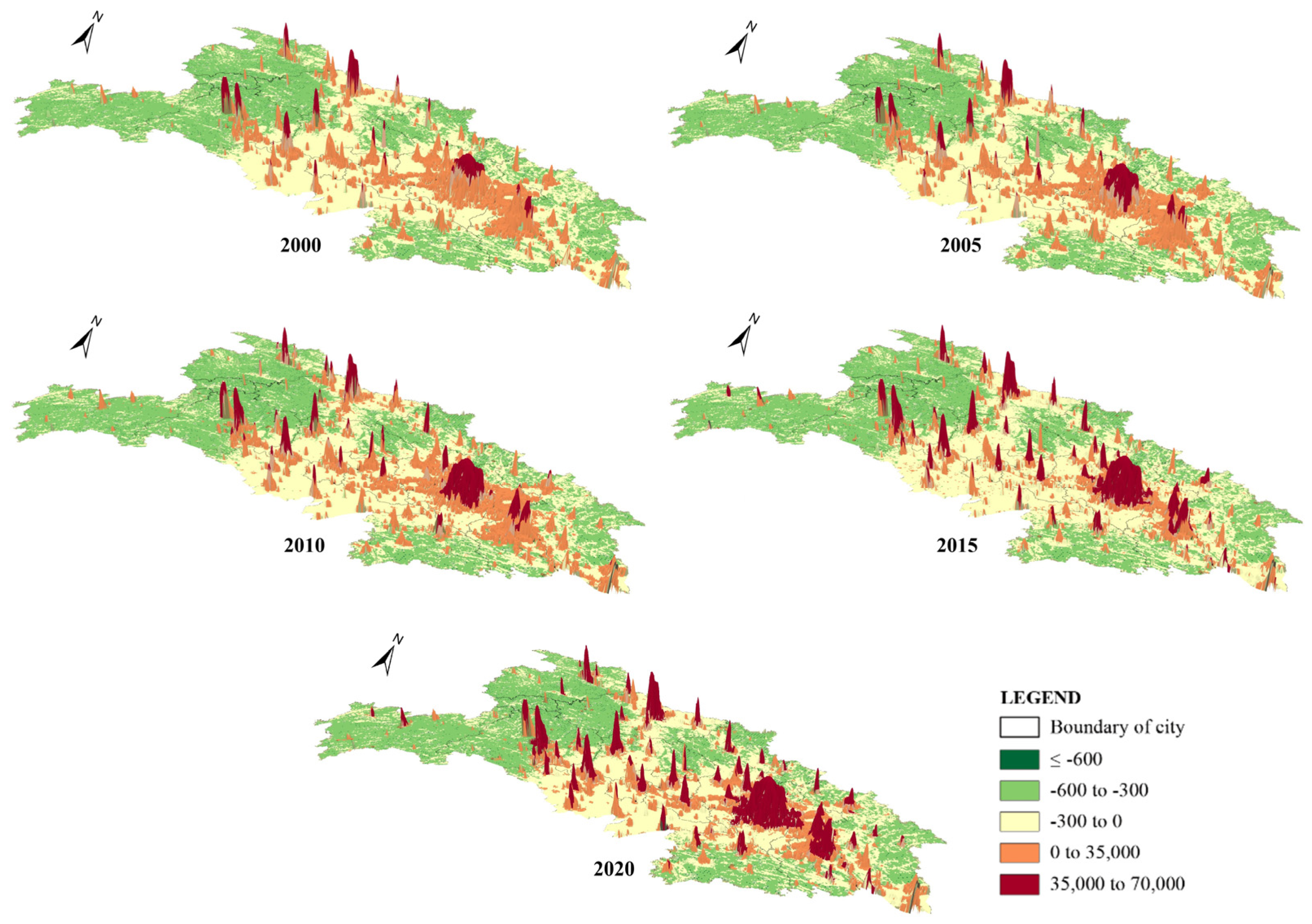
3.1. Spatial and Temporal Changes in Land Use Patterns and Net Carbon Emissions

The net carbon emissions from different land use types in Hubei Province were calculated for different time periods (Table 5). Overall, carbon emissions in Hubei Province show an upward trend, with total net carbon emissions rising from 8.3 × 10¹⁰ kg in 2000 to 25.0 × 10¹⁰ kg in 2020. The net emissions in the study area are consistently positive, indicating that the study area overall acts as a carbon + source. Among all LUCC types, woodlands serve as the primary carbon sink source in Hubei Province, absorbing an average of 97.7% of the total provincial carbon sinks. However, the carbon sink capacity of woodlands has been on a gradual decline, with values of 5.34 × 10¹⁰ kg (2000), 5.34 × 10¹⁰ kg (2005), 5.34 × 10¹⁰ kg (2010), 5.32 × 10¹⁰ kg (2015), and 5.31 × 10¹⁰ kg (2020) in different years. Farmland is the second most significant carbon sink source among the LUCC types. The decline in woodland carbon sinks (a reduction of 35.1 × 10⁷ kg from 2000–2020) stems from multiple interconnected factors. Satellite-derived LUCC data (Figure 2) reveal a big reduction in woodland areas in urban core zones (e.g., Wuhan and Huangshi) over the period, primarily driven by urban sprawl and industrial park development. Additionally, selective logging and conversion to commercial forest plantations (e.g., tea gardens and eucalyptus) in mountainous regions (e.g., Enshi) reduced forest carbon density. On the other hand, construction land and industrial land, which continue to increase carbon emissions, are the main sources of carbon emissions in Hubei Province. While carbon emissions from construction land soared from 12.2 × 10¹⁰ kg in 2000 to 127.1 × 10¹⁰ kg in 2020, their share of total carbon emissions declined from 88.7% in 2000 to 56.2% in 2020. Conversely, the proportion of total carbon emissions attributable to industrial land increased from 11.3% in 2000 to 43.8% in 2020.
Using the natural breakpoint method via ArcGIS, we systematically categorized the net carbon emissions in Hubei Province from 2000 to 2020 into five distinct classes (Figure 2). The spatial analysis reveals a pronounced disparity in net carbon emissions, with elevated levels in the eastern and southern sectors of the study area and markedly lower emissions in the western and northern regions. Specifically, the “Wuhan Metropolitan Area”, characterized by its robust secondary industry, emerged as the major contributor to net carbon emissions in the study area, with Wuhan and Huanggang at the epicenter of this contribution. The “Yijing Jing’en Urban Agglomeration” closely follows, with Jingzhou City leading in emissions within this cluster. In contrast, Shennongjia and Enshi are the only cities in Hubei Province with negative net carbon emissions and are among the few carbon sink cities.
In terms of historical changes, the overall trend in the spatial pattern of net carbon emissions within the study area displays concentric rings that progressively expand outward. In 2000, the net carbon emissions in the study area showed a point-like pattern, with higher emissions mainly observed in Wuhan and its neighboring cities. By 2005, this pattern had evolved into a clustered distribution, with Wuhan and Xiangyang serving as the central nodes of carbon emission aggregation. From 2010 onwards, the emission dynamics transitioned from a singular centralized concentration to a complex, multi-nodal configuration, including Xiangyang and Yichang. This shift reflects a more balanced approach to economic development and resource utilization across the study area. By 2020, the pattern of net carbon emissions had further matured into a configuration characterized by a weak center, a strong central ring, and a moderate outer ring. In contrast to Hubei Province, Henan Province (located in central China with a similar industrial structure) exhibits a comparable east–west emission gradient, with high emissions in the industrialized eastern plains (e.g., Zhengzhou) and lower emissions in the mountainous western Funiu Range [45]. This aligns with Hubei’s east–south dominance, driven by urban agglomerations (Wuhan Metropolitan Area) and industrial corridors. In contrast, Sichuan Province (located in western China with more balanced urban–rural development) shows a clustered emission pattern concentrated in the Chengdu–Chongqing conurbation, with less pronounced regional disparity than Hubei’s stark east–west divide [46].

3.2. Assessment of Net Carbon Emissions

3.2.1. Performance Comparison of Different Machine Learning Models

We used a series of machine learning models to comprehensively analyze the relationship between different influencing factors and net carbon emissions in Hubei Province. The performance of these models was assessed using the root mean square error (RMSE) and mean absolute error (MAE) metrics (Table 5). Using the SNAP function of ArcGIS, Hubei Province was divided into 184,650 squares with a size of 1 km × 1 km. Each square contains 10 influencing factors and net carbon emissions data. The dataset was divided into training sets (80%) and testing sets (20%) in a ratio of 4:1 to apply machine learning techniques and determine the most appropriate regression model. As shown in Table 6, the XGB regressor (XGB) has the worst regression performance, with RMSE values of 0.576 and 1.171 and MAE values of 0.418 and 0.686 for the training and test sets, respectively. This anomaly contrasts with XGBoost’s typical superiority in regression tasks, suggesting potential causes such as inadequate hyperparameter tuning (e.g., learning rate and max_depth), improper handling of missing values, or data scaling issues [47]. Support vector regression (SVR) also underperformed (RMSE of 0.094), which is attributable to its sensitivity to parameters within the kernel function, which makes it more suitable for classification tasks.
By comparing the linear regression and polynomial regression models, it can be found that the latter performs significantly better than the former based on the training and test sets. This suggests that there may be a complex nonlinear relationship between influencing indicators and net carbon emissions, and thus the polynomial regression model is able to fit this relationship better compared to the linear regression model. However, regularized linear regression models did not show better performance compared to linear regression models (i.e., ridge regression and elastic net regression). Their RMSE values based on the training and testing sets were worse than those of the linear regression models. This may be due to the default settings of explanatory variables being first-order terms, which do not leverage the advantage of regularized models in addressing multicollinearity issues in polynomial regression. Additionally, decision tree regression (DTR) achieved near-zero training errors (RMSE = 0, MAE = 0) but maintained moderate generalization (test RMSE = 0.05). While DTR’s spatial interpretability is advantageous for grid-based analysis, its perfect training fit indicates severe overfitting, making it unsuitable for subsequent SHAP interpretation.
The random forest regression (RFR) model demonstrated the greatest performance and excellent generalization compared to the other machine learning models, especially in the model optimized with random search. From the fitting results of the training and testing sets, the RMSE value of RFR is lower than 0.02, and the MAE value is also the lowest among all models. These results indicate that RFR not only performs well but also has outstanding generalization ability. The results of K-CV cross-validation are consistent with the analysis based on RMSE and MAE. In conclusion, the RFR regression was selected as the basis of the SHAP interpretation for exploring and analyzing the key influencing factors affecting net carbon emissions.

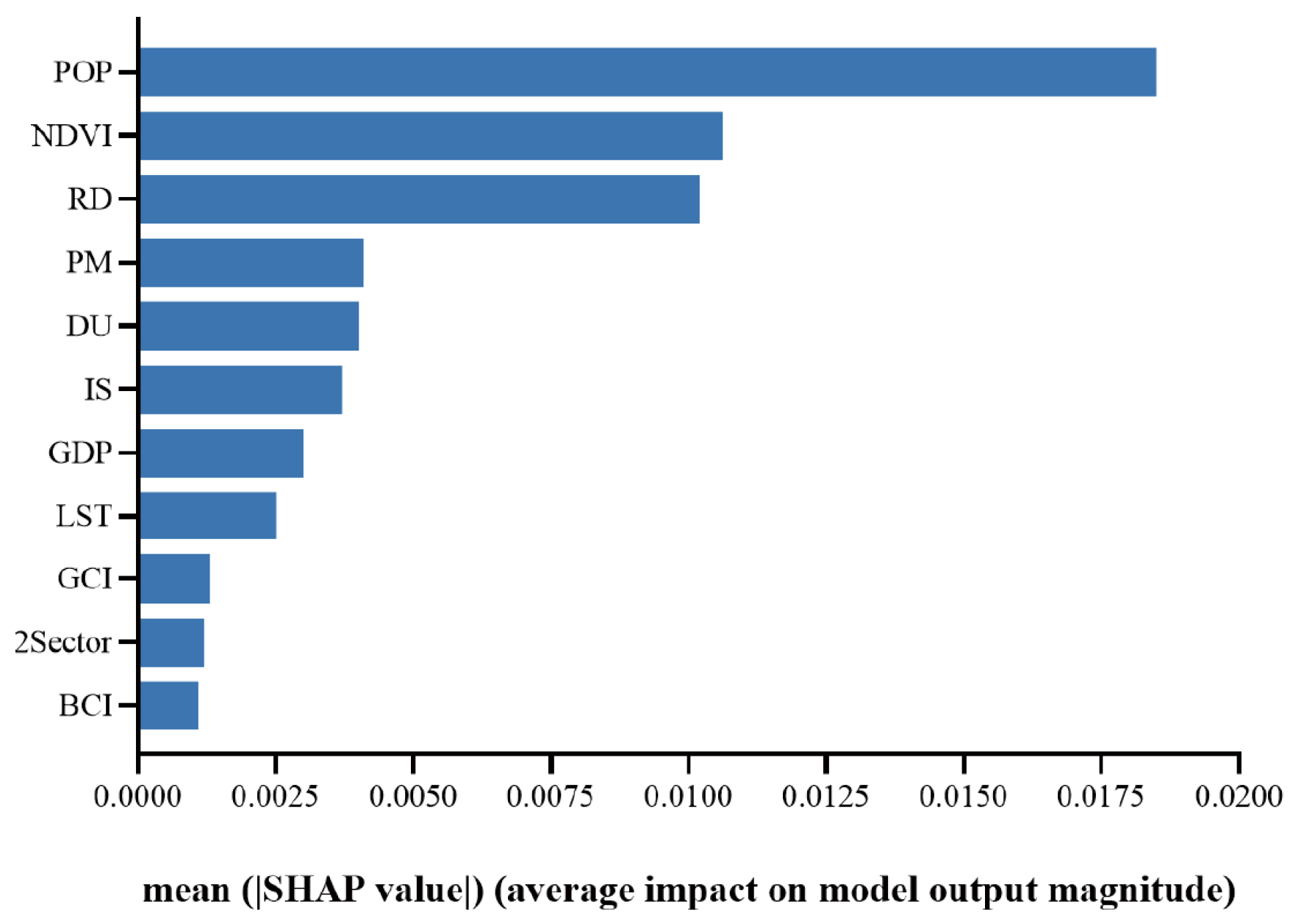
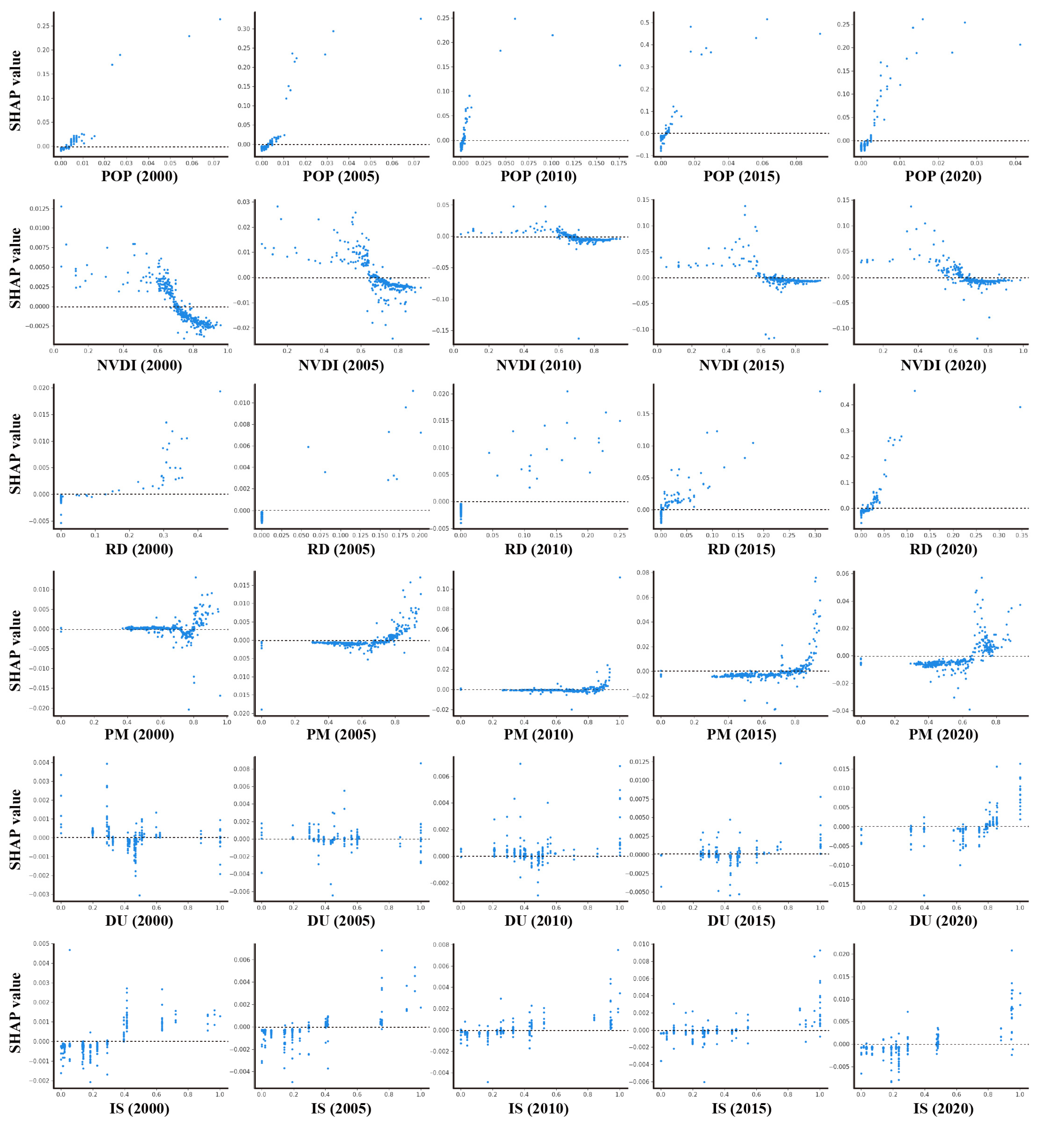
3.2.2. SHAP Interpretation Based on RFR Model

Based on the results of the RFR model, we calculated the SHAP values for each input feature in the testing set (Figure 3 and Figure 4), as well as the SHAP interaction values (Figure 5). The six key factors that have the greatest impact on net carbon emissions in Hubei Province are population (POP), the normalized difference vegetation index (NDVI), road density (RD), PM2.5 (PM), degree of urbanization (DU), and industrial scale (IS) (Figure 3). This result is similar to the results of previous studies on low-carbon transition, which generally agree that population, vegetation, and degree of urban development are the main influencing factors [48,49,50]. However, our results also suggest that we should pay more attention to the impacts of road density, especially the destruction of natural forests by roads and their potential impacts on net carbon emissions.
Figure 4 illustrates the distribution of SHAP value trends (i.e., SHAP dependency plot) for nine different factors affecting net carbon emissions in Hubei Province. We observe that POP, PM, DU, 2Sector, and GDP demonstrate upward trends, suggesting that increases in these factors are associated with higher net carbon emissions in the region. Among these, POP shows the most significant upward trend, indicating that population growth has a substantial impact on net carbon emissions relative to other factors. DU and 2Sector show milder upward trends, implying that moderately controlling urban development rates can help mitigate net carbon emissions through the promotion of balanced urban growth across Hubei Province. Conversely, only the NDVI shows a decreasing trend, with a narrowing distribution of observation points. This suggests that although plants can help reduce net carbon emissions by absorbing CO2, their impact is limited when NDVI values fall below the average. However, a significant reduction in net carbon emissions is only observed when NDVI values exceed approximately 70%.
Based on the SHAP feature importance map (Figure 3), we selected the top six key factors for further comparative analysis for every five years between 2000 and 2020 (Figure 5). However, these findings show discrepancies compared to analyses from other cities in China. In coastal cities and Sichuan Province, for instance, GDP consistently emerges as a statistically significant factor in carbon emission studies [51,52]. Enhanced economic development in these areas enables governments to strengthen fiscal capacities for technological advancement and implement ecosystem protection/restoration projects, thereby promoting ecological function recovery and carbon sink capacity enhancement. However, in Hubei Province, economic investments predominantly prioritize urban infrastructure development. Jiangsu Province demonstrates a distinct pattern of industrial evolution. Against the backdrop of gradually moderating economic growth rates compared to Hubei, the secondary industry (predominantly manufacturing) has progressively become the core driver of regional economic growth. This industrial restructuring has led to the persistent weakening of the economic scale’s influence on carbon emissions, while the marginal effect of industrial structure optimization on emission patterns has significantly intensified [53].
(1) Population (POP): The impact of population density on net carbon emissions has gradually increased over time. As observed in the SHAP dependency plot, the trend slope angle of the SHAP value for POP increased from 45° to approximately 70°. This steeper slope indicates a more significant increase in net carbon emissions at the same population density levels. Although the actual and normalized values of population density (approximately 57 million and 0.02, respectively) remained similar between 2000 and 2020, the fourfold difference in the SHAP value of POP over this period signifies a substantial rise in net carbon emissions in areas of high population density (Figure 4). This finding contrasts with other studies that suggest reducing carbon emissions by increasing urban population density to decrease transportation costs [54].
We also found that the instances of negative SHAP values were more prevalent in 2020 than in 2000, accounting for an increase from 20% to 70%. This trend suggests that areas with lower population density generated fewer net carbon emissions in 2020 compared to 2000, potentially due to a series of policies such as the long-term ban on straw-burning and the adoption of cleaner energy sources (e.g., natural gas) in the construction of “new rural districts” by the government in the last 20 years. In summary, Hubei Province should prioritize addressing high carbon emissions in densely populated areas (e.g., urban centers) while maintaining the significant improvements already achieved in rural areas.
(2) The normalized difference vegetation index (NDVI) is a simple numerical indicator and a powerful tool that is used to assess spatio-temporal changes in green vegetation [55,56]. In 2000, the trend of the SHAP value for the NDVI was nearly at a 45-degree angle, indicating that healthy vegetation communities in Hubei Province were initially effective in suppressing the increase of net carbon emissions. By 2020, however, the SHAP curve for the NDVI gradually flattened, and the SHAP value approached zero as the NDVI increased. This indicates that the inhibitory effect of the NDVI on net carbon emissions is gradually weakening, and net carbon emissions have exceeded the maximum absorption potential of vegetation. Without additional methods, such as increasing the vegetation area and enhancing management, the current vegetation in Hubei Province plays a limited role in reducing overall net carbon emissions. For instance, in sustainable road planning and design strategies, brownfield redevelopment should be prioritized through existing infrastructure utilization over greenfield expansion to reduce the conversion of forested and agricultural lands. For urban vegetation management, strict land use controls should be implemented to preserve mature high-carbon storage forests in peri-urban areas, exemplified by protected zones such as the Shennongjia Nature Reserve. Regarding economic forestry optimization, there should be a transition from short-rotation monoculture plantations (e.g., fast-growing eucalyptus) to perennial multi-functional species (e.g., oil tea camellia) that maintain belowground carbon reserves through extended root system preservation. Furthermore, we found that until the plant cover density reaches a certain scale (e.g., a standardized value of about 0.6), this vegetation can even become a burden on carbon emissions in the region. By manually calibrating satellite images, we discovered that parts of these areas consist of young woodlands, which are either economic forests or fallow forests. This phenomenon may be due to the growth demands of young plants, which result in greater respiration than photosynthesis, thereby generating a large amount of carbon emissions [57].
(3) Road density (RD) quantifies the total length of the road network relative to the geographic area of a given region. This metric serves as a crucial gauge for assessing the sophistication of urban road networks [58]. The influence of RD on net carbon emissions mirrors the patterns observed with population density (POP), both in intensity and trajectory. Notably, as RD escalates, its effect on carbon emissions intensifies, a trend that has become more distinct over the years. This is clearly illustrated by the trend line’s increasing slope, which has steepened from approximately 20° in 2000 to about 60° in 2020. Secondly, the trend in RD’s SHAP value evolved from an L-shape in 2000 to a linear pattern by 2020. This transformation suggests that initially, there was a lack of effective segregation between high-emission industrial facilities and residential zones within the urban core. Historically, regions with robust industrial development have attracted denser populations, which in turn spiked carbon emissions once the population—and correspondingly, RD—reached critical thresholds. This indicates a strong interdependence between urban planning and environmental impact. However, by 2020, through the implementation of targeted environmental strategies such as the relocation of polluting factories and the green transformation of industries, these emissions sources were more uniformly distributed across different levels of road density. This strategic dispersion has mitigated the localized spikes in emissions that were previously observed. Moreover, when RD remains low (with a normalized value around 0.02), it does not exacerbate net carbon emissions. This observation underscores that enhancing basic road infrastructure in economically disadvantaged areas within Hubei Province, such as ensuring that each village has at least one hardened road, does not inherently increase the burden of achieving carbon neutrality. This research provides critical insights for policymakers seeking to reconcile infrastructure expansion with climate mitigation imperatives. Particularly in high-emission southeastern regions such as the Wuhan Metropolitan Area, urban planning authorities should prioritize the implementation of compact development strategies to mitigate transport-related emissions through optimized road network configurations.
(4) PM2.5 (PM) denotes the concentration of dust or drifting dust particles with a diameter of 2.5 μm or less in ambient air [59]. This measurement is a crucial indicator used by environmental authorities in many countries to monitor atmospheric pollution. Figure 5 further reveals dynamic interactions between key factors over time. For PM, the SHAP value distribution in 2000 shows a bimodal pattern, with low-impact clusters at normalized values <0.5 and high-impact clusters >0.8, reflecting the limited industrial pollution at the turn of the century. By 2020, the high-impact tail expands significantly, indicating that PM concentrations in more regions have exceeded the threshold (normalized value >0.8), where they strongly correlate with carbon emissions. This aligns with Hubei’s industrial expansion, particularly in the steel, cement, and chemical sectors, which emit both PM and CO2. Notably, cities such as Wuhan and Huangshi, with historically high PM levels, exhibit SHAP values 2–3 times higher in 2020 than in 2000, underscoring the need for integrated air quality and carbon control policies. Given the hazardous effects of PM in triggering respiratory and cardiovascular diseases, the government could prioritize addressing areas with high levels of both PM and CO2 in its energy conservation and emission reduction strategies. This approach would yield greater social value by not only mitigating environmental pollution but also enhancing public health.
(5) The degree of urbanization (DU) represents the proportion of the urban population compared to the total population and serves as a primary measure of urbanization [60]. The SHAP dependency plot evolves from a negative-to-positive trend. Specifically, lower DU areas experienced higher carbon emissions in 2000. According to the spatial distribution map of carbon emissions (Figure 4), high carbon emissions were mainly concentrated in Wuhan, Ezhou, and Huangshi. This phenomenon can be attributed to the limited size of urban areas at the time, with most industrial facilities located in suburban regions. The conversion of farmland into industrial land in these areas led to significant migration of the rural population into urban centers, causing substantial carbon emissions even though the normalized urbanization rate was close to zero. As the value of DU rates increased, most regions exhibited a suppressive effect on carbon emissions. This trend is related to the disparities in the development levels of cities within Hubei Province, with high carbon-emitting industries concentrated in a few developed cities. However, after 2020, the situation reversed. High DU values began to contribute to increased net carbon emissions. This shift can be attributed to urban expansion and the migration of large populations from rural to urban areas. As cities expanded, industrial zones previously located in rural areas became part of the urban space.
However, after 2020, the situation reversed. High DU values began to contribute to increased net carbon emissions. This shift can be attributed to urban expansion and the migration of large populations from rural to urban areas. As cities expanded, industrial zones previously located in rural areas became part of the urban space. Additionally, the increase in the urban population led some people to move to areas further from the urban center, where housing prices are lower. These factors combined to significantly increase the impact of DU on net carbon emissions. Furthermore, we observed that cities with normalized DU values below 0.7 had a dampening effect on net carbon emissions. In other words, the top 30% of areas with the highest DU values were the main contributors to net carbon emissions in Hubei Province, which is consistent with the observations from the spatial distribution map of carbon emissions (Figure 4).
(6) Industrial scale (IS) measures the proportion of the secondary sector’s output in the gross national product. It has a progressively positive impact on net carbon emissions (Figure 5). Specifically, the slope of the IS trend in the SHAP dependency graph steepens from about 10° in 2000 to approximately 40° in 2020, indicating that regions with comparable levels of industrialization emitted significantly more carbon in 2020 compared to 2000. In regions where the standardized value of IS is near 1, indicating a high concentration of secondary industries, the SHAP value in 2020 is tenfold that of 2000, suggesting that industrial groups have scaled up and are emitting substantially more carbon than in the past. However, according to the Hubei Provincial Bureau of Statistics [61], the proportion of the secondary sector in the GDP has only slightly declined by about 0.7%, from 40.5% (CNY 143,738 million) in 2000 to 39.8% (CNY 170,239 million) in 2020. This modest decline suggests that the observed increase in carbon emissions may be attributed to the lack of optimization in some industrial units and the strategic industry layout designed to meet the diversified demand for industrial products in Hubei Province, which may inherently have higher carbon footprints. Notably, the interaction between IS and road density (RD) strengthens over time. In 2000, regions with high IS but low RD (e.g., isolated industrial parks) show limited emission impacts, while by 2020, the same IS levels in high-RD areas (well-connected industrial corridors) exhibit nearly 50% higher SHAP values. This suggests that improved transportation networks facilitate industrial logistics but also amplify carbon footprints, a nuance that is critical for low-carbon urban planning.
It is worth noting a couple of limitations to this study. First, the VIIRS-based night-time light proxy methodology demonstrates inherent limitations in emission source representation. Animal husbandry and transportation systems remain inadequately captured due to their low correlation with artificial lighting intensity. This may underestimate the carbon emissions in rural areas. Secondly, the classification of farmland as a consistent carbon sink overlooks seasonal and management-induced variations. Future research could incorporate high-frequency monitoring data and perform sensitivity analyses (e.g., varying farmland carbon coefficients or light emission regression models) to quantify uncertainties and enhance the robustness of estimates.

4. Conclusions

This study primarily focuses on analyzing the relationship between net carbon emissions and various influencing factors in Hubei Province, including land use, energy consumption, night lighting data, and economic data such as population and GDP from 2000 to 2020. Through the utilization of a machine learning model and the SHAP algorithm, we fitted the relationship between net carbon emissions and identify key factors in Hubei Province. The main findings of this research are as follows:
(1) Net carbon emissions in Hubei Province exhibit a consistent upward trend from 2000 to 2020. Net carbon emissions increased from 8313.02 × 107 kg in 2000 to 25,047.57 × 107 kg in 2020. This represents an overall growth rate of 201.3%, with an average annual increase of approximately 10.1%. Among the contributors, construction land accounts for the largest share of net carbon emissions, comprising 56.2% of the total in 2020. Industrial land exhibits the highest growth rate in carbon emissions, with a remarkable increase of 755.9% over the past 20 years. Conversely, woodland contributes the most to carbon sinks, but has seen a reduction in CO2 uptake by 35.1 × 10⁷ kg in these 20 years. Net carbon emissions from other land use categories have remained relatively stable.
(2) The SHAP interpretation identifies six key factors that affect net carbon emissions in the study area. These are population (POP), the normalized difference vegetation index (NDVI), road density (RD), PM2.5 (PM), the degree of urbanization (DU), and industrial scale (IS). These factors have varying impacts on cities with different levels of development across the province. Notably, as the values of these influencing factors increase, five of the key factors—excluding NDVI—contribute to higher net carbon emissions.
(3) Significant regional differences in net carbon emissions exist in the study area due to variations in landform, natural resources, economic development stages, and urban boundaries across different regions. Over time, areas with high carbon emissions have spread from the provincial capital to neighboring cities. From 2000 to 2020, net carbon emissions in Hubei Province exhibited a spatial distribution pattern characterized by higher emissions in the east and south and lower emissions in the west and north, forming a ring-shaped pattern of gradual outward dispersion.
(4) Net carbon emissions in the study area show obvious spatial aggregation characteristics. Net carbon emissions are mainly concentrated in the central areas of counties in Hubei Province, and there is a significant difference in carbon emissions between urban and rural areas. Regions with standardized values higher than 0.8 contribute the most net carbon emissions. This is because the people and industries are mainly concentrated in urban areas, resulting in much higher fossil energy consumption than in rural areas.
(5) The six key factors exhibit context-dependent impacts. Population growth drives emissions in dense urban cores but correlates with lower emissions in rural areas post-2020 due to policy interventions. The NDVI’s diminishing marginal effect indicates that vegetation carbon sinks in Hubei are approaching saturation, necessitating the afforestation of mature forests rather than young saplings. The synergistic increase in road density and industrial scale highlights the trade-off between economic connectivity and carbon efficiency. These nuances imply that carbon neutrality strategies should be differentiated by region: stricter industrial emission controls in high-DU cities, targeted greening of urban peripheries, and low-carbon transportation networks in emerging industrial corridors.

Author Contributions

Writing—original draft; Funding acquisition; Methodology; Project administration, J.Z. Software; Writing—original draft, B.J. Supervision; Writing—review and editing; Funding acquisition, J.W. Data curation; Visualization, X.W. All authors have read and agreed to the published version of the manuscript.

Funding

This research was supported by the Natural Science Foundation of Hubei Province (Grant No. 2025AFC008), The Young Top-notch Talent Cultivation Program of Hubei Province (Grant No. 2021 Frist Batch), and the MOE (Ministry of Education in China) Liberal arts and Social Sciences Foundation (Grant No. 22YJA760086).

Data Availability Statement

The raw data supporting the conclusions of this article will be made available by the authors on request.

Acknowledgments

The authors gratefully acknowledge Dawei Li (Sun Yat-sen University, China) for her technical guidance in conducting this study.

Conflicts of Interest

The authors declare no conflicts of interest.

References

  1. Liu, J.; Shao, Q.; Yan, X.; Fan, J.; Deng, X. An Overview of the Progress and Research Framework on the Effects of Land Use Change upon Global Climate. Adv. Earth Sci. 2011, 26, 1015. [Google Scholar]
  2. IPCC. Climate Change 2014: Impacts, Adaptation and Vulnerability. Contribution of Working Group II to the Fifth Assessment Report of the Intergovernmental Panel on Climate Change; Cambridge University Press: Cambridge, UK; New York, NY, USA, 2014. [Google Scholar]
  3. Goldewijk, K.K.; Ramankutty, N. Land cover change over the last three centuries due to human activities: The availability of new global data sets. GeoJournal 2004, 61, 335–344. [Google Scholar] [CrossRef]
  4. Houghton, R.A. The annual net flux of carbon to the atmosphere from changes in land use 1850–1990. Tellus Ser. B-Chem. Phys. Meteorol. 1999, 51, 298–313. [Google Scholar] [CrossRef]
  5. Tang, X.; Woodcock, C.E.; Olofsson, P.; Hutyra, L.R. Spatiotemporal assessment of land use/land cover change and associated carbon emissions and uptake in the Mekong River Basin. Remote Sens. Environ. 2021, 256, 112336. [Google Scholar] [CrossRef]
  6. Björkegren, A.; Grimmond, C.S.B. Net carbon dioxide emissions from central London. Urban Clim. 2018, 23, 131–158. [Google Scholar] [CrossRef]
  7. Jiang, X.; Chen, Q.; Guan, D.; Zhu, K.; Yang, C. Revisiting the global net carbon dioxide emission transfers by international trade: The impact of trade heterogeneity of China. J. Ind. Ecol. 2016, 20, 506–514. [Google Scholar] [CrossRef]
  8. Houghton, R.A.; House, J.I.; Pongratz, J.; Van Der Werf, G.R.; Defries, R.S.; Hansen, M.C.; Ramankutty, N. Carbon emissions from land use and land-cover change. Biogeosciences 2012, 9, 5125–5142. [Google Scholar] [CrossRef]
  9. Wang, S.; Fang, C.; Wang, Y.; Huang, Y.; Ma, H. Quantifying the relationship between urban development intensity and carbon dioxide emissions using a panel data analysis. Ecol. Indic. 2015, 49, 121–131. [Google Scholar] [CrossRef]
  10. Dong, J.; Yuan, K.Q. Carbon emission from land use and its efficiency in hubei province. Bull. Soil Water Conserv. 2016, 36, 337–342+348. [Google Scholar]
  11. Li, J.; Mao, D.; Jiang, Z.; Li, K. Research on factors decomposition and decoupling effects of land use carbon emissions in Chang-Zhu-Tan Urban Agglomeration. Ecol. Econ 2019, 35, 28–34. [Google Scholar]
  12. Luo, F.; Guo, Y.; Yao, M.; Cai, W.; Wang, M.; Wei, W. Carbon emissions and driving forces of China’s power sector: Input-output model based on the disaggregated power sector. J. Clean. Prod. 2020, 268, 121925. [Google Scholar] [CrossRef]
  13. Yin, S.G.; Li, Z.J.; Song, W.X.; Ma, Z. Spatial differentiation influence factors of residential rent in Nanjing based on geographical detector. J. Clean. Prod. 2018, 20, 1139–1149. [Google Scholar]
  14. Lu, Z.; Yang, Y.; Wang, J. Factor decomposition of carbon productivity chang in china’s main industries: Based on the laspeyres decomposition method. Energy Procedia 2014, 61, 1893–1896. [Google Scholar]
  15. Hamadneh, T.; Batiha, B.; Gharib, G.M.; Montazeri, Z.; Dehghani, M.; Aribowo, W.; Eguchi, K. Candle Flame Optimization: A Physics-Based Metaheuristic for Global Optimization. Int. J. Intell. Eng. Syst. 2025, 18, 826–837. [Google Scholar]
  16. Hamadneh, T.; Batiha, B.; Gharib, G.M.; Montazeri, Z.; Dehghani, M.; Aribowo, W.; Eguchi, K. Perfumer Optimization Algorithm: A Novel Human-Inspired Metaheuristic for Solving Optimization Tasks. Int. J. Intell. Eng. Syst. 2025, 18, 633–643. [Google Scholar]
  17. Hamadneh, T.; Batiha, B.; Gharib, G.M.; Montazeri, Z.; Dehghani, M.; Aribowo, W.; Eguchi, K. Makeup Artist Optimization Algorithm: A Novel Approach for Engineering Design Challenges. Int. J. Intell. Eng. Syst. 2025, 18, 484–493. [Google Scholar]
  18. Hamadneh, T.; Batiha, B.; Gharib, G.M.; Montazeri, Z.; Dehghani, M.; Aribowo, W.; Ibraheem, I.K. Revolution Optimization Algorithm: A New Human-based Metaheuristic Algorithm for Solving Optimization Problems. Int. J. Intell. Eng. Syst. 2025, 18, 520–531. [Google Scholar]
  19. Hamadneh, T.; Batiha, B.; Gharib, G.M.; Montazeri, Z.; Werner, F.; Dhiman, G.; Eguchi, K. Orangutan optimization algorithm: An innovative bio-inspired metaheuristic approach for solving engineering optimization problems. Int. J. Intell. Eng. Syst. 2025, 18, 47–57. [Google Scholar]
  20. Li, D.; Liu, R.; Chen, D. Distribution characteristics of carbon emission by energy consumption in China as judged by spatial clustering analysis. J. Beijing Norm. Univ. (Nat. Sci.) 2013, 49, 529–533. [Google Scholar]
  21. Tu, Z.G.; Shen, R.J. Analysis on China’s carbon emission division and reduction path: Based on multivariate panel data clustering analysis method. J. China Univ. Geosci. (Soc. Sci. Ed.) 2012, 12, 7–13, 136. [Google Scholar]
  22. Zhou, J.; Wang, Y.; Liu, X.; Shi, X.; Cai, C. Spatial temporal differences of carbon emissions and carbon compensation in China based on land use change. Sci. Geogr. Sin 2019, 39, 1955–1961. [Google Scholar]
  23. Ding, B.; Yang, S.; Zhao, Y. Study on spatiotemporal characteristics and decoupling effect of carbon emission from cultivated land resource utilization in China. Land Sci. 2019, 33, 45–54. [Google Scholar]
  24. Lu, X.; Ota, K.; Dong, M.; Yu, C.; Jin, H. Predicting transportation carbon emission with urban big data. IEEE Trans. Sustain. Comput. 2017, 2, 333–344. [Google Scholar] [CrossRef]
  25. Shi, K. A Multiscale Analysis on Spatiotemporal Pattern of Carbon Emissions and Its Impact Factors in China Using DMSPOLS Data. Ph.D. Thesis, East China Normal University, Shanghai, China, 2017. [Google Scholar]
  26. Wang, S.; Fang, C.; Guan, X.; Pang, B.; Ma, H. Urbanisation, energy consumption, and carbon dioxide emissions in China: A panel data analysis of China’s provinces. Appl. Energy 2014, 136, 738–749. [Google Scholar] [CrossRef]
  27. Yan, H.; Guo, X.; Zhao, S.; Yang, H. Variation of net carbon emissions from land use change in the Beijing-Tianjin-Hebei region during 1990–2020. Land 2022, 11, 997. [Google Scholar] [CrossRef]
  28. Lundberg, S.M.; Erion, G.; Chen, H.; DeGrave, A.; Prutkin, J.M.; Nair, B.; Katz, R.; Himmelfarb, J.; Bansal, N.; Lee, S.I. From local explanations to global understanding with explainable AI for trees. Nat. Mach. Intell. 2020, 2, 56–67. [Google Scholar] [CrossRef]
  29. Wen, X.; Xie, Y.; Wu, L.; Jiang, L. Quantifying and comparing the effects of key risk factors on various types of roadway segment crashes with LightGBM and SHAP. Accid. Anal. Prev. 2021, 159, 106261. [Google Scholar] [CrossRef]
  30. National Bureau of Statistics. China Energy Statistical Yearbook 2021; China Statistics Press: Beijing, China, 2022.
  31. Lai, L.; Huang, X.; Yang, H.; Chuai, X.; Zhang, M.; Zhong, T.; Thompson, J.R. Carbon emissions from land-use change and management in China between 1990 and 2010. Sci. Adv. 2016, 2, e1601063. [Google Scholar] [CrossRef]
  32. Houghton, R.A.; Goodale, C.L. Effects of land-use change on the carbon balance of terrestrial ecosystems. Ecosyst. Land Use Change 2004, 153, 85–98. [Google Scholar]
  33. Houghton, R.A.; Nassikas, A.A. Global and regional fluxes of carbon from land use and land cover change 1850–2015. Glob. Biogeochem. Cycles 2017, 31, 456–472. [Google Scholar] [CrossRef]
  34. Li, M.; Peng, J.; Lu, Z.; Zhu, P. Research progress on carbon sources and sinks of farmland ecosystems. Resour. Environ. Sustain. 2023, 11, 100099. [Google Scholar] [CrossRef]
  35. Xie, T.; Zhang, H.; Miao, J.; Song, M.W.; Zeng, Y.Q. Greenhouse gas emission characteristics and source/sink analysis of farmland ecosystem in Hubei Province. J. Agric. Resour. Environ. 2021, 38, 839–848. [Google Scholar]
  36. Fang, J.Y.; Guo, Z.D.; Piao, S.L.; Chen, A.P. Terrestrial vegetation carbon sink in China from 1981–2000. Sci. China Ser. D Earth Sci. 2007, 37, 804–812. [Google Scholar]
  37. Duan, X.N.; Wang, X.K.; Lu, F.; Duan, X.N.; Ouyang, Z.Y. Carbon sequestration and its potential by wetland ecosystem in China. Acta Ecol. Sin. 2008, 28, 463–469. [Google Scholar]
  38. Lai, L. Carbon Emission Effect of Land Use in China. Ph.D. Thesis, Nanjing University, Nanjing, China, 2010. [Google Scholar]
  39. Zhang, M.; Lai, L.; Huang, X.J.; Chuai, X.W.; Tan, J.Z. The carbon emission intensity of land use conversion in different regions of China. Resour. Sci. 2013, 35, 792–799. [Google Scholar]
  40. Zhang, J.F.; Zhang, A.L.; Dong, J. Carbon emission effect of land use and influencing factors decomposition of carbon emission in Wuhan Urban Agglomeration. Resour. Environ. Yangtze Basin 2014, 23, 595–602. [Google Scholar]
  41. Zhu, L.; Xing, H.; Hou, D. Analysis of carbon emissions from land cover change during 2000 to 2020 in Shandong Province, China. Sci. Rep. 2022, 12, 8021. [Google Scholar] [CrossRef]
  42. Xu, B.; Lin, B. Reducing carbon dioxide emissions in China’s manufacturing industry: A dynamic vector autoregression approach. J. Clean. Prod. 2016, 131, 594–606. [Google Scholar] [CrossRef]
  43. Li, B.; Cao, X.; Xu, J.; Wang, W.; Ouyang, S.; Liu, D. Spatial–Temporal Pattern and Influence Factors of Land Used for Transportation at the County Level since the Implementation of the Reform and Opening-Up Policy in China. Land 2021, 10, 833. [Google Scholar] [CrossRef]
  44. Xu, C.; Xiong, W.; Zhang, S.; Shi, H.; Wu, S.; Bao, S.; Xiao, T. Research on the Nonlinear Relationship Between Carbon Emissions from Residential Land and the Built Environment: A Case Study of Susong County, Anhui Province Using the XGBoost-SHAP Model. Land 2025, 14, 440. [Google Scholar] [CrossRef]
  45. Li, Z.; Cao, T.; Sun, Z. Spatial-temporal pattern and driving factors of carbon emission intensity of main crops in Henan province. Sustainability 2022, 14, 16569. [Google Scholar] [CrossRef]
  46. Zhang, W.; Shen, Y. Toward low-carbon agriculture: Measurement and driver analysis of agricultural carbon emissions in Sichuan province, China. Front. Sustain. Food Syst. 2025, 9, 1565776. [Google Scholar] [CrossRef]
  47. Fatima, S.; Hussain, A.; Amir, S.B.; Ahmed, S.H.; Aslam, S.M.H. XGBoost and random forest algorithms: An in depth analysis. Pak. J. Sci. Res. 2023, 3, 26–31. [Google Scholar] [CrossRef]
  48. De Freitas, L.C.; Kaneko, S. Decomposing the decoupling of CO2 emissions and economic growth in Brazil. Ecol. Econ. 2011, 70, 1459–1469. [Google Scholar] [CrossRef]
  49. Wang, R.; Sun, W.; Wang, J.; Zhuo, Y.; Du, E.; Li, Z. Low-carbon transition model for power generation companies in China: A case study. Energy Rep. 2023, 9, 874–883. [Google Scholar] [CrossRef]
  50. Cao, B.; Meng, F.; Li, B. Spatial effects of innovation ecosystem development on low-carbon transition. Ecol. Indic. 2023, 157, 111277. [Google Scholar] [CrossRef]
  51. Zhang, A.; Deng, R. Spatial-temporal evolution and influencing factors of net carbon sink efficiency in Chinese cities under the background of carbon neutrality. J. Clean. Prod. 2022, 365, 132547. [Google Scholar] [CrossRef]
  52. Cai, C.; Fan, M.; Yao, J.; Zhou, L.; Wang, Y.; Liang, X.; Chen, S. Spatial-temporal characteristics of carbon emissions corrected by socio-economic driving factors under land use changes in Sichuan Province, southwestern China. Ecol. Inform. 2023, 77, 102164. [Google Scholar] [CrossRef]
  53. Cai, Y.; Li, K. Spatiotemporal dynamic evolution and influencing factors of land use carbon emissions: Evidence from Jiangsu Province, China. Front. Environ. Sci. 2024, 12, 1368205. [Google Scholar] [CrossRef]
  54. Lu, X.; Ren, W.; Hao, Y.; Ke, S. Impact of compact development of urban transportation on green land use efficiency:an empirical analysis based on spatial measurement. China Popul. Resour. Environ. 2023, 33, 113–124. [Google Scholar]
  55. Huang, S.; Tang, L.; Hupy, J.P.; Wang, Y.; Shao, G. A commentary review on the use of normalized difference vegetation index (NDVI) in the era of popular remote sensing. J. For. Res. 2021, 32, 1–6. [Google Scholar] [CrossRef]
  56. Fath, B.D.; Fiscus, D. Water, Land, and Forest Susceptibility and Sustainability; Elsevier: Amsterdam, The Netherlands, 2023. [Google Scholar]
  57. WFEsystem in China. Acta Ecol. Sin. 2022, 42, 8568–8580.
  58. Shu, Y.; Lam, N.S. Spatial disaggregation of carbon dioxide emissions from road traffic based on multiple linear regression model. Atmos. Environ. 2011, 45, 634–640. [Google Scholar] [CrossRef]
  59. Tao, J.; Gao, J.; Zhang, L.; Zhang, R.; Che, H.; Zhang, Z.; Hsu, S.C. PM2.5 pollution in a megacity of southwest China: Source apportionment and implication. Atmos. Chem. Phys. 2014, 14, 8679–8699. [Google Scholar] [CrossRef]
  60. Pereira, D.S.; Marques, A.C. How do energy forms impact energy poverty? An analysis of European degrees of urbanisation. Energy Policy 2023, 173, 113346. [Google Scholar] [CrossRef]
  61. Hubei Provincial Bureau of Statistics. Hubei Statistical Yearbook 2021; China Statistics Press: Beijing, China, 2021. [Google Scholar]
Figure 1. The administrative division of Hubei Province.
Land 14 01255 g001
Figure 2. The characteristics of the spatial pattern of net carbon emissions in Hubei Province (2000 to 2020).
Land 14 01255 g002
Figure 3. The bar plot of the SHAP feature importance of nine influencing factors in Hubei Province (2000–2020) (Notes: POP is population, NDVI is the normalized difference vegetation index, RD is road density, PM is PM2.5, DU is the degree of urbanization, IS is industrial scale, GDP is gross domestic product, LST is land surface temperature, GCI is green cover impacts, 2Sector is the secondary sector level, and BCI is blue cover impacts).
Land 14 01255 g003
Figure 4. The SHAP dependency plot of nine influencing factors in Hubei Province (2000–2020) (Notes: POP is population, NDVI is the normalized difference vegetation index, RD is road density, PM is PM2.5, DU is the degree of urbanization, IS is industrial scale, GDP is gross domestic product, LST is land surface temperature, GCI is green cover impacts, 2Sector is the secondary sector level, and BCI is blue cover impacts).
Land 14 01255 g004
Figure 5. The SHAP dependency chart for selected key impact factors every 5 years from 2000 to 2020 (POP is population, NDVI is the normalized difference vegetation index, RD is road density, PM is PM2.5, DU is the degree of urbanization, and IS is industrial scale).
Land 14 01255 g005
Table 1. Research data and sources.
Data
(Accuracy)
Data Sources
LUCC (30 m)Population
(1 km)
Resource and Environment Science and Data Center (https://www.resdc.cn/ (accessed on 18 January 2025))
GDP (1 km)VIIRS (500 m)
NDVI (30 m) National Aeronautics and Space Administration (NASA)
(https://modis.gsfc.nasa.gov/data/ (accessed on 25 January 2025))
LST (1 km) National Tibetan Plateau Data Center
(https://data.tpdc.ac.cn/ (accessed on 27 January 2025))
Road (30 m)Open Street Map
(https://www.openstreetmap.org/ (accessed on 02 February 2025))
PM2.5 (1 km) The ChinaHighAirPollutants (CHAP) dataset
(https://weijing-rs.github.io/product.html (accessed on 27 January 2025))
Table 2. Carbon emission coefficients of different types of fuel (kgce·kg−1, t·t−1).
Fuel TypesConversion
Coefficient of Standard Coal
Carbon
Emission
Coefficient
Fuel TypesConversion
Coefficient of Standard Coal
Carbon
Emission
Coefficient
Raw coal0.71430.7559Diesel1.45710.5921
Coke0.97140.8550Fuel oil1.42860.6185
Crude oil1.42860.5857Natural gas1.33000.4483
Gasoline1.47140.5583Electricity0.12290.2132
Kerosene1.47140.5714
Note: The discounted standard coal coefficients have been derived from the China Energy Statistics Yearbook [30]. The units of measurement for each fuel type are expressed as kg standard coal per kg−1, except for natural gas, which is expressed as kg standard coal per m−3. The carbon emission coefficient is measured in t C (tons of standard coal)−1.
Table 3. Fitting equation for carbon emissions from energy consumption in cities in Hubei.
CityFitting EquationR2CityFitting EquationR2
Wuhany = 2 × 10−12x3 − 1 × 10−6x2 + 0.1542x − 5066.60.8334Huanggangy = 1 × 10−11x3 − 2 × 10−6x2 + 0.0992x − 719.580.9228
Huangshiy = 5 × 10−11x3 − 4 × 10−6x2 + 0.1226x − 628.910.8199Xianningy = 4 × 10−11x3 − 3 × 10−6x2 + 0.0826x − 307.510.894
Shiyany = 4 × 10−11x3 − 4 × 10−6x2 + 0.1057x − 401.390.8428Suizhouy = 4 × 10−11x3 − 3 × 10−6x2 + 0.0738x − 158.370.9171
Yichangy = 2 × 10−11x3 − 3 × 10−6x2 + 0.1395x − 1148.30.6659Enshiy = 1 × 10−10x3 − 5 × 10−6x2 + 0.092x − 228.120.8263
Xiangyangy = 2 × 10−11x3 − 3 × 10−6x2 + 0.1261x − 918.450.7678Xiantaoy = 4 × 10−10x3 − 1 × 10−5x2 + 0.109x − 162.150.8146
Ezhouy = 7 × 10−11x3 − 5 × 10−6x2 + 0.1035x − 366.940.8858Qianjiangy = 5 × 10−10x3 − 2 × 10−5x2 + 0.1461x − 254.580.7501
Jingmeny = 7 × 10−11x3 − 5 × 10−6x2 + 0.1075x − 304.930.7481Tianmeny = 5 × 10−10x3 − 1 × 10−5x2 + 0.0856x − 49.5590.826
Xiaogany = 1 × 10−11x3 − 2 × 10−6x2 + 0.1036x − 823.850.9038Shennongjiay = 2 × 10−9x3 − 2 × 10−5x2 + 0.0314x + 5.23470.406
Jingzhouy = 2 × 10−11x3 − 3 × 10−6x2 + 0.0972x − 392.730.6959Hubei
Province
y = 1 × 10−13x3 − 2 × 10−7x2 + 0.1337x − 13,5070.8554
Note: y represents the carbon emissions from energy consumption. x denotes the value of night-time lighting.
Table 4. Different indicators for the evaluation index system of different land use factors.
CriterionIndicatorCriterion Indicator
Environmental conditionsNormalized Difference
Vegetation Index (NDVI)
Economic conditionsSecondary Sector Level
(2Sector)
Blue Cover Impacts (BCI) Population (POP)
Green Cover Impacts (GCI)Degree of Urbanization (DU)
PM2.5 (PM)Road Density (RD)
Land Surface Temperature (LST)Gross Domestic Product (GDP)
Industrial Scale (IS)
Table 5. Carbon emissions from different LUCC in Hubei Province from 2000 to 2020 (×107 kg).
20002005201020152020
Carbon emissionsIndustry land1559.972300.715211.1411,812.0913,351.25
Construction land12,225.7714,201.3316,403.5516,747.5617,132.97
Total13,785.7416,502.0421,614.7028,559.6530,484.21
Carbon sinksWoodland−5348.55−5340.82−5341.29−5324.54−5313.44
Grassland−1.55−1.54−1.52−1.51−1.53
Farmland−90.55−89.45−86.72−85.60−87.01
Water−32.04−34.11−36.65−36.72−34.65
Unused land−0.02−0.02−0.02−0.02−0.02
Total−5472.72−5465.94−5466.20−5448.39−5436.64
Net carbon emissions 8313.02 11,036.10 16,148.50 23,111.27 25,047.57
Table 6. Summary of the fitting results of ten machine learning models.
ModelsRMSE
Training
RMSE
Testing
MAE
Training
MAE
Testing
ModelsRMSE
Training
RMSE
Testing
MAE
Training
MAE
Testing
1DTR00.0500.0146Ridge0.0550.0540.0240.024
2RFR0.0130.0350.0040.0127Lasso0.0690.0690.0290.029
3KN0.0380.0460.0120.0148EN0.0690.0690.0290.029
4PLR0.0480.0470.020.029SVR0.0940.0940.0880.088
5LR0.0550.0540.0240.02410XGB0.5761.1710.4180.686
Notes: DTR is decision tree regression, RFR is random forest regressor, KN is KNeighbors, PLR is polynomial linear regression, LR is linear regression, Ridge is ridge regression, Lasso is lasso regression, EN is elastic net regression, SVR is support vector regression, and XGB is the XGB regressor.
Disclaimer/Publisher’s Note: The statements, opinions and data contained in all publications are solely those of the individual author(s) and contributor(s) and not of MDPI and/or the editor(s). MDPI and/or the editor(s) disclaim responsibility for any injury to people or property resulting from any ideas, methods, instructions or products referred to in the content.

