Effects of Urbanization-Induced Land Use Changes on Ecosystem Services: A Case Study of the Anhui Province, China

Abstract

Urbanization has profoundly reshaped ecosystem services (ESs), yet how diverse urbanization drivers interact with land use and land cover (LULC) changes to influence ESs remains insufficiently studied. To address these gaps, this study offers a comprehensive assessment of urbanization induced ESs transformations across Anhui Province, China. We selected five key regulating and provisioning services closely linked to LULC dynamics, revealing that southern mountainous areas consistently supported higher ES levels, whereas central and northern urbanizing zones experienced severe ES degradation. By using random forest ensemble learning and Partial Least Square Path Modeling, we identified population density, urban construction proportion, and agricultural intensification as key urbanization drivers shaped LULC changes and indirectly influenced ES distributions. Notably, we also found that urbanization drivers and land use transitions did not act independently but interacted to jointly affect ES dynamics. These findings underscored the critical role of land use changes in mediating the impacts of urbanization on ESs and highlighted the importance of integrating land use management with urban planning to support sustainable regional development.

1. Introduction

Ecosystem services (ESs) are crucial for achieving sustainable development, as they directly or indirectly support human well-being [1]. However, excessive resource exploitation and environmental destruction have led to the degradation of global ecosystem services, triggering urgent challenges such as climate change, biodiversity loss, and spatial ecological imbalances [2]. These imbalances manifest as regional disparities in ES provision and disruptions to ecosystem functions, raising concerns about how to balance economic development with ecological sustainability [3]. Urbanization is a dominant driver of environmental change [4]. It has profoundly reshaped land use and land cover (LULC), altered ecosystem structures and reduced their capacity to supply essential ESs [5,6,7]. In response to these threats, the European Union has advanced policies such us MAES framework and the Biodiversity Strategy for 2030. These initiatives aim to monitor ES changes and restore degraded ecosystems through coordinated planning and investment [8,9]. Understanding how urbanization interact with LULC changes to influence ESs is therefore critical for guiding sustainable urban planning and ecosystem management [10].

Disparities in ESs often result from the uneven distribution and accessibility of ecological resources across different regions, social groups, and generations [11]. Meanwhile, the areas undergoing rapid urban development or environmental degradation often experience diminished ES levels [12]. These disruptions to ecosystem can compromise ecological stability [13,14]. Urbanization intensifies spatial and temporal variations in ESs by driving land transformations, including urban expansion, agricultural intensification, and the unsustainable exploitation of natural resources [6]. These changes often prioritize economic growth over ecological preservation, disrupting the balance between urban development and ecosystem sustainability.

Existing studies have found that highly urbanized areas often experience significant declines in regulating and supporting services [15]. These urbanized regions need to benefit from surrounding areas with strong ES supply capacity while developing their economy [16]. Many studies have quantified ES changes by using remote sensing and ecosystem modeling, revealing the spatial heterogeneity and trade-offs [17,18]. Some scholars have also emphasized the need to corporate ES valuation and future-oriented and human–nature relationships into planning frameworks to better support sustainable urban development [19,20]. Furthermore, existing research frequently isolates urbanization or LULC changes as independent factors, neglecting their cascading effects and interaction mechanisms. Using single urbanization drivers such as GDP or population density to represent urbanization level further limited the understanding of the multidimensional and dynamic nature of urbanization processes [21,22]. There were also many qualitative studies on the impacts of urbanization on ESs [2,22,23,24]. Although significant progress has been made in understanding how urbanization affects ESs, quantitative research on how urbanization effects ESs through changing LULC is still lacking.

Anhui Province is located in eastern China, which provides a representative case for examining the impacts of urbanization induced land use transitions on ESs. The province has historically exhibited a unique land use pattern, with agriculture dominating the northern region and forested mountainous landscapes in the southern region. In recent years, its integration into the Yangtze River Delta Economic Zone has significantly accelerated urbanization, particularly in the central region, leading to a diverse socio-ecological transformation [25]. These land use contexts provide a unique opportunity to explore how urbanization affects ES and its distribution through LULC changes. Studying Anhui’s transformation can provide key insights into balancing economic growth with ecological sustainability in regions undergoing similar transitions. Specifically, this research aimed to (1) analyze the spatiotemporal heterogeneity and interactions of ESs at the urban scale, (2) examine the spatiotemporal patterns of different types of urbanization and its driving mechanisms on ESs distribution, and (3) uncover the pathways linking urbanization drivers to LULC transitions and ESs dynamics.

2. Materials and Methods

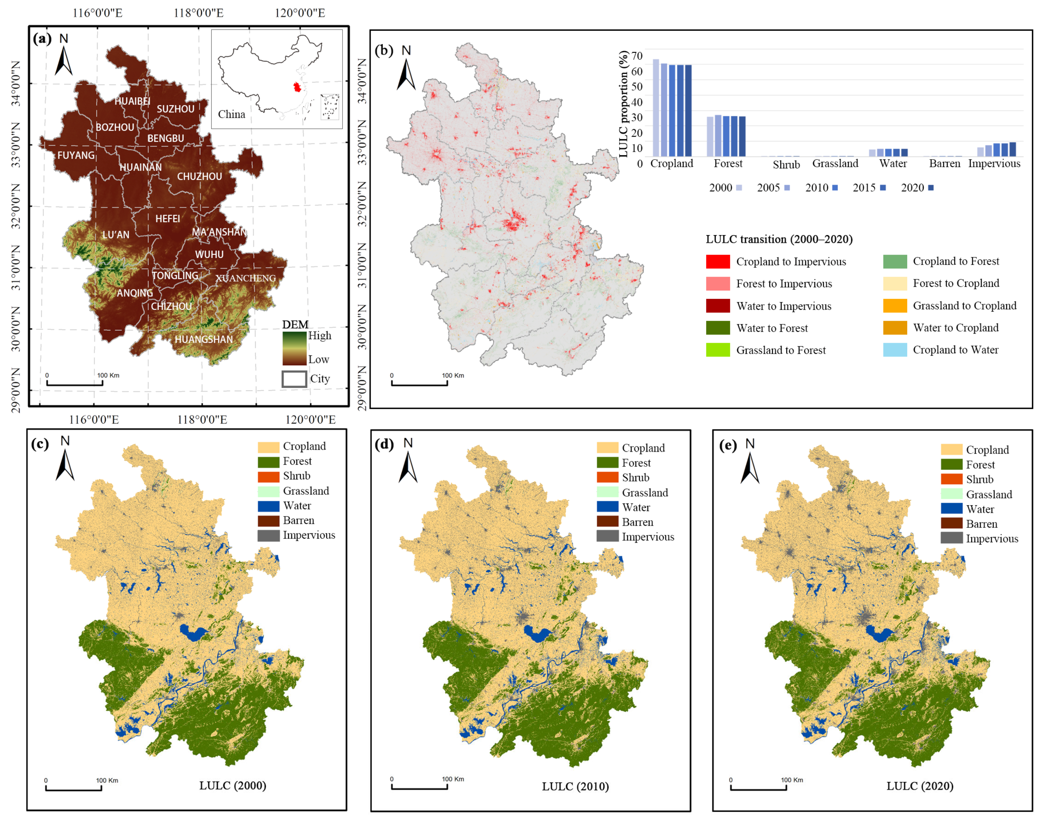
2.1. Study Area

Anhui Province, located in eastern China (latitude 29°41′ N to 34°38′ N, longitude 114°54′ E to a119°37′ E), spans approximately 140,000 km² and comprises 16 prefecture-level cities (Figure 1a). Situated along the middle to lower reaches of the Yangtze and Huai Rivers and at the core of the Yangtze River Delta, Anhui is characterized by diverse topography, including mountains, hills, plateaus, and plains. Its ecosystems cover forests, croplands, shrublands, grasslands, rivers, and lakes, creating a rich ecological mosaic. The climate transitions from temperate in the north to subtropical in the south result in significant regional variations in biodiversity and ecological resources.

Over the past two decades, Anhui Province has undergone rapid economic and urban transformation. The GDP surged from RMB 303.02 billion (USD 36.6 billion) in 2000 to RMB 3868.06 billion (USD 560.6 billion) in 2020, reflecting substantial economic growth, while the urbanization rate rose from 29.39% to 58.33% [26,27]. These developments have been accompanied by increasing population density, accelerated industrialization, and significant land use transformations. Croplands has historically dominated the northern regions, covering approximately 67% of Anhui Province’s total area. In contrast, urban land is primarily concentrated in the central and northern areas, accounts for about 9.5% of the province. Between 2000 and 2020, Anhui experienced substantial cropland losses and pronounced urban expansion in the central and northern areas (Figure 1b).

2.2. Data Source

This study utilized multi-source data to quantify the ESs. LULC was categorized into seven types: cropland, forest, shrub, grassland, impervious surfaces, barren land, and water bodies. All data in

Table 1. Summary of the primary data.

Data Type	Data Format	Data Source	Spatial Resolution
LULC	Raster	The 30 m annual land cover datasets and its dynamics in China from 1990 to 2021 [28]	30 m
Precipitation	Raster	National Earth System Science Data Center, National Science & Technology Infrastructure of China (http://www.geodata.cn, accessed on 17 January 2024).	1 km
Temperature	Raster	National Earth System Science Data Center, National Science & Technology Infrastructure of China (http://www.geodata.cn, accessed on 17 January 2024).	1 km
Evapotranspiration	Raster	National Earth System Science Data Center, National Science & Technology Infrastructure of China (http://www.geodata.cn, accessed on 17 January 2024).	1 km
Root depth, soil texture, and soil type	Raster	National Tibetan Plateau/Third Pole Environment Data Center (http://data.tpdc.ac.cn, accessed on 14 July 2023).	30 arc-second
Carbon density	Spreadsheet	China terrestrial ecosystem carbon density dataset [29]	/
Digital elevation model (DEM)	Raster	Geospatial Data Cloud (www.gscloud.cn, accessed on 12 July 2023).	90 m
Urbanization drivers	Spreadsheet	Anhui Provincial Bureau of Statistics (tjj.ah.gov.cn, accessed on 15 July 2023).	/

were resampled to a 30 m × 30 m grid scale to quantify ESs and urbanization drivers.

2.3. Quantification of ES Spatial-Temporal Distribution Characteristics

2.3.1. ESs Assessment

In this study, we selected five ESs based on the following criteria: (1) aligned with the ES categories defined in the Millennium Ecosystem Assessment [30]; (2) relevance to the natural environment, socioeconomic context, and ecological issues faced by the study area; and (3) data availability and reliability. The selected ESs were water conservation (WC), soil conservation (SC), habitat quality (HQ), carbon storage (CS), and water yield (WY) (

Table 2. Overview of ESs quantified in this study.

Category	Ecosystem Service	Abbreviation	Methodology
Regulating service	Water conservation	WC	Water balance equation
	Soil conservation	SC	Universal Soil Loss Equation
Supporting service	Habitat quality	HQ	InVEST model
	Carbon storage	CS	InVEST model
Provisioning service	Water yield	WY	InVEST model

). These ESs encompassed three main categories of ESs: regulating services, supporting services, and provisioning services [31]. We focused on five key regulating and provisioning ESs while excluding cultural services was primarily due to their strong relevance to LULC dynamics, which were the main pathways through which urbanization impacts ecosystems. Moreover, reliable and consistent data sources were available to parameterize the regulating services, supporting services and provisioning services. In contrast, cultural services are often intangible and difficult to measure spatially, making them less suitable for this type of large-scale spatial analysis.

Each ES was quantified at a 30 m × 30 m grid scale for the years 2000, 2005, 2010, 2015, and 2020. Detailed quantification methods and model parameters were provided in the Supplementary Materials. And the spatial distribution of these ESs was analyzed at the city scale using zonal statistics on the ArcGIS 10.7 platform. The study adopted the WGS_1984_UTM_Zone_50N coordinate projection to ensure data accuracy and consistency.

2.3.2. Geographically Weighted Regression

We used geographically weighted regression (GWR) to further explore the spatial interactions among ESs. The GWR model introduces a spatial weight matrix that allows regression coefficients to vary geographically based on the influence of nearby sampling points. This approach captures spatial non-stationarity and reveals the heterogeneous spatial effects of the independent variables on the dependent variable [32]. The mathematical expression for the GWR model is as follows:

$$y_i={\beta }_0\left({\mu }_i,{\nu }_i\right)+{\sum }_{k=1}^p {\beta }_k\left({\mu }_i,{\nu }_i\right)x_{ki}+{\epsilon }_i$$

(1)

where $y_i$ is the dependent variable at location $i$; $x_{ki}$ represents the $k$ independent variable at the $i$ location; ${\beta }_0\left({\mu }_i,{\nu }_i\right)$ is the intercept term that varies with spatial location $\left({\mu }_i,{\nu }_i\right)$; ${\beta }_k\left({\mu }_i,{\nu }_i\right)$ denotes the spatially varying coefficient for the $k$ independent variable; $\left({\mu }_i,{\nu }_i\right)$ refers to the geographic coordinates of location $i$; and ${\epsilon }_i$ is the error term. In this study, each ES was analyzed individually as a dependent variable in the GWR model to assess its spatial response across regions. A positive regression coefficient indicated a synergistic relationship, whereas a negative coefficient indicated a trade-off. Multicollinearity was not concerned in this analysis as only one dependent variable is used in each regression. We used Gaussian kernel to determine the weight and the Akaike Information Criterion corrected (AICc) to determine the bandwidth. The search range for the optimal bandwidth was set from 20 km to 150 km in 5 km increments.

2.4. Relationship Between Urbanization and ESs

2.4.1. Selection of Urbanization Drivers

We categorized urbanization into five dimensions: population urbanization, economic urbanization, spatial urbanization, ecological urbanization, and social urbanization according to the socio-economic context of the region [33]. Each dimension reflected specific characteristics and influences within the urbanization process. Specifically, population urbanization represented the concentration and migration of populations within cities and is a direct measure of urban growth [23]. Economic urbanization seized the trend of economic growth, optimized the industrial structure, and enhanced economic vitality [34]. Spatial urbanization reflected the expansion and intensification of urban spatial structure and land use. And ecological urbanization emphasized the balance between ecological protection and development [15]. Lastly, social urbanization highlighted the improvements in social welfare, public services, and residents’ quality of life during urbanization process [35].

To quantify these five dimensions, we selected 12 key urbanization drivers to assess the impact of various urbanization types on ESs (

Table 3. Urbanization category, urbanization drivers and abbreviations.

Category	Indicator	Abbreviation
Population Urbanization	Population Density (cap km−2)	pop
	Population Urbanization Rate (%)	ubr
Economic Urbanization	Per Capita GDP (104 RMB yr−1)	gdp
	Per Capita Disposable Income (RMB yr−1)	dpi
Spatial Urbanization	Urban Construction Proportion (%)	ucp
	Per Capita Urban Construction Area (m2 cap−1)	uca
Ecological Urbanization	Per Capita Park Green Area (ha cap−1)	pga
	Per Capita Industrial Wastewater Discharge (104 t cap−1)	iwd
Social Urbanization	Per Capita Grain Crop Yield (t cap−1)	gcy
	Per Capita Economic Crop (Oil) Yield (t cap−1)	ecy
	Civil Vehicle Ownership every 104 person (Vehicles 10−4 cap−1)	cvo
	People Participating in Medical Insurance proportion (%)	ppm

). The data sources are in Table 1. Indicator selection was guided by their representativeness in capturing urbanization processes and impacts on ESs, along with data availability. Data were collected from Anhui Provincial Bureau of Statistics. K-means clustering was employed to classify ESs and urbanization drivers, and the results were visualized in ArcGIS 10.7.

2.4.2. Hotspot Analysis of ES Levels and Urbanization Levels

To further analyze the spatial distribution characteristics of ES levels and urbanization levels, the average values of various urbanization drivers were used to represent urbanization levels. We used hotspot analysis to identify areas with high (hot spots) and low (cold spots) values in both ES and urbanization levels spatially. Hotspot analysis is based on the clustering nature of spatial data to help reveal patterns in spatial distribution. Points significantly higher than their surrounding areas are classified as hotspots, while those notably lower are identified as cold spots. This study used the Getis-Ord $G_i^{\ast }$ statistic to quantify the degree of spatial clustering. The calculation formula for the $G_i^{\ast }$ statistic is as follows [36]:

$$G_i^{\ast }={\displaystyle \frac{\sum _{j=1}^n{\omega }_{i,j}{x}_j-\overline{X}\sum _{j=1}^n{\omega }_{i,j}}{S\sqrt{\frac{\left[n\sum _{j=1}^n{\omega }_{i,j}^2-{\left(\sum _{j=1}^n{\omega }_{i,j}\right)}^2\right]}{n-1}}}}$$

(2)

where $G_i^{\ast }$ represents the spatial clustering statistic; $x_j$ is the attribute value of feature $j$; ${\omega }_{i,j}$ is the spatial weight between features $i$ and $j$; $n$ represents the total number of features; $\overline{X}$ and $S$ denote the mean and standard deviation of $x_j$, respectively. The Z-score is a standardized form of $G_i^{\ast }$ which determines the significance, a high positive Z-score indicates a statistically significant hotspot while a low negative Z-score indicates a significant coldspot. And the greater the absolute value of the Z-score, the stronger the clustering effect.

Through hotspot analysis, we identified and mapped the cold and hot spots for both ES levels and urbanization levels, displaying four distinct spatial patterns: (1) areas where both ES and urbanization levels are hotspots, (2) areas where both are cold spots, (3) areas where ES is a hotspot and urbanization levels is a cold spot, and (4) areas where ES is a cold spot and urbanization levels is a hotspot. This visualization effectively illustrated spatial homogeneity or heterogeneity between ES levels and urbanization levels, providing further insights of their spatial relationship.

2.4.3. Geographic Detector Model

To investigate the key urbanization drivers that impact on spatial heterogeneity of ESs, we utilized the geographic detector method to assess the explanatory power of potential urbanization drivers. The method is based on the principle of spatial stratified heterogeneity. Its core assumption is that if the independent variable significantly affects the dependent variable, the spatial distribution of the independent variable will be similar to the spatial distribution of the dependent variable [37]. In this study, ESs were treated as dependent variables and the urbanization drivers were served as independent variables. The $q$ value in the geographic detector measured the extent to which urbanization drivers explain the spatial heterogeneity of ecosystems and ranged between [0, 1]. A $q$ value closer to 1 indicated a stronger explanatory power of the independent variable for the dependent variable, while a lower $q$ value suggested a weaker explanatory power. The formula for calculating the $q$ value in the geographic detector is as follows [38]:

$$q=1-{\displaystyle \frac{\sum _{h=1}^L N_h{\sigma }_h^2}{N{\sigma }^2}}$$

(3)

where $h=1,\dots ,L$ represents the stratification of urbanization factors, which means classification or partitioning; $N_h$ and $N$ denote the number of units in stratum $h$ and in the entire region, respectively; ${\sigma }_h^2$ and ${\sigma }^2$ represent the variance within stratum $h$ and for the entire region, respectively.

Interaction detection within the geographic detector framework identifies the combined effects of different risk factors $X_s$ on the dependent variable. By analyzing these interactions, it is possible to determine whether the combined effect of these factors enhances or weakens the explanatory power of the dependent variable or whether the effect of each factor is independent. Detailed methods are shown in the Supplementary Materials (Table S7).

2.5. Identification of Relationships Among Urbanization, LULC, and ESs

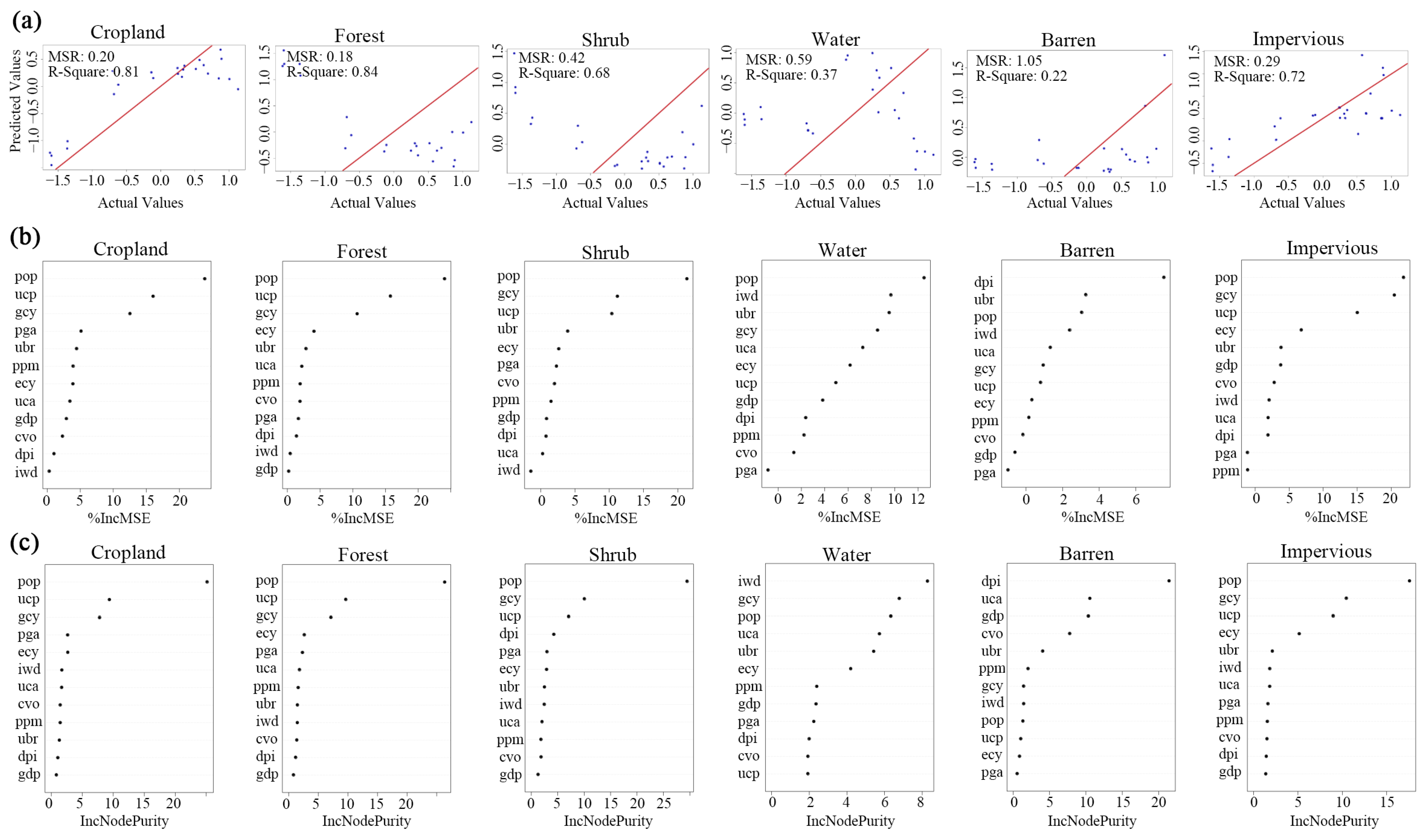
2.5.1. Random Forest Model

A random forest (RF) model was employed to analyze the relationships between urbanization drivers and LULC types, as well as the influences of LULC types on ESs. The RF model is an ensemble learning method based on decision trees which could capture complex and non-linear relationships [39]. It builds multiple decision trees during training and aggregates their predictions to improve accuracy and reduce overfitting.

The analysis used 12 urbanization drivers as predictors and seven LULC types as response variables to investigate how urbanization drive land use changes. Additionally, the relationships between LULC types and five ESs were examined by treating LULC types as predictors and each ES as the dependent variable. We gathered all data from 2000 to 2020 as a whole dataset. For the urbanization-LULC types analysis, the RF model was configured with 500 trees, and the number of variables randomly selected at each split was set to 4. The maximum tree depth was set to 20, and five-fold cross-validation was used to tune hyperparameters and reduce overfitting. For the LULC types-ES analysis, the model retained 500 trees, and the number of variables tried at each split was reduced to 2. Hyperparameter settings were validated using five-fold cross-validation. In both cases, 70% of the data was used to train the model and 30% was reserved for validation.

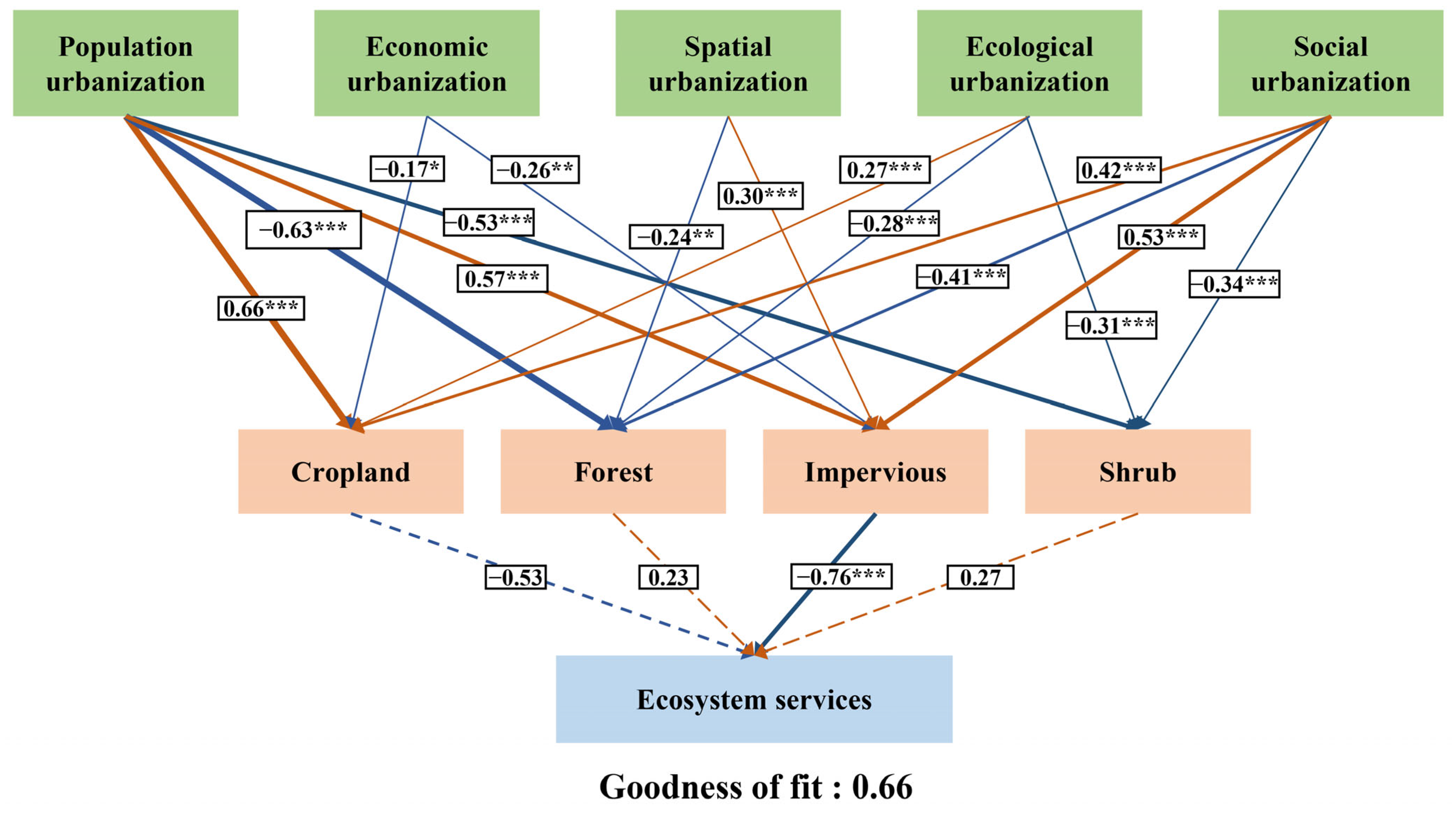
2.5.2. Partial Least Squares Path Modeling

We used Partial Least Squares Path Modeling (PLS-PM) to examine how urbanization influences ESs through LULC. This method is based on Partial Least Squares regression to analyze complex relationships between latent and observed variables [40]. In this study, the latent variables were the five dimensions of urbanization—population, economy, spatial, ecology, and society urbanization. And the observed variables were 12 corresponding urbanization drivers. Similarly, the latent variables for ES included five specific ESs: WC, SC, HQ, CS, and WY. The four LULC types with the most significant influence on ESs were served as mediating variables, as identified in the RF model results.

3. Results

3.1. Spatiotemporal Patterns and Characteristics of ESs and Urbanization

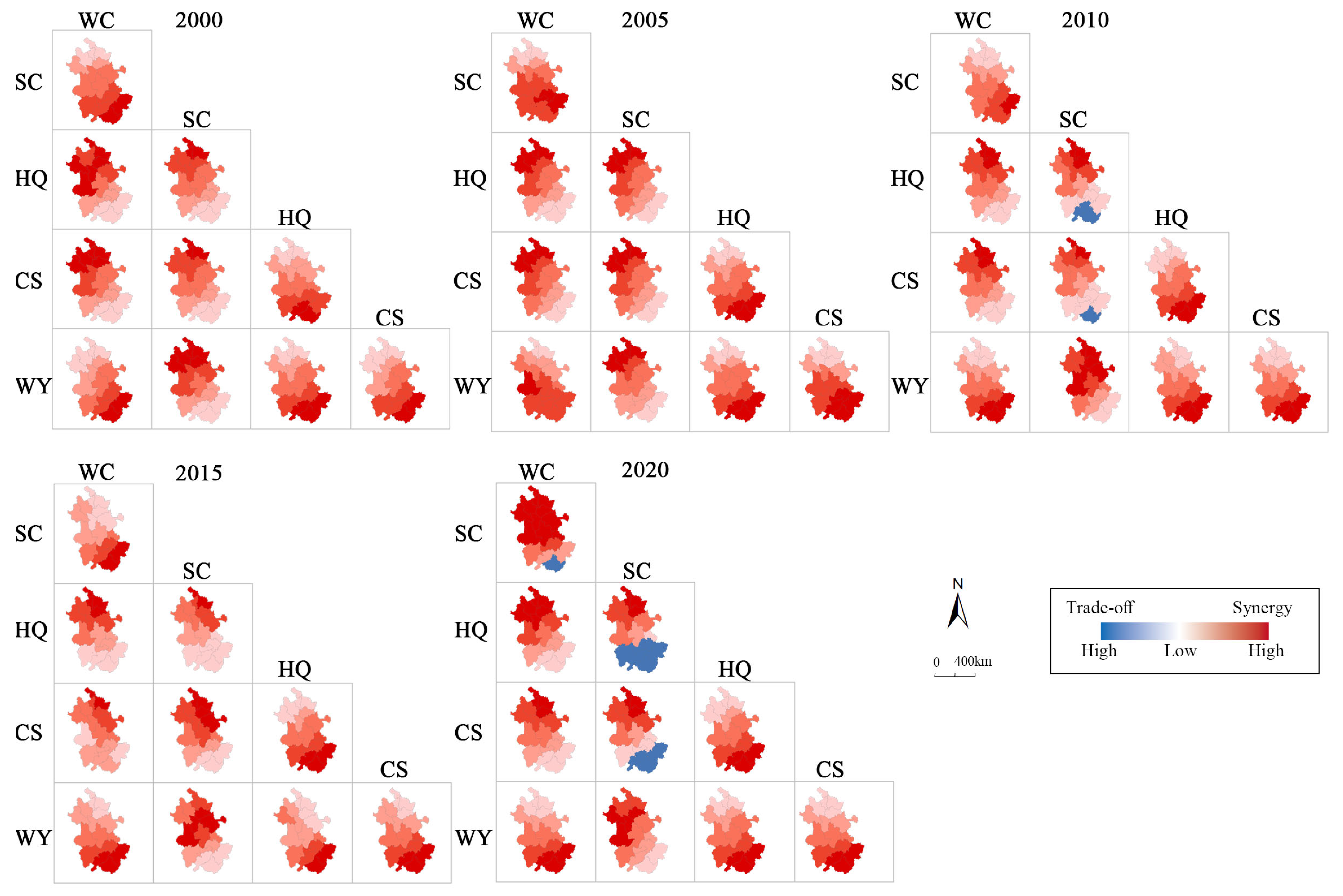
3.1.1. Spatiotemporal Variations and Trade-Offs of ESs

From 2000 to 2020, ESs in Anhui Province exhibited spatial heterogeneity in both spatial distribution and temporal variation (Figure 2a). Overall, various ESs, including WC, SC, HQ, CS, and WY, all displayed a spatial pattern with higher values in the southern mountainous and vegetated regions, and relatively lower values in the central and northern plain areas in Anhui Province.

In terms of temporal variation, each ES showed fluctuating trends over the 20 years period. WC, SC, and WY experienced a downward trend from 2000 to 2005 and then increased continually from 2005 to 2020. During this period, the maximum values of WC and WY rose from 978.08 mm and 1060.88 mm to 1159.92 mm and 1248.75 mm, respectively (Table S13). The highest value for SC increased from 1.47 t ha⁻¹ to 1.93 t ha⁻¹. After 2005, the variability among 16 cities of this three ESs became smaller (Figure 2b). In contrast, the value of HQ and CS increased from 2000 to 2005 and then decreased from 2005 to 2020. HQ value decreased from 0.0286 in 2005 to 0.0245 in 2020, and CS value decreased slightly every five years after reaching a peak of 8.92 Mg C ha⁻¹ in 2005. Moreover, the disparities of HQ and CS among 16 cities became larger during 2005 and 2020 (Figure 2b).

Spatially, all ESs increased gradually in the middle and southern areas, while unobvious value changes are observable in the northern regions. HQ and CS values remained high in the southern regions but showed limited change in the north.

The results of GWR showed there were trade-offs between HQ-SC, CS-SC in 2010 and 2020, and between SC-WC in 2020 in the southern areas in Anhui Province (Figure 3). These trade-offs might result from afforestation with monocultures that enhance SC, but the increased of a single land use type would reduce biodiversity and habitat complexity, thereby lowering the HQ.

The spatial extent of the synergistic regions between various ES pairs expanded throughout the study period, reflecting an overall increase in the spatial coherence of ES interactions. Strong synergies between pairs such as WC-SC, WC-WY, HQ-CS, HQ-WY, and CS-WY, which were particularly prominent in the southern areas. In contrast, synergies between ESs pairs like WC-HQ, WC-CS, SC-HQ, SC-CS, and SC-WY were most pronounced in central and northern areas where urban and agricultural land use predominate. The spatial heterogeneity of ES synergies can partly be attributed to land use differences. In the northern agricultural plains, the synergies among provisioning ESs were often stronger due to the homogeneous land use and standardized agricultural practices [41]. Meanwhile, southern hilly and forested areas with a more natural ecosystem and smaller anthropogenic disturbance often exhibited stronger synergies in regulating ESs [42].

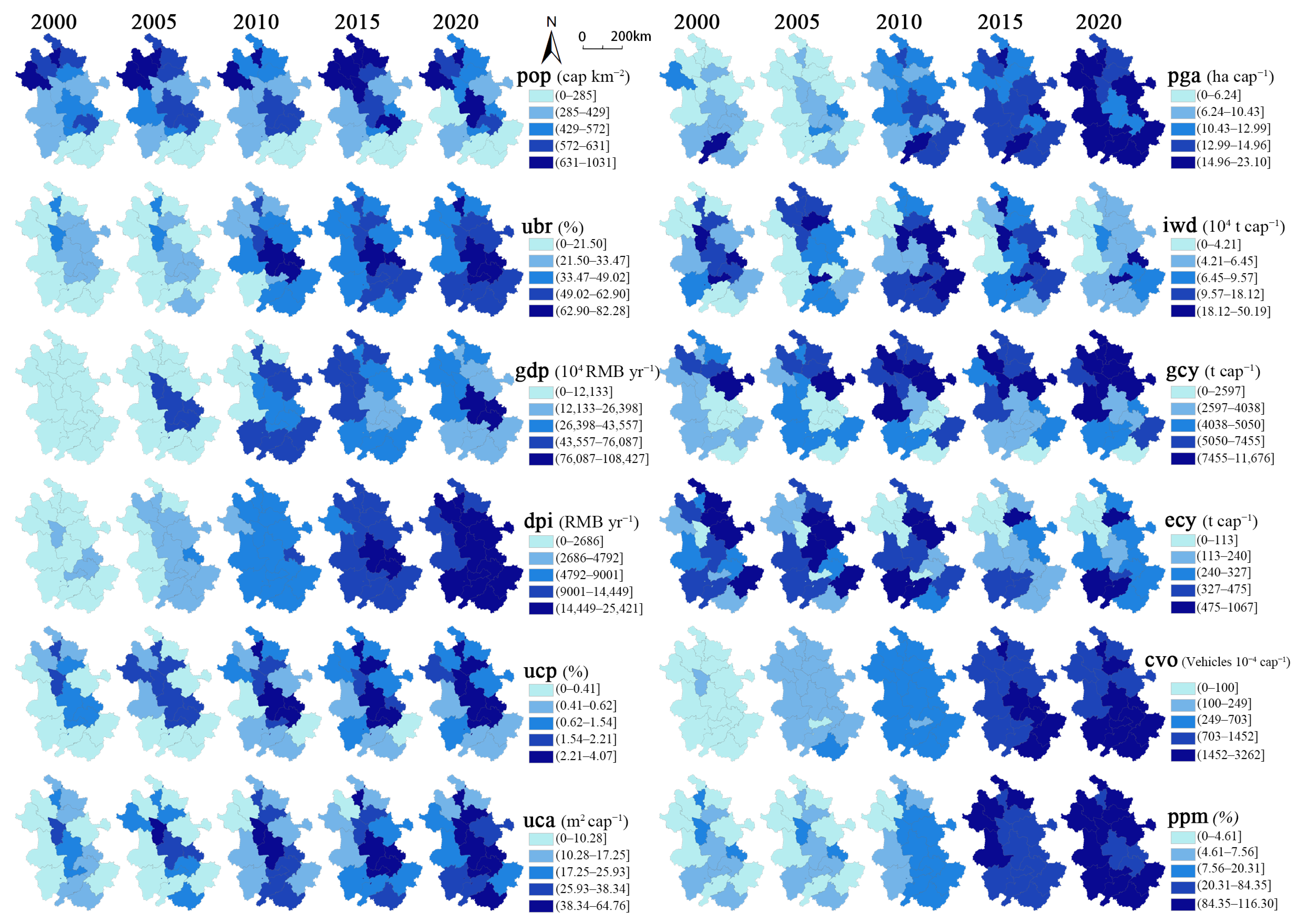
3.1.2. Spatiotemporal Variations of Urbanization Drivers

From 2000 to 2020, urbanization drivers in Anhui Province showed an overall upward trend. The spatial expansion moving from the central regions toward the north and east (Figure 4). During this period, population and economic urbanization such as pop, ubr, gdp, and dpi increased steadily particularly around central areas. This phenomenon illustrated the central regions were the core of population and economic urbanization. Drivers such as uca and ucp expanded from central areas to northern areas, reflecting the obvious spatial characteristics of urban construction expansion. In contrast, Iwd and ecy showed a decreasing trend indicating an increase in ecological pressure and crop yield pressure in Anhui Province. In addition, cvo and ppm growing rapidly from 2005 to 2020 which illustrated the social urbanization were prominent.

Overall, urbanization in Anhui Province over the past two decades has been characterized by intensified development in the central region and accelerated expansion toward the north. These changes have led to significant increases in economic output, population concentration, and urban land coverage.

3.2. Spatial Relationships Between Urbanization and ESs

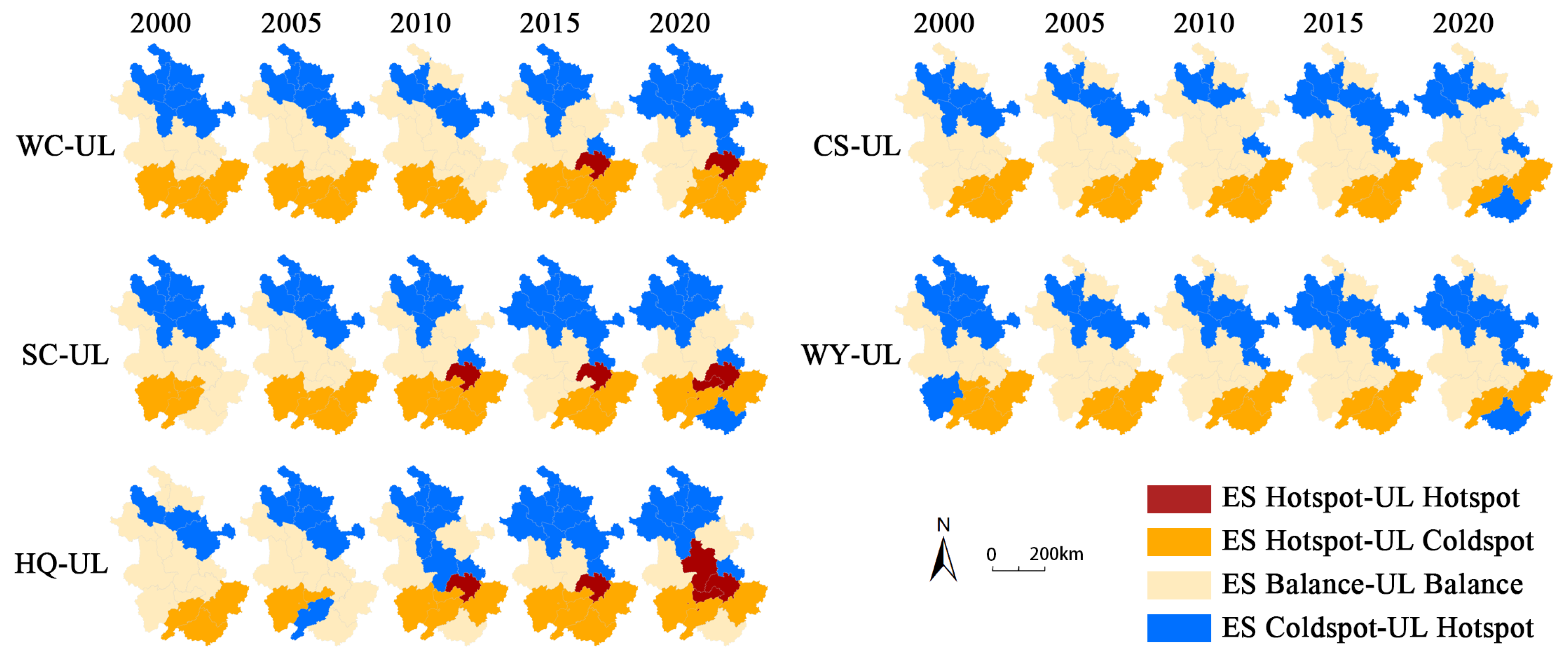
3.2.1. Spatial Distribution of Urbanization and ESs

The hotspot analysis results from 2000 to 2020 revealed marked spatial heterogeneity in the distribution of ESs and urbanization levels across Anhui Province (Figure 5). High ES levels were predominantly concentrated in the southern mountainous regions, where urbanization remained relatively low. This pattern was especially pronounced for WC, SC, and HQ, highlighting the substantial spatial disparities. In contrast, central Anhui exhibited a relatively balanced relationship between urbanization and ES provision. Overall, the spatial distributions of ES hotspots and urbanization levels displayed clear divergences, underscoring the need to further explore the underlying mechanisms driving these mismatches and to identify strategies for achieving a more sustainable balance between urban growth and ecosystem conservation.

3.2.2. Spatial Effects of Urbanization on ESs

The results of the geographic detector analysis revealed that different urbanization dimensions exhibited varied explanatory power for the spatial distribution of ESs (Figure 6). Among these dimensions, spatial urbanization and population urbanization had the greatest impact on the spatial changes of ESs, followed by social urbanization, while the impacts of ecological urbanization and economic urbanization are relatively weak. Among specific urbanization drivers, ucp demonstrated the highest explanatory power for the spatial distribution of HQ and CS. Pop had the most substantial influence on the spatial patterns of WC, SC, and WY. Additionally, ecy and gcy significantly contributed to the spatial differentiation of various ESs.

The interaction detector results indicated that the spatial impacts of urbanization drivers on ESs extended beyond the direct contributions of individual factors and were further amplified by their interactions. For example, with respect to WC, interactions between pop and ubr, ucp, uca, gcy, and ecy, as well as between ubr and ucp, exhibited two-factor enhancement effects on the spatial variation of WC (Tables S8–S12). Additionally, several interactions exhibited nonlinear enhancement effects, further underscoring the complexity of urbanization drivers in shaping the spatial distribution of ESs.

3.3. Linkages Among Urbanization, LULC, and ESs

3.3.1. Interconnections Between Urbanization and LULC

Moreover, we used RF model to explore how different types of urbanization influence ESs through LULC. The RF results revealed varying degrees of influence from urbanization drivers on different LULC types (Figure 7). Mean square residual (MSR) and R-square results (Figure 7a) demonstrated that the model performed best in predicting forest distribution, followed by cropland and impervious surfaces. This indicated that the RF model was able to capture the relationships between urbanization drivers and LULC types.

The variable importance analysis based on mean squared error (%IncMSE) (Figure 7b) highlighted the significant roles of specific urbanization drivers in influencing LULC types. For LULC types of croplands, forest, and impervious surface, pop, gcy, and ucp consistently emerged as the most influential factors. Additionally, ecy, ubr, and pga also showed substantial influence on the changes in these LULC types. The node purity (IncNodePurity) results (Figure 7c) further supported these findings. Due to the relatively small proportion of barren land and water bodies in Anhui Province, the RF model exhibited lower explanatory power for these LULC types. The limited spatial extent of these classes likely reduced the model’s sensitivity to urbanization drivers, resulting in weaker predictive performance.

Overall, these findings highlighted the complex interactions between urbanization drivers and LULC types and underscored the key role of urbanization drivers in shaping land use patterns.

3.3.2. Interconnections Between LULC and ESs

From 2000 to 2020, LULC in Anhui Province underwent significant changes (Figure 1). Cropland consistently accounted for the largest proportion which maintaining over 50% of the total area throughout the study period. And forest remained relatively stable at approximately 20%. In contrast, impervious surfaces increased significantly, from 6.2% in 2000 to 9.5% in 2020, reflecting the continued expansion of urban areas. We used RF model to further investigate the relationships between LULC and ESs. The results showed that the RF model had a good predictive power for HQ, CS and WC whose R-squares were 0.60, 0.41 and 0.40 (Figure 8a).

LULC types with higher %IncMSE and IncNodePurity values were identified as having stronger impacts on ES. The results identified shrubland, forest, and impervious surface as the most influential factors for HQ and CS, underscoring their critical role in supporting these ESs (Figure 8b,c). Meanwhile, water, forest, and impervious surface were identified as key drivers for WC. The replacement of natural and semi-natural landscapes with urban infrastructure reduced vegetation cover, increased surface runoff, and disrupted hydrological cycles.

3.3.3. Relationships Among Urbanization Types, LULC, and ESs

We employed the PLS-PM approach to further investigate the positive and negative relationships among different types of urbanization, LULC, and ESs (Figure 9). The results showed that population urbanization and social urbanization had strong significant positive effects on cropland and impervious surfaces, while significant negative impacts on forest and shrubland. This indicated that the expansion of urban population and improvement of social services tended to stimulate the demand for residential areas, infrastructure, and public amenities. The urban sprawl often occurred at the expense of natural land covers such as forests and shrubs. The population urbanization and social urbanization also needed to improve education, healthcare and public services, which accelerated the conversion of vegetated land into artificial surfaces. In addition, cropland was acted as a transitional or buffer land use in peri-urban areas. During the early stages of population urbanization and social urbanization, the croplands might be temporarily preserved or intensified for food production.

Furthermore, although different types of urbanization significantly influenced LULC types such as cropland, forest, and shrub, these LULC types did not exhibit significant direct effects on ESs in the PLS-PM results. This suggested that these LULC types may not serve as a strong mediating variable between urbanization and ES. Besides, impervious surface had a significant negative effect on ESs, indicating that the expansion of artificial land covers remains a critical driver of ecosystem degradation.

4. Discussion

4.1. Mechanisms of Urbanization Impacting ESs Through LULC Changes

This study revealed spatial and temporal variations in ESs across Anhui Province from 2000 to 2020, which had pronounced spatial heterogeneity and dynamic temporal trends. The higher levels of WC, SC, CS, HQ and WY in southern mountainous regions underscored the critical role of vegetation and land management in shaping ESs distributions [43,44]. In contrast, the northern and central plains exhibited lower ES values, reflecting the ecological stress associated with intensive land use and urban development.

The results also indicated that urbanization was a key driver for ESs changing while different dimensions of urbanization exerted varying effects. The spatial and population urbanization were identified as the most influential factors shaping the spatial distribution of ESs. This suggested that land consumption and population aggregation play central roles in either degrading or enhancing ecosystem functions [45]. These findings reflected the intensive land transformation and increased resource demands associated with dense urban growth.

Urbanization profoundly influenced ESs by driving extensive changes in LULC which acted as critical mediators linking urbanization processes to ES dynamics. From 2000 to 2020, Anhui Province underwent significant LULC transformations, characterized by the rapid expansion of impervious surfaces and changes in cropland and forest areas. These shifts were driven by various urbanization processes, including population growth, economic development, and spatial urbanization, which had both direct and indirect impacts on ES provision. Interestingly, cropland showed a dual role in shaping ES dynamics. On one hand, it supported provisioning services such as WY and SC, particularly in agriculturally intensive regions. On the other hand, economic urbanization drivers such as GDP and gross crop yield were associated with intensified agricultural practices that led to over-cultivation, soil erosion, and water scarcity, especially in the north. This illustrated a clear trade-off between food production and ecological sustainability, exacerbated by uneven urban–rural development strategies. Although LULC types such as cropland, forest and shrub exhibited explanatory power for ESs in the RF model, these variables did not show statistically significant direct paths to ESs in the PLS-PM analysis. This discrepancy likely caused by the fundamental differences between modeling approaches. The RF model excels at capturing nonlinear and interactive relationships and optimizing predictive accuracy, whereas PLS-PM focuses on estimating linear and direct relationships. In the presence of multicollinearity and overlapping influences among LULC, their individual contributions to ES might be diluted in the structural model, leading to non-significant paths despite their combined predictive importance. In other words, LULC types did not singly effect on ESs. Furthermore, the interaction detector analysis confirmed that many urbanization drivers do not act in isolation but interact in complex ways to shape ES patterns. These findings underscored the need for integrated urban development strategies that account for the compound and interactive effects of multiple drivers, rather than addressing each variable in isolation.

4.2. Implications and Recommendations

This study highlighted the critical role of land use and urbanization processes in shaping ESs. In the process of urbanization, growing populations and industrial activities generate substantial demand for water resources and ecological regulatory functions—demands that cannot be met solely by the local ecosystems within urbanized areas. Due to the hydrological connectivity of surface and groundwater systems, ecological resources originating in the southern mountainous regions play a vital role in sustaining both ecosystem functionality and economic activities across the province [46]. Thus, the development of central and northern Anhui inevitably relies on ecological contributions from the south. The spatial identification of ES hotspots and cold spots aligned with the policy direction of the European Green Deal, which promoted nature-positive urban development [47]. Our results provided actionable spatial insights that can support decision-makers in prioritizing areas for ecological protection, restoration, and green infrastructure investments. This reinforced the potential utility of ES mapping in balancing urban expansion with ecological integrity in line with emerging sustainability frameworks. Therefore, addressing how to alleviate the ecological pressure on southern regions while managing urbanized areas more sustainably has become a critical question for future planning.

Several implications for future environmental management and policy development emerged from the findings. First, given the significant spatial heterogeneity of ESs across Anhui Province and the observed synergy among different services, regional development should be approached through integrated planning, recognizing the ecological interdependence between regions [48]. The ESs provided by southern Anhui not only supported the resource demands of more urbanized areas but also contribute to the ecological and economic balance of the entire province. This mutual dependence called for a coordinated development strategy. Enhancing ecological compensation mechanisms can help promote conservation efforts in ecologically important areas, while also encourage sustainable practices in regions with high resource demand [49].

Second, the study revealed that spatial and population urbanization exert substantial pressure on ESs primarily through increased land demand and construction activity. This underscored the importance of sustainable land use planning to mitigate the ecological costs of urban expansion. Because multiple urbanization drivers interact synergistically to amplify ecological stress, policy interventions must address compound pressures rather than targeting individual drivers in isolation. For example, preserving and restoring forests and shrublands is essential for maintaining ES provision and buffering against the negative impacts of impervious surface growth. In agriculturally intensive areas, promoting sustainable farming techniques, such as crop diversification and water-efficient irrigation can help curb soil erosion, mitigate water stress, and reduce biodiversity loss, while maintaining agricultural productivity [50,51]. Furthermore, controlling population density and regulating urban sprawl can indirectly reduce land conversion pressure and preserve ecological functions. Our spatial prioritization results offered practical guidance for integrating ecosystem planning principles into land use policies. This included enhancing ecological connectivity through the design of continuous habitat corridors, and promoting multifunctionality by incorporating buffer zones that support biodiversity (e.g., pollination networks). Such integration would help embed ecological functionality into urban development plans, thereby aligning ecological protection with land management goals.

Lastly, since LULC change is the key pathway through which urbanization affects ESs, urbanization processes must be aligned with ecological objectives to ensure long-term sustainability [52,53]. Strategic interventions such as renewable resource utilization, mixed-use urban development, and adaptive land-use planning offer viable means to mitigate ecological degradation while sustaining economic growth. Specifically, solar panel installation and rooftop photovoltaics can be promoted through subsidies and smart-grid infrastructure [54]. Mixed-use urban development in cities can be implemented by revising zoning regulations to allow residential, commercial, and recreational functions within the same urban block [55]. For instance, high-density housing can be integrated with street-level markets, schools, and green spaces to reduce commuting distances and preserve ecological land at the periphery. Adaptive land use planning involves dynamically adjusting land use based on ecological sensitivity and urban growth trends [56]. In ecologically regions of southern Anhui, this could mean limiting the expansion of impervious surfaces and prioritizing ecological restoration, and in northern plains, guiding compact urban expansion onto previously degraded or low-productivity land. To enhance the practical relevance of our findings, the proposed policy strategies are aligned with existing international ecosystem management frameworks. For instance, advocating stronger protection and restoration of forests, wetlands, and shrublands directly supports the objectives of the EU Nature Restoration Act, which mandates the rehabilitation of degraded ecosystems to meet biodiversity and climate targets [57]. Moreover, the promotion of mixed-use green corridors and urban ecological buffers echoes the goals of Urban Greening Plans under the Covenant of Mayors, which encourage multifunctional land use to enhance climate resilience and urban livability [58]. By embedding our recommendations within these policy instruments, the study not only provided localized guidance for Anhui’s urban ecological planning, but also contributed to the growing body of ecosystem-based spatial strategies that are transferable across regions.

4.3. Limitations and Future Directions

This study had several limitations despite offering valuable insights. First, the findings are context-specific to Anhui Province and may not be directly generalizable to regions with different social–ecological conditions. Comparative studies across regions or countries are needed to validate and extend the conclusions. Additionally, the cultural ESs such as recreation and aesthetic appreciation were not included in this assessment due to difficulties in quantification and data availability at the regional scale. This exclusion may lead to an underestimation of the overall ES value particularly in areas where cultural ESs are prominent. Future studies should consider integrating cultural ESs to provide a more comprehensive assessment.

Second, although 30 m resolution data are appropriate for large-scale assessments, particularly at the provincial level, finer-resolution datasets (e.g., 10 m) could potentially improve the accuracy of ES estimates in urban areas with high land use heterogeneity. Future studies may benefit from integrating higher-resolution remote sensing data to capture more detailed spatial patterns. Besides, although the RF model exhibited relatively low R² values for grassland and barren land, this limitation did not substantially affect the overall conclusions. These land cover types constituted only a minor proportion of the total area in Anhui Province, and their contribution to ES supply was comparatively limited. Therefore, the low predictive accuracy in these categories had minimal influence on the spatial interpretation of ES patterns and urbanization impacts. Nonetheless, this finding highlighted the need for cautious interpretation of model outputs in regions where such LULC types are more prevalent. Otherwise, the biophysical parameters used in InVEST are often generalized or derived from literature, which may not fully reflect local ecological conditions. Sensitivity to these parameters might lead to variation in model outputs especially in areas with complex land use or topography [59]. And satellite-derived land cover maps could include classification errors, particularly in heterogeneous landscapes or rapidly changing urban zones. These uncertainties would affect the accuracy of ES quantification. Therefore, we suggested that decision-makers apply a precautionary approach in spatial planning and incorporate adaptive management strategies that allow for future updates and model refinements as higher-quality data become available.

Third, although this study explored the pathways linking urbanization and ESs through land use change, it did not fully incorporate the roles of policy, social behavior, or energy consumption patterns. These factors are increasingly relevant in shaping ecological outcomes. Future research should adopt more integrative frameworks that account for these factors to better understand the dynamics of coupled human–environment systems. This includes exploring feedback loops between ecological change and human responses, to better understand long-term socio-ecological dynamics [60].

5. Conclusions

By integrating spatial analysis, machine learning, and structural modeling, this study not only revealed the spatial distribution patterns of ESs but also elucidated the underlying mechanisms shaping these patterns. The results highlighted the critical roles of land use transitions as mediators and the combined impacts of different urbanization drivers. Based on these findings, there were three major conclusions: 1. ESs in Anhui Province displayed significant spatial and temporal heterogeneity at the urban scale, with synergistic relationships prevailing among different ESs. These patterns were closely linked to variations in land use types and ecological zones across cities. This underscored the need for differentiated planning and management strategies that are tailored to the specific ecological and land use conditions of each urban area. 2. Spatial and population urbanization exerted distinct yet interconnected influences on the spatial distribution of ESs. Spatial urbanization, characterized by built-up land expansion, led to the direct conversion and loss of ecological land. In contrast, population urbanization imposed indirect pressures by driving higher land demand and resource consumption. The geographic detector analysis further indicated that these urbanization factors interact synergistically, amplifying their combined impacts and underscoring the multifaceted nature of urbanization drivers. 3. LULC transitions served as critical pathways linking urbanization dynamics to changes in ESs supply. The expansion of construction land and the shrinkage of forest and cultivated land were key mediators through which urbanization reshaped ESs supply. This finding underscored the need for land use policies that integrate urban development with ecological sustainability goals. Based on the conclusions, this study proposes three implications to support more sustainable urban and ecological planning in the future. These findings are grounded in the specific socio-ecological context of Anhui Province. Therefore, caution should be exercised when applying the results to other regions without considering differences in environmental conditions, land use, and governance frameworks.

References

1. Costanza, R.; d’Arge, R.; de Groot, R.; Farber, S.; Grasso, M.; Hannon, B.; Limburg, K.; Naeem, S.; O’Neill, R.V.; Paruelo, J.; et al. The value of the world’s ecosystem services and natural capital. Nature 1997, 387, 253–260. [Google Scholar] [CrossRef]
2. Peng, J.; Wang, X.; Liu, Y.; Zhao, Y.; Xu, Z.; Zhao, M.; Qiu, S.; Wu, J. Urbanization impact on the supply-demand budget of ecosystem services: Decoupling analysis. Ecosyst. Serv. 2020, 44, 101139. [Google Scholar] [CrossRef]
3. Sun, L.; Chen, J.; Li, Q.; Huang, D. Dramatic uneven urbanization of large cities throughout the world in recent decades. Nat. Commun. 2020, 11, 5366. [Google Scholar] [CrossRef] [PubMed]
4. Field, C.B. Sharing the Garden. Science 2001, 294, 2490–2491. [Google Scholar] [CrossRef] [PubMed]
5. Bolund, P.; Hunhammar, S. Ecosystem services in urban areas. Ecol. Econ. 1999, 29, 293–301. [Google Scholar] [CrossRef]
6. McDonough, L.K.; Santos, I.R.; Andersen, M.S.; O’Carroll, D.M.; Rutlidge, H.; Meredith, K.; Oudone, P.; Bridgeman, J.; Gooddy, D.C.; Sorensen, J.P.R.; et al. Changes in global groundwater organic carbon driven by climate change and urbanization. Nat. Commun. 2020, 11, 1279. [Google Scholar] [CrossRef]
7. Xing, L.; Zhu, Y.; Wang, J. Spatial spillover effects of urbanization on ecosystem services value in Chinese cities. Ecol. Indic. 2021, 121, 107028. [Google Scholar] [CrossRef]
8. Maes, J.; Teller, A.; Erhard, M.; Liquete, C.; Braat, L.; Berry, P.; Egoh, B.; Puydarrieux, P.; Fiorina, C.; Santos, F. Mapping and Assessment of Ecosystems and their Services. In An Analytical Framework for Ecosystem Assessments Under Action; Publications Office of the European Union: Luxembourg, 2013; pp. 1–58. [Google Scholar]
9. Hermoso, V.; Carvalho, S.B.; Giakoumi, S.; Goldsborough, D.; Katsanevakis, S.; Leontiou, S.; Markantonatou, V.; Rumes, B.; Vogiatzakis, I.N.; Yates, K.L. The EU Biodiversity Strategy for 2030: Opportunities and challenges on the path towards biodiversity recovery. Environ. Sci. Policy 2022, 127, 263–271. [Google Scholar] [CrossRef]
10. De Marco, A.; Proietti, C.; Anav, A.; Ciancarella, L.; D’Elia, I.; Fares, S.; Fornasier, M.F.; Fusaro, L.; Gualtieri, M.; Manes, F.; et al. Impacts of air pollution on human and ecosystem health, and implications for the National Emission Ceilings Directive: Insights from Italy. Environ. Int. 2019, 125, 320–333. [Google Scholar] [CrossRef]
11. Nesbitt, L.; Meitner, M.J.; Sheppard, S.R.J.; Girling, C. The dimensions of urban green equity: A framework for analysis. Urban For. Urban Green. 2018, 34, 240–248. [Google Scholar] [CrossRef]
12. Boyce, J.K.; Zwickl, K.; Ash, M. Measuring environmental inequality. Ecol. Econ. 2016, 124, 114–123. [Google Scholar] [CrossRef]
13. Cowling, R.M.; Egoh, B.; Knight, A.T.; O’Farrell, P.J.; Reyers, B.; Rouget, M.; Roux, D.J.; Welz, A.; Wilhelm-Rechman, A. An operational model for mainstreaming ecosystem services for implementation. Proc. Natl. Acad. Sci. USA 2008, 105, 9483–9488. [Google Scholar] [CrossRef]
14. Thiery, W.; Lange, S.; Rogelj, J.; Schleussner, C.-F.; Gudmundsson, L.; Seneviratne, S.I.; Andrijevic, M.; Frieler, K.; Emanuel, K.; Geiger, T.; et al. Intergenerational inequities in exposure to climate extremes. Science 2021, 374, 158–160. [Google Scholar] [CrossRef] [PubMed]
15. Zhang, H.; Wang, Y.; Wang, C.; Yang, J.; Yang, S. Coupling analysis of environment and economy based on the changes of ecosystem service value. Ecol. Indic. 2022, 144, 109524. [Google Scholar] [CrossRef]
16. Wu, K.; Wang, D.; Lu, H.; Liu, G. Temporal and spatial heterogeneity of land use, urbanization, and ecosystem service value in China: A national-scale analysis. J. Clean. Prod. 2023, 418, 137911. [Google Scholar] [CrossRef]
17. Bi, Y.; Zheng, L.; Wang, Y.; Li, J.; Yang, H.; Zhang, B. Coupling relationship between urbanization and water-related ecosystem services in China’s Yangtze River economic Belt and its socio-ecological driving forces: A county-level perspective. Ecol. Indic. 2023, 146, 109871. [Google Scholar] [CrossRef]
18. Raudsepp-Hearne, C.; Peterson, G.D.; Bennett, E.M. Ecosystem service bundles for analyzing tradeoffs in diverse landscapes. Proc. Natl. Acad. Sci. USA 2010, 107, 5242–5247. [Google Scholar] [CrossRef]
19. Lemes de Oliveira, F.; Mahmoud, I. Desirable futures: Human-nature relationships in urban planning and design. Futures 2024, 163, 103444. [Google Scholar] [CrossRef]
20. de Groot, R.S.; Alkemade, R.; Braat, L.; Hein, L.; Willemen, L. Challenges in integrating the concept of ecosystem services and values in landscape planning, management and decision making. Ecol. Complex. 2010, 7, 260–272. [Google Scholar] [CrossRef]
21. Ouyang, X.; Tang, L.; Wei, X.; Li, Y. Spatial interaction between urbanization and ecosystem services in Chinese urban agglomerations. Land Use Policy 2021, 109, 105587. [Google Scholar] [CrossRef]
22. Ren, Q.; Liu, D.; Liu, Y. Spatio-temporal variation of ecosystem services and the response to urbanization: Evidence based on Shandong province of China. Ecol. Indic. 2023, 151, 110333. [Google Scholar] [CrossRef]
23. Li, Y.; Jia, L.; Wu, W.; Yan, J.; Liu, Y. Urbanization for rural sustainability—Rethinking China’s urbanization strategy. J. Clean. Prod. 2018, 178, 580–586. [Google Scholar] [CrossRef]
24. Zhao, F.; Yang, L.; Tang, J.; Fang, L.; Yu, X.; Li, M.; Chen, L. Urbanization–land-use interactions predict antibiotic contamination in soil across urban–rural gradients. Sci. Total Environ. 2023, 867, 161493. [Google Scholar] [CrossRef] [PubMed]
25. Yin, H.; Xiao, R.; Fei, X.; Zhang, Z.; Gao, Z.; Wan, Y.; Tan, W.; Jiang, X.; Cao, W.; Guo, Y. Analyzing “economy-society-environment” sustainability from the perspective of urban spatial structure: A case study of the Yangtze River delta urban agglomeration. Sustain. Cities Soc. 2023, 96, 104691. [Google Scholar] [CrossRef]
26. Anhui Provincial Bureau of Statistics. Anhui Statistical Yearbook 2001. Available online: http://tjj.ah.gov.cn (accessed on 14 July 2023).
27. Anhui Provincial Bureau of Statistics. Anhui Statistical Yearbook 2021. Available online: http://tjj.ah.gov.cn (accessed on 14 July 2023).
28. Yang, J.; Huang, X. The 30 m annual land cover dataset and its dynamics in China from 1990 to 2019. Earth Syst. Sci. Data 2021, 13, 3907–3925. [Google Scholar] [CrossRef]
29. Xu, L.; He, N.; Yu, G. A dataset of carbon density in Chinese terrestrial ecosystems (2010s). China Sci. Data 2019, 4, 90–91. [Google Scholar] [CrossRef]
30. Assessment, M.E. Millennium Ecosystem Assessment; Millennium Ecosystem Assessment: Washington, DC, USA, 2001; Volume 2. [Google Scholar]
31. Ouyang, Z.; Zheng, H.; Xiao, Y.; Polasky, S.; Liu, J.; Xu, W.; Wang, Q.; Zhang, L.; Xiao, Y.; Rao, E. Improvements in ecosystem services from investments in natural capital. Science 2016, 352, 1455–1459. [Google Scholar] [CrossRef]
32. Brunsdon, C.; Fotheringham, S.; Charlton, M. Geographically weighted regression. J. R. Stat. Soc. Ser. D 1998, 47, 431–443. [Google Scholar] [CrossRef]
33. Yu, B. Ecological effects of new-type urbanization in China. Renew. Sustain. Energy Rev. 2021, 135, 110239. [Google Scholar] [CrossRef]
34. Tian, Y.; Jiang, G.; Zhou, D.; Li, G. Systematically addressing the heterogeneity in the response of ecosystem services to agricultural modernization, industrialization and urbanization in the Qinghai-Tibetan Plateau from 2000 to 2018. J. Clean. Prod. 2021, 285, 125323. [Google Scholar] [CrossRef]
35. Liu, Y.; Li, Y. Revitalize the world’s countryside. Nature 2017, 548, 275–277. [Google Scholar] [CrossRef]
36. Getis, A.; Ord, J.K. The analysis of spatial association by use of distance statistics. Geogr. Anal. 1992, 24, 189–206. [Google Scholar] [CrossRef]
37. Wang, J.; Xu, C. Geodetector: Principle and prospective. Acta Geogr. Sin. 2017, 72, 116–134. Available online: http://www.geog.com.cn/CN/10.11821/dlxb201701010 (accessed on 20 July 2024). (In Chinese with English abstract).
38. Gu, C. Urbanization: Positive and negative effects. Sci. Bull. 2019, 64, 281–283. [Google Scholar] [CrossRef]
39. Schoppa, L.; Disse, M.; Bachmair, S. Evaluating the performance of random forest for large-scale flood discharge simulation. J. Hydrol. 2020, 590, 125531. [Google Scholar] [CrossRef]
40. Zhao, Y.-q.; Shen, J.; Feng, J.-m.; Wang, X.-z. Relative contributions of different sources to DOM in Erhai Lake as revealed by PLS-PM. Chemosphere 2022, 299, 134377. [Google Scholar] [CrossRef] [PubMed]
41. Rodríguez, J.P.; Beard, T.D., Jr.; Bennett, E.M.; Cumming, G.S.; Cork, S.J.; Agard, J.; Dobson, A.P.; Peterson, G.D. Trade-offs across space, time, and ecosystem services. Ecol. Soc. 2006, 11, 28. [Google Scholar] [CrossRef]
42. Du, X.; Jian, J.; Du, C.; Stewart, R.D. Conservation management decreases surface runoff and soil erosion. Int. Soil Water Conserv. Res. 2022, 10, 188–196. [Google Scholar] [CrossRef]
43. Mouchet, M.; Paracchini, M.-L.; Schulp, C.; Stürck, J.; Verkerk, P.; Verburg, P.; Lavorel, S. Bundles of ecosystem (dis) services and multifunctionality across European landscapes. Ecol. Indic. 2017, 73, 23–28. [Google Scholar] [CrossRef]
44. Tong, X.; Brandt, M.; Yue, Y.; Ciais, P.; Rudbeck Jepsen, M.; Penuelas, J.; Wigneron, J.-P.; Xiao, X.; Song, X.-P.; Horion, S. Forest management in southern China generates short term extensive carbon sequestration. Nat. Commun. 2020, 11, 129. [Google Scholar] [CrossRef]
45. Bennett, E.M.; Peterson, G.D.; Gordon, L.J. Understanding relationships among multiple ecosystem services. Ecol. Lett. 2009, 12, 1394–1404. [Google Scholar] [CrossRef] [PubMed]
46. Deng, C.; Liu, J.; Liu, Y.; Li, Z.; Nie, X.; Hu, X.; Wang, L.; Zhang, Y.; Zhang, G.; Zhu, D.; et al. Spatiotemporal dislocation of urbanization and ecological construction increased the ecosystem service supply and demand imbalance. J. Environ. Manag. 2021, 288, 112478. [Google Scholar] [CrossRef] [PubMed]
47. Fetting, C. The European Green Deal; ESDN Report; The ESDN Office: Vienna, Austria, 2020; Volume 2, 53p, Available online: https://www.sd-network.eu/?k=sdg,green+deal (accessed on 20 June 2024).
48. Schneider, F.; Kallis, G.; Martinez-Alier, J. Crisis or opportunity? Economic degrowth for social equity and ecological sustainability. Introduction to this special issue. J. Clean. Prod. 2010, 18, 511–518. [Google Scholar] [CrossRef]
49. Yu, B.; Xu, L. Review of ecological compensation in hydropower development. Renew. Sustain. Energy Rev. 2016, 55, 729–738. [Google Scholar] [CrossRef]
50. Wang, S.; Bai, X.; Zhang, X.; Reis, S.; Chen, D.; Xu, J.; Gu, B. Urbanization can benefit agricultural production with large-scale farming in China. Nat. Food 2021, 2, 183–191. [Google Scholar] [CrossRef] [PubMed]
51. Santos, M.M.; Lanzinha, J.C.G.; Ferreira, A.V. Review on urbanism and climate change. Cities 2021, 114, 103176. [Google Scholar] [CrossRef]
52. Butler, C.D.; Oluoch-Kosura, W. Linking Future Ecosystem Services and Future Human Well-being. Ecol. Soc. 2006, 11, 30. Available online: https://www.ecologyandsociety.org/vol11/iss1/art30/ (accessed on 20 June 2024). [CrossRef]
53. Tu, K.-J.; Lin, L.-T. Evaluative structure of perceived residential environment quality in high-density and mixed-use urban settings: An exploratory study on Taipei City. Landsc. Urban Plan. 2008, 87, 157–171. [Google Scholar] [CrossRef]
54. Brown, M.A.; Zhou, S. Smart-grid policies: An international review. In Advances in Energy Systems: The Large-Scale Renewable Energy Integration Challenge; John Wiley & Sons: Hoboken, NJ, USA, 2019; pp. 127–147. [Google Scholar] [CrossRef]
55. Kausar, A.; Zubair, S.; Sohail, H.; Anwar, M.M.; Aziz, A.; Vambol, S.; Vambol, V.; Khan, N.A.; Poteriaiko, S.; Tyshchenko, V. Evaluating the challenges and impacts of mixed-use neighborhoods on urban planning: An empirical study of a megacity, Karachi, Pakistan. Discov. Sustain. 2024, 5, 24. [Google Scholar] [CrossRef]
56. Li, L.; Huang, X.; Wu, D.; Yang, H. Construction of ecological security pattern adapting to future land use change in Pearl River Delta, China. Appl. Geogr. 2023, 154, 102946. [Google Scholar] [CrossRef]
57. Cliquet, A.; Aragão, A.; Meertens, M.; Schoukens, H.; Decleer, K. The negotiation process of the EU Nature Restoration Law Proposal: Bringing nature back in Europe against the backdrop of political turmoil? Restor. Ecol. 2024, 32, e14158. [Google Scholar] [CrossRef]
58. Basso, M.; Tonin, S. The implementation of the Covenant of Mayors initiative in European cities: A policy perspective. Sustain. Cities Soc. 2022, 78, 103596. [Google Scholar] [CrossRef]
59. Mukhopadhyay, A.; Hati, J.P.; Acharyya, R.; Pal, I.; Tuladhar, N.; Habel, M. Global trends in using the InVEST model suite and related research: A systematic review. Ecohydrol. Hydrobiol. 2025, 25, 389–405. [Google Scholar] [CrossRef]
60. Hastik, R.; Basso, S.; Geitner, C.; Haida, C.; Poljanec, A.; Portaccio, A.; Vrščaj, B.; Walzer, C. Renewable energies and ecosystem service impacts. Renew. Sustain. Energy Rev. 2015, 48, 608–623. [Google Scholar] [CrossRef]
61. Fu, B. On the calculation of the evaporation from land surface. Sci. Atmos. Sin. 1981, 5, 23–29. [Google Scholar]
62. Zhang, L.; Hickel, K.; Dawes, W.R.; Chiew, F.H.S.; Western, A.W.; Briggs, P.R. A rational function approach for estimating mean annual evapotranspiration. Water Resour. Res. 2004, 40. [Google Scholar] [CrossRef]
63. Zhao, J.; Yang, Z.; Govers, G. Soil and water conservation measures reduce soil and water losses in China but not down to background levels: Evidence from erosion plot data. Geoderma 2019, 337, 729–741. [Google Scholar] [CrossRef]
64. Wischmeier, W.H.; Smith, D.D. Predicting Rainfall Erosion Losses: A Guide to Conservation Planning. Department of Agriculture, Science and Education Administration. 1978. 67p. Available online: https://www.researchgate.net/profile/Heriansyah-Putra-2/post/Which-formula-is-correct/attachment/59d64d4e79197b80779a6e2c/AS%3A487650378424321%401493276318482/download/USLE.pdf (accessed on 5 June 2025).
65. Williams, J.; Jones, C.; Dyke, P. The EPIC model and its application. In Proceedings of the ICRISAT-IBSNAT-SYSS Symp. on Minimum Data Sets for Agrotechnology Transfer. ICRISAT-IBSNAT, Patancheru, India, 21–26 March 1984; pp. 111–121. [Google Scholar]
66. Desmet, P.J.; Govers, G. A GIS procedure for automatically calculating the USLE LS factor on topographically complex landscape units. J. Soil Water Conserv. 1996, 51, 427–433. [Google Scholar] [CrossRef]
67. Oliveira, A.H.; da Silva, M.A.; Silva, M.L.N.; Curi, N.; Neto, G.K.; de Freitas, D.A.F. Development of topographic factor modeling for application in soil erosion models. In Soil Processes and Current Trends in Quality Assessment; Soriano, M.C.H., Ed.; InTech: Rijeka, Croatia, 2013; Volume 4, pp. 111–138. [Google Scholar] [CrossRef]
68. Nelson, E.; Polasky, S.; Lewis, D.J.; Plantinga, A.J.; Lonsdorf, E.; White, D.; Bael, D.; Lawler, J.J. Efficiency of incentives to jointly increase carbon sequestration and species conservation on a landscape. Proc. Natl. Acad. Sci. USA 2008, 105, 9471–9476. [Google Scholar] [CrossRef]
69. Stanford University; U.o.M.; Chinese Academy of Sciences; The Nature Conservancy; World Wildlife Fund; Stockholm Resilience Centre and the Royal Swedish Academy of Sciences. Natural Capital Project. InVEST 0.0 2024. Available online: https://naturalcapitalproject.stanford.edu/software/invest (accessed on 20 June 2024).
70. Cao, Y.; Wang, C.; Su, Y.; Duan, H.; Wu, X.; Lu, R.; Su, Q.; Wu, Y.; Chu, Z. Study on Spatiotemporal Evolution and Driving Forces of Habitat Quality in the Basin along the Yangtze River in Anhui Province Based on InVEST Model. Land 2023, 12, 1092. [Google Scholar] [CrossRef]
71. Xia, H.; Yuan, S.; Prishchepov, A.V. Spatial-temporal heterogeneity of ecosystem service interactions and their social-ecological drivers: Implications for spatial planning and management. Resour. Conserv. Recycling 2023, 189, 106767. [Google Scholar] [CrossRef]
72. Zhang, G.; Quan, L. Impact of Habitat Quality Changes on Regional Thermal Environment: A Case Study in Anhui Province, China. Sustainability 2024, 16, 8560. [Google Scholar] [CrossRef]
Figure 1. Study area. (a) Location, elevation and prefecture-level cities; (b) LULC transition from 2000−2020, and the proportion trend of LULC; (c) LULC in 2000; (d) LULC in 2010; (e) LULC in 2020.
Land 14 01238 g001
Figure 2. ESs dynamics. (a) the spatiotemporal pattern of ESs; (b) annual value trend of each ES.
Land 14 01238 g002
Figure 3. Spatiotemporal synergies and trade-offs of ESs pairs in 2000, 2005, 2010, 2015, and 2020.
Land 14 01238 g003
Figure 4. The spatiotemporal patterns of urbanization drivers.
Land 14 01238 g004
Figure 5. Spatiotemporal distribution of hot spots and cold spots changes in ES levels and urbanization levels (UL) in 2000–2020. Note: no areas exhibit ES cold spots–UL cold spots.
Land 14 01238 g005
Figure 6. Explanatory power of urbanization drivers on ESs (q value).
Land 14 01238 g006
Figure 7. Relationship between urbanization drivers and LULC types. (a) Model performance for each LULC type based on mean square residual (MSR) and R-squared; (b) variable importance based on mean squared error (%IncMSE); (c) variable importance based on node purity (IncNodePurity). Note: grassland-urbanization demonstrated a very low R-square value, but it is not presented here.
Land 14 01238 g007
Figure 8. Relationship between LULC types and ESs. (a) Model performance for each ES based on mean square residual (MSR) and R-squared; (b) variable importance based on mean squared error (%IncMSE); (c) variable importance based on node purity (IncNodePurity).
Land 14 01238 g008
Figure 9. This figure illustrates the structural relationships among urbanization types, LULC, and ESs based on the PLS-PM. Note: The width of the arrows represents the magnitude of the standardized path coefficients: thicker lines indicate stronger effects, while thinner lines denote weaker relationships. Blue arrows represent negative correlations, and orange arrows indicate positive correlations. Asterisks denote significance levels (*** p < 0.001, ** p < 0.01, * p < 0.05). Solid lines represent statistically significant relationships (p < 0.05) and dashed lines denote non-significant paths.
Land 14 01238 g009