


A BiLSTM-Based Hybrid Ensemble Approach for Forecasting Suspended Sediment Concentrations: Application to the Upper Yellow River

Abstract
1. Introduction
2. Methods
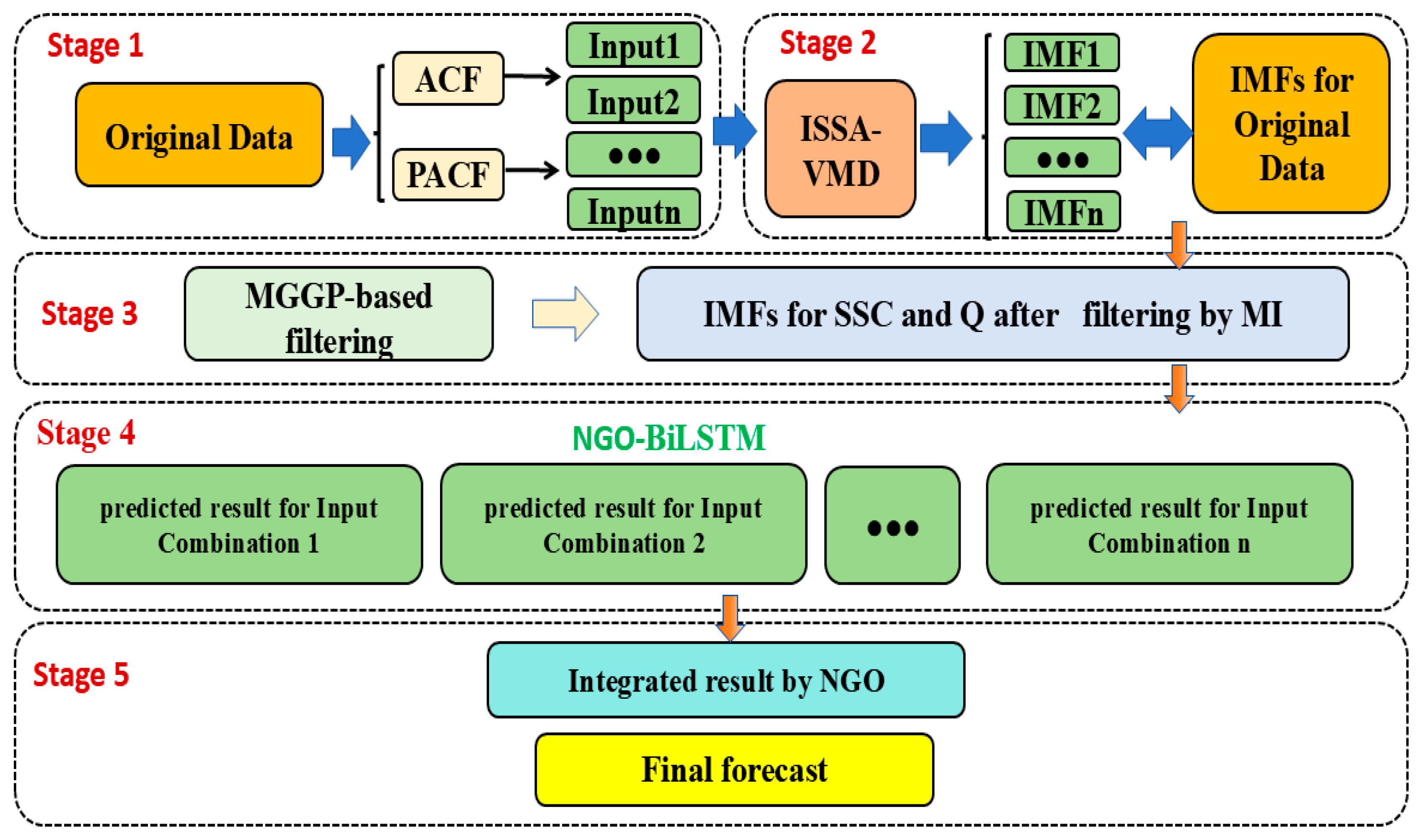
2.1. The Proposed Ensemble Model
2.2. Variational Mode Decomposition(VMD)
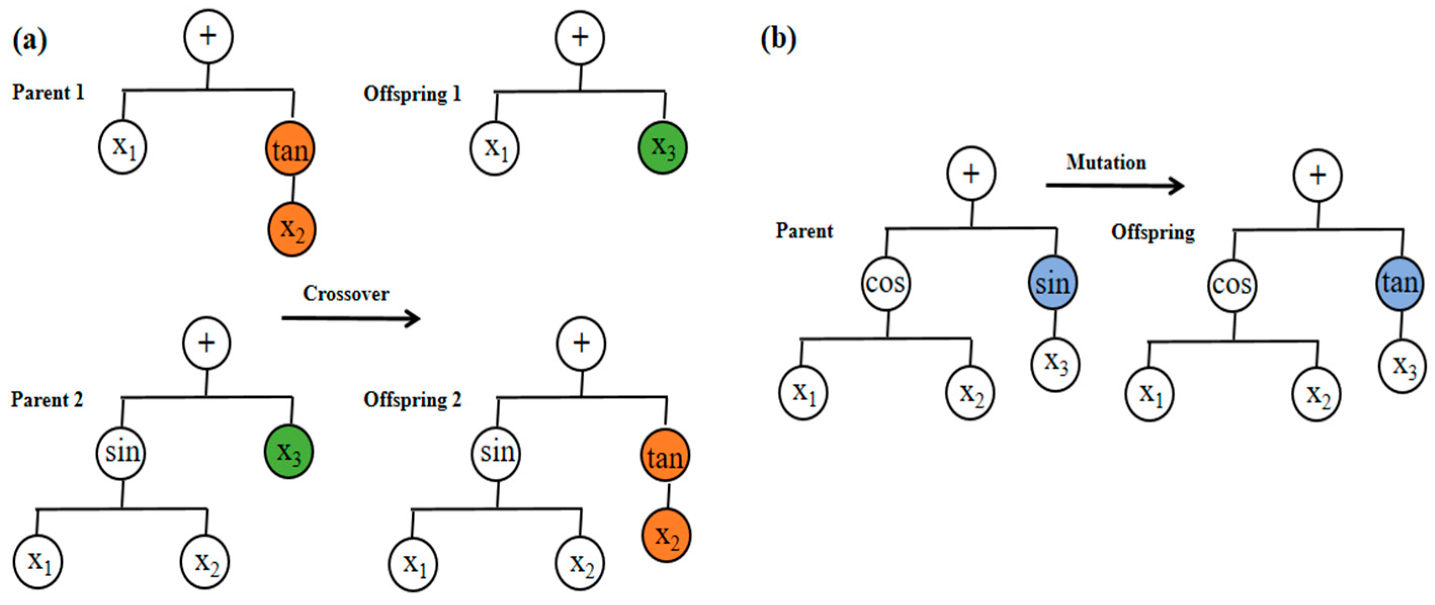
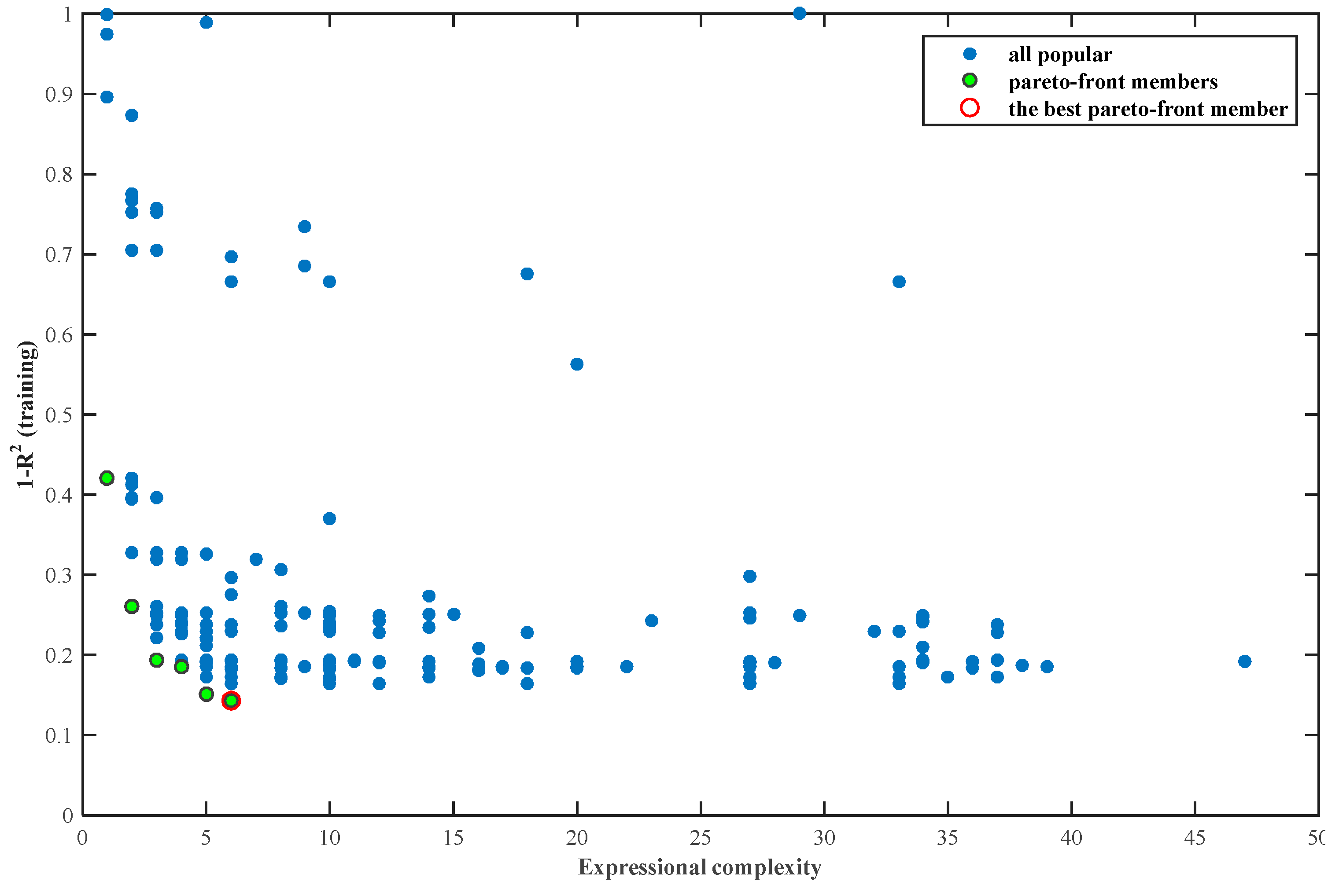
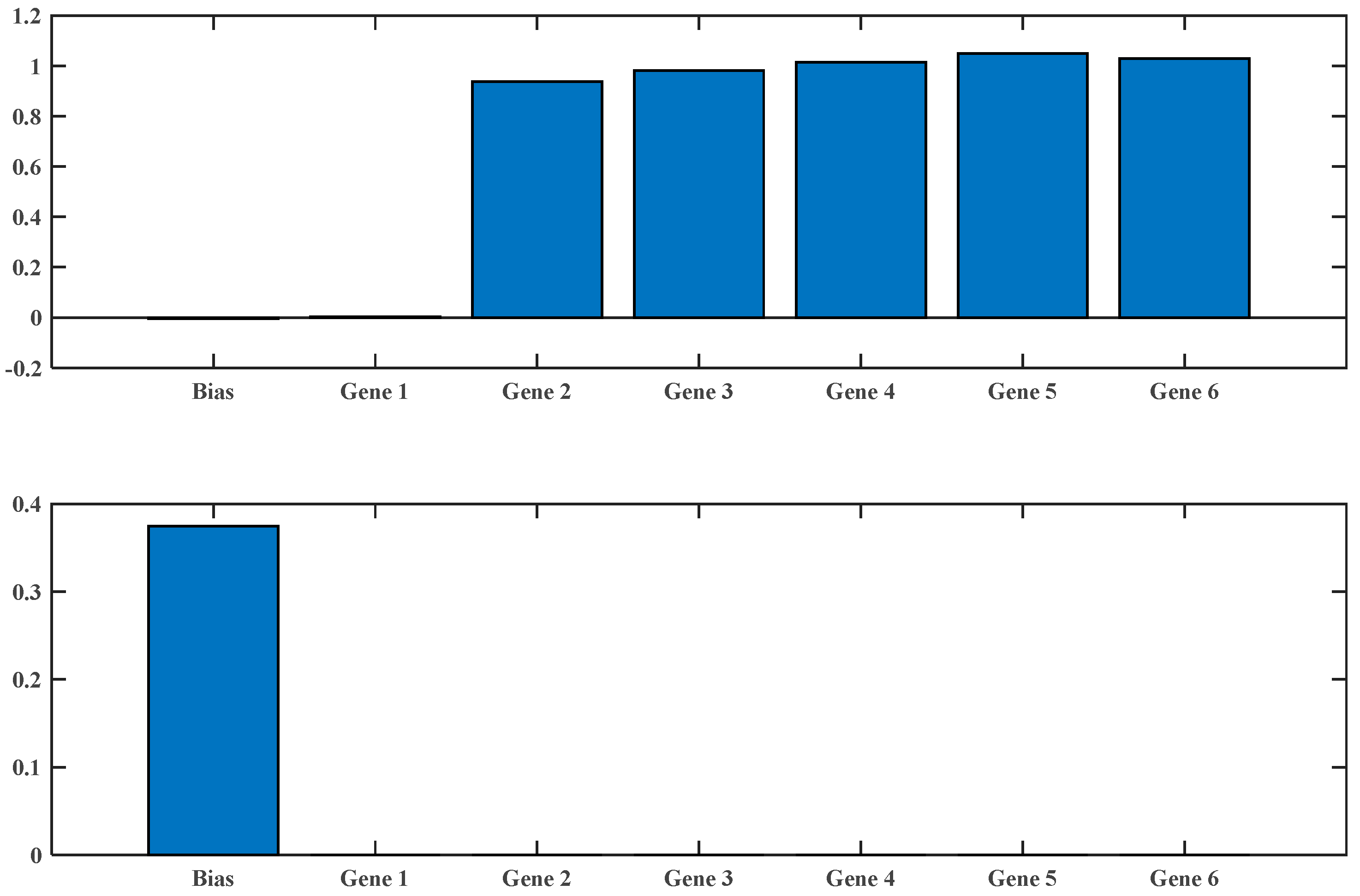
2.3. Multi-Gene Genetic Programming (MGGP)
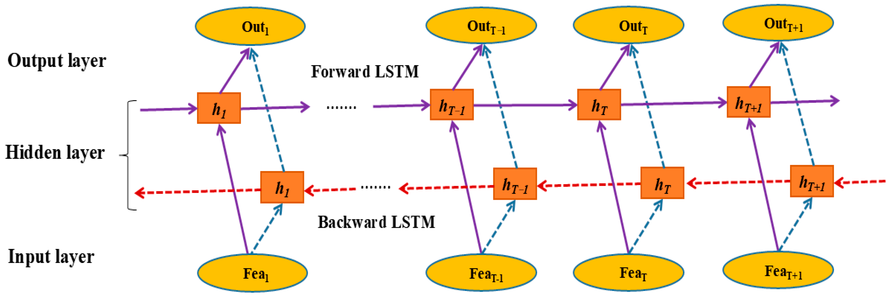
2.4. Bidirectional Long Short-Term Memory (BILSTM)
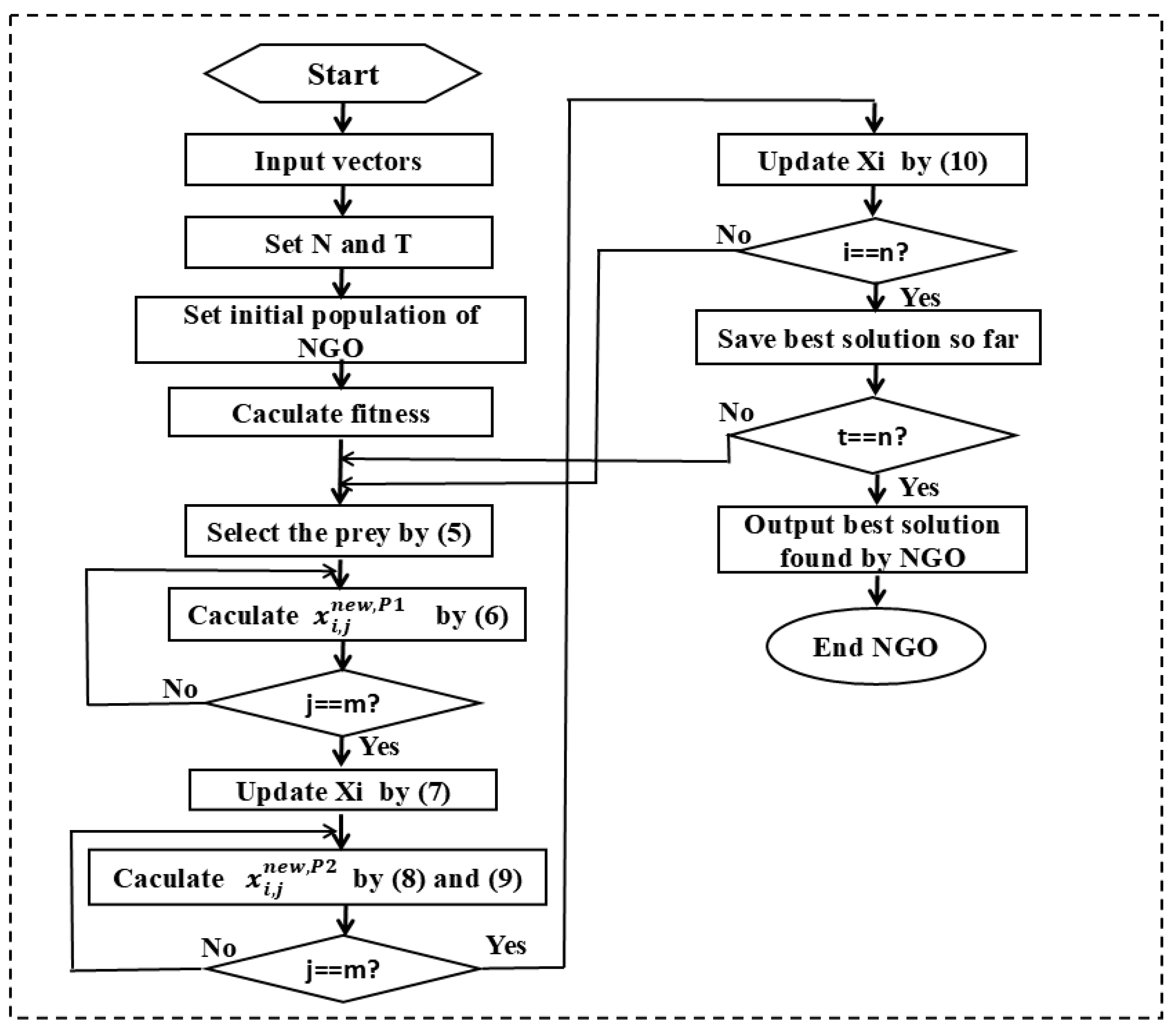
2.5. Northern Goshawk Optimization(NGO)
2.6. Performance Evaluation Criteria
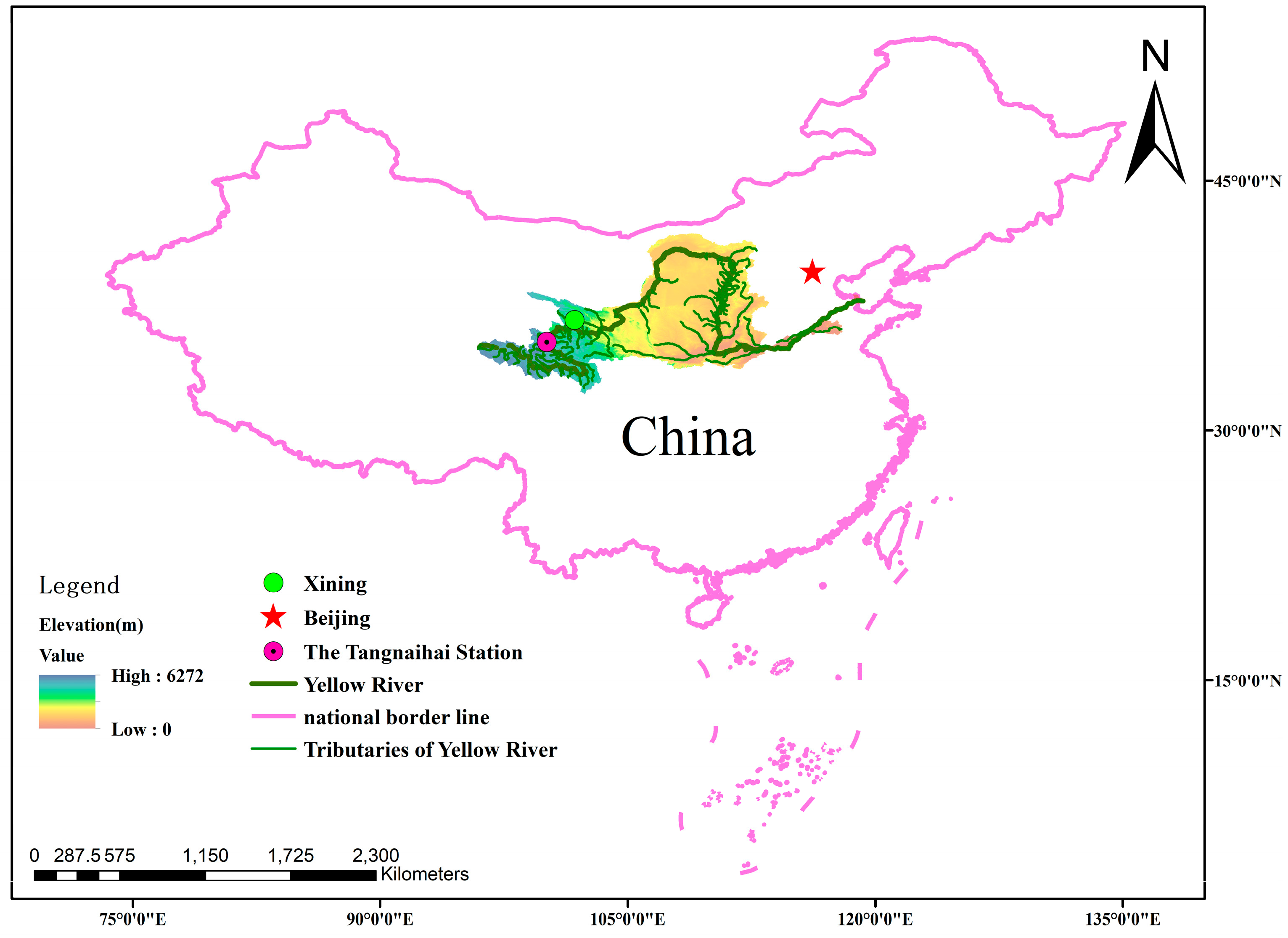
3. Research Area
4. Results
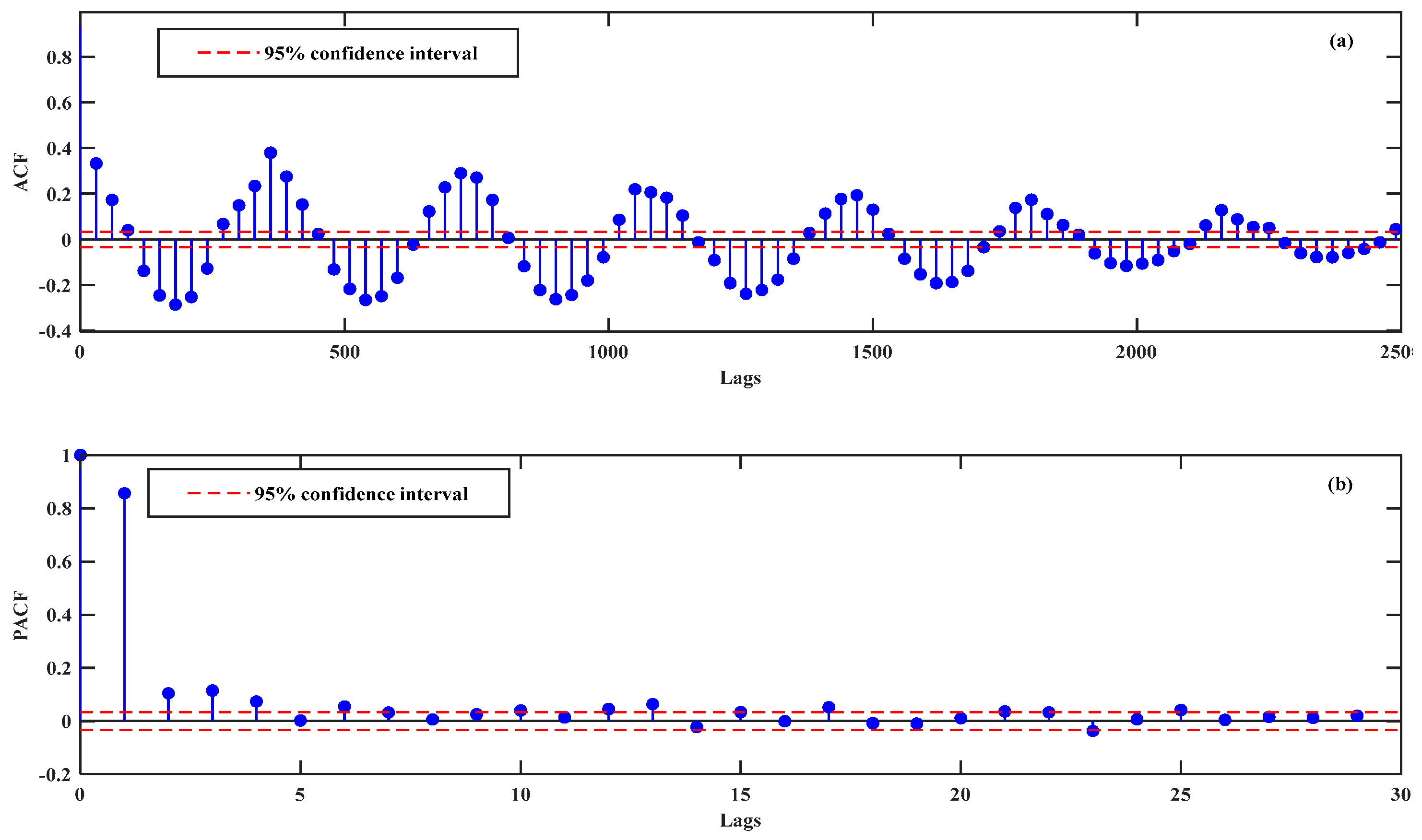
4.1. Selection of Input Vector
4.2. Data Decomposition and Filtering
4.3. Model Optimization and Performance Evaluation
4.3.1. Hyperparameter Optimization of BiLSTM Using NGO
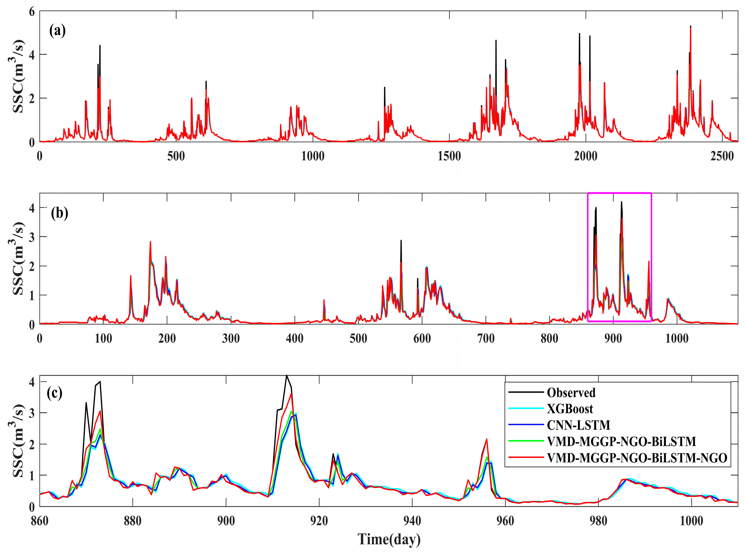
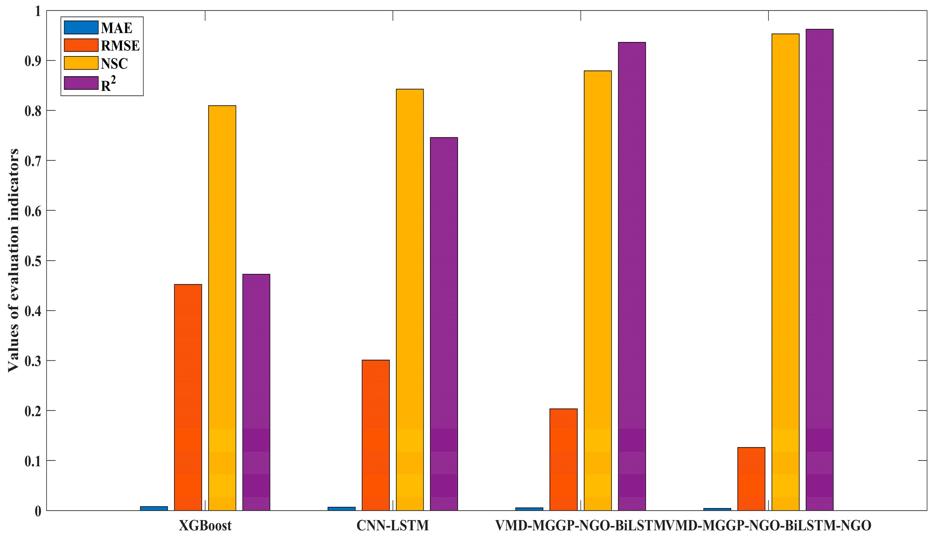
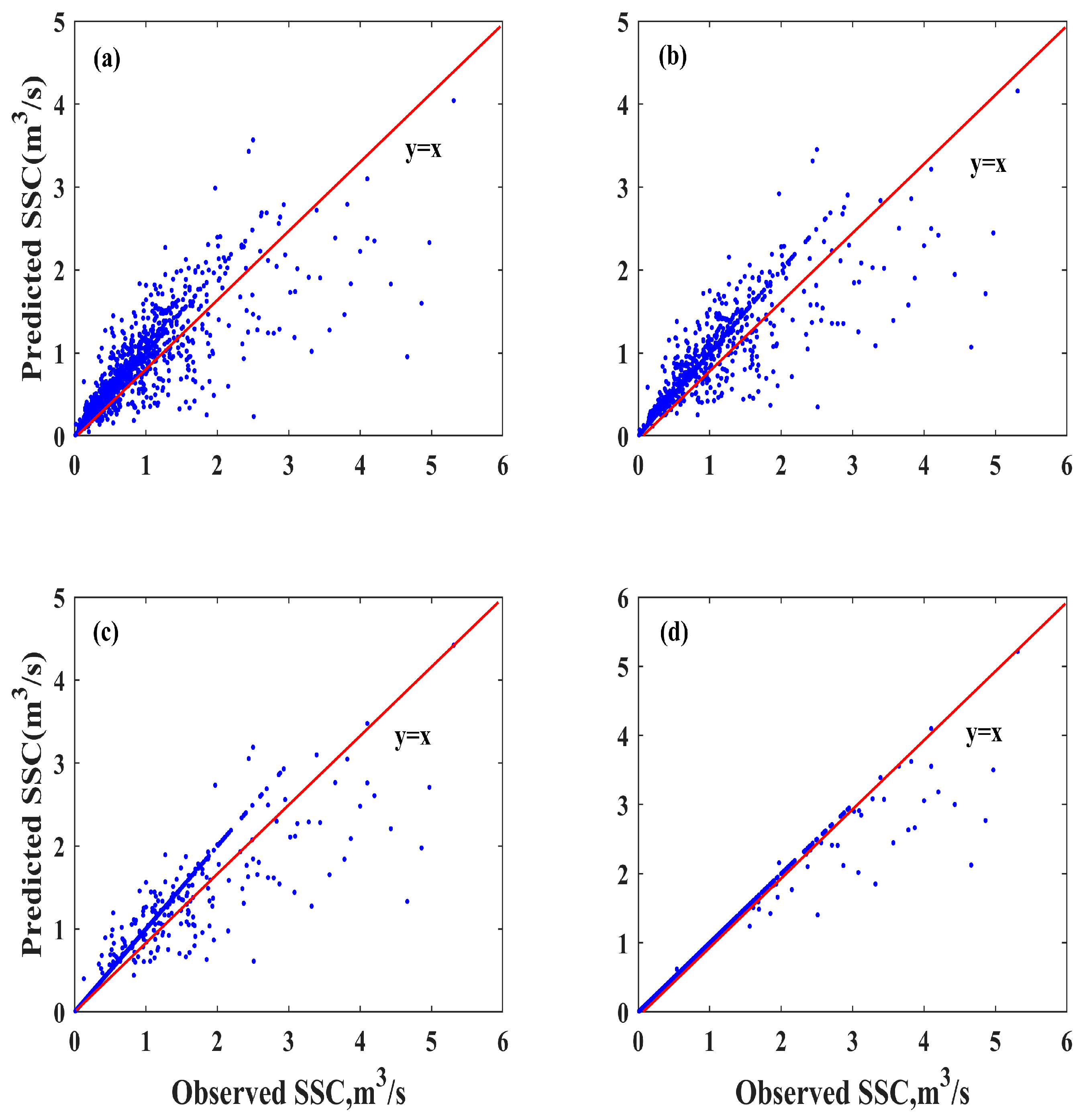
4.3.2. Performance Comparison and Ensemble Weighting Strategy
4.4. Comparative Evaluation of Model Variants and Optimization Strategies
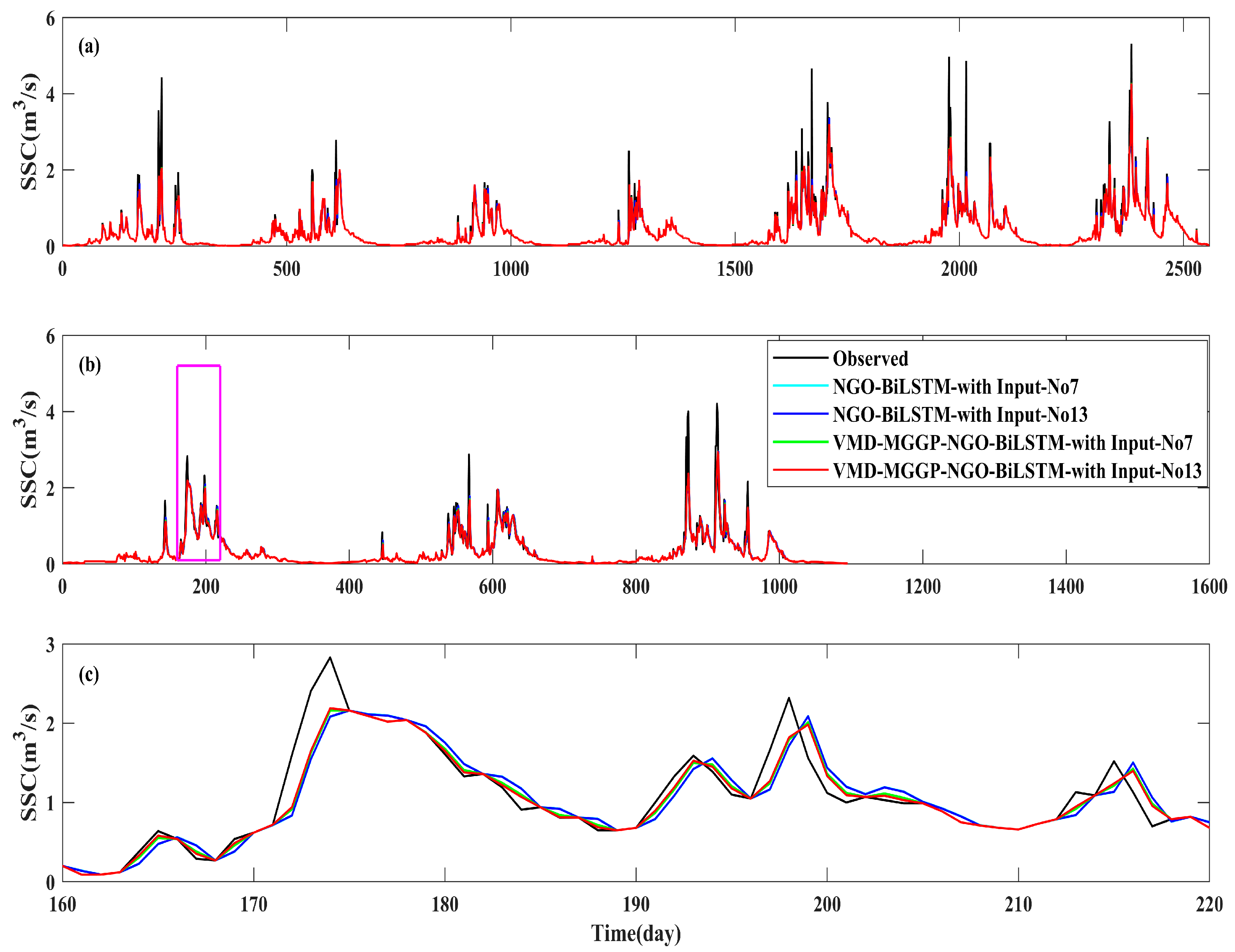
4.4.1. Impact of VMD-MGGP Integration on SSC Prediction Performance
4.4.2. The Influence of Adding NGO-ELM to SSC Prediction
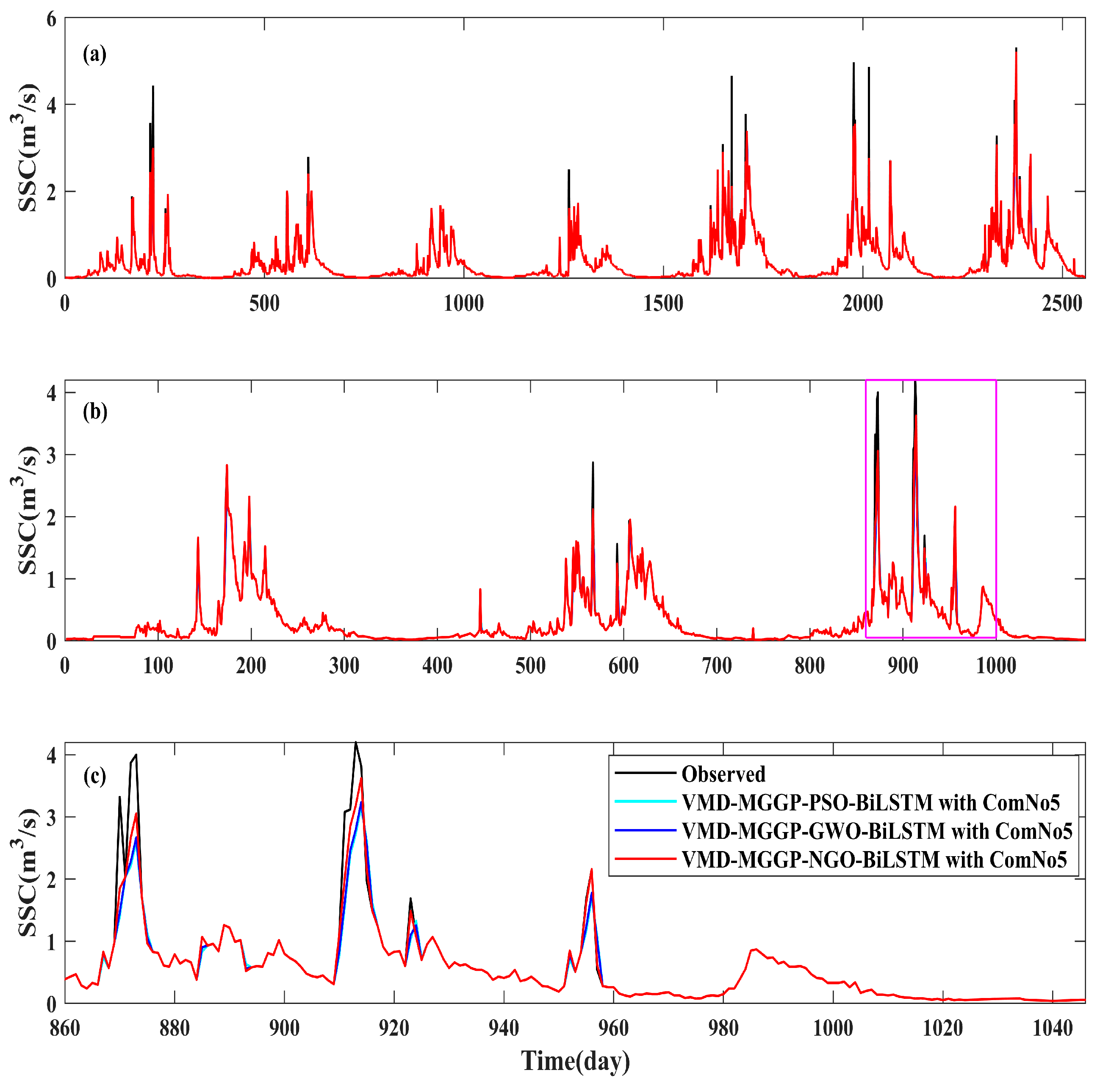
4.4.3. Evaluation of Different Optimization Algorithms: NGO vs. PSO and GWO
5. Discussion
6. Conclusions
- (1)
- The proposed model significantly outperformed classical machine learning baselines, achieving a 19.93% improvement in NSC over XGBoost and 15.26% over CNN-LSTM during the testing phase.
- (2)
- Compared to the averaging-based ensemble (VMD-MGGP-NGO- BiLSTM-AVE), the proposed NGO-optimized model achieved further performance gains—for instance, NSC increased by 7.91% for ComNo1 and 7.92% for ComNo2.
- (3)
- When replacing NGO with GWO and PSO in the ensemble optimization phase, the proposed model still maintained superior generalization, achieving an average NSC of 0.964, compared to 0.927 (GWO) and 0.909 (PSO), highlighting its robustness and adaptability in complex prediction tasks.
Author Contributions
Funding
Data Availability Statement
Acknowledgments
Conflicts of Interest
References
- Abramson, J.; Adler, J.; Dunger, J.; Evans, R.; Green, T.; Pritzel, A.; Ronneberger, O.; Willmore, L.; Ballard, A.J.; Bambrick, J.; et al. Accurate structure prediction of biomolecular interactions with AlphaFold 3. Nature 2024, 630, 493–500. [Google Scholar] [CrossRef] [PubMed]
- Agarwal, V.; Singh, B.V.R.; Marsh, S.; Qin, Z.; Sen, A.; Kulhari, K. Integrated remote sensing for enhanced drought assessment: A multi-index approach in Rajasthan, India. Earth Space Sci. 2025, 12, e2024EA003639. [Google Scholar] [CrossRef]
- Song, H.; Chen, Q.; Jiang, T.; Li, Y.; Li, X.; Xi, W.; Huang, S. Applying ensemble models based on graph neural network and reinforcement learning for wind power forecasting. arXiv 2025, arXiv:2501.16591. [Google Scholar]
- Haq, M.A. CDLSTM: A novel model for climate change forecasting. Comput. Mater. Contin. 2022, 71, 2363–2381. [Google Scholar]
- Alhuqayl, S.O.; Alenazi, A.T.; Alabduljabbar, H.A.; Haq, M.A. Improving Predictive Maintenance in Industrial Environments via IIoT and Machine Learning. Int. J. Adv. Comput. Sci. Appl. 2024, 15, 627–636. [Google Scholar] [CrossRef]
- Alabdulwahab, A.; Haq, M.A.; Alshehri, M. Cyberbullying detection using machine learning and deep learning. Int. J. Adv. Comput. Sci. Appl. 2023, 14, 424–432. [Google Scholar] [CrossRef]
- Haq, M.A.; Khan, M.Y.A. Crop water requirements with changing climate in an arid region of Saudi Arabia. Sustainability 2022, 14, 13554. [Google Scholar] [CrossRef]
- Haq, M.A. SMOTEDNN: A novel model for air pollution forecasting and AQI classification. Comput. Mater. Contin. 2022, 71, 1404–1425. [Google Scholar]
- Nguyen, B.Q.; Van Binh, D.; Tran, T.N.D.; Kantoush, S.A.; Sumi, T. Response of streamflow and sediment variability to cascade dam development and climate change in the Sai Gon Dong Nai River basin. Clim. Dyn. 2004, 62, 7997–8017. [Google Scholar] [CrossRef]
- Khosravi, K.; Golkarian, A.; Melesse, A.M.; Deo, R.C. Suspended sediment load modeling using advanced hybrid rotation forest based elastic network approach. J. Hydrol. 2022, 610, 127963. [Google Scholar] [CrossRef]
- Harrington, S.T.; Harrington, J.R. An assessment of the suspended sediment rating curve approach for load estimation on the Rivers Bandon and Owenabue, Ireland. Geomorphology 2013, 185, 27–38. [Google Scholar] [CrossRef]
- Zhang, W.; Wei, X.; Jinhai, Z.; Yuliang, Z.; Zhang, Y. Estimating suspended sediment loads in the Pearl River Delta region using sediment rating curves. Cont. Shelf Res. 2012, 38, 35–46. [Google Scholar] [CrossRef]
- Guillén, J.; Jiménez, J.A.; Palanques, A.; Gràcia, V.; Puig, P.; Sánchez-Arcilla, A. Sediment resuspension across a microtidal, low-energy inner shelf. Cont. Shelf Res. 2002, 22, 305–325. [Google Scholar] [CrossRef]
- Tseng, C.Y.; Tinoco, R.O. A two-layer turbulence-based model to predict suspended sediment concentration in flows with aquatic vegetation. Geophys. Res. Lett. 2021, 48, e2020GL091255. [Google Scholar] [CrossRef]
- Adnan, R.M.; Liang, Z.; Heddam, S.; Zounemat-Kermani, M.; Kisi, O.; Li, B. Least square support vector machine and multivariate adaptive regression splines for streamflow prediction in mountainous basin using hydro-meteorological data as inputs. J. Hydrol. 2020, 586, 124371. [Google Scholar] [CrossRef]
- Liu, G.; Guo, J.B. Bidirectional LSTM with attention mechanism and convolutional layer for text classification. Neurocomputing 2019, 337, 325–338. [Google Scholar] [CrossRef]
- Wu, B.; van Maren, D.S.; Li, L. Predictability of sediment transport in the Yellow River using selected transport formulas. Int. J. Sediment Res. 2008, 23, 283–298. [Google Scholar] [CrossRef]
- Kisi, O.; Zounemat-Kermani, M. Suspended Sediment Modeling Using Neuro-Fuzzy Embedded Fuzzy c-Means Clustering Technique. Water Resour. Manag. 2016, 30, 3979–3994. [Google Scholar] [CrossRef]
- Kaveh, K.; Kaveh, H.; Bui, M.D.; Rutschmann, P. Long short-term memory for predicting daily suspended sediment concentration. Eng. Comput. 2021, 37, 2013–2027. [Google Scholar] [CrossRef]
- Liu, Z.; Zhou, P.; Chen, X.; Guan, Y. A multivariate conditional model for streamflow prediction and spatial precipitation refinement. J. Geophys. Res. Atmos. 2015, 120, 10,116–10,129. [Google Scholar] [CrossRef]
- Marshall, S.R.; Tran, T.N.D.; Tapas, M.R.; Nguyen, B.Q. Integrating artificial intelligence and machine learning in hydrological modeling for sustainable resource management. Int. J. River Basin Manag. 2025, 1–17. [Google Scholar] [CrossRef]
- Gao, S.; Huang, Y.; Zhang, S.; Han, J.; Wang, G.; Zhang, M.; Lin, Q. Short-term runoff prediction with GRU and LSTM networks without requiring time step optimization during sample generation. J. Hydrol. 2020, 589, 125188. [Google Scholar] [CrossRef]
- Fang, L.Z.; Shao, D.G. Application of Long Short-Term Memory (LSTM) on the Prediction of Rainfall-Runoff in Karst Area. Front. Phys. 2022, 9, 790687. [Google Scholar] [CrossRef]
- Nourani, V.; Behfar, N. Multi-station runoff-sediment modeling using seasonal LSTM models. J. Hydrol. 2021, 601, 126672. [Google Scholar] [CrossRef]
- Li, S.C.; Xie, Q.C.; Yang, J. Daily suspended sediment forecast by an integrated dynamic neural network. J. Hydrol. 2022, 604, 127258. [Google Scholar] [CrossRef]
- Siami-Namini, S.; Tavakoli, N.; Namin, A.S. The Performance of LSTM and BiLSTM in Forecasting Time Series. In Proceedings of the 2019 IEEE International Conference on Big Data (Big Data), Los Angeles, CA, USA, 9–12 December 2019; pp. 3285–3292. [Google Scholar]
- Wang, J.; Wang, X.; Thiam Khu, S. A Decomposition-based Multi-model and Multiparameter Ensemble Forecast Framework for Monthly Streamflow Forecasting. J. Hydrol. 2023, 618, 129083. [Google Scholar] [CrossRef]
- Dhaka, P.; Nagpal, B. WoM-based deep BiLSTM: Smart disease prediction model using WoM-based deep BiLSTM classifier. Multimed. Tools Appl. 2023, 82, 25061–25082. [Google Scholar] [CrossRef]
- Xia, D.W.; Yang, N.; Jian, S.Y.; Hu, Y.; Li, H.Q. SW-BiLSTM: A Spark-based weighted BiLSTM model for traffic flow forecasting. Multimed. Tools Appl. 2022, 81, 23589–23614. [Google Scholar] [CrossRef]
- Ni, L.; Wang, D.; Wu, J.; Wang, Y.; Tao, Y.; Zhang, J.; Liu, J. Streamflow forecasting using extreme gradient boosting model coupled with Gaussian mixture model. J. Hydrol. 2020, 586, 124901. [Google Scholar] [CrossRef]
- Sun, N.; Zhou, J.; Chen, L.; Jia, B.; Tayyab, M.; Peng, T. An adaptive dynamic short-term wind speed forecasting model using secondary decomposition and an improved regularized extreme learning machine. Energy 2018, 165, 939–957. [Google Scholar] [CrossRef]
- Banaie-Dezfouli, M.; Nadimi-Shahraki, M.H.; Beheshti, Z. R-GWO: Representative-based grey wolf optimizer for solving engineering problems. Appl. Soft. Comput. 2021, 106, 107328. [Google Scholar] [CrossRef]
- Ch, S.; Anand, N.; Panigrahi, B.K.; Mathur, S. Streamflow forecasting by SVM with quantum behaved particle swarm optimization. Neurocomputing 2013, 101, 18–23. [Google Scholar] [CrossRef]
- Cui, J.K.; Liu, T.Y.; Zhu, M.C.; Xu, Z.B. Improved team learning-based grey wolf optimizer for optimization tasks and engineering problems. J. Supercomput. 2023, 79, 10864–10914. [Google Scholar] [CrossRef]
- Faris, H.; Aljarah, I.; Al-Betar, M.A.; Mirjalili, S. Grey wolf optimizer: A review of recent variants and applications. Neural Comput. Appl. 2018, 30, 413–435. [Google Scholar] [CrossRef]
- Hong, M.; Wang, D.; Wang, Y.; Zeng, X.; Ge, S.; Yan, H.; Singh, V.P. Mid- and long- term runoff predictions by an improved phase-space reconstruction model. Environ. Res. 2016, 148, 560–573. [Google Scholar] [CrossRef]
- Lalbakhsh, A.; Afzal, M.U.; Esselle, K.P. Multiobjective Particle Swarm Optimization to Design a Time-Delay Equalizer Metasurface for an Electromagnetic Band-Gap Resonator Antenna. IEEE Antennas Wirel. Propag. Lett. 2017, 16, 912–915. [Google Scholar] [CrossRef]
- Nadimi-Shahraki, M.H.; Taghian, S.; Mirjalili, S. An improved grey wolf optimizer for solving engineering problems. Expert Syst. Appl. 2021, 166, 113917. [Google Scholar] [CrossRef]
- Sedki, A.; Ouazar, D.; El Mazoudi, E. Evolving neural network using real coded genetic algorithm for daily rainfall–runoff forecasting. Expert Syst. Appl. 2009, 36, 4523–4527. [Google Scholar] [CrossRef]
- Tikhamarine, Y.; Souag-Gamane, D.; Najah Ahmed, A.; Kisi, O.; El-Shafie, A. Improving artificial intelligence models accuracy for monthly streamflow forecasting using grey Wolf optimization (GWO) algorithm. J. Hydrol. 2020, 582, 124435. [Google Scholar] [CrossRef]
- Dehghani, M.; Hubalovsky, S.; Trojovsky, P. Northern Goshawk Optimization: A New Swarm-Based Algorithm for Solving Optimization Problems. IEEE Access 2021, 9, 162059–162080. [Google Scholar] [CrossRef]
- El-Dabah, M.A.; El-Sehiemy, R.A.; Hasanien, H.M.; Saad, B. Photovoltaic model parameters identification using Northern Goshawk Optimization algorithm. Energy 2023, 262, 125522. [Google Scholar] [CrossRef]
- Jasim, M.J.M.; Hussan, B.K.; Zeebaree, S.R.M.; Ageed, Z.S. Automated Colonic Polyp Detection and Classification Enabled Northern Goshawk Optimization with Deep Learning. CMC-Comput. Mater. Contin. 2023, 75, 3677–3693. [Google Scholar] [CrossRef]
- Wen, X.; Feng, Q.; Deo, R.C.; Wu, M.; Yin, Z.; Yang, L.; Singh, V.P. Two-phase extreme learning machines integrated with the complete ensemble empirical mode decomposition with adaptive noise algorithm for multi-scale runoff prediction problems. J. Hydrol. 2019, 570, 167–184. [Google Scholar] [CrossRef]
- Mi, X.; Zhao, S. Wind speed prediction based on singular spectrum analysis and neural network structural learning. Energ. Convers. Manag. 2020, 216, 112956. [Google Scholar] [CrossRef]
- Zhao, X.; Chen, X.; Huang, Q. Trend and long-range correlation characteristics analysis of runoff in upper Fenhe River basin. Water Resour. 2017, 44, 31–42. [Google Scholar] [CrossRef]
- Ali, M.; Prasad, R. Significant wave height forecasting via an extreme learningmachine model integrated with improved complete ensemble empirical mode decomposition. Renew. Sustain. Energy Rev. 2019, 104, 281–295. [Google Scholar] [CrossRef]
- Dragomiretskiy, K.; Zosso, D. Variational Mode Decomposition. IEEE Trans. Signal Process. 2014, 62, 531–544. [Google Scholar] [CrossRef]
- Karaaslan, O.F.; Bilgin, G. Comparison of Variational Mode Decomposition and Empirical Mode Decomposition Features for Cell Segmentation in Histopathological Images. In Proceedings of the 2020 Medical Technologies Congress (TIPTEKNO), Online, 19–20 November 2020. [Google Scholar]
- Lian, J.J.; Liu, Z.; Wang, H.J.; Dong, X.F. Adaptive variational mode decomposition method for signal processing based on mode characteristic. Mech. Syst. Signal Process. 2018, 107, 53–77. [Google Scholar] [CrossRef]
- Malhotra, V.; Sandhu, M.K. Electrocardiogram signals denoising using improved variational mode decomposition. J. Med. Signals Sens. 2021, 11, 100–107. [Google Scholar] [CrossRef]
- Palanisamy, T. Smoothing the difference-based estimates of variance using variational mode decomposition. Commun. Stat.-Simul. Comput. 2017, 46, 4991–5001. [Google Scholar] [CrossRef]
- Rahul, S.; Sunitha, R. Dominant Electromechanical Oscillation Mode Identification using Modified Variational Mode Decomposition. Arab. J. Sci. Eng. 2021, 46, 10007–10021. [Google Scholar] [CrossRef]
- Wang, J.Y.; Li, J.G.; Wang, H.T.; Guo, L.X. Composite fault diagnosis of gearbox based on empirical mode decomposition and improved variational mode decomposition. J. Low Freq. Noise Vib. Act. Control. 2021, 40, 332–346. [Google Scholar] [CrossRef]
- Yue, Y.; Sun, G.; Cai, Y.; Chen, R.; Wang, X.; Zhang, S. Comparison of performances of variational mode decomposition and empirical mode decomposition. In Proceedings of the 3rd International Conference on Energy Science and Applied Technology (ESAT 2016), Wuhan, China, 25–26 June 2016; pp. 469–476. [Google Scholar]
- Fan, J.; Liu, X.; Li, W. Daily suspended sediment concentration forecast in the upper reach of Yellow River using a comprehensive integrated deep learning model. J. Hydrol. 2023, 623, 129732. [Google Scholar] [CrossRef]
- Wang, H.S.; Zhang, Y.P.; Liang, J.; Liu, L.L. DAFA-BiLSTM: Deep Autoregression Feature Augmented Bidirectional LSTM network for time series prediction. Neural Netw. 2023, 157, 240–256. [Google Scholar] [CrossRef]
- Liu, X.; Li, W. MGC-LSTM: A deep learning model based on graph convolution of multiple graphs for PM2.5 prediction. Int. J. Environ. Sci. Technol. 2023, 20, 10297–10312. [Google Scholar] [CrossRef]
- Zhang, X.Q.; Wang, X.; Li, H.Y.; Sun, S.F.; Liu, F. Monthly runoff prediction based on a coupled VMD-SSA-BiLSTM model. Sci. Rep. 2023, 13, 13149. [Google Scholar] [CrossRef]
- Huang, C.C.; Chang, M.J.; Lin, G.F.; Wu, M.C.; Wang, P.H. Real-time forecasting of suspended sediment concentrations reservoirs by the optimal integration of multiple machine learning techniques. J. Hydrol.-Reg. Stud. 2021, 34, 100804. [Google Scholar] [CrossRef]
- Searson, D.P.; Willis, M.J.; Montague, G.A. GPTIPS: An open-source genetic programming toolbox for multigene symbolic regression. Proc. Int. Multi-Conf. Eng. Comput. Sci. 2010, 1, 77–80. [Google Scholar]
- Bengio, Y.; Simard, P.; Frasconi, P. Learning long-term dependencies with gradient descent is difficult. IEEE Trans. Neural Netw. 1994, 5, 157–166. [Google Scholar] [CrossRef]
- Gers, F.A.; Schmidhuber, J.; Cummins, F. Learning to forget: Continual prediction with LSTM. In Proceedings of the 1999 Ninth International Conference on Artificial Neural Networks ICANN 99. (Conf. Publ. No. 470), Edinburgh, UK, 7–10 September 1999; Volume 2, pp. 850–855. [Google Scholar] [CrossRef]
- Dehghani, M. Northern Goshawk Optimization: A New Swarm-Based Algorithm MATLAB Central File Exchang. 2023. Available online: https://www.mathworks.com/matlabcentral/fileexchange/106665-northern-goshawk-optimization-a-new-swarm-based-algorithm (accessed on 12 February 2022).
- Moriasi, D.N.; Arnold, J.G.; van Liew, M.W.; Bingner, R.L.; Harmel, R.D.; Veith, T.L. Model Evaluation Guidelines for Systematic Quantification of Accuracy in Watershed Simulations. Trans. ASABE 2007, 50, 885–900. [Google Scholar] [CrossRef]
- Khan, M.M.H.; Muhammad, N.S.; El-Shafie, A. Wavelet based hybrid ANN-ARIMA models for meteorological drought forecasting. J. Hydrol. 2020, 590, 125380. [Google Scholar] [CrossRef]
- Adaryani, F.R.; Mousavi, S.J.; Jafari, F. Short-term rainfall forecasting using machine learning-based approaches of PSO-SVR, LSTM and CNN. J. Hydrol. 2022, 614, 128463. [Google Scholar] [CrossRef]
- Xu, J.; Anctil, F.; Boucher, M.A. Exploring hydrologic post-processing of ensemble stream flow forecasts based on Affine kernel dressing and Nondominated sorting genetic algorithm II. Hydrol. Earth Syst. Sci. Discuss. 2020, 2020, 1–34. [Google Scholar] [CrossRef]
- Troin, M.; Arsenault, R.; Wood, A.W.; Brissette, F.; Martel, J.L. Generating Ensemble Streamflow Forecasts: A Review of Methods and Approaches Over the Past 40 Years. Water Resour. Res. 2021, 57, e2020WR028392. [Google Scholar] [CrossRef]
- Zhang, S.; Wu, J.; Wang, Y.G.; Jeng, D.S.; Li, G. A physics-informed statistical learning framework for forecasting local suspended sediment concentrations in marine environment. Water Res. 2022, 218, 118518. [Google Scholar] [CrossRef]
- Zuo, G.; Luo, J.; Wang, N.; Lian, Y.; He, X. Decomposition ensemble model based on variational mode decomposition and long short-term memory for streamflow forecasting. J. Hydrol. 2020, 585, 124776. [Google Scholar] [CrossRef]
- Tian, Z.D. Modes decomposition forecasting approach for ultra-short-term wind speed. Appl. Soft. Comput. 2021, 105, 107303. [Google Scholar] [CrossRef]
- Sun, Z.X.; Zhao, M.Y.; Zhao, G.H. Hybrid model based on VMD decomposition, clustering analysis, long short memory network, ensemble learning and error complementation for short-term wind speed forecasting assisted by Flink platform. Energy 2022, 261, 125248. [Google Scholar] [CrossRef]
- Samantaray, S.; Sahoo, A.; Ghose, D.K. Assessment of Sediment Load Concentration Using SVM, SVM-FFA and PSR-SVM-FFA in Arid Watershed, India: A Case Study. KSCE J. Civ. Eng. 2020, 24, 1944–1957. [Google Scholar] [CrossRef]
- Serra, T.; Soler, M.; Barcelona, A.; Colomer, J. Suspended sediment transport and deposition in sediment-replenished artificial floods in Mediterranean rivers. J. Hydrol. 2022, 609, 127756. [Google Scholar] [CrossRef]
- Sudheer, K.P.; Gosain, A.K.; Ramasastri, K.S. A data-driven algorithm for constructing artificial neural network rainfall-runoff models. Hydrol. Process. 2002, 16, 1325–1330. [Google Scholar] [CrossRef]
- Yu, M.; Niu, D.; Gao, T.; Wang, K.; Sun, L.; Li, M.; Xu, X. A novel framework for ultra-short-term interval wind power prediction based on RF-WOA-VMD and BiGRU optimized by the attention mechanism. Energy 2023, 269, 126738. [Google Scholar] [CrossRef]
- Zang, H.; Liu, L.; Sun, L.; Cheng, L.; Wei, Z.; Sun, G. Short-term global horizontal irradiance forecasting based on a hybrid CNN-LSTM model with spatiotemporal correlations. Renew. Energy 2020, 160, 26–41. [Google Scholar] [CrossRef]


| Period | Variables | Mean | Standard Deviation | Coefficient of Variation | Skewness | Maximum | Minimum |
|---|---|---|---|---|---|---|---|
| Training | Flow (m3s−1) | 741.56 | 682 | 0.93 | 1.993 | 5390 | 108 |
| SSC (kgl−1) | 0.3723 | 0.5193 | 1.44 | 2.222 | 5.31 | 0.011 | |
| Testing | Flow (m3s−1) | 630.4 | 507.02 | 0.82 | 1.354 | 2620 | 147 |
| SSC (kgl−1) | 0.3462 | 0.5939 | 1.71 | 2.942 | 4.20 | 0.013 |
| No. | Vector | No. | Vector |
|---|---|---|---|
| Input-No1 | Q(t) | Input-No14 | SSC(t−1), SSC(t−2), SSC(t−3), Q(t−1), Q(t−2), Q(t−3) |
| Input-No2 | SSC(t−1) | Input-No15 | SSC(t−1), SSC(t−2), SSC(t−4), Q(t−1), Q(t−2), Q(t−4) |
| Input-No3 | SSC(t−1), Q(t) | Input-No16 | SSC(t−1), SSC(t−3), SSC(t−4), Q(t−1), Q(t−3), Q(t−4) |
| Input-No4 | SSC(t−1), Q(t−1) | Input-No17 | SSC(t−2), SSC(t−3), SSC(t−4), Q(t−2), Q(t−3), Q(t−4) |
| Input-No5 | SSC(t−2), Q(t−2) | Input-No18 | SSC(t−1), SSC(t−2), SSC(t−3), SSC(t−4), Q(t−1), Q(t−2), Q(t−3), Q(t−4) |
| Input-No6 | SSC(t−3), Q(t−3) | Input-No19 | SSC(t−1), Q(t), Q(t−1) |
| Input-No7 | SSC(t−4), Q(t−4) | Input-No20 | SSC(t−1), SSC(t−2), Q(t), Q(t−1), Q(t−2) |
| Input-No8 | SSC(t−1), SSC(t−2), Q(t−1), Q(t-2 | Input-No21 | SSC(t−1), SSC(t−3), Q(t), Q(t−1), Q(t−3) |
| Input-No9 | SSC(t−1), SSC(t−3), Q(t−1), Q(t−3) | Input-No22 | SSC(t−1), SSC(t−4), Q(t), Q(t−1), Q(t−4) |
| Input-No10 | SSC(t−1), SSC(t−4), Q(t−1), Q(t−4) | Input-No23 | SSC(t−1), SSC(t−2), SSC(t−3), Q(t), Q(t−1), Q(t−2), Q(t−3) |
| Input-No11 | SSC(t−2), SSC(t−3), Q(t−2), Q(t−3) | Input-No24 | SSC(t−1), SSC(t−2), SSC(t−4), Q(t), Q(t−1), Q(t−2), Q(t−4) |
| Input-No12 | SSC(t−2), SSC(t−4), Q(t−4), Q(t−2) | Input-No25 | SSC(t−1), SSC(t−3), SSC(t−4), Q(t), Q(t−1), Q(t−3), Q(t−4) |
| Input-No13 | SSC(t−3), SSC(t−4), Q(t−3), Q(t−4) | Input-No26 | SSC(t−1), SSC(t−2), SSC(t−3), SSC(t−4), Q(t), Q(t−1), Q(t−2), Q(t−3), Q(t−4) |
| Parameter | Value | Parameter | Value |
|---|---|---|---|
| MaxEpochs | 300 | Epsilon | 1.0 × 10⁻⁸ |
| InterationsPerEpoch | 1 | GradientThresholdMethod | l2norm |
| MaxInterations | 300 | GradientThreshold | 1 |
| Optimizer | adam | LearnRateSchedule | piecewise |
| InitialLearnRate | * | LearnRateDropFactor | 0.8 |
| DropoutLayerProbability | * | Number of hidden_units | * |
| Model Inputs | Training | Testing | ||||||
|---|---|---|---|---|---|---|---|---|
| MAE | RMSE | NSC | R2 | MAE | RMSE | NSC | R2 | |
| Input-No1 | 0.0351 | 0.1943 | 0.8712 | 0.8712 | 0.0396 | 0.1806 | 0.8619 | 0.8619 |
| Input-No2 | 0.0296 | 0.1824 | 0.8865 | 0.8865 | 0.0314 | 0.1655 | 0.8841 | 0.8841 |
| Input-No3 | 0.0284 | 0.1795 | 0.8901 | 0.8901 | 0.0306 | 0.1636 | 0.8867 | 0.8867 |
| Input-No4 | 0.0333 | 0.1905 | 0.8762 | 0.8762 | 0.0394 | 0.1803 | 0.8624 | 0.8624 |
| Input-No5 | 0.0331 | 0.1900 | 0.8768 | 0.8768 | 0.0370 | 0.1761 | 0.8687 | 0.8687 |
| Input-No6 | 0.0311 | 0.1859 | 0.8821 | 0.8821 | 0.0342 | 0.1710 | 0.8762 | 0.8762 |
| Input-No7 | 0.0311 | 0.1859 | 0.8821 | 0.8821 | 0.0403 | 0.1818 | 0.8601 | 0.8601 |
| Input-No8 | 0.0277 | 0.1778 | 0.8921 | 0.8921 | 0.0356 | 0.1737 | 0.8723 | 0.8723 |
| Input-No9 | 0.0277 | 0.1778 | 0.8921 | 0.8921 | 0.0317 | 0.1661 | 0.8832 | 0.8832 |
| Input-No10 | 0.0307 | 0.1850 | 0.8832 | 0.8832 | 0.0340 | 0.1707 | 0.8767 | 0.8767 |
| Input-No11 | 0.0229 | 0.1649 | 0.9072 | 0.9072 | 0.0270 | 0.1547 | 0.8987 | 0.8987 |
| Input-No12 | 0.0348 | 0.1936 | 0.8721 | 0.8721 | 0.0360 | 0.1745 | 0.8711 | 0.8711 |
| Input-No13 | 0.0320 | 0.1877 | 0.8798 | 0.8798 | 0.0366 | 0.1755 | 0.8697 | 0.8697 |
| Input-No14 | 0.0307 | 0.1849 | 0.8834 | 0.8834 | 0.0361 | 0.1746 | 0.8710 | 0.8710 |
| Input-No15 | 0.0341 | 0.1922 | 0.8740 | 0.8740 | 0.0400 | 0.1812 | 0.8610 | 0.8610 |
| Input-No16 | 0.0264 | 0.1744 | 0.8962 | 0.8962 | 0.0343 | 0.1712 | 0.8759 | 0.8759 |
| Input-No17 | 0.0342 | 0.1925 | 0.8736 | 0.8736 | 0.0441 | 0.1874 | 0.8513 | 0.8513 |
| Input-No18 | 0.0374 | 0.1986 | 0.8654 | 0.8654 | 0.0425 | 0.1850 | 0.8551 | 0.8551 |
| Input-No19 | 0.0306 | 0.1846 | 0.8837 | 0.8837 | 0.0336 | 0.1700 | 0.8776 | 0.8776 |
| Input-No20 | 0.0319 | 0.1875 | 0.8801 | 0.8801 | 0.0343 | 0.1713 | 0.8758 | 0.8758 |
| Input-No21 | 0.0333 | 0.1906 | 0.8761 | 0.8761 | 0.0407 | 0.1824 | 0.8592 | 0.8592 |
| Input-No22 | 0.0347 | 0.1935 | 0.8723 | 0.8723 | 0.0355 | 0.1735 | 0.8726 | 0.8726 |
| Input-No23 | 0.0294 | 0.1819 | 0.8871 | 0.8871 | 0.0334 | 0.1696 | 0.8782 | 0.8782 |
| Input-No24 | 0.0267 | 0.1753 | 0.8952 | 0.8952 | 0.0360 | 0.1745 | 0.8711 | 0.8711 |
| Input-No25 | 0.0309 | 0.1853 | 0.8829 | 0.8829 | 0.0350 | 0.1727 | 0.8738 | 0.8738 |
| Input-No26 | 0.0332 | 0.1903 | 0.8764 | 0.8764 | 0.0391 | 0.1798 | 0.8632 | 0.8632 |
| Model Inputs | Weight of Input Vectors by NGO | |||||||||||
|---|---|---|---|---|---|---|---|---|---|---|---|---|
| 1 | 2 | 3 | 4 | 5 | 6 | 7 | 8 | 9 | 10 | 11 | 12 | |
| ComNo1 | 0.301 | 0.376 | 0.331 | |||||||||
| ComNo2 | 0.258 | 0.104 | 0.321 | 0.123 | ||||||||
| ComNo3 | 0.210 | 0.233 | 0.156 | 0.178 | 0.156 | |||||||
| ComNo4 | 0.139 | 0.128 | 0.161 | 0.141 | 0.108 | 0.128 | ||||||
| ComNo5 | 0.137 | 0.121 | 0.143 | 0.101 | 0.123 | 0.138 | 0.134 | |||||
| ComNo6 | 0.152 | 0.109 | 0.192 | 0.132 | 0.146 | 0.128 | 0.145 | 0.099 | ||||
| ComNo7 | 0.142 | 0.123 | 0.101 | 0.105 | 0.135 | 0.123 | 0.108 | 0.132 | 0.107 | |||
| ComNo8 | 0.123 | 0.125 | 0.135 | 0.141 | 0.126 | 0.101 | 0.099 | 0.128 | 0.092 | 0.093 | ||
| ComNo9 | 0.114 | 0.135 | 0.102 | 0.103 | 0.084 | 0.091 | 0.106 | 0.102 | 0.115 | 0.118 | 0.101 | |
| ComNo10 | 0.121 | 0.104 | 0.143 | 0.112 | 0.123 | 0.111 | 0.115 | 0.127 | 0.107 | 0.132 | 0.120 | 0.098 |
| Model Inputs | Training | Testing | ||||||
|---|---|---|---|---|---|---|---|---|
| MAE | RMSE | NSC | R2 | MAE | RMSE | NSC | R2 | |
| ComNo1 | 0.0067 | 0.0935 | 0.9702 | 0.9702 | 0.0090 | 0.0918 | 0.9643 | 0.9643 |
| ComNo2 | 0.0068 | 0.0941 | 0.9698 | 0.9698 | 0.0094 | 0.0939 | 0.9627 | 0.9627 |
| ComNo3 | 0.0078 | 0.1004 | 0.9656 | 0.9656 | 0.0092 | 0.0929 | 0.9635 | 0.9635 |
| ComNo4 | 0.0075 | 0.0986 | 0.9668 | 0.9668 | 0.0095 | 0.0944 | 0.9623 | 0.9623 |
| ComNo5 | 0.0059 | 0.0886 | 0.9732 | 0.9732 | 0.0073 | 0.0831 | 0.9708 | 0.9708 |
| ComNo6 | 0.0069 | 0.0947 | 0.9694 | 0.9694 | 0.0099 | 0.0962 | 0.9608 | 0.9608 |
| ComNo7 | 0.0071 | 0.0962 | 0.9684 | 0.9684 | 0.0087 | 0.0904 | 0.9654 | 0.9654 |
| ComNo8 | 0.0071 | 0.0959 | 0.9686 | 0.9686 | 0.0089 | 0.0916 | 0.9645 | 0.9645 |
| ComNo9 | 0.0080 | 0.1017 | 0.9647 | 0.9647 | 0.0092 | 0.0930 | 0.9634 | 0.9634 |
| ComNo10 | 0.0079 | 0.1011 | 0.9651 | 0.9651 | 0.0095 | 0.0944 | 0.9623 | 0.9623 |
| Prediction Model | Training | Testing | ||||||
|---|---|---|---|---|---|---|---|---|
| MAE | RMSE | NSC | R2 | MAE | RMSE | NSC | R2 | |
| XGBoost | 0.0641 | 0.2359 | 0.8102 | 0.8102 | 0.0681 | 0.2121 | 0.8095 | 0.8095 |
| CNN-LSTM | 0.0431 | 0.2088 | 0.8513 | 0.8513 | 0.0484 | 0.1930 | 0.8423 | 0.8423 |
| VMD-MGGP-NGO-BiLSTM | 0.0229 | 0.1649 | 0.9072 | 0.9072 | 0.0270 | 0.1547 | 0.8987 | 0.8987 |
| VMD-MGGP-NGO-BiLSTM-NGO | 0.0059 | 0.0886 | 0.9732 | 0.9732 | 0.0073 | 0.0831 | 0.9708 | 0.9708 |
| Model Inputs | Training | Testing | ||||||
|---|---|---|---|---|---|---|---|---|
| MAE | RMSE | NSC | R2 | MAE | RMSE | NSC | R2 | |
| Input-No1 | 0.0568 | 0.2282 | 0.8223 | 0.8223 | 0.0607 | 0.2061 | 0.8201 | 0.8201 |
| Input-No2 | 0.0519 | 0.2222 | 0.8315 | 0.8315 | 0.0616 | 0.2069 | 0.8187 | 0.8187 |
| Input-No3 | 0.0551 | 0.2262 | 0.8254 | 0.8254 | 0.0601 | 0.2056 | 0.8211 | 0.8211 |
| Input-No4 | 0.0516 | 0.2218 | 0.8321 | 0.8321 | 0.0560 | 0.2016 | 0.8279 | 0.8279 |
| Input-No5 | 0.0527 | 0.2233 | 0.8299 | 0.8299 | 0.0608 | 0.2062 | 0.8200 | 0.8200 |
| Input-No6 | 0.0516 | 0.2218 | 0.8321 | 0.8321 | 0.0568 | 0.2024 | 0.8265 | 0.8265 |
| Input-No7 | 0.0496 | 0.2191 | 0.8362 | 0.8362 | 0.0556 | 0.2012 | 0.8286 | 0.8286 |
| Input-No8 | 0.0528 | 0.2234 | 0.8297 | 0.8297 | 0.0581 | 0.2037 | 0.8243 | 0.8243 |
| Input-No9 | 0.0557 | 0.2269 | 0.8243 | 0.8243 | 0.0606 | 0.2060 | 0.8203 | 0.8203 |
| Input-No10 | 0.0516 | 0.2218 | 0.8321 | 0.8321 | 0.0553 | 0.2009 | 0.8291 | 0.8291 |
| Input-No11 | 0.0192 | 0.1530 | 0.9201 | 0.9201 | 0.0611 | 0.2064 | 0.8195 | 0.8195 |
| Input-No12 | 0.0568 | 0.2282 | 0.8223 | 0.8223 | 0.0617 | 0.2070 | 0.8186 | 0.8186 |
| Input-No13 | 0.0502 | 0.2198 | 0.8351 | 0.8351 | 0.0548 | 0.2003 | 0.8301 | 0.8301 |
| Input-No14 | 0.0557 | 0.2269 | 0.8244 | 0.8244 | 0.0595 | 0.2050 | 0.8220 | 0.8220 |
| Input-No15 | 0.0516 | 0.2218 | 0.8322 | 0.8322 | 0.0545 | 0.2001 | 0.8305 | 0.8305 |
| Input-No16 | 0.0624 | 0.2342 | 0.8128 | 0.8128 | 0.0687 | 0.2126 | 0.8087 | 0.8087 |
| Input-No17 | 0.0628 | 0.2346 | 0.8123 | 0.8123 | 0.0695 | 0.2132 | 0.8075 | 0.8075 |
| Input-No18 | 0.0580 | 0.2296 | 0.8202 | 0.8202 | 0.0661 | 0.2106 | 0.8122 | 0.8122 |
| Input-No19 | 0.0555 | 0.2267 | 0.8246 | 0.8246 | 0.0606 | 0.2060 | 0.8203 | 0.8203 |
| Input-No20 | 0.0504 | 0.2202 | 0.8346 | 0.8346 | 0.0556 | 0.2012 | 0.8287 | 0.8287 |
| Input-No21 | 0.0505 | 0.2203 | 0.8345 | 0.8345 | 0.0543 | 0.1999 | 0.8309 | 0.8309 |
| Input-No22 | 0.0540 | 0.2249 | 0.8275 | 0.8275 | 0.0589 | 0.2044 | 0.8231 | 0.8231 |
| Input-No23 | 0.0497 | 0.2192 | 0.8361 | 0.8361 | 0.0544 | 0.2000 | 0.8307 | 0.8307 |
| Input-No24 | 0.0479 | 0.2165 | 0.8401 | 0.8401 | 0.0537 | 0.1991 | 0.8321 | 0.8321 |
| Input-No25 | 0.0524 | 0.2228 | 0.8306 | 0.8306 | 0.0569 | 0.2025 | 0.8263 | 0.8263 |
| Input-No26 | 0.0526 | 0.2232 | 0.8301 | 0.8301 | 0.0589 | 0.2044 | 0.8231 | 0.8231 |
| Model Inputs | Testing | |||
|---|---|---|---|---|
| MAE | RMSE | NSC | R2 | |
| Input-No1 | −34.76% | −12.37% | 5.10% | 5.10% |
| Input-No2 | −49.03% | −20.01% | 7.99% | 7.99% |
| Input-No3 | −49.08% | −20.43% | 7.99% | 7.99% |
| Input-No4 | −29.64% | −10.57% | 4.17% | 4.17% |
| Input-No5 | −39.14% | −14.60% | 5.94% | 5.94% |
| Input-No6 | −39.79% | −15.51% | 6.01% | 6.01% |
| Input-No7 | −27.52% | −9.64% | 3.80% | 3.80% |
| Input-No8 | −38.73% | −14.73% | 5.82% | 5.82% |
| Input-No9 | −47.69% | −19.37% | 7.67% | 7.67% |
| Input-No10 | −38.52% | −15.03% | 5.74% | 5.74% |
| Input-No11 | −55.81% | −25.05% | 9.66% | 9.66% |
| Input-No12 | −41.65% | −15.70% | 6.41% | 6.41% |
| Input-No13 | −33.21% | −12.38% | 4.77% | 4.77% |
| Input-No14 | −39.33% | −14.83% | 5.96% | 5.96% |
| Input-No15 | −26.61% | −9.45% | 3.67% | 3.67% |
| Input-No16 | −50.07% | −19.47% | 8.31% | 8.31% |
| Input-No17 | −36.55% | −12.10% | 5.42% | 5.42% |
| Input-No18 | −35.70% | −12.16% | 5.28% | 5.28% |
| Input-No19 | −44.55% | −17.48% | 6.99% | 6.99% |
| Input-No20 | −38.31% | −14.86% | 5.68% | 5.68% |
| Input-No21 | −25.05% | −8.75% | 3.41% | 3.41% |
| Input-No22 | −39.73% | −15.12% | 6.01% | 6.01% |
| Input-No23 | −38.60% | −15.20% | 5.72% | 5.72% |
| Input-No24 | −32.96% | −12.36% | 4.69% | 4.69% |
| Input-No25 | −38.49% | −14.72% | 5.75% | 5.75% |
| Input-No26 | −33.62% | −12.04% | 4.87% | 4.87% |
| Average | −38.62% | −14.77% | 5.88% | 5.88% |
| Model Inputs | Training | Testing | ||||||
|---|---|---|---|---|---|---|---|---|
| MAE | RMSE | NSC | R2 | MAE | RMSE | NSC | R2 | |
| ComNo1 | 0.0270 | 0.1760 | 0.8943 | 0.8943 | 0.0295 | 0.1610 | 0.8902 | 0.8902 |
| ComNo2 | 0.0261 | 0.1737 | 0.8971 | 0.8971 | 0.0289 | 0.1596 | 0.8921 | 0.8921 |
| ComNo3 | 0.0260 | 0.1735 | 0.8973 | 0.8973 | 0.0295 | 0.1610 | 0.8903 | 0.8903 |
| ComNo4 | 0.0282 | 0.1790 | 0.8907 | 0.8907 | 0.0292 | 0.1604 | 0.8911 | 0.8911 |
| ComNo5 | 0.0249 | 0.1704 | 0.9009 | 0.9009 | 0.0260 | 0.1519 | 0.9023 | 0.9023 |
| ComNo6 | 0.0274 | 0.1770 | 0.8931 | 0.8931 | 0.0295 | 0.1611 | 0.8901 | 0.8901 |
| ComNo7 | 0.0278 | 0.1780 | 0.8919 | 0.8919 | 0.0291 | 0.1601 | 0.8915 | 0.8915 |
| ComNo8 | 0.0272 | 0.1765 | 0.8937 | 0.8937 | 0.0348 | 0.1722 | 0.8745 | 0.8745 |
| ComNo9 | 0.0269 | 0.1758 | 0.8945 | 0.8945 | 0.0283 | 0.1582 | 0.8941 | 0.8941 |
| ComNo10 | 0.0265 | 0.1747 | 0.8959 | 0.8959 | 0.0289 | 0.1596 | 0.8921 | 0.8921 |
| Model Inputs | Training | Testing | ||||||
|---|---|---|---|---|---|---|---|---|
| MAE | RMSE | NSC | R2 | MAE | RMSE | NSC | R2 | |
| ComNo1 | 0.0206 | 0.1578 | 0.9151 | 0.9151 | 0.0231 | 0.1439 | 0.9123 | 0.9123 |
| ComNo2 | 0.0211 | 0.1593 | 0.9134 | 0.9134 | 0.0229 | 0.1434 | 0.9129 | 0.9129 |
| ComNo3 | 0.0210 | 0.1591 | 0.9136 | 0.9136 | 0.0230 | 0.1436 | 0.9127 | 0.9127 |
| ComNo4 | 0.0205 | 0.1573 | 0.9156 | 0.9156 | 0.0230 | 0.1437 | 0.9126 | 0.9126 |
| ComNo5 | 0.0180 | 0.1490 | 0.9243 | 0.9243 | 0.0203 | 0.1355 | 0.9223 | 0.9223 |
| ComNo6 | 0.0228 | 0.1646 | 0.9076 | 0.9076 | 0.0253 | 0.1502 | 0.9045 | 0.9045 |
| ComNo7 | 0.0227 | 0.1643 | 0.9079 | 0.9079 | 0.0257 | 0.1513 | 0.9031 | 0.9031 |
| ComNo8 | 0.0223 | 0.1632 | 0.9091 | 0.9091 | 0.0255 | 0.1507 | 0.9039 | 0.9039 |
| ComNo9 | 0.0231 | 0.1655 | 0.9065 | 0.9065 | 0.0256 | 0.1510 | 0.9035 | 0.9035 |
| ComNo10 | 0.0224 | 0.1636 | 0.9087 | 0.9087 | 0.0253 | 0.1502 | 0.9045 | 0.9045 |
| Model Inputs | Training | Testing | ||||||
|---|---|---|---|---|---|---|---|---|
| MAE | RMSE | NSC | R2 | MAE | RMSE | NSC | R2 | |
| ComNo1 | 0.0186 | 0.1509 | 0.9223 | 0.9223 | 0.0206 | 0.1363 | 0.9213 | 0.9213 |
| ComNo2 | 0.0183 | 0.1498 | 0.9234 | 0.9234 | 0.0205 | 0.1359 | 0.9218 | 0.9218 |
| ComNo3 | 0.0182 | 0.1496 | 0.9236 | 0.9236 | 0.0207 | 0.1369 | 0.9207 | 0.9207 |
| ComNo4 | 0.0176 | 0.1477 | 0.9256 | 0.9256 | 0.0201 | 0.1348 | 0.9231 | 0.9231 |
| ComNo5 | 0.0153 | 0.1388 | 0.9343 | 0.9343 | 0.0172 | 0.1254 | 0.9334 | 0.9334 |
| ComNo6 | 0.0163 | 0.1428 | 0.9304 | 0.9304 | 0.0181 | 0.1285 | 0.9301 | 0.9301 |
| ComNo7 | 0.0161 | 0.1420 | 0.9312 | 0.9312 | 0.0185 | 0.1298 | 0.9287 | 0.9287 |
| ComNo8 | 0.0158 | 0.1409 | 0.9323 | 0.9323 | 0.0180 | 0.1280 | 0.9306 | 0.9306 |
| ComNo9 | 0.0155 | 0.1397 | 0.9334 | 0.9334 | 0.0178 | 0.1275 | 0.9312 | 0.9312 |
| ComNo10 | 0.0158 | 0.1408 | 0.9324 | 0.9324 | 0.0182 | 0.1286 | 0.9300 | 0.9300 |
Disclaimer/Publisher’s Note: The statements, opinions and data contained in all publications are solely those of the individual author(s) and contributor(s) and not of MDPI and/or the editor(s). MDPI and/or the editor(s) disclaim responsibility for any injury to people or property resulting from any ideas, methods, instructions or products referred to in the content. |
© 2025 by the authors. Licensee MDPI, Basel, Switzerland. This article is an open access article distributed under the terms and conditions of the Creative Commons Attribution (CC BY) license (https://creativecommons.org/licenses/by/4.0/).
Share and Cite
Fan, J.; Li, R.; Zhao, M.; Pan, X. A BiLSTM-Based Hybrid Ensemble Approach for Forecasting Suspended Sediment Concentrations: Application to the Upper Yellow River. Land 2025, 14, 1199. https://doi.org/10.3390/land14061199
Fan J, Li R, Zhao M, Pan X. A BiLSTM-Based Hybrid Ensemble Approach for Forecasting Suspended Sediment Concentrations: Application to the Upper Yellow River. Land. 2025; 14(6):1199. https://doi.org/10.3390/land14061199
Chicago/Turabian StyleFan, Jinsheng, Renzhi Li, Mingmeng Zhao, and Xishan Pan. 2025. "A BiLSTM-Based Hybrid Ensemble Approach for Forecasting Suspended Sediment Concentrations: Application to the Upper Yellow River" Land 14, no. 6: 1199. https://doi.org/10.3390/land14061199
APA StyleFan, J., Li, R., Zhao, M., & Pan, X. (2025). A BiLSTM-Based Hybrid Ensemble Approach for Forecasting Suspended Sediment Concentrations: Application to the Upper Yellow River. Land, 14(6), 1199. https://doi.org/10.3390/land14061199