Energy–Environment–Industry Intersection: Rural and Urban Inequity and Approach to Just Transition

Abstract

The intersection of energy, environment, and industry presents distinct challenges and opportunities in rural and urban settings, highlighting disparities in access, impact, and policy effectiveness. This paper examines the systemic inequities between rural and urban regions in the transition to a sustainable energy future. It explores how policies and technologies can promote a just transition that ensures equitable economic development, environmental protection, and energy access for all communities. The key findings reveal that the average urban environmental pollution has transitioned from 10.1574 in 2007 to 8.9540 in 2022, indicating an improvement over time. From 2007 to 2022, the average level of rural environmental pollution has transitioned from 15.1123 in 2007 to 14.2675 in 2022, suggesting an improvement in performance over the specified timeframe. This shows that rural environmental pollution (14.8442) is more serious than urban environmental pollution (9.0892), even though rural environmental pollution is constantly improving. Regarding driving factors affecting urban and rural environmental pollution, we illustrate that energy consumption and environmental protection investment are important factors through which environmental regulation influences urban environmental pollution, while only environmental protection investment is an important factor through which environmental regulation influences rural environmental pollution. The findings suggest that only in the western region do stronger environmental regulations significantly reduce urban pollution, while strengthening environmental regulations improves rural pollution across all three regions, with the most pronounced effect in the west. By integrating quantitative and policy analysis, the study proposes inclusive strategies that balance economic resilience, social justice, and environmental sustainability, fostering a fair transition toward a low-carbon future.

1. Introduction

In an era marked by unprecedented industrialization, urbanization, and technological advancements, global environmental pollution has become an increasingly pressing concern [1,2]. The intricate interplay between human activities and the environment has resulted in a myriad of pollutants permeating air, water, and soil on a planetary scale [3]. This paper seeks to provide an overview of the prevailing environmental pollution trends on a global scale, shedding light on the multifaceted challenges that transcend geographical boundaries and impact diverse ecosystems [4,5,6]. As the world grapples with the consequences of a burgeoning population and intensified economic activities, key indicators of environmental pollution, including air and water quality, waste generation, and chemical contamination, have reached alarming levels [7,8]. The implications of these trends extend beyond environmental degradation to encompass far-reaching consequences for human health, biodiversity, and the overall sustainability of the planet [9,10,11].

China’s meteoric economic ascent, fueled by rapid urbanization and industrialization, has positioned the nation as a global economic powerhouse [12,13]. However, the environmental toll exacted by this development is glaring, with environmental pollution emerging as a formidable challenge impacting both urban and rural landscapes [14]. This paper delves into the intricacies of environmental pollution in China, with a particular emphasis on the stark disparities existing between rural and urban areas [15,16]. While urban centers have been the epicenter of industrial activities and economic progress, rural regions grapple with the environmental consequences of agriculture, resource extraction, and inadequate access to modern infrastructure [17,18,19]. Consequently, this distribution of pollution raises critical questions about the equity and inclusivity of China’s developmental trajectory [20,21].

The unequal burden of environmental degradation poses multifaceted challenges, extending beyond ecological concerns to encompass social and economic dimensions [22,23,24]. Vulnerable populations residing in both rural and urban settings experience disparate exposure to pollutants, resulting in health inequities, economic disparities, and an overall deterioration in quality of life [25]. As China endeavors to balance its pursuit of economic growth with environmental sustainability, comprehending and rectifying these disparities becomes imperative for fostering an inclusive and sustainable development paradigm [26].

The study of environmental pollution in China has seen considerable attention, yet there remains a distinct knowledge gap concerning the specific nuances of pollution inequity between rural and urban areas [27,28,29]. Existing research often emphasizes either urban or rural contexts independently, neglecting the comprehensive analysis required to understand the divergent dynamics contributing to environmental disparities [30]. This study aims to bridge this gap by undertaking a holistic examination of the socio-economic, industrial, and policy factors that contribute to the unequal distribution of environmental pollution in both rural and urban settings within China [31,32,33]. One primary contribution of this research lies in its integrated approach to studying environmental pollution. By concurrently examining rural and urban environments, the study aims to elucidate the interconnected factors contributing to pollution disparities [34,35]. This comprehensive perspective provides a more accurate depiction of the environmental challenges faced by diverse populations across China. The research seeks to identify and analyze the specific contributors to pollution inequity in both rural and urban areas [36,37,38]. Whether it be industrial emissions, agricultural practices, or infrastructural limitations, a detailed exploration of these factors is crucial for devising targeted and effective mitigation strategies [39,40]. This specificity is lacking in many existing studies that tend to generalize pollution concerns without considering the unique challenges faced by distinct regions [41,42].

Numerous studies have predominantly concentrated on tracking the progression of environmental pollution in China, often overlooking the nuanced disparities and underlying causes between urban and rural environments. Consequently, this oversight has led to a dearth of tailored solutions. To bridge this gap, our study delves into the distinct attributes of urban and rural environmental pollution in China. We prioritize examining the influence of environmental regulations on pollution dynamics while also scrutinizing the impacts of various factors on environmental degradation.

This paper aims to unravel the complexities of environmental pollution in rural and urban China, scrutinizing the contributing factors, exploring the repercussions on communities, and proposing targeted strategies for equitable mitigation. The differential impacts of pollution in these areas not only reflect ecological imbalances, but also underscore profound socio-economic challenges.

2. Methods and Materials

2.1. Methodologies

2.1.1. Kernel Density Estimation Method

This paper intends to use the kernel density estimation method to study the distribution characteristics and temporal evolution trends of environmental regulation, urban environmental pollution, and rural environmental pollution based on data from 30 provinces from 2007 to 2022. The kernel density estimation method uses a smoothing function to fit the probability density of the relevant data, mainly by linearly superimposing each sample data point and bandwidth into the kernel function, and then forming a continuous kernel density estimation curve through weighted averaging, which is used to describe the distribution shape of random variables. Assuming that $\mathrm{f}(\mathrm{x},\mathrm{y})$ is the joint kernel density estimation function of the two-dimensional random variables $(\mathrm{X},\mathrm{Y})$, where the random variables $\mathrm{X}=({\mathrm{x}}_1,{\mathrm{x}}_2,\dots {\mathrm{x}}_{\mathrm{m}})$ and $\mathrm{Y}=({\mathrm{y}}_1,{\mathrm{y}}_2,\dots {\mathrm{y}}_{\mathrm{n}})$ follow independent distributions, the specific model is

$$f\left(x,y\right)={\displaystyle \frac{1}{n{h}_x{h}_y}}{\Sigma }_{i=1}^n{K}_x{\displaystyle \frac{x_i-\overline{x}}{h_x}}{K}_y{\displaystyle \frac{y_i-\overline{y}}{h_y}}$$

(1)

where ${\displaystyle \frac{K_x(x_i-\overline{x})}{h_x}}$, ${\displaystyle \frac{K_y(y_i-\overline{y})}{h_y}}$ are the kernel functions, and h represents the bandwidth of the kernel density function, which determines the smoothness of the kernel density curve and the estimation accuracy. By calculation, one can intuitively understand the current status of environmental regulation, urban environmental pollution, and rural environmental pollution in different spatial directions.

2.1.2. Global Spatial Autocorrelation

Spatial autocorrelation analysis is currently a widely used exploratory spatial analysis method, which can reveal the regional structure of spatial variables. This method can be utilized to verify the global spatial autocorrelation of environmental regulation, urban environmental pollution, and rural environmental pollution. Global spatial autocorrelation primarily investigates the comprehensive level of correlation among adjacent locations with the same socio-economic development attributes, describing the spatial distribution characteristics of attribute values across the entire study area. Its measurement index is usually Moran’s I statistic, which typically reflects the degree of similarity in the levels of environmental regulation, urban environmental pollution, and rural environmental pollution in spatially adjacent or proximate areas. The calculation formula is

$$Global Mora’s I={\displaystyle \frac{{\sum }_{i=1}^{30}{\sum }_{j=1}^{30}{w}_{ij}(X_i-\overline{X})(X_j-\overline{X})}{S^2{\sum }_{i=1}^{30}{\sum }_{j=1}^{30}{w}_{ij}}}$$

(2)

where $X_i$ represents the attribute value of a certain socio-economic activity factor in region i, n represents the sample size, and $w_{ij}$ is the spatial weight matrix, typically utilizing a spatial adjacency weight matrix or spatial distance matrix. In this study, a spatial distance weight matrix is adopted.

The range of Moran’s I index is generally within (−1, 1). If the Moran’s I index is greater than 0, it indicates a positive spatial correlation among environmental regulation, urban environmental pollution, and rural environmental pollution across different regions. The observed attributes exhibit a spatial clustering pattern, with values closer to 1 indicating stronger positive correlation, signifying a high degree of similarity in environmental regulation, urban environmental pollution, and rural environmental pollution between spatially adjacent or proximate units. If the Moran’s I index is less than 0, it suggests a negative spatial correlation among environmental regulation, urban environmental pollution, and rural environmental pollution across different regions. The observed attributes demonstrate a dispersed spatial pattern, with values closer to −1 indicating stronger negative correlation, indicating significant differences in environmental regulation, urban environmental pollution, and rural environmental pollution between spatially adjacent or proximate units. If Moran’s I index equals 0, it signifies no correlation in the distribution of environmental regulation, urban environmental pollution, and rural environmental pollution across different regions, showing no discernible pattern.

2.1.3. Local Spatial Autocorrelation

Building upon the verification of spatial correlation among regional environmental regulation, urban environmental pollution, and rural environmental pollution, the utilization of the local Moran’s I index allows for further computation of the spatial correlation degree of environmental regulation, urban environmental pollution, and rural environmental pollution between each area and its neighboring areas. This facilitates the quantification of local conditions within the global trend. The specific calculation formula is as follows:

$$\mathrm{L}\mathrm{o}\mathrm{c}\mathrm{a}\mathrm{l} \mathrm{M}\mathrm{o}\mathrm{r}\mathrm{a}\mathrm{n}’\mathrm{s} \mathrm{I}={\displaystyle \frac{{\mathrm{X}}_{\mathrm{i}}-\overline{\mathrm{X}}}{{\mathrm{S}}^2}}{\Sigma }_{\mathrm{j}=1}^{\mathrm{n}}{\mathrm{w}}_{\mathrm{i}\mathrm{j}}({\mathrm{X}}_{\mathrm{j}}-\overline{\mathrm{X}})$$

(3)

2.1.4. Spatial Durbin Model

Taking urban environmental pollution as an example, to empirically analyze the influence of environmental regulation on environmental pollution, this paper establishes the following model:

$$\begin{gathered} ln{Uep}_{it}={\alpha }_0+\rho Wln{Uep}_{jt}+{\beta }_1{lnEr}_{it}+{\beta }_2{WlnEr}_{it} \\ +{\Sigma }_{n=1}^5{\gamma }_n{Z}_{nit}+{\Sigma }_{n=1}^5{\theta }_{n}W{Z}_{nit}+v_t+{\epsilon }_{it} \end{gathered}$$

(4a)

$$\begin{gathered} ln{Rep}_{it}={\alpha }_0+\rho Wln{Rep}_{jt}+{\beta }_1{lnEr}_{it}+{\beta }_2{WlnEr}_{it} \\ +{\Sigma }_{n=1}^5{\gamma }_n{Z}_{nit}+{\Sigma }_{n=1}^5{\theta }_{n}W{Z}_{nit}+v_t+{\epsilon }_{it} \end{gathered}$$

(4b)

In the equation, $ln{Uep}_{it}$ represents the natural logarithm of urban environmental pollution in province i at year t. ${lnEr}_{it}$ represents the natural logarithm of environmental regulation in region i at year t, used to investigate the impact of environmental regulation on urban environmental pollution in the region. $Z_{nit}$ denotes a series of control variables affecting urban environmental pollution in the region. $v_t$ represents time-fixed effects, and ${\epsilon }_{it}$ represents the random error term.

2.2. Mediation Model

Taking urban environmental pollution as an example, to further explore the impact pathway of environmental regulation on regional environmental pollution and to test the mediating effects of energy consumption structure, environmental protection investment, and industrial agglomeration, the following model is constructed:

$$\begin{gathered} {lnQ}_{it}={\alpha }_0+\rho W{lnQ}_{jt}+{\beta }_1{lnEr}_{it}+{\beta }_{2}W{lnEr}_{jt} \\ +\sum _{n=1}^5{\gamma }_n{Z}_{nit}+\sum _{n=1}^5{\theta }_n{WZ}_{njt}+v_t+{\epsilon }_{it} \end{gathered}$$

(5)

$$\begin{gathered} {\ln Uep}_{it}={\alpha }_0+\rho Wln{Uep}_{jt}+{\beta }_1{Er}_{it}+{\beta }_{2}W{Er}_{jt}+{\beta }_{3}ln{Q}_{it}+{\beta }_{4}Wln{Q}_{jt} \\ +\sum _{n=1}^5{\gamma }_n{Z}_{nit}+\sum _{n=1}^5{\theta }_{n}W{Z}_{njt}+v_t+{\epsilon }_{it} \end{gathered}$$

(6a)

$$\begin{gathered} {\ln Rep}_{it}={\alpha }_0+\rho Wln{Rep}_{jt}+{\beta }_1{Er}_{it}+{\beta }_{2}W{Er}_{jt}+{\beta }_{3}ln{Q}_{it}+{\beta }_{4}Wln{Q}_{jt} \\ +{\Sigma }_{n=1}^5{\gamma }_n{Z}_{nit}+{\Sigma }_{n=1}^5{\theta }_{n}W{Z}_{njt}+v_t+{\epsilon }_{it} \end{gathered}$$

(6b)

Here, ${lnQ}_{it}$ represents the mediating variable, including three aspects: energy consumption structure, environmental protection investment, and industrial agglomeration. The meanings of other symbols are the same as in Equation (4).

2.3. Variables and Data Sources

2.3.1. Dependent Variables

Urban Environmental Pollution (Uep) and Rural Environmental Pollution (Rep). Previous studies have often focused on aggregate data on environmental pollution emissions in China, with little distinction between urban and rural environmental pollution. This study, based on the industrial chemical oxygen demand (COD) emissions data from 2007 to 2022 in 30 mainland provinces of China, estimates the urban and rural industrial COD emissions in each region during the study period, using them as proxy variables for urban and rural environmental pollution. COD was chosen as an indicator partly due to data availability. In addition, water pollution plays a significant role within overall environmental pollution. Therefore, this paper uses COD as a proxy variable for environmental pollution to compare the differing impacts of environmental pollution on urban and rural areas.

According to the China Township Enterprise Yearbook, township enterprises are defined as various types of enterprises primarily operated by rural collective economic organizations or individual rural investors within townships. These enterprises typically undertake a range of economic and social obligations to support local agriculture, such as providing employment opportunities for rural labor, contributing to local tax revenues, and assisting in the development of rural infrastructure and services.

Given their strong rural orientation, these enterprises are usually located outside of major urban centers and are often engaged in manufacturing, processing, and other industrial activities that are closely tied to local agricultural production or the needs of rural communities [43,44]. Due to factors such as limited regulatory oversight, relatively outdated technology, and constrained access to pollution control infrastructure, township enterprises have historically been associated with significant environmental impacts—especially in terms of air and water pollution [45].

As a result, it is reasonable to infer that rural industrial pollution emissions in China predominantly originate from township enterprises. Their widespread distribution across rural areas, coupled with their industrial nature and relatively lax environmental management compared to urban firms, make them a key contributor to rural environmental degradation, particularly in terms of water pollution and chemical oxygen demand (COD) discharges.

Based on the principle of data availability, the following formula is used to estimate rural industrial pollution emissions:

$${\mathrm{R}\mathrm{e}\mathrm{p}}_{\mathrm{i}\mathrm{t}}={\displaystyle \frac{{\mathrm{N}\mathrm{g}\mathrm{y}\mathrm{z}}_{\mathrm{i}\mathrm{t}}}{{\mathrm{g}\mathrm{y}\mathrm{z}}_{\mathrm{i}\mathrm{t}}}}\times {\mathrm{C}\mathrm{O}\mathrm{D}}_{\mathrm{i}\mathrm{t}}\times {\Gamma }_{\mathrm{i}\mathrm{t}}\times {\displaystyle \frac{1}{{\mathrm{P}\mathrm{O}\mathrm{P}}_{\mathrm{i}\mathrm{t}}}}$$

(7)

In the equation, ${\mathrm{R}\mathrm{e}\mathrm{p}}_{\mathrm{i}\mathrm{t}}$ represents rural per capita industrial COD emissions, measured in kilograms per person. ${\mathrm{g}\mathrm{y}\mathrm{z}}_{\mathrm{i}\mathrm{t}}$ and ${\mathrm{N}\mathrm{g}\mathrm{y}\mathrm{z}}_{\mathrm{i}\mathrm{t}}$ represent the industrial value added of enterprises in each region and the industrial value added of township enterprises, respectively. ${\mathrm{C}\mathrm{O}\mathrm{D}}_{\mathrm{i}\mathrm{t}}$ represents the industrial chemical oxygen demand emissions in each region over the years. ${\Gamma }_{\mathrm{i}\mathrm{t}}$ is the estimation parameter for Rep_it, calculated as the ratio of the highest value to the average value of the industrial COD emission standards established and implemented. ${\mathrm{P}\mathrm{O}\mathrm{P}}_{\mathrm{i}\mathrm{t}}$ represents the total rural population.

Combining Equation (7), we can obtain the calculation formula for urban industrial pollution emissions,

$${\mathrm{U}\mathrm{e}\mathrm{p}}_{\mathrm{i}\mathrm{t}}={\mathrm{C}\mathrm{O}\mathrm{D}}_{\mathrm{i}\mathrm{t}}\times (1-{\displaystyle \frac{{\mathrm{N}\mathrm{g}\mathrm{y}\mathrm{z}}_{\mathrm{i}\mathrm{t}}}{{\mathrm{g}\mathrm{y}\mathrm{z}}_{\mathrm{i}\mathrm{t}}}}\times {\Gamma }_{\mathrm{i}\mathrm{t}})\times {\displaystyle \frac{1}{{\mathrm{U}\mathrm{P}\mathrm{O}\mathrm{P}}_{\mathrm{i}\mathrm{t}}}}$$

(8)

In the equation, ${\mathrm{U}\mathrm{e}\mathrm{p}}_{\mathrm{i}\mathrm{t}}$ represents urban per capita industrial COD emissions, measured in kilograms per person. ${\mathrm{U}\mathrm{P}\mathrm{O}\mathrm{P}}_{\mathrm{i}\mathrm{t}}$ represents the total urban population. The other symbols are the same as in Equation (7).

2.3.2. Explanatory Variable

Environmental Regulation (Er). This study calculates a comprehensive index of environmental regulation intensity based on the industrial wastewater discharge, industrial SO₂ emissions, and industrial particulate matter emissions. A higher value of this index indicates a higher level of pollution emissions and weaker environmental regulation intensity. The specific calculation method for environmental regulation is as follows.

First, the industrial wastewater discharge, industrial SO₂ emissions, and industrial particulate matter emissions for each region are standardized, as shown in Equation (9),

$${UE}_{ij}^S={\displaystyle \frac{{UE}_{ij}-min\left({UE}_j\right)}{max\left({UE}_j\right)-min\left({UE}_j\right)}}$$

(9)

where ${UE}_{ij}$ represents the emission amount of the j-th pollutant category in region i, and ${UE}_{ij}^S$ represents the standardized result for the corresponding indicator. $max\left({UE}_j\right)$ represents the maximum value of the j-th pollutant category emissions among all provinces, and $min\left({UE}_j\right)$ represents the minimum value of the j-th pollutant category emissions among all provinces.

Next, we calculate the weights for each pollutant category,

$$W_i=UE/\overline{{UE}_{ij}}$$

(10)

where $\overline{{UE}_{ij}}$ represents the average level of emissions for the j-th pollutant category across all years.

From this, the comprehensive index of environmental regulation for region i can be calculated as

$${Er}_i=1/3{\Sigma }_{j=1}^3{W}_i{UE}_{ij}^S$$

(11)

2.3.3. Control Variables

The control variables include transportation capacity, financial level, energy consumption intensity, degree of marketization, and population size, measured as follows. Transportation capacity (${tran}_{it}$) is measured using the total volume of public transportation passenger traffic. Financial level (${fin}_{it}$) is measured as the proportion of value added in the financial industry to regional GDP. Energy consumption intensity (${eci}_{it}$) is the logarithm of the ratio of standard coal consumption corresponding to energy consumption in the region to actual GDP. The degree of marketization (${mar}_{it}$) is measured using the marketization index compiled by Fan Gang and Wang Xiaolu. Population size (${pop}_{it}$) is measured using the end-of-year resident population in the region.

2.3.4. Mediating Variables

The mediating variables include energy consumption structure (${Ecs}_{it}$), environmental protection investment (${Eie}_{it}$), and industrial agglomeration (${Agg}_{it}$). Energy consumption structure is the proportion of coal consumption to total energy consumption. Environmental protection investment is the ratio of local government environmental protection expenditure to total fiscal expenditure. Industrial agglomeration is calculated as the ratio of regional industrial output value to total output value, divided by the ratio of China’s industrial output value to total output value in the same year. From a theoretical perspective, when the level of environmental regulation increases, on the one hand, enterprises or factories seeking to maximize economic benefits may relocate to areas with lower production costs or less stringent environmental regulation enforcement. This can lead to industrial or industry clustering, thereby impacting regional environmental pollution. On the other hand, enterprises or factories that are heavily affected by environmental regulations may also form industrial clusters to share knowledge and technology, thereby enhancing their technological capabilities and ultimately achieving the goal of reducing environmental pollution.

2.4. Data Sources

The study covers 30 mainland provinces of China (excluding Tibet and the Hong Kong, Macao, and Taiwan regions). The main data sources include the China Statistical Yearbook, China Environmental Statistical Yearbook, China Township Enterprise Statistical Yearbook, China Agricultural Statistical Yearbook, annual statistical yearbooks of various regions (

Table 1. Descriptive statistics of core variables.

Variable Symbol	Variable Meaning	Sample Size	Mean	Standard Deviation	Min	Max
Uep	Urban environmental pollution	480	2.041	0.808	0.037	3.703
Rep	Rural environmental pollution	480	2.509	0.765	0.359	4.212
Er	Environmental regulation	480	0.362	0.304	0.000	1.277
Ecs	Energy consumption structure	480	0.343	0.112	0.007	0.553
Eie	Environmental protection investment	480	4.584	0.757	1.844	6.618
Agg	Industrial agglomeration level	480	0.659	0.107	0.273	0.815
tran	Transportation capacity	480	12.190	0.807	9.477	13.909
fin	Financial level	480	0.064	0.029	0.017	0.180
eci	Energy consumption intensity	480	7.291	0.744	4.738	8.971
mar	Marketization level	480	2.149	0.224	1.472	2.595
pop	Population size	480	8.195	0.744	6.315	9.448

), and development statistical bulletins from 2008 to 2023 (Figure 1).

3. Results

The comparison of environmental pollution between urban and rural areas from 2007 to 2022 reveals significant trends and disparities (Figure 2). In urban areas, pollution levels generally show a declining trend over the years. For instance, in Beijing, the urban environmental pollution index (Uep) decreased from 5.84 in 2007 to 5.02 in 2022. Similarly, in Tianjin, the Uep dropped from 10.90 in 2007 to 7.12 in 2022. This decline can be attributed to various environmental policies and technological advancements aimed at reducing urban pollution. On the other hand, rural areas exhibit a more complex pattern. While some provinces like Hebei saw a slight increase in rural environmental pollution (Rep) from 15.45 in 2007 to 16.72 in 2022, others like Shanxi experienced fluctuations with an overall decrease from 20.23 in 2007 to 19.98 in 2022. The data indicate that rural areas, despite having lower initial pollution levels compared to urban areas, have not seen as consistent a reduction in pollution over the years. This disparity highlights the need for targeted environmental policies that address the unique challenges faced by rural regions in managing pollution.

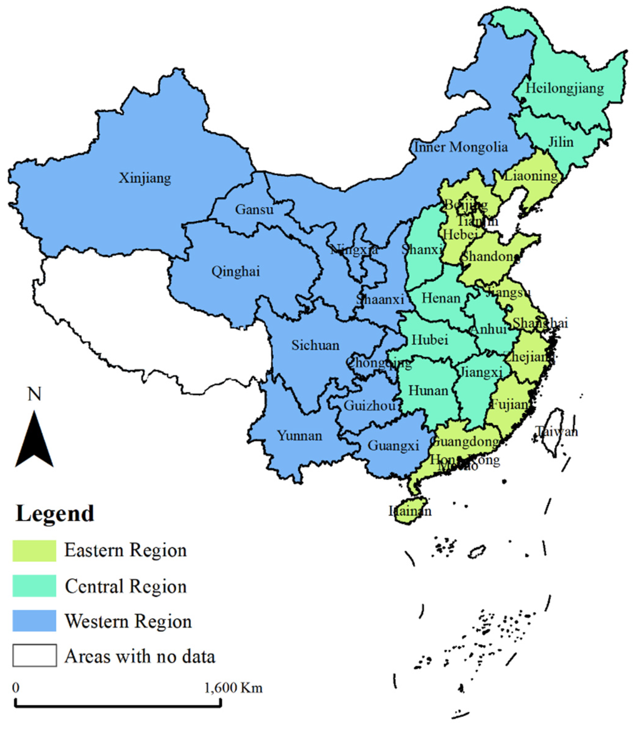
3.1. Spatial and Temporal Distribution of Urban and Rural Environmental Pollution

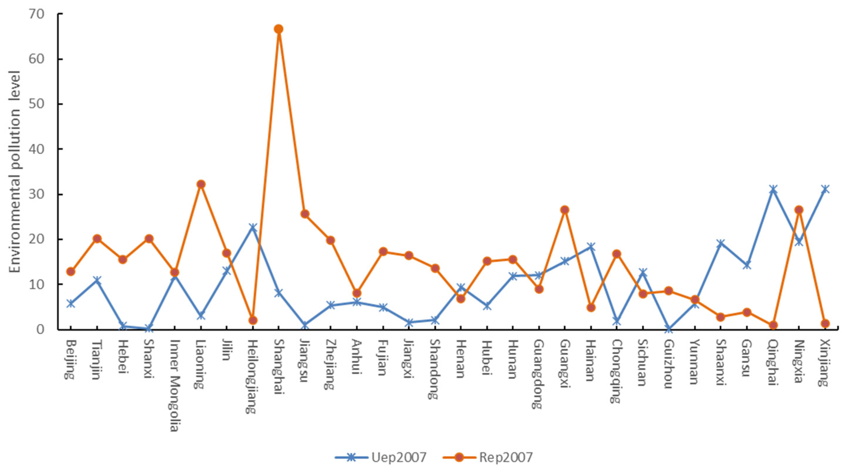
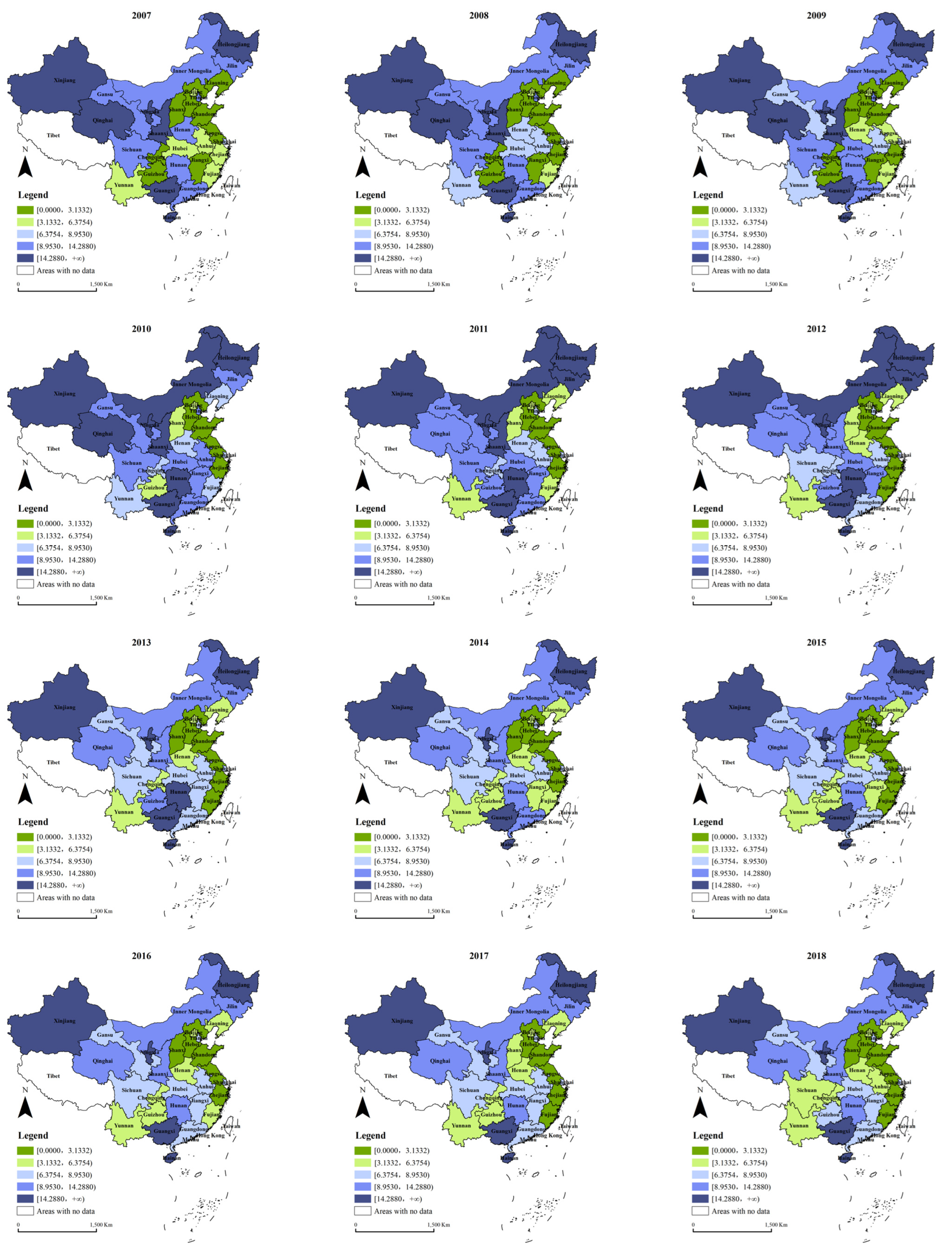
The average urban environmental pollution over the period from 2007 to 2022 stands at 9.0892. This value transitioned from 10.1574 in 2007 to 8.9540 in 2022, indicating an improvement over time. This metric serves as a foundational reference point for assessing the overarching trend in urban pollution levels (Figure 3).

Notably, 2010 stands out with the highest average pollution level at 11.6105, suggesting potentially elevated pollution during that year. Conversely, 2021 exhibits the lowest average pollution level at 7.6702, indicating a potential improvement or mitigation of pollution issues.

Examining individual years, 2010, 2011, 2007, 2008, and 2012 emerge as years with relatively high levels of urban environmental pollution. The proportion of years where urban environmental pollution exceeds the mean is 43.75%, indicating that less than half of the years during this period had pollution levels above the average. Conversely, 56.25% of the years had pollution levels below the mean.

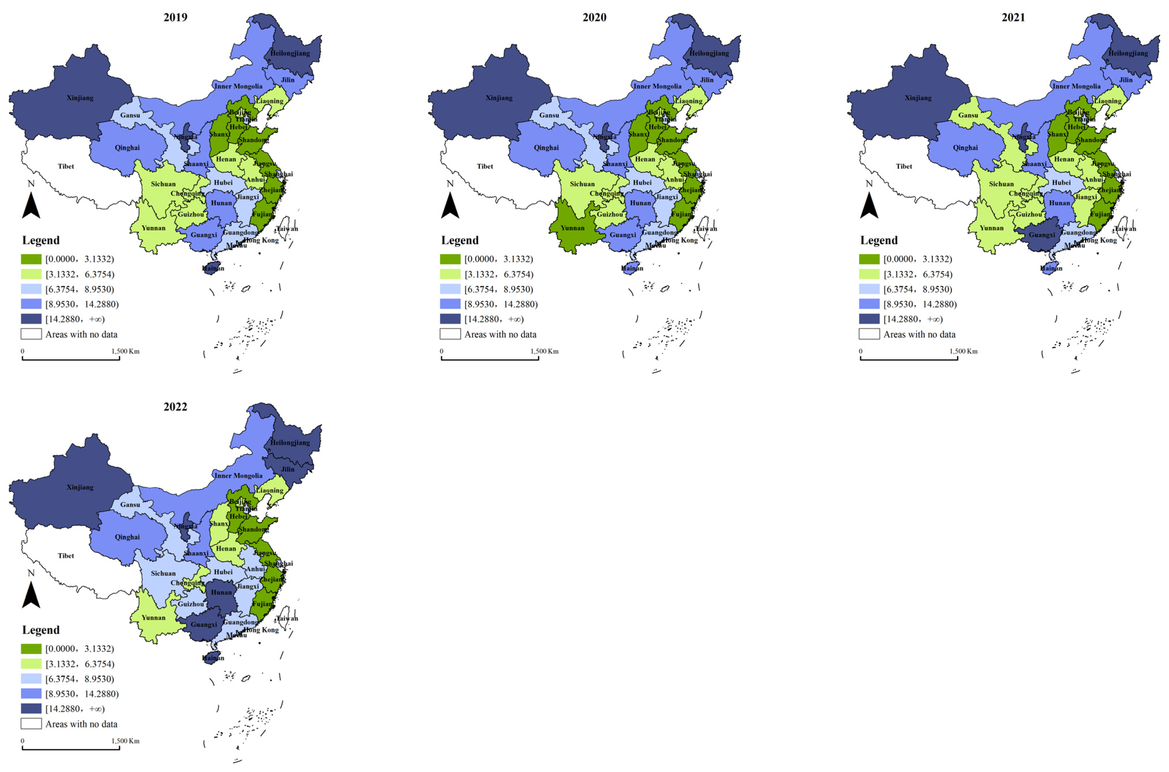
Conversely, 2021, 2020, 2019, 2018, and 2017 are identified as years with the smallest urban environmental pollution levels. This variability underscores the dynamic nature of urban pollution levels over time, with some years experiencing lower pollution levels compared to others.

Across the 30 provinces and municipalities studied, the average urban environmental pollution level aligns closely with the overall mean at 9.0892. Notably, Heilongjiang Province demonstrates the highest average pollution level, significantly exceeding the mean. Conversely, Hebei exhibits the lowest average pollution level among the provinces and municipalities studied.

Among the provinces and municipalities, Heilongjiang Province maintains the highest urban environmental pollution level, followed by Xinjiang, Guangxi, Ningxia, and Hainan. However, it is noteworthy that despite Heilongjiang’s high pollution level, the majority of provinces (63.33%) have mean values below the overall mean, indicating significant regional variation in pollution levels.

Conversely, Hebei stands out with the lowest urban environmental pollution level among the 30 provinces and municipalities, followed by Zhejiang, Jiangsu, Shandong, and Shanxi. These provinces may have implemented effective pollution control measures or possess favorable environmental conditions, contributing to their lower pollution levels compared to others.

From 2007 to 2022, the average level of rural environmental pollution stands at 14.8442, serving as a baseline for comprehending the broader trend in rural pollution levels. This value transitioned from 15.1123 in 2007 to 14.2675 in 2022, suggesting an improvement in performance over the specified timeframe. The year 2021 stands out with the highest average pollution level at 17.4535, indicating a potential peak in pollution during that year. Conversely, 2010 exhibits the lowest average pollution level at 11.7208, suggesting a relatively cleaner period (Figure 4).

Examining individual years, 2021, 2020, 2019, 2018, and 2017 emerge as years with relatively high levels of rural environmental pollution. The proportion of years where rural environmental pollution exceeds the mean is 56.25%, indicating that more than half of the years during this period had pollution levels above the average. Conversely, 43.75% of the years had pollution levels below the mean.

Conversely, 2010, 2011, 2009, 2012, and 2022 are identified as years with the smallest rural environmental pollution levels. This variability underscores the dynamic nature of rural pollution levels over time, with some years experiencing lower pollution levels compared to others.

Across the 30 provinces and municipalities studied, the average rural environmental pollution level aligns closely with the overall mean, at 14.8442. Notably, Shanghai demonstrates the highest average pollution level, significantly exceeding the mean. Conversely, Qinghai exhibits the lowest average pollution level among the provinces and municipalities studied.

Among the provinces and municipalities, Shanghai maintains the highest rural environmental pollution level, followed by Liaoning, Jiangsu, Zhejiang, and Tianjin. However, it is important to note that despite Shanghai’s high pollution level, the majority of provinces (56.67%) have mean values below the overall mean, indicating significant regional variation in pollution levels.

Conversely, Qinghai stands out with the lowest rural environmental pollution level among the 30 provinces and municipalities, followed by Xinjiang, Shaanxi, Gansu, and Hainan. These provinces may have implemented effective pollution control measures or possess favorable environmental conditions, contributing to their lower pollution levels compared to others.

3.2. Spatial Dependence of Urban and Rural Environmental Pollution

In summary,

Table 2. Global Moran index of urban environmental pollution and rural environmental pollution in China from 2007 to 2022.

Year	Uep			Rep
	Moran’s I	Z Value	p Value	Moran’s I	Z Value	p Value
Mean	0.189	2.432	0.008	0.190	2.483	0.007
2007	0.122	1.695	0.045	0.107	1.551	0.060
2008	0.110	1.564	0.059	0.154	2.079	0.019
2009	0.087	1.315	0.094	0.198	2.582	0.005
2010	0.170	2.271	0.012	0.247	3.139	0.001
2011	0.219	2.807	0.003	0.262	3.264	0.001
2012	0.173	2.272	0.012	0.172	2.261	0.012
2013	0.200	2.558	0.005	0.181	2.380	0.009
2014	0.203	2.582	0.005	0.173	2.303	0.011
2015	0.194	2.502	0.006	0.175	2.323	0.010
2016	0.193	2.486	0.006	0.188	2.472	0.007
2017	0.187	2.424	0.008	0.187	2.452	0.007
2018	0.183	2.378	0.009	0.179	2.361	0.009
2019	0.176	2.303	0.011	0.172	2.292	0.011
2020	0.176	2.304	0.011	0.172	2.290	0.011
2021	0.181	2.361	0.009	0.169	2.256	0.012
2022	0.196	2.525	0.006	0.185	2.440	0.007

indicates that (1) urban environmental pollution in the local area is positively correlated with that in neighboring urban areas, and that (2) rural environmental pollution in the local area is positively correlated with that in neighboring rural areas.

To further analyze the specific characteristics of the spatial clustering of urban environmental pollution and rural environmental pollution in each region, this study utilized Stata 16.0 to generate scatter plots of spatial correlation indices for urban environmental pollution and rural environmental pollution (Figure 5 and Figure 6).

3.3. Relationship Between Environmental Regulation and Environmental Pollution (Urban and Rural)

The baseline regression results, as summarized in

Table 3. Estimated results of environmental regulations on urban and rural environmental pollution.

Variables	Uep		Rep
	Regression Coefficients	Regression Coefficients	Regression Coefficients	Regression Coefficients
	(1)	(2)	(3)	(4)
lnEr	−1.293 ***	−1.144 ***	0.457 ***	0.508 ***
	(0.105)	(0.173)	(0.110)	(0.153)
lntran		0.132 *		−0.238 ***
		(0.076)		(0.068)
lnfin		−5.917 ***		8.159 ***
		(1.952)		(1.713)
lneci		0.055		0.195 **
		(0.095)		(0.083)
lnmar		−0.699 ***		2.597 ***
		(0.225)		(0.202)
lnpop		−0.446 ***		−0.109
		(0.089)		(0.079)
W × lnEr	0.005	1.915 ***	0.853 ***	1.565 ***
	(0.321)	(0.462)	(0.312)	(0.406)
W × lntran		0.296		0.692 ***
		(0.205)		(0.183)
W × lnfin		−21.205 ***		−10.679 ***
		(4.517)		(3.971)
W × lneci		−2.357 ***		−0.573***
		(0.259)		(0.218)
W × lnmar		1.225 **		0.162
		(0.620)		(0.607)
W × lnpop		0.386		−0.200
		(0.251)		(0.221)
ρ	0.369 ***	0.302 ***	0.388 ***	0.286 ***
	(0.075)	(0.100)	(0.072)	(0.098)
R2	0.254	0.247	0.140	0.573
Time	Yes	Yes	Yes	Yes
N	480	480	480	480

Note: The data in brackets are standard errors, and *, **, and *** indicate 10%, 5%, and 1% levels, respectively.

, lead to the following main conclusions. Higher levels of urban and rural environmental pollution in the local area are associated with higher levels of urban and rural environmental pollution in neighboring areas. This is evident from the coefficient ρ, where the coefficients for urban pollution (ρ = 0.302***) and rural pollution (ρ = 0.286***) both indicate positive associations.

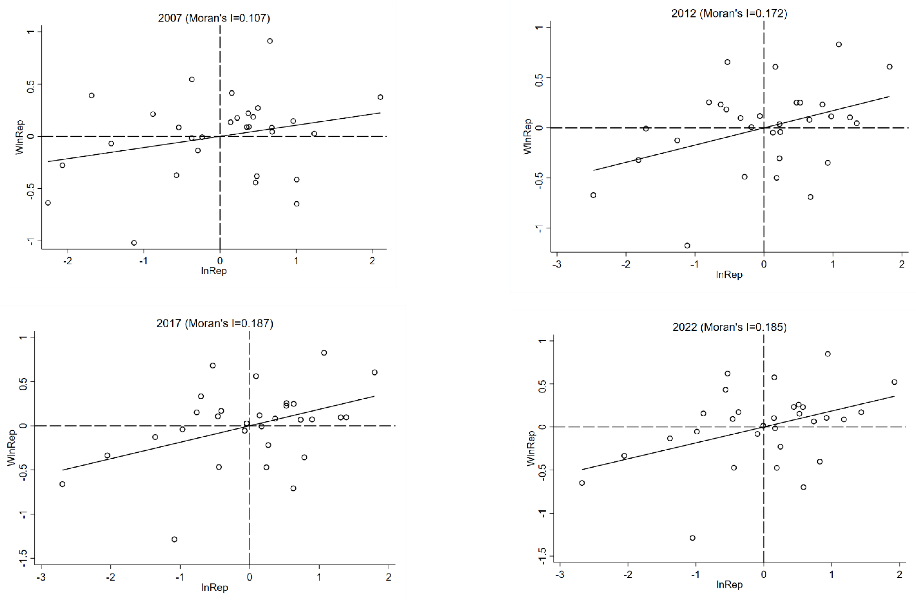
The spatial econometric regression results, as shown in columns (1) to (4) of Table 3, reveal that the estimated coefficients (ρ) for the spatial lag terms of urban and rural environmental pollution are positive and statistically significant at the 1% level. This indicates that there exists a positive spatial correlation between urban and rural environmental pollution across different regions.

Moreover, it is important to note that spatial econometric models differ from traditional econometric models in that the regression coefficients no longer reflect the direct impact of independent variables on the dependent variable due to the presence of spatial effects. Instead, they serve as preliminary indicators of the effects of various variables. To explore the role of spatial effects further, the decomposition of spatial effects is conducted, as presented in

Table 4. Decomposition results of the effects of environmental regulations on urban and rural environmental pollution.

Variables	Uep			Rep
	Direct Effect	Indirect Effect	Total Effect	Direct Effect	Indirect Effect	Total Effect
lnEr	−1.245 ***	1.844 ***	0.599 *	0.446 ***	1.156 ***	1.603 ***
	(0.189)	(0.414)	(0.335)	(0.166)	(0.363)	(0.289)
lntran	0.113 *	0.194	0.307 **	−0.278 ***	0.611 ***	0.333 **
	(0.067)	(0.152)	(0.147)	(0.060)	(0.137)	(0.135)
lnfin	−4.806 **	−15.755 ***	−20.561 ***	8.937 ***	−10.631 ***	−1.694
	(2.174)	(3.389)	(2.937)	(1.888)	(2.954)	(2.491)
lneci	0.172 *	−1.948 ***	−1.776 ***	0.230 **	−0.529 ***	−0.299 **
	(0.103)	(0.221)	(0.172)	(0.092)	(0.194)	(0.149)
lnmar	−0.809 ***	1.265 **	0.456	2.582 ***	−0.412	2.170 ***
	(0.269)	(0.604)	(0.518)	(0.239)	(0.532)	(0.451)
lnpop	−0.463 ***	0.434 **	−0.030	−0.095	−0.127	−0.222
	(0.097)	(0.177)	(0.169)	(0.086)	(0.152)	(0.148)

Note: The data in brackets are standard errors, and *, **, and *** indicate 10%, 5%, and 1% levels, respectively.

.

In terms of urban environmental pollution, the analysis reveals several noteworthy associations.

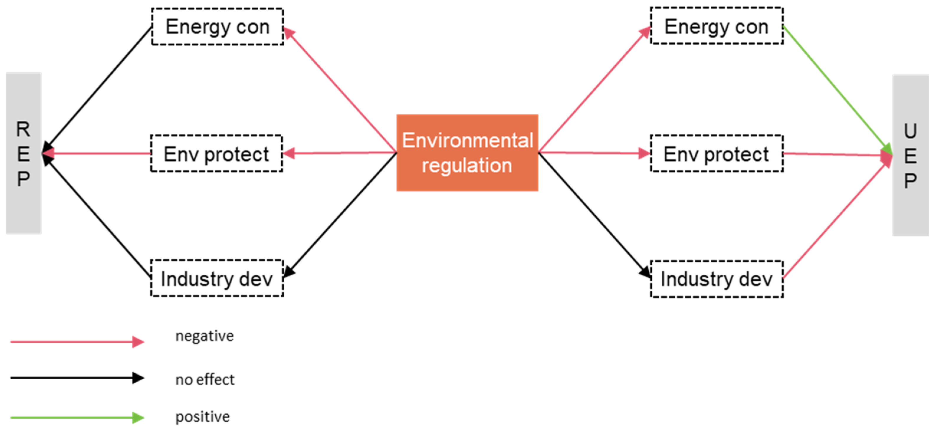
A decrease in the level of environmental regulation tends to lead to increased environmental pollution. In terms of the direct effect, a 1% increase in local environmental regulation results in a 1.245% increase in local environmental pollution (conversely, a 1% decrease in local environmental regulation leads to a 1.245% reduction in urban environmental pollution). This may be because when environmental regulation becomes less stringent, local enterprises in urban areas face fewer interventions and restrictions, allowing them greater flexibility and autonomy. As a result, while pursuing profits, these enterprises may also be more likely to reduce their negative impact on the environment.

In terms of the indirect effect, a 1% increase in environmental regulation in neighboring regions leads to a 1.844% increase in local urban environmental pollution (conversely, a 1% decrease in regulation in neighboring areas results in a 1.844% reduction in local urban pollution).

As for the total effect, a 1% increase in environmental regulation results in a 0.599% reduction in urban environmental pollution.

For each 1% increase in local transportation capacity, there is a concurrent 0.113% (0.113*) rise in local urban environmental pollution. However, the transportation capacity of neighboring areas shows no significant effect on local urban environmental pollution (0.194). Overall, a 1% increase in combined transportation capacity leads to a 0.307% (0.307**) rise in local urban environmental pollution. A 1% increase in local financial level corresponds to a substantial decrease of 4.806% (−4.806**) in local urban environmental pollution. Similarly, for every 1% increase in neighboring financial levels, there is a decrease of 15.755% (−15.755***) in local urban environmental pollution. Overall, a 1% increase in combined financial levels results in a remarkable decrease of 20.561% (−20.561***) in local urban environmental pollution.

An increase of 1% in local energy consumption intensity leads to a corresponding 0.172% rise (0.172*) in local urban environmental pollution. Conversely, for every 1% increase in neighboring energy consumption intensity, there is a significant decrease of 1.948% (−1.948***) in local urban environmental pollution. Overall, a 1% increase in combined energy consumption intensity results in a notable decrease of 1.776% (−1.776***) in local urban environmental pollution. With a 1% increase in local marketization level, there is a corresponding decrease of 0.809% (−0.809***) in local urban environmental pollution. However, a 1% increase in neighboring marketization levels leads to a contrasting increase of 1.265% (1.265**) in local urban environmental pollution. Notably, the marketization level of combined areas shows no discernible effect on local urban environmental pollution (0.456).

Local population size demonstrates a negative impact on local urban environmental pollution (−0.463***), indicating that as the population size increases, pollution tends to decrease. Conversely, neighboring population size does not significantly influence local urban environmental pollution (−0.434**). Overall, the population size of combined areas shows minimal impact on local urban environmental pollution (−0.030).

With local rural environmental regulation levels decreasing, local rural environmental pollution levels correspondingly increase. Similarly, a decrease in neighboring environmental regulation levels leads to a notable increase in local rural environmental pollution levels. Regarding transportation capacity, each 1% increase in local transportation capacity correlates with a decrease of 0.278% (−0.278***) in local rural environmental pollution. However, for rises in neighboring transportation capacity, there is a corresponding increase in neighboring rural environmental pollution.

Regarding financial factors, increases in local financial level are associated with a considerable aggravation in local rural environmental pollution. Conversely, for increases in neighboring financial levels, there is a notable improvement in local rural environmental pollution. However, the financial level of combined areas shows no significant effect on local rural environmental pollution. Energy consumption intensity also plays a role, with a 1% increase in local energy consumption intensity corresponding to a 0.230% increase in local rural environmental pollution. On the other hand, with increases in neighboring energy consumption intensity, there is a decrease in local rural environmental pollution. Moreover, increasing combined marketization levels leads to local rural environmental pollution increases.

3.4. The Impacts of Environmental Regulation on Urban and Rural Environmental Pollution

Environmental protection investment acts as a pivotal factor through which environmental regulation curbs urban and rural environmental pollution emissions (Figure 7). Essentially, in instances of weak environmental regulation intensity, augmenting environmental protection investment can bolster the adverse impact of environmental regulation on urban environmental pollution emissions.

Similarly, the energy consumption structure serves as a vital mechanism for inhibiting urban environmental pollution emissions through environmental regulation, while energy consumption regulation does not present an impact on rural environmental pollution. More specifically, environmental regulation can mitigate the consumption of coal energy, thereby resulting in a decline in urban environmental pollution. Both energy consumption structure and environmental protection investment emerge as crucial mechanisms shaping the influence of environmental regulation on urban environmental pollution. Consequently, environmental regulation can mitigate urban environmental pollution emissions by diminishing coal energy consumption structure and fostering environmental protection investment.

As shown in

Table 5. Estimated paths of the impacts of environmental regulations on urban environmental pollution.

Effect	Variables	Ecs	Eie	Agg	Uep	Uep	Uep
		(1)	(2)	(3)	(4)	(5)	(6)
Direct effect	Er	−0.012	0.196 **	−0.047 **	−1.197 ***	−1.225 ***	−1.077 ***
		(0.022)	(0.098)	(0.022)	(0.181)	(0.180)	(0.179)
	Ecs				1.036 ***
					(0.308)
	Eie					−1.038 ***
						(0.069)
	Agg						0.186
							(0.337)
Indirect effect	Er	0.280 ***	0.420	0.020	2.102 ***	1.798 ***	1.703 ***
		(0.082)	(0.330)	(0.047)	(0.340)	(0.362)	(0.349)
	Ecs				2.677 ***
					(0.764)
	Eie					0.009
						(0.165)
	Agg						−3.662 ***
							(0.717)
Total effect	Er	0.267 ***	0.616 **	−0.027	0.905 ***	0.572 *	0.626 *
		(0.077)	(0.306)	(0.036)	(0.304)	(0.329)	(0.319)
	Ecs				3.713 ***
					(0.671)
	Eie					−1.029 ***
						(0.152)
	Agg						−3.476 ***
							(0.781)

Note: The data in brackets are standard errors, and *, **, and *** indicate 10%, 5%, and 1% levels, respectively.

and

Table 6. Estimated paths of the impacts of environmental regulations on rural environmental pollution.

Effect	Variables	Ecs	Eie	Agg	Rep	Rep	Rep
		(1)	(2)	(3)	(4)	(5)	(6)
Direct effect	Er	−0.012	0.196 **	−0.047 **	0.625 ***	0.509 ***	0.388 **
		(0.022)	(0.098)	(0.022)	(0.146)	(0.155)	(0.165)
	Ecs				2.829 ***
					(0.239)
	Eie					−0.747 ***
						(0.153)
	Agg						−0.207
							(0.303)
Indirect effect	Er	0.280 ***	0.420	0.020	0.834 **	1.122 ***	1.133 ***
		(0.082)	(0.330)	(0.047)	(0.333)	(0.337)	(0.307)
	Ecs				−3.620 ***
					(0.806)
	Eie					0.325 ***
						(0.059)
	Agg						1.157 *
							(0.658)
Total effect	Er	0.267 ***	0.616 **	−0.027	1.459 ***	1.631 ***	1.521 ***
		(0.077)	(0.306)	(0.036)	(0.330)	(0.320)	(0.281)
	Ecs				−0.791
					(0.789)
	Eie					−0.423 ***
						(0.147)
	Agg						0.950
							(0.697)

Note: The data in brackets are standard errors, and *, **, and *** indicate 10%, 5%, and 1% levels, respectively.

, energy consumption structure and environmental protection investment play pivotal roles in mediating the impacts of environmental regulation on both urban and rural environmental pollution. The presentation of both direct and indirect effects is intended to underscore the estimation results of the total effect.

4. Heterogeneity Analysis

Given the varying levels of endowment and economic development across regions, this study divides the sample into eastern, central, and western areas to analyze how environmental regulations impact pollution reduction in each.

The findings suggest that only in the western region do stronger environmental regulations significantly reduce urban pollution. The specific results are as follows. In the eastern region, the direct effect (−0.004), indirect effect (−0.522), and total effect (−0.527) of environmental regulation on urban pollution are not statistically significant. In the central region, stricter regulations are associated with an increase in urban pollution (1.280%). In contrast, in the western region, enhanced environmental regulations lead to a reduction in urban pollution (2.267%).

Furthermore, the results indicate that strengthening environmental regulations improves rural pollution across all three regions, with the most pronounced effect in the west. In the eastern region, improved regulations decrease rural pollution by 0.771%; in the central region, by 0.814%; and in the western region, by 3.135%.

Overall, the study highlights that the impact of environmental regulations varies significantly by region, with the western region showing the greatest benefits for both urban and rural pollution reduction (

Table 7. Decomposition results of the effects of environmental regulations on urban and rural environmental pollution in different regions.

Effect	Variables	Uep			Rep
		East	Central	West	East	Central	West
Direct effect	lnEr	−0.004	0.599 **	−0.952 **	−0.437 ***	0.669 ***	−0.554
		(0.153)	(0.246)	(0.444)	(0.163)	(0.184)	(0.388)
Indirect effect	lnEr	−0.522	−1.878 ***	3.219 ***	1.208 ***	0.145	3.688 ***
		(0.396)	(0.447)	(0.940)	(0.356)	(0.282)	(0.625)
Total effect	lnEr	−0.527	−1.280 ***	2.267 ***	0.771 **	0.814 ***	3.135 ***
		(0.398)	(0.374)	(0.856)	(0.338)	(0.161)	(0.509)

Note: The data in brackets are standard errors, **, and *** indicate 5%, and 1% levels, respectively.

).

5. Discussions and Implications

This research contributes to the growing body of literature on environmental pollution by exploring the complex dynamics of pollution disparities between rural and urban regions in China. By examining the socio-economic factors, industrial activities, and policy interventions that shape these environmental inequities, this study sheds light on both the progress made and the challenges that persist in addressing pollution across different regions.

One of the key findings is that while both urban and rural environmental pollution have improved over time, rural areas continue to face more severe pollution burdens. The average urban pollution level from 2007 to 2022 stands at 9.0892, showing a significant decline from 10.1574 in 2007 to 8.9540 in 2022. This downward trend reflects a positive outcome of urban environmental management efforts. However, the average rural pollution level remains considerably higher at 14.8442, despite a decrease from 15.1123 in 2007 to 14.2675 in 2022. These figures suggest that while rural pollution has improved, it continues to be more problematic than urban pollution, highlighting the need for more targeted interventions in rural areas.

The study also identifies key drivers of environmental pollution in both urban and rural regions. Energy consumption and environmental protection investments are found to be critical pathways through which environmental regulations impact urban pollution levels. In contrast, in rural areas, only environmental protection investment significantly influences pollution reduction. This suggests that rural areas may be more responsive to direct financial investments in environmental protection, while urban areas require a more multifaceted approach that also addresses energy consumption patterns.

A notable regional disparity emerges in the effectiveness of environmental regulations. In the western region, stronger environmental regulations lead to a significant reduction in both urban and rural pollution, indicating that this area benefits the most from stricter enforcement. However, the impact of regulations in the eastern and central regions is less pronounced, particularly in urban areas where environmental regulations do not yield significant reductions in pollution. This suggests that regional differences in economic development, industrial structure, and policy enforcement play a crucial role in shaping the effectiveness of environmental regulations.

The findings underscore the importance of region-specific policies in addressing environmental pollution. While environmental regulations appear to be effective in improving rural pollution across all regions, the western region stands out as the area where both urban and rural pollution are most positively impacted. Policymakers should consider this regional variability when designing environmental policies, ensuring that regulations are tailored to the specific socio-economic and industrial contexts of each region.

The findings of this research have several important implications for policymakers and stakeholders involved in environmental governance and sustainable development in China [46,47,48]. First, the study highlights the need for a differentiated approach to environmental regulation, one that accounts for the distinct pollution dynamics and socio-economic conditions in both rural and urban regions [49,50]. The disparity between rural and urban pollution levels—where rural pollution remains significantly higher—calls for increased attention and resources dedicated to rural environmental management [51,52]. Targeted investments in rural environmental protection, which were shown to be a critical factor in reducing pollution, should be a priority [39,40].

The regional variation in the effectiveness of environmental regulations underscores the importance of tailored policies [53]. The fact that only the western region shows significant reductions in urban pollution due to stricter regulations suggests that a one-size-fits-all approach to environmental policy may not be effective [54]. Policymakers need to consider the unique industrial, economic, and environmental challenges of each region when formulating regulations [55,56]. For instance, the eastern and central regions may require additional support mechanisms, such as technological innovation or enhanced monitoring systems, to ensure that environmental regulations can yield the desired results in urban areas [57].

Energy consumption emerged as a key driver of urban pollution, highlighting the need for policies that promote cleaner and more sustainable energy use in cities [58,59]. This implies that urban environmental management strategies should not only focus on regulatory frameworks, but also address the broader energy infrastructure and consumption patterns that contribute to pollution [21,22,23]. Investments in renewable energy, energy efficiency, and cleaner industrial practices are crucial to complement regulatory efforts in urban areas [36].

Finally, the pronounced success of environmental regulations in the western region suggests that valuable lessons can be drawn from this area’s experience and potentially applied to other parts of the country [44]. The western region, traditionally less developed compared to the eastern and central regions, has demonstrated notable improvements in environmental quality following the implementation of targeted regulatory measures. These successes may be attributed to a combination of factors, including strong government commitment, effective enforcement mechanisms, adaptation to local conditions, and perhaps the relatively lower industrial base, which made pollution control more manageable [55,56].

By studying the specific policies, enforcement strategies, and institutional frameworks that contributed to this success, policymakers can gain insights into which approaches are most effective under different economic and environmental contexts. Additionally, the western region may serve as a model for integrating environmental goals with regional development strategies, illustrating how sustainable growth can be achieved without compromising ecological integrity. Applying these lessons to other regions—particularly those still struggling with high pollution levels—could help optimize the design and implementation of environmental regulations on a national scale [2,3]. Strengthening enforcement mechanisms, increasing environmental protection investments, and tailoring regulations to regional characteristics could help replicate these successes [11]. The overall improvement in both urban and rural pollution levels from 2007 to 2022 is encouraging, but the continuous adaptation and refinement of policies will be necessary to sustain and accelerate these positive trends [16,17].

6. Conclusions

Addressing the inequities at the intersection of energy, environment, and industry is essential for achieving a just transition that benefits both rural and urban communities. While rural areas often struggle with economic dependence on carbon-intensive industries and inadequate energy infrastructure, urban regions face challenges related to pollution, energy affordability, and environmental justice. This study sheds light on the energy–environment–industry nexus and rural–urban inequities in the context of a just transition, but several limitations remain. Data availability at the rural level is often limited or inconsistent, and the temporal scope may not capture long-term effects. Establishing causality is challenging due to overlapping socio-economic factors, and regional policy differences limit generalizability. The roles of technological innovation and informal sectors are also underexplored. Future research should employ more granular spatial data, longitudinal analysis, and integrated models, while incorporating stakeholder perspectives and focusing on justice and inclusion. Exploring green technology adoption and sustainable industrial strategies in rural areas will also be key to informing equitable and effective transition pathways.

References

1. Zhao, J.; Zhao, Z.; Zhang, H. The impact of growth, energy and financial development on environmental pollution in China: New evidence from a spatial econometric analysis. Energy Econ. 2021, 93, 104506. [Google Scholar] [CrossRef]
2. Bian, Y.; Song, K.; Bai, J. Impact of Chinese market segmentation on regional collaborative governance of environmental pollution: A new approach to complex system theory. Growth Change 2021, 52, 283–309. [Google Scholar] [CrossRef]
3. Liang, L.; Wang, Z.; Li, J. The effect of urbanization on environmental pollution in rapidly developing urban agglomerations. J. Clean. Prod. 2019, 237, 117649. [Google Scholar] [CrossRef]
4. Chen, X.; Chen, M. Energy, environment and industry: Instrumental approaches for environmental regulation on energy efficiency. Environ. Impact Assess. Rev. 2024, 105, 107439. [Google Scholar] [CrossRef]
5. Zhao, L.; Shao, K.; Ye, J. The impact of fiscal decentralization on environmental pollution and the transmission mechanism based on promotion incentive perspective. Environ. Sci. Pollut. Res. 2022, 29, 86634–86650. [Google Scholar] [CrossRef]
6. Adu, D.T.; Denkyirah, E.K. Economic growth and environmental pollution in West Africa: Testing the Environmental Kuznets Curve hypothesis. Kasetsart J. Soc. Sci. 2018, 40, 281–288. [Google Scholar] [CrossRef]
7. Bi, G.-B.; Song, W.; Zhou, P.; Liang, L. Does environmental regulation affect energy efficiency in China’s thermal power generation? Empirical evidence from a slacks-based DEA model. Energy Policy 2014, 66, 537–546. [Google Scholar] [CrossRef]
8. Danish Ulucak, R.; Baloch, M.A. An empirical approach to the nexus between natural resources and environmental pollution: Do economic policy and environmental-related technologies make any difference? Resour. Policy 2023, 81, 103361. [Google Scholar] [CrossRef]
9. Feng, Y.; Wang, X.; Liang, Z. How does environmental information disclosure affect economic development and haze pollution in Chinese cities? The mediating role of green technology innovation. Sci. Total Environ. 2021, 775, 145811. [Google Scholar] [CrossRef]
10. Guo, R.; Yuan, Y. Different types of environmental regulations and heterogeneous influence on energy efficiency in the industrial sector: Evidence from Chinese provincial data. Energy Policy 2020, 145, 111747. [Google Scholar] [CrossRef]
11. Hao, Y.; Zheng, S.; Zhao, M.; Wu, H.; Guo, Y.; Li, Y. Reexamining the relationships among urbanization, industrial structure, and environmental pollution in China—New evidence using the dynamic threshold panel model. Energy Rep. 2020, 6, 28–39. [Google Scholar] [CrossRef]
12. Zhou, X.; Feng, C. The impact of environmental regulation on fossil energy consumption in China: Direct and indirect effects. J. Clean. Prod. 2017, 142, 3174–3183. [Google Scholar] [CrossRef]
13. Liang, W.; Yang, M. Urbanization, economic growth and environmental pollution: Evidence from China. Sustain. Comput. Inform. Syst. 2019, 21, 1–9. [Google Scholar] [CrossRef]
14. Lin, B.; Zhang, A. Can government environmental regulation promote low-carbon development in heavy polluting industries? Evidence from China’s new environmental protection law. Environ. Impact Assess. Rev. 2023, 99, 106991. [Google Scholar] [CrossRef]
15. Zou, Y.; Wang, M. Does environmental regulation improve energy transition performance in China? Environ. Impact Assess. Rev. 2024, 104, 107335. [Google Scholar] [CrossRef]
16. Hassan, S.T.; Danish Khan, S.U.-D.; Xia, E.; Fatima, H. Role of institutions in correcting environmental pollution: An empirical investigation. Sustain. Cities Soc. 2020, 53, 101901. [Google Scholar] [CrossRef]
17. Hussain, M.; Dogan, E. The role of institutional quality and environment-related technologies in environmental degradation for BRICS. J. Clean. Prod. 2021, 304, 127059. [Google Scholar] [CrossRef]
18. Jiang, T.; Zhang, R.; Zhang, F.; Shi, G.; Wang, C. Assessing provincial coal reliance for just low-carbon transition in China. Environ. Impact Assess. Rev. 2023, 102, 107198. [Google Scholar] [CrossRef]
19. Li, K.; Fang, L.; He, L. How population and energy price affect China’s environmental pollution? Energy Policy 2019, 129, 386–396. [Google Scholar] [CrossRef]
20. Dong, F.; Wang, Y.; Zheng, L.; Li, J.; Xie, S. Can industrial agglomeration promote pollution agglomeration? Evidence from China. J. Clean. Prod. 2020, 246, 118960. [Google Scholar] [CrossRef]
21. Dong, Y.; Zhang, Y.; Liu, S. The impacts and instruments of energy transition regulations on environmental pollution. Environ. Impact Assess. Rev. 2024, 105, 107448. [Google Scholar] [CrossRef]
22. Feng, T.; Du, H.; Lin, Z.; Zuo, J. Spatial spillover effects of environmental regulations on air pollution: Evidence from urban agglomerations in China. J. Environ. Manag. 2020, 272, 110998. [Google Scholar] [CrossRef] [PubMed]
23. Manisalidis, I.; Stavropoulou, E.; Stavropoulos, A.; Bezirtzoglou, E. Environmental and Health Impacts of Air Pollution: A Review. Front. Public Health 2020, 8, 14. [Google Scholar] [CrossRef] [PubMed]
24. Liu, K.; Lin, B. Research on influencing factors of environmental pollution in China: A spatial econometric analysis. J. Clean. Prod. 2019, 206, 356–364. [Google Scholar] [CrossRef]
25. Liu, L.; Li, L. Effects of fiscal decentralisation on the environment: New evidence from China. Environ. Sci. Pollut. Res. 2019, 26, 36878–36886. [Google Scholar] [CrossRef]
26. Long, C.; Jiang, Z.; Shangguan, J.; Qing, T.; Zhang, P.; Feng, B. Applications of carbon dots in environmental pollution control: A review. Chem. Eng. J. 2021, 406, 126848. [Google Scholar] [CrossRef]
27. Mandal, S.K. Do undesirable output and environmental regulation matter in energy efficiency analysis? Evidence from Indian Cement Industry. Energy Policy 2010, 38, 6076–6083. [Google Scholar] [CrossRef]
28. Miao, C.; Meng, X.; Duan, M.; Wu, X. Energy consumption, environmental pollution, and technological innovation efficiency: Taking industrial enterprises in China as empirical analysis object. Environ. Sci. Pollut. Res. 2020, 27, 34147–34157. [Google Scholar] [CrossRef]
29. Neves, S.A.; Marques, A.C.; Patrício, M. Determinants of CO2 emissions in European Union countries: Does environmental regulation reduce environmental pollution? Econ. Anal. Policy 2020, 68, 114–125. [Google Scholar] [CrossRef]
30. Ouyang, X.; Li, Q.; Du, K. How does environmental regulation promote technological innovations in the industrial sector? Evidence from Chinese provincial panel data. Energy Policy 2020, 139, 111310. [Google Scholar] [CrossRef]
31. Pan, X.; Ai, B.; Li, C.; Pan, X.; Yan, Y. Dynamic relationship among environmental regulation, technological innovation and energy efficiency based on large scale provincial panel data in China. Technol. Forecast. Soc. Change 2019, 144, 428–435. [Google Scholar] [CrossRef]
32. Zhou, X.; Strezov, V.; Jiang, Y.; Kan, T.; Evans, T. Temporal and spatial variations of air pollution across China from 2015 to 2018. J. Environ. Sci. 2022, 112, 161–169. [Google Scholar] [CrossRef] [PubMed]
33. Pei, Y.; Zhu, Y.; Liu, S.; Wang, X.; Cao, J. Environmental regulation and carbon emission: The mediation effect of technical efficiency. J. Clean. Prod. 2019, 236, 117599. [Google Scholar] [CrossRef]
34. Wang, Y.; Deng, X.; Zhang, H.; Liu, Y.; Yue, T.; Liu, G. Energy endowment, environmental regulation, and energy efficiency: Evidence from China. Technol. Forecast. Soc. Change 2022, 177, 121528. [Google Scholar] [CrossRef]
35. Qi, X.; Sun, L.; Hu, Z.; Li, E.; Ning, Z. An applied framework to assess sustainability awareness and corporate misconduct considering just transition. Environ. Impact Assess. Rev. 2023, 103, 107261. [Google Scholar] [CrossRef]
36. Liu, Y.; Li, Z.; Yin, X. Environmental regulation, technological innovation and energy consumption—A cross-region analysis in China. J. Clean. Prod. 2018, 203, 885–897. [Google Scholar] [CrossRef]
37. Rahman, M.M.; Alam, K. Clean energy, population density, urbanization and environmental pollution nexus: Evidence from Bangladesh. Renew. Energy 2021, 172, 1063–1072. [Google Scholar] [CrossRef]
38. Wang, Z.; Feng, C. The impact and economic cost of environmental regulation on energy utilization in China. Appl. Econ. 2014, 46, 3362–3376. [Google Scholar] [CrossRef]
39. Siciliano, G.; Wallbott, L.; Urban, F.; Dang, A.N.; Lederer, M. Low-carbon energy, sustainable development, and justice: Towards a just energy transition for the society and the environment. Sustain. Dev. 2021, 29, 1049–1061. [Google Scholar] [CrossRef]
40. Liu, X.; Sun, T.; Feng, Q.; Zhang, D. Dynamic environmental regulation threshold effect of technical progress on China’s environmental pollution. J. Clean. Prod. 2020, 272, 122780. [Google Scholar] [CrossRef]
41. Ukaogo, P.O.; Ewuzie, U.; Onwuka, C.V. Environmental pollution: Causes, effects, and the remedies. In Microorganisms for Sustainable Environment and Health; Elsevier: Amsterdam, The Netherlands, 2020; pp. 419–429. [Google Scholar] [CrossRef]
42. Wang, C.; Wang, J.; Ai, W. Do urbanization, environmental regulation and GDP affect agricultural land use efficiency? Implications for just transition. Environ. Impact Assess. Rev. 2024, 105, 107421. [Google Scholar] [CrossRef]
43. Wu, H.; Hao, Y.; Ren, S. How do environmental regulation and environmental decentralization affect green total factor energy efficiency: Evidence from China. Energy Econ. 2020, 91, 104880. [Google Scholar] [CrossRef]
44. Zhang, Y.; Song, Y. Environmental regulations, energy and environment efficiency of China’s metal industries: A provincial panel data analysis. J. Clean. Prod. 2021, 280, 124437. [Google Scholar] [CrossRef]
45. Wu, H.; Li, Y.; Hao, Y.; Ren, S.; Zhang, P. Environmental decentralization, local government competition, and regional green development: Evidence from China. Sci. Total Environ. 2020, 708, 135085. [Google Scholar] [CrossRef]
46. Zhang, M.; Sun, X.; Wang, W. Study on the effect of environmental regulations and industrial structure on haze pollution in China from the dual perspective of independence and linkage. J. Clean. Prod. 2020, 256, 120748. [Google Scholar] [CrossRef]
47. Wu, H.; Xu, L.; Ren, S.; Hao, Y.; Yan, G. How do energy consumption and environmental regulation affect carbon emissions in China? New evidence from a dynamic threshold panel model. Resour. Policy 2020, 67, 101678. [Google Scholar] [CrossRef]
48. Yang, X.; Lin, S.; Li, Y.; He, M. Can high-speed rail reduce environmental pollution? Evidence from China. J. Clean. Prod. 2019, 239, 118135. [Google Scholar] [CrossRef]
49. Wu, R.; Lin, B. Environmental regulation and its influence on energy-environmental performance: Evidence on the Porter Hypothesis from China’s iron and steel industry. Resour. Conserv. Recycl. 2022, 176, 105954. [Google Scholar] [CrossRef]
50. Xu, B.; Xu, R. Assessing the role of environmental regulations in improving energy efficiency and reducing CO2 emissions: Evidence from the logistics industry. Environ. Impact Assess. Rev. 2022, 96, 106831. [Google Scholar] [CrossRef]
51. Yang, S.; Jahanger, A.; Hossain, M.R. How effective has the low-carbon city pilot policy been as an environmental intervention in curbing pollution? Evidence from Chinese industrial enterprises. Energy Econ. 2023, 118, 106523. [Google Scholar] [CrossRef]
52. Zhao, X.; Yin, H.; Zhao, Y. Impact of environmental regulations on the efficiency and CO2 emissions of power plants in China. Appl. Energy 2015, 149, 238–247. [Google Scholar] [CrossRef]
53. Yuan, B.; Ren, S.; Chen, X. Can environmental regulation promote the coordinated development of economy and environment in China’s manufacturing industry?—A panel data analysis of 28 sub-sectors. J. Clean. Prod. 2017, 149, 11–24. [Google Scholar] [CrossRef]
54. Zandalinas, S.I.; Fritschi, F.B.; Mittler, R. Global Warming, Climate Change, and Environmental Pollution: Recipe for a Multifactorial Stress Combination Disaster. Trends Plant Sci. 2021, 26, 588–599. [Google Scholar] [CrossRef] [PubMed]
55. Wang, L.; Le, Q.; Peng, M.; Zeng, H.; Kong, L. Does central environmental protection inspection improve corporate environmental, social, and governance performance? Evidence from China. Bus. Strategy Environ. 2023, 32, 2962–2984. [Google Scholar] [CrossRef]
56. Zhang, Y.; Xiong, Y.; Li, F.; Cheng, J.; Yue, X. Environmental regulation, capital output and energy efficiency in China: An empirical research based on integrated energy prices. Energy Policy 2020, 146, 111826. [Google Scholar] [CrossRef]
57. Yin, J.; Zheng, M.; Chen, J. The effects of environmental regulation and technical progress on CO2 Kuznets curve: An evidence from China. Energy Policy 2015, 77, 97–108. [Google Scholar] [CrossRef]
58. Zhao, X.; Mahendru, M.; Ma, X.; Rao, A.; Shang, Y. Impacts of environmental regulations on green economic growth in China: New guidelines regarding renewable energy and energy efficiency. Renew. Energy 2022, 187, 728–742. [Google Scholar] [CrossRef]
59. Wang, X.; Zhang, R.; Jiang, T. Energy justice and decarbonization: A critical assessment for just energy transition in China. Environ. Impact Assess. Rev. 2024, 105, 107420. [Google Scholar] [CrossRef]
Figure 1. Research area.
Land 14 01161 g001
Figure 2. Urban and rural environmental pollution inequity. Note: above 2007; below 2022.
Land 14 01161 g002aLand 14 01161 g002b
Figure 3. Urban environmental pollution changes over the past 15 years.
Land 14 01161 g003aLand 14 01161 g003b
Figure 4. Rural environmental pollution changes over the past 15 years.
Land 14 01161 g004aLand 14 01161 g004b
Figure 5. Moran index scatter plot of urban environmental pollution.
Land 14 01161 g005
Figure 6. Moran index scatter plot of rural environmental pollution.
Land 14 01161 g006
Figure 7. Impacts of environmental regulation on urban and rural environmental pollution.
Land 14 01161 g007