A Novel Geospatial Approach for Analyzing Coastal Roadway Vulnerability to Shoreline Changes

Abstract

Climate changes and coastal development pose growing risks to coastal roadways constructed on flat and low-elevation terrains near retreating shorelines. Although GIS has been widely used for shoreline change analysis and roadway management, significant limitations remain in accurately analyzing shoreline changes relative to roadways and integrating the analysis results into roadway spatial databases in the Geographic Information System (GIS). In this regard, this study proposes a novel geospatial approach that integrates the linear referencing system (LRS) with the vector-offset based analysis method for shoreline change. The LRS, implemented in GIS, defines the specific positions of a roadway using relative distances from predefined referents. Vector offsets, representing the shortest distance and direction from historical shorelines to the roadway, are then employed to analyze shoreline changes. The proposed approach was applied to a coastal roadway experiencing significant shoreline changes driven by climate change and the construction of coastal infrastructure. The results demonstrate the effectiveness of the proposed approach in analyzing shoreline retreat caused by coastal infrastructure development, as well as shoreline accretion following the installation of erosion control structures. These results, which closely reflect the actual erosion pattern, indicate that the proposed approach can effectively support planning for roadway maintenance and reinforcement.

1. Introduction

A coastal region, which is the interface between land and ocean, is the central zone for economic and social activities, as a large portion of the global population resides near the coast [1]. This high population density has led to the substantial development of infrastructure to support human settlement, transportation, and urban development [2,3]. Coastal roadways are critical components of public infrastructures. These linear corridors are often aligned parallel to the shoreline to efficiently connect various coastal locations such as ports, residential zones, and recreation areas, and to serve as essential entry and evacuation routes during emergencies, including severe storms and tsunamis. However, coastal roadways are increasingly vulnerable to climate changes, including more severe storms and sea-level rise. In addition, anthropogenic activities such as land reclamation and construction have significantly altered coastal morphology and disrupted natural ecosystems [4,5,6]. Constructed along flat, low-elevation terrain to provide efficient access to beachfront areas and to minimize construction cost, coastal roadways near shorelines are highly susceptible to wave attack and sediment loss [7,8,9]. Shoreline recession progressively narrows the beach, reducing the natural buffer zone that protects the roadway from direct wave impact. The increased exposure, especially during storm surges, accelerates the deterioration of roadway pavements and adjacent structures such as bridges and culverts. Consequently, damage to the roadway can substantially disrupt local access and compromise infrastructure such as residential buildings, utility networks, and telecommunications systems [10,11,12].

The Geographic Information System (GIS) has been widely used to manage coastal roadway and support strategic planning for roadway reinforcement. For example, machine learning models combined with multi-temporal spatial and non-spatial datasets were applied in GIS to predict shoreline erosion patterns and short-term coastal evolution [13,14,15,16]. Composite vulnerability indices for assessing coastal roadways were formulated by integrating geomorphological factors and shoreline dynamics, enabling the systematic assessment of roadway susceptibility to storm impacts [8,11,17]. In addition, GIS-based tools were designed to evaluate roadways’ exposure to coastal erosion and to assist in identifying adaptation strategies for vulnerable coastal areas [18,19]. However, despite these efforts, limitations remains in accurately analyzing shoreline changes in relation to roadways. Integrating shoreline change analysis methods into GIS is essential to further enhance its capabilities for roadway management.

The shoreline is considered a temporal geographic feature as its position and shape are continuously reformed by a combination of natural processes and anthropogenic activities [20,21,22]. Shoreline advance and retreat reflect changes in coastal conditions such as fluvial sediment supply, tidal pattern, and relative sea level [23,24]. Numerous spatial analysis methods have been proposed to identify and analyze shoreline changes and their variabilities on diverse temporal and spatial scales [25,26,27,28,29,30,31]. Among these, two widely adopted approaches are the transect-based analysis (TBA) and the area-based analysis (ABA) methods [32]. Figure 1 conceptually illustrates how the TBA and ABA methods are applied for shoreline change analysis. The TBA method is based on the generation of transects orthogonal to the baseline. The transect distances between the baseline and shoreline are then measured to compute shoreline offsets (Figure 1a). The ABA method, also referred to as the change polygon method [33], computes a shoreline offset by dividing the beach area by the average length of the shoreline and baseline (Figure 1b). The use of the two methods depends on time, resources, and the extent of the area. The ABA method provides an overall assessment of shoreline erosion or accretion, whereas, the TAB method is effective for detailed analysis along short and specific sections of the beach [34].

The TBA and ABA methods can be easily implemented in GIS to evaluate shoreline changes concerning coastal roadways. However, several factors should be considered when the roadway servers as the baseline. A roadway centerline map consists of straight and curvilinear lines. For example, when a curvilinear roadway centerline serves as a baseline for the TBA method, transects from concave sections of the baseline may not reach the closest shoreline and may instead intersect each other (Figure 2a). Also, in Figure 2b, two shorelines should have identical mean offsets from the baseline. However, for the ABA method, the shoreline offset is subject to the complexity of shoreline shape, as greater complexity results in longer computed shoreline length, which, in turn, leads to inconsistent shoreline offsets. Therefore, an alternative method is required to consistently quantify shoreline change, regardless of the shapes of the roadway centerline and shoreline.

This study aims to integrate the shoreline change analysis method with GIS for coastal roadway management. However, most spatial data related to roadway assets and shorelines are spatially referenced using the two-dimensional (2D) geodetic coordinate system, which is incompatible with the one-dimensional (1D) domain of roadway spatial databases in GIS. These two disparate spatial reference systems impose complexity in managing roadways and analyzing their dynamic interactions with shoreline changes. In this regard, two objectives of this study are: (1) to present a shoreline change analysis method for accurately assessing and monitoring shoreline changes in relation to roadways, and (2) to design a geospatial reference framework that integrates the linear domain of roadways with information on roadway assets and their vulnerability to shoreline changes. The remainder of this paper is organized as follows: Section 2 conceptually describes the proposed approach for analyzing shoreline changes in relation to coastal roadways and adjacent assets, as well as its integration into GIS for enhanced shoreline change analysis and roadway management. In Section 3, a case study is presented to demonstrate the implementation of the proposed approach and to evaluate its applicability and effectiveness in a real-world coastal roadway. Finally, the discussion and conclusion are presented with future research in Section 4 and Section 5.

2. Methodology

2.1. Overview

The novel geospatial approach, proposed in this paper, implements the Linear Referencing System (LRS) into GIS as a geospatial reference framework for locating roadway assets and analyzing their offsets relative to shorelines. The LRS, which comprises a set of policies, records, procedures, and linear referencing methods [35], is used to standardize the referencing and management of spatial data along the linear domain of roadways. In GIS, LRS defines locations along the roadway using the relative distance from predefined referents rather than geographic coordinates, thereby enabling precise event mapping and spatial analysis within a linear domain of roadway networks. This approach consists of two major components: (1) the vector offset analysis (VOA) method for shoreline change, detailed in Section 2.2, and (2) the LRS-based linear referencing method combined with the VOA method, which identifies and analyzes historical shorelines in close proximity to roadways and its adjacent facilities, as described in the Section 2.3.

2.2. VOA Method for Shoreline Change Analysis

2.2.1. Statistical Properties of Vector Offset Along a Line

In this study, the VOA method is formulated by redefining the statistical and probabilistic basis of the discrete displacement analysis method [36], which is derived from the buffering-based method [37] for analyzing positional shift. The buffering-based method assumes that a buffer around a line represents a probabilistic region that follows a normal distribution. Similar to the discrete displacement analysis method, the proposed method assumes that a line is theoretically considered as a set of infinite number of points. A set of vector offsets from these points along the line is adopted as the analytical alternative to the traditional line buffer. For example, when a line segment, $p_1{p}_2$, is defined by two end points, ${p_1=[x_1,y_1]}^T$ and ${p_2=[x_2,y_2 ]}^T$, an arbitrary point ${p_t=[x_t,y_t ]}^T$ where $\mathrm{t}\in [0,1]$, is defined by

$$\begin{array}{c}{x}_t=\mathrm{t}{x}_1+\left(1-t\right)x_2\\ y_t=\mathrm{t}{y}_1+\left(1-t\right)y_2\end{array}$$

(1)

Each point is assumed to be independent and to have an identical error (referred to as a vector offset hereinafter) from its true position, which follows a 2D circular normal distribution. Accordingly, in Equation (2), the $x_t$ and $y_t$ components of each point $p_t$ have the vector offsets that are independent and identically distributed with a standard deviation ($\sigma )$.

$$f\left(x_t,y_t\right)={\displaystyle \frac{1}{2\pi {\sigma }^2}}exp\left\{{\displaystyle \frac{-1}{2}}\left[{\left({\displaystyle \frac{x-x_t}{\sigma }}\right)}^2+{\left({\displaystyle \frac{y-y_t}{\sigma }}\right)}^2\right]\right\}$$

(2)

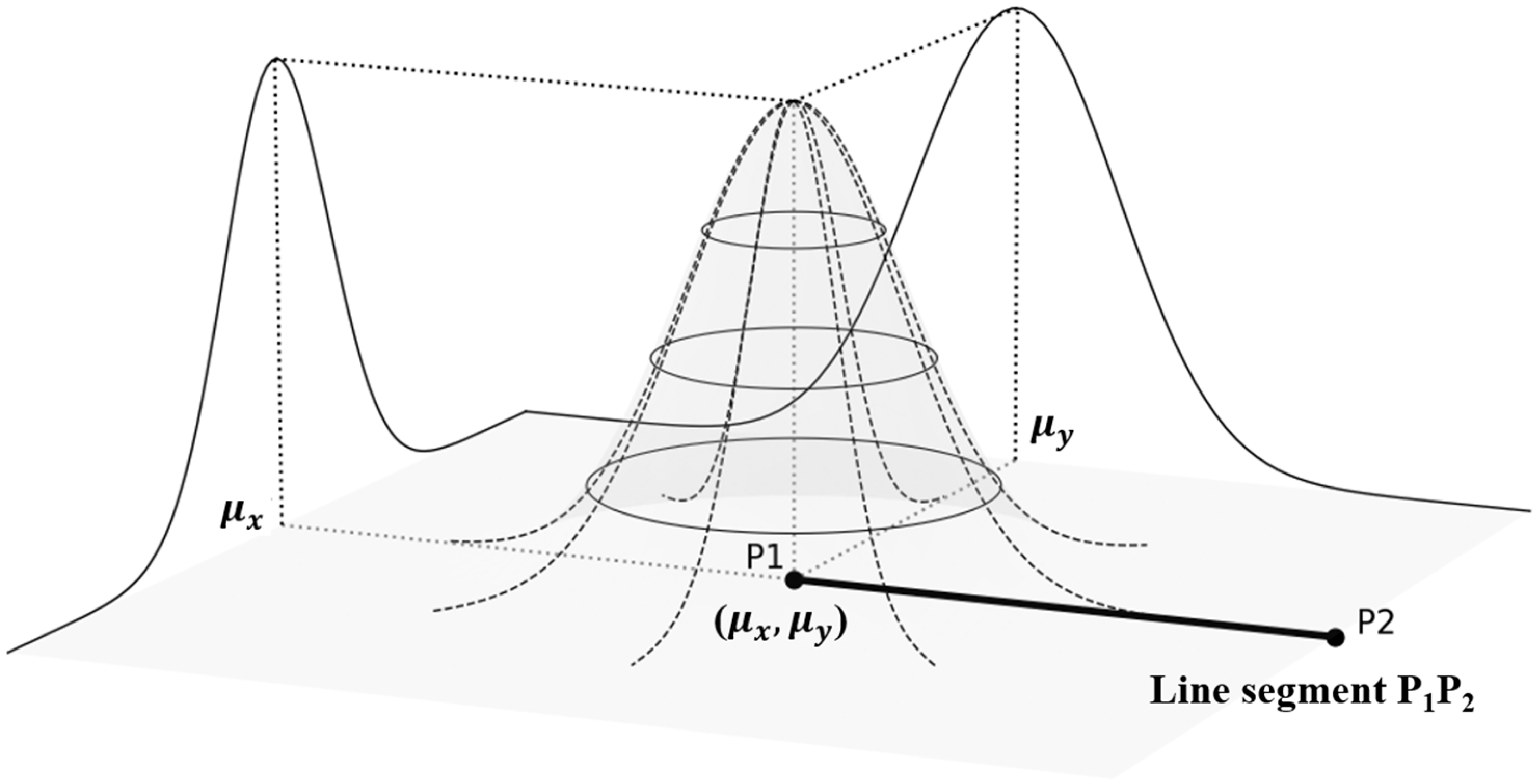
The distribution of the vector offset can be depicted using an error ellipse, $g\left(x_t,y_t,K\right)$, at the point, $p_t,$ create by setting the normal distribution, $f\left(x_t,y_t\right),$ equal to the height K of the intersecting plane above the x–y plane (Equation (3)). In Figure 3, each error ellipse at the end point $p_1$ represents a probabilistic region at a specified confidence level. Also, when they are projected onto the x–y plane, a multiple-ring buffer can be generated.

$${ g\left(x_t,y_t,K\right)=\left(x-x_t\right)}^2+{\left(y-y_t\right)}^2-{\ln \left[4{\pi }^2{{\sigma }^{4}K}^2 \right]}^{-1}{\sigma }^2=0$$

(3)

The line buffer around the line segment, $B_{p_1{p}_2,}$, is then constructed by a union of the error ellipses (${\cup }_{t=0}^{1}g\left(x_t,y_t,K\right))$ at $x_t$ and $y_t$ in Equation (4). In Figure 4, the line buffer has a constant width on either side of the line segment and its two end points. In the VOA method, vector offsets are generated along the line segment, conforming to the statistical properties of the buffering-based methods. The vector offset is the shortest distance from the center of an error ellipse to its boundary. The vector offsets at two endpoints radiate outward, conforming to the circular shape of the error ellipse, representing a 2D normal distribution, while the vector offset perpendicular to the line segment conforms to a set of 1D normal distributions. Therefore, the vector offset along the line segment has a complementary duality with the line buffer in Figure 4.

$$B_{p_1{p}_2}={\cup }_{t=0}^{1}g\left(x_t,y_t,K\right)$$

(4)

2.2.2. Application and Validation

In the VOA method, a set of vector offsets from a baseline is a major means of quantifying a positional shift to a target line (Figure 5). However, since a line is defined as a continuous feature composed of an infinite number of points, there is inherently an infinite number of possible distances measurements between the baseline (or true line) and the target line. Therefore, in the application, the procedure for vector offset analysis is as follows (Figure 5).

(1)

Sample points on the target line are determined at a predetermined interval, as defined in Equation (1).

(2)

For each sample point, a vector offset is generated from the nearest corresponding point on the baseline to the target line.

(3)

Each offset is assigned a positive or negative distance depending on its direction relative to the baseline.

(4)

The mean and standard deviation of all vector offsets are calculated to analyze a positional offset and the spatial variation between the baseline and the target line.

Figure 5 illustrates how the VOA method analyzes vector offsets depending on the spatial relationship between the baseline and the target line. Vector directions upward and downward relative to the baseline is defined as positive and negative offsets, respectively. Also, two target lines in Figure 5a,c are designed to be parallel and equidistant from the target line in Figure 5b. For all target lines, the mean offsets and standard deviations are calculated, using vector offsets generated from identical sample points along the baseline. In the analysis, the mean offset and its standard deviation represent the positional shift and its variability, respectively. For example, the mean offsets for the target lines in Figure 5a,c are −12.00 m and 12.00 m, indicating that their positional shifts are identical but opposite side relative to the baseline. Also, in Figure 5b, where the target line intersects the baseline, the positive and negative offsets are symmetrical to each other, resulting in the mean offset of 0.00 m. Despite differences in mean offsets, an identical standard deviation computed from all datasets indicates the spatial variability of the target lines remains consistent.

For validation purposes, the VOA method is experimentally compared and analyzed with the TBA method in Figure 6 and with the ABA method in Figure 7. Figure 6a shows the straight horizontal target line and the V-shaped baseline, to which the VOA and TBA methods are applied for positional offset analysis in Figure 6b and Figure 6c, respectively. In the VOA method, sample points are placed at 5-m intervals along the target line. Vector offsets are then generated from the closest points on the baseline, and the mean offset and standard deviation are calculated as 26.77 m and 3.44 m. In contrast, the TBA method generates perpendicular transects at 5-m intervals along the baseline, which results in intersecting transects and consequently leads to a significant overestimation of the mean offset, computed at 29.93 m.

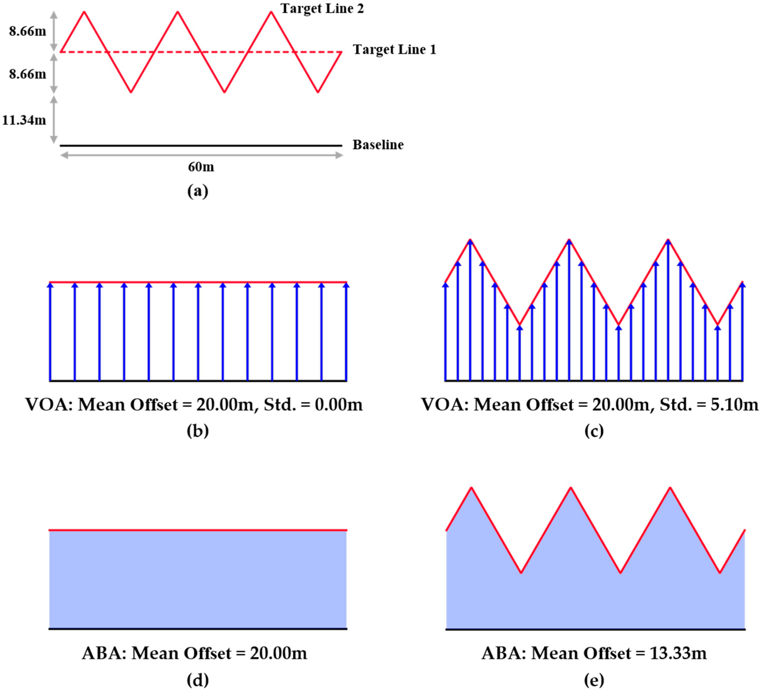
Also, in Figure 7a, the zigzag-shaped target line (Target Line 1) is designed with an amplitude of 8.66 m along the straight horizontal target line (Target Line 2). Positional offset from the straight baseline, which is parallel to Target Line 1, is analyzed using the VOA method in Figure 7b,c, and the ABA method in Figure 7d,e. The VOA method demonstrates that the mean offset is identical for both target lines. Additionally, the standard deviation for Target Line 1 is 0.00 m, while that for Target Line 2 is 5.10 m. In contrast, the ABA method computes the mean offset as 20.00 m for Target Line 1 but underestimates the mean offset for Target Line 2, calculating it as 13.33 m due to the increased length of the zigzag-shaped line. Overall experiment results indicate that the TBA and ABA methods are highly sensitive to the geometric configuration of the baseline and target line, leading to significant variations in offset estimation. In contrast, the VOA method demonstrated robust performance regardless of shape complexity or spatial variability, effectively overcoming the limitations of traditional shoreline change analysis methods. Furthermore, the VOA method enables quantitative assessment of spatial configuration between the baseline and target line through both mean offset and standard deviation analysis.

2.3. LRS-Based Linear Referencing with the VOA Method for Shoreline Change Analysis

2.3.1. LRS-Based Linear Referencing Method

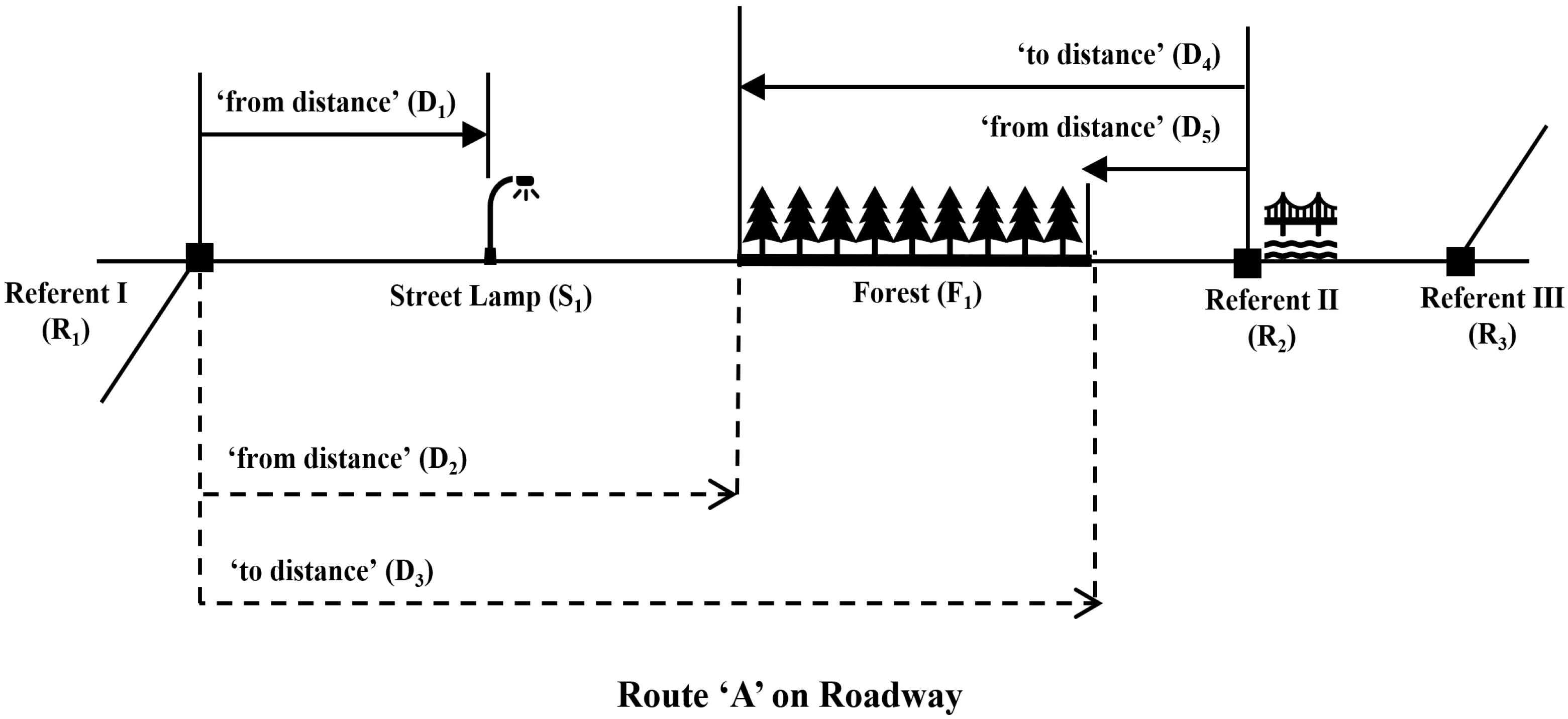
In the proposed approach, the LRS is adopted as a geospatial framework for recording and managing roadway facilities and its adjacent areas. The LRS is conceptually illustrated in Figure 8, where three referents are sequentially positioned along the route ‘A’. The referents have a relative distance from the start of a roadway. For example, the first referent (Referent I), located at the start of Route ‘A’, is assigned a certain value (R₁ = 0), while the third referent (Referent III) is assigned a value corresponding to the entire length of Route ‘A’ (R₃). Since the referent is a uniquely identified and known location along roadways, such as a street intersection or a bridge terminus, roadway assets of interest can be easily located and managed relative to the referents. For example, the location of the streetlamp (S₁) is linearly referenced with the ‘from distance’ (D₁) from the first referent (Referent I) as

$$S_1=R_1+D_1$$

(5)

Also, the spatial extent of the forest can be represented as a contiguous spatial interval along the roadway. Distance measures ‘from/to distances’ (D₅ and D₄, respectively) from the second referent (Referent II) are used to bound the forest (F₁). Since those measurements are made in the opposite direction of Route ‘A’, their values are negative. The forest (F₁) can also be defined using the distance measures ‘from/to distances’ (D₂ and D₃, respectively) from the first referent (Referent I). Consequently, the linear location of forest (F₁) can be expressed as relative distances from the second referent (Referent II) in Equation (6).

$${D_2=R}_2-D_4\le F_1 \le {D_3=R}_2-D_5$$

(6)

2.3.2. Integration of LRS-Based Linear Referencing with VOA Method in GIS

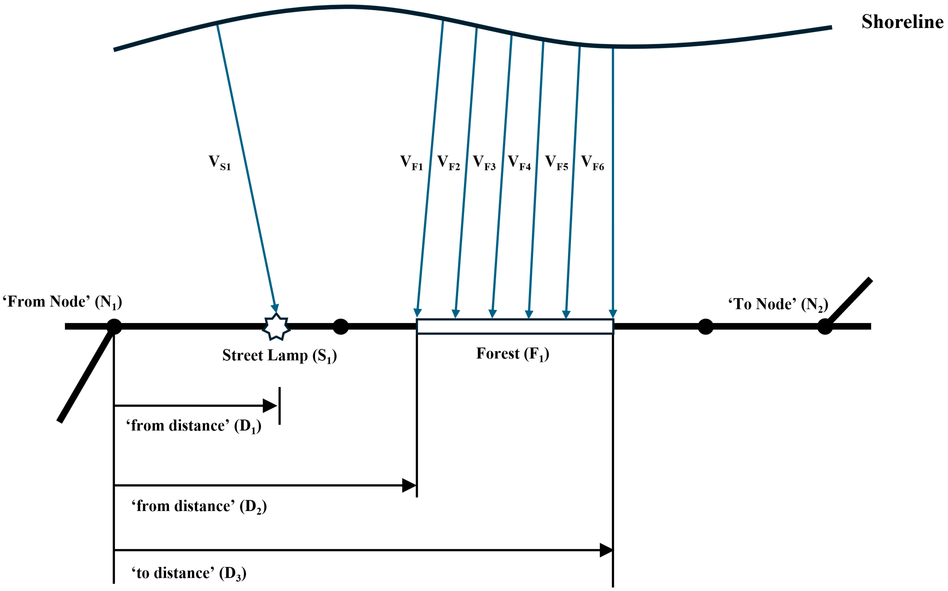
The LRS-based linear referencing method is implemented in the roadway network in GIS, where the referent is used to relate the real world to its corresponding locations in the GIS-based roadway network. For example, the ‘from node’ (N₁) and ‘to node’ (N₂) in Figure 9, which are identical to the first and third referents (Referents I and III) in Figure 8, provide the basis for locating the streetlamp as a point feature and the forest as linear features along the roadway network. However, a single roadway link, which stores homogeneous attributes, is unable to represent various features. The excessive segmentation of nodes and links increases network complexity and reduces maintenance efficiency. Thus, the dynamic segmentation combined with the event table is employed to create and manage the spatial representation of point and linear features temporarily, as needed. For example, in

Table 1. Point event table for the streetlamp.

Route ID	From Distance	Streetlamp ID	Offset
A	R1 + D1	S1	VS1

, the point event table for the streetlamp (S₁) within the roadway spatial database in GIS includes the key fields to define the route ID, the ‘from distance’ measure, and the asset-specific attributes. In

Table 2. Line event table for the forest.

Route ID	From Distance	To Distance	Land Use ID	Offset (Mean)	Offset (Std.)
A	R1 + D2	R1 + D3	F1	VF_mean	VF_std

, the key fields in the line event table for the forest (F₁) are similar to those in the point event table. However, the positions of a linear feature are defined using the values in the ‘from distance’ and the ‘to distance’ fields.

In the proposed approach, another major consideration is to analyze the shoreline changes with respect to roadway facilities and their adjacent land uses, for which the LRS-based linear referencing method is combined with the VOA method in Section 2.2. The shoreline change is analyzed with the premise that shorelines closer to the roadway have a greater impact on the roadway. The vector offset, which is the shortest distance from a shoreline to a roadway asset, is used not only for analyzing shoreline changes but also for identifying roadways and their surroundings at high risk of shoreline recession. In Figure 9, the LRS-based linear referencing method specifies the linear location of the streetlamp (S₁), to which the vector offset (V_S1) from a shoreline is created, and its distance is additionally recorded in Table 1. Also, a set of vector offsets from the shoreline is generated to evenly distribute points over the linear extent of the forest (F₁). The mean and standard deviation of the vector offsets, denoted as V_{F_mean} and V_{F_std}, are then calculated and recorded in Table 2.

3. Application and Results

3.1. Overview

The proposed approach is designed to analyze shoreline changes along coastal roadways and to identify roadway segments susceptible to shoreline erosion. The Maengbang coastal roadway in South Korea, experiencing significant shoreline changes due to climate change and anthropogenic development, was selected as the study area (Section 3.2). The LRS was first established as the geospatial framework for linearly locating the coastal roadway and its assets, and the LRS-based linear referencing with the VOA method was implemented in GIS for analyzing roadway vulnerability in response to shoreline changes (Section 3.3). Finally, the proposed approach was applied to shoreline data from 2018 to 2023, and its effectiveness is demonstrated through an analysis of shoreline changes impacting the roadway and its nearby assets (Section 3.4).

3.2. Study Area

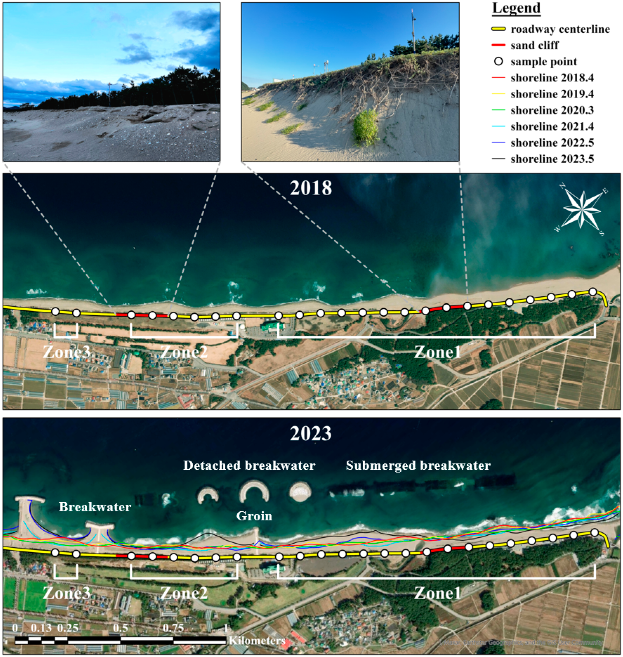
The Maengbang coastal roadway is located along the eastern coast of South Korea, with an adjacent sand beach extending approximately 4 km (37°23′15″–37°24′20″ N, 129°12′40″–129°14′10″ E). Due to its long stretch of beach and shallow coastal waters, Maengbang beach has become a prominent tourist destination, featuring various cultural and recreational facilities (e.g., resorts, camping sites, and golf courses) along the coastal roadway. However, the impacts of climate change (e.g., rising sea levels and an increased frequency of high waves and typhoons) have gradually reduced the beach width. In particular, shoreline erosion has accelerated since the construction of a thermal power plant and a coal unloading berth in 2018, resulting in a noticeable narrowing of the beach (Figure 10). As a consequence, in certain roadway sections, the distance between the shoreline and the roadway was decreased to less than 30 m, leading to the formation of sand cliffs and a marked increase in roadway collapse risk due to shoreline retreat. In response, the central government designated Maengbang beach as a shoreline erosion management zone to restrict development activities. A vegetated buffer zone was created along the roadway to mitigate damage caused by waves and wind. Furthermore, erosion control structures have been under construction since 2020, with completion targeted for 2025. Therefore, the continuous monitoring of shoreline changes and roadway assets management is essential to evaluate the effectiveness of these structures and to detect any new erosion potentially induced by their installation.

3.3. Implementation of LRS-Based Linear Referencing with VOA Method

In the LRS-based linear referencing method, a referent is a basis for determining linear locations along roadways. Referents must be unique and known locations to enable people to easily identify and record the locations of roadway assets and facilities. The Maengbang coastal roadway is a straight roadway along the shoreline, intersecting with other roadways for local access (Figure 11a). Also, some of the streetlamps installed at regular intervals are assigned unique identification numbers (IDs) and designated as report spots, allowing for the efficient location identification and incident reporting in the event of criminal, traffic, or maritime emergencies (Figure 11b). Therefore, in this study, roadway intersections and reporting spots are designated as referents to determine specific positions of erosion-susceptible sections (e.g., sand cliffs) and infrastructures (e.g., erosion control structures) along the coastal roadway.

A roadway spatial database in

Table 3. Linear location of referents along the Maengbang coastal roadway.

Referent ID	From Distance (m)	Description
1	0.0	Intersection at the Entrance of Maengbang Beach
2	71.1	Maengbang Report Spot 1
3	174.7	Maengbang Report Spot 2
4	278.8	Maengbang Report Spot 3
5	383.3	Maengbang Report Spot 4
6	482.4	Maengbang Report Spot 5
7	595.9	Maengbang Report Spot 6
8	703.0	Maengbang Report Spot 7
9	807.1	Maengbang Report Spot 8
10	943.8	Maengbang Report Spot 9
11	1109.9	Maengbang Report Spot 10
12	1195.8	Intersection at Maengbang Golf Course
13	2869.3	Intersection in front of the Detached Breakwater

shows the linear locations of referents along the Maengbang coastal roadway. The referents include three roadway intersections and ten report spots. The ‘from distance’ indicates the linear location of each referent, starting from the intersection at the entrance of Maengbang Beach (Referent ID 1, at 0.0 m). Referent IDs 2 through 11 correspond to reporting spot IDs 1 through 10. The remaining two referents (Referent IDs 12 and 13) represent intersections located near major landmarks, such as the Maengbang golf course and the detached breakwater.

The referents were used to identify and locate roadways susceptible to shoreline erosion. Along the coastal roadways, vegetated buffer zones were created to protect the roadway from coastal erosion. However, high waves and strong winds have caused persistent erosion, which weakens the roadbed and negatively impacts the structural stability of the road. As a countermeasure, the local authority conducts annual maintenance activities, including artificial sand replenishment. Therefore, in this study, the linear locations of sand cliffs along the coastal roadway were measured and recorded, as shown in

Table 4. Event table for the sand cliff.

Event ID	Route ID	From Distance (m)	To Distance (m)	Description
1	Maengbang	711.0	930.6	Sand Cliff I
2	Maengbang	2135.7	2372.5	Sand Cliff II

and Figure 10. The first sand cliff, corresponding to Event ID 1, is located between 8.0 m beyond Referent ID 8 (703.0 m) and 13.2 m before Referent ID 10 (943.8 m). Thus, in Table 4, the ‘from distance’ is recorded as 711.0 m (703.0 m + 8.0 m), and the ‘to distance’ is recorded as 930.6 m (943.8 m–13.2 m). Also, the second sand cliff extends from 939.9 m beyond Referent ID 12 (1195.8 m) to 496.8 m before Referent ID 13 (2869.3 m). Therefore, the ‘from distance’ was computed as 2135.7 m (1195.8 m + 939.9 m), and the ‘to distance’ is recorded as 2372.5 m (2869.3 m–496.8 m).

Also, to facilitate analysis in the next section, the Maengbang coastal roadway was divided into three distinct analysis zones (Zone 1, Zone 2, and Zone 3), based on the linear locations of erosion control structures along Maengbang beach. These zones are illustrated in

Table 5. Event table for shoreline analysis zone.

Zone ID	Route ID	From Distance (m)	To Distance (m)
1	Maengbang	103.0	1602.7
2	Maengbang	1802.7	2302.7
3	Maengbang	2564.5	2664.5

and Figure 10. Zone 1 is the longest section between the starting point and the groin, extending linearly from 103.0 m to 1602.7 m along the coastal roadway. Zone 2, situated between the groin and the breakwater, is a 500-m section extending from 1802.7 m to 2302.7 m. Finally, Zone 3, situated between the two breakwaters, encompasses a 100-m section, with its linear location defined from 2564.5 m to 2664.5 m. In GIS, the LRS-based linear referencing is integrated with the roadway centerline map at a 1:5000 scale, along with historical shoreline data from 2018 to 2023, as shown in Figure 10. Both the roadway centerline map and shoreline datasets were obtained from the spatial data infrastructure managed by South Korea’s central government. The scale of the roadway centerline map is 1:5000 and its positional accuracy of 1.5 m RMSE. Also, the shoreline datasets were extracted from aerial orthophotos with a spatial resolution of 0.25 m, ensuring a high level of detail for shoreline delineation. Shorelines are inherently variable due to seasonal factors such as tidal fluctuations, wave activity, precipitation, and atmospheric pressure. The eastern coast of Korea is predominantly characterized by semi-diurnal tides with a relatively small tidal range of approximately 20 cm [38,39]. Also, when concerning the meteorological conditions, the significant wave heights tend to peak in January and December, while reaching their lowest levels in May and June [40,41,42]. However, sea level variability tends to increase from June to August due to changes in sea surface temperature and atmospheric pressure [43]. In this regard, shoreline data from March to May, which represent a transitional period following the dissipation of winter storm waves and preceding the onset of summer typhoons and heavy rainfall season, were selected to minimize short-term fluctuations and enhance the stability of analyze a long-term patterns of shoreline change.

3.4. Application and Result

Vector offsets between the coastal roadway and each historical shoreline were measured to assess the annual vulnerability of the coastal roadway.

Table 6. Annual offset analysis along the coastal roadway (in meters).

Year	Mean Offset	Standard Deviation
2018	57.2	12.4
2019	56.6	10.6
2020	53.0	7.9
2021	48.2	9.9
2022	55.0	13.1
2023	62.9	18.9

shows the annual changes in shoreline positions at 100 m intervals of sample points along the roadway. In 2018, the mean offset and its standard deviation were 57.2 m and 12.4 m, respectively. Following the construction of a thermal plant and its berthing facility in late 2018, the shoreline retreated, reducing the mean offset to 48.2 m by 2021. In 2022, the trend reversed as erosion control structures were constructed, and in 2023, the mean offset increased to 62.9 m, with a further increase in standard deviation to 18.9 m. The continued increase in standard deviation since 2021 indicates spatially heterogeneous deposition, with sediments not being distributed uniformly but rather concentrated in specific sections.

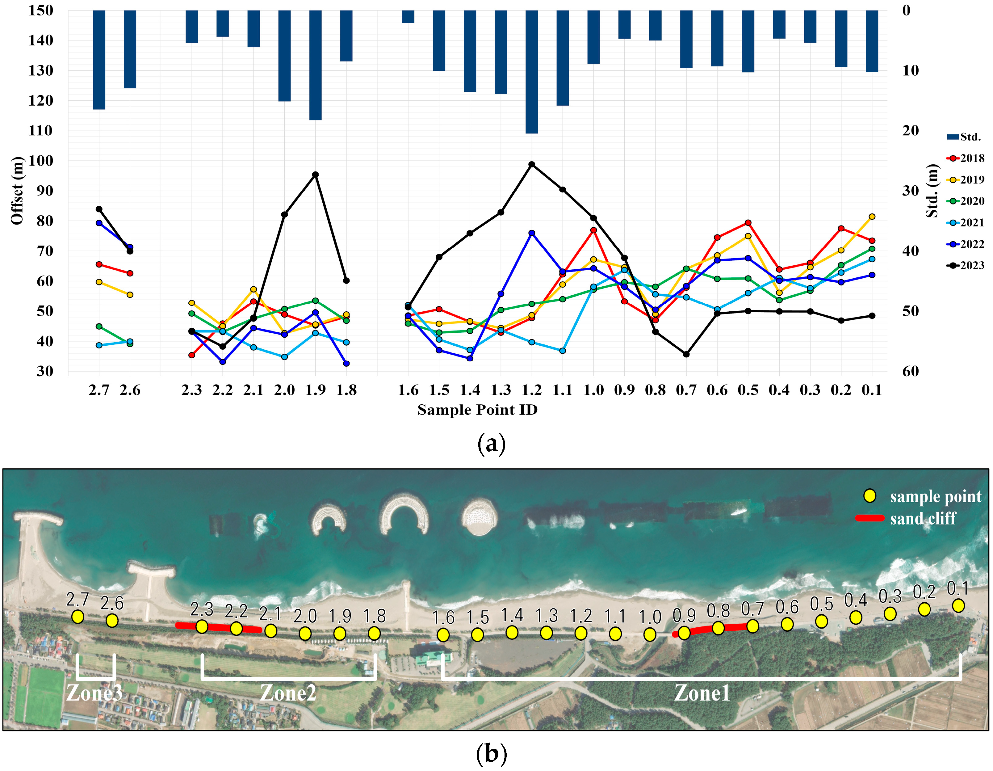
The point-specific offset analysis was followed to identify erosion-susceptible sections of the roadway. In Figure 12a, the ID of each sample point on the x–axis corresponds to its linear distance in kilometers from the starting point of the roadway. The left y–axis represents the annual mean offset, while the right y–axis indicates the standard deviation of all annual offsets. Also, in Figure 12b, the aerial photo illustrates the spatial locations of the sample points along the coastal roadway. This analysis shows that 14 out of 24 sample points experienced shoreline accretion between 2018 and 2023, resulting in a reduction of roadway vulnerability across approximately 58% of the coastal roadway. Specifically, the roadway sections from sample point ID 1.1 to ID 1.5, from ID 1.9 to ID 2.0, and at ID 2.7 exhibited notable increases in the mean offsets in 2022 and 2023, accompanied by higher standard deviations exceeding 10 m. These results imply not only increased sediment accumulation, but also spatial variability has occurred due to local topographic conditions or infrastructure interventions. In contrast, despite the erosion control structures, some roadway sections continued to experience shoreline erosion. For example, the roadway section from sample point ID 0.1 to ID 0.8 remained stable from 2018 to 2022, but a sharp decline in mean offset was observed in 2023. This implies that the erosion control structures may have limited spatial effectiveness.

For a more detailed assessment at the local scale, sub-analysis zones with greater shoreline variability were selectively defined, and vector offsets were measured at 10-m intervals. In Zone 1, three sub-analysis zones, which are Zone 1-A, Zone 1-B, and Zone 1-C, were defined for the annual offset analysis in

Table 7. Annual offset analysis in sub-analysis zones of Zone 1 (in meters).

	Zone 1-A		Zone 1-B		Zone 1-C
Year	Mean Offset	Std.	Mean Offset	Std.	Mean Offset	Std.
2018	58.3	1.0	56.0	8.6	49.8	1.9
2019	61.0	5.5	55.4	5.4	47.6	5.9
2020	65.0	5.1	52.7	3.0	42.8	1.1
2021	54.3	1.5	40.0	4.4	39.9	4.1
2022	58.4	3.8	68.0	4.8	38.2	4.6
2023	36.7	1.9	93.3	5.8	71.0	7.4

and for the point-specific offset analysis in Figure 13. The overall trends of shoreline changes indicate that Zones 1-B and 1-C have shoreline accretion, whereas, Zone 1-A has a continuous shoreline recession despite the presence of the erosion control structures. In Table 7, shoreline distances in Zone 1-A remained relatively stable from 2018 to 2022, with mean offsets exceeding 58.3 m in most years, except for 2021. However, in 2023, the mean offset sharply decreased due to the construction of detached and submerged breakwaters in 2022 and 2023. Intensified wave activity caused shoreline erosion between sample point IDs 0.71 and 0.93, resulting in the formation of sand cliffs and increased roadway vulnerability in Figure 13.

The coastal roadways in Zone 1-B and Zone 1-C, adjacent to the detached and submerged breakwaters, each span approximately 200 m (Figure 13b). In Table 7, Zone 1-B exhibited greater variation in both mean offsets and standard deviations compared to the other sub-analysis zones. Between 2018 and 2021, the mean offset decreased from 56.0 m to 40.0 m. However, following the construction of submerged breakwaters in 2022, rapid sediment deposition increased the mean offset to 93.3 m by 2023, indicating reduced roadway vulnerability. In Zone 1-C, the mean offset consistently decreased from 2018 to 2022. In Table 7, the mean offsets between 2021 and 2022 were below 40 m, indicating high roadway vulnerability. However, in 2023, shoreline accretion between sample points ID 1.35 and 1.50 resulted in a 32.8 m increase in the mean offset, reaching 71.0 m. Also, the standard deviation sharply rose to 7.4 m. Similar to Zone 1-B, this shoreline accretion is attributed to the submerged and detached breakwaters, leading to reduced roadway vulnerability.

The coastal roadway in Zone 2-A includes sand cliffs along the shoreline (Figure 14b). According to

Table 8. Annual offset analysis within sub-analysis zones of Zones 2 and 3 (in meters).

	Zone 2-A		Zone 3-A
Year	Mean Offset	Std.	Mean Offset	Std.
2018	48.0	6.8	68.5	3.2
2019	49.4	5.4	57.1	1.4
2020	47.4	3.2	39.9	2.3
2021	39.0	2.7	37.5	1.2
2022	39.7	4.9	73.8	2.6
2023	55.5	19.7	74.3	4.7

, the mean offset increased from 48.0 m in 2018 to 49.4 m in 2019, even though construction of the thermal power plant began in late 2018. However, after the breakwater was built in 2021, the mean offset sharply decreased to 39.0 m, indicating that the roadway became more vulnerable. In 2023, the mean offset rose to 55.5 m, which implies that shoreline accretion occurred due to the detached breakwaters constructed in 2022. Nevertheless, the high standard deviation of 19.7 m implies that shoreline accretion was spatially irregular along the roadway. The point-specific analysis in Figure 14 confirms that significant shoreline accretion was observed around sample point ID 2.0, resulting in a standard deviation exceeding 10 m. In contrast, for the remainder of the roadway, relatively limited shoreline accretion was observed with a standard deviation below 10 m. Also, the sand cliffs between ID 2.14 and 2.37 appear to have contributed to persistent vulnerability. In Zone 3-A, the roadway between the two breakwaters extends from sample points ID 2.60 to 2.70. As shown in Table 8, the mean offset dropped from 68.5 m in 2018 to 37.5 m in 2021, indicating significant shoreline erosion. However, in 2023, the mean offset increased to 74.3 m, reflecting a reduction in roadway vulnerability. Figure 14 also illustrates that geomorphological changes followed the construction of breakwaters between 2021 and 2023. Each sample point recorded a standard deviation exceeding 13 m. Concentrated wave energy between the breakwaters likely accelerated erosion from 2019 to 2021, but the completion of the structures and beach nourishment appears to have mitigated this effect, promoted shoreline recovery and improved road stability.

4. Discussion

In this study, the novel geospatial approach was developed to assess roadway vulnerability in relation to shoreline changes. Although numerous GIS-based approaches have been developed to support roadway reinforcement and planning susceptible to shoreline retreat, key limitation remains in the lack of a standardized referencing and data management framework for associating roadway asset information with shoreline change analysis results. Furthermore, conventional analysis methods for shoreline changes are often sensitive to the geometric complexity of shorelines and roadway centerlines in GIS. The proposed approach addresses these limitations by integrating the LRS-based geospatial framework with the VOA method within GIS, thereby enabling consistent and spatially explicit assessments of coastal roadway vulnerability.

In the case study, the proposed approach successfully identified both erosion-prone and recovered sections along the Maengbang coastal roadway. By associating the linear positions of the roadway with spatiotemporal shoreline change analysis, the proposed approach facilitates the visually identification of roadway vulnerability from 2018 to 2023. Specifically, the mean offset increased from 48.2 m in 2021 to 62.9 m in 2023, indicating shoreline recovery following the construction of breakwater. However, the increased standard deviation implies that the accretion is spatially uneven. These analysis results, which closely reflect to the actual erosion pattern of Maengbang Beach, indicate that the proposed approach can practically support for sustainable maintenance of coastal roadways. For example, the proposed approach facilitates the identification of erosion-prone roadway sections, thereby enabling data-driven decision for roadway maintenance and structural reinforcement. The spatiotemporal shoreline change analysis also allows for the detection of high-risk coastal areas along roadway, supporting the timely implementation of preventive measures. Furthermore, the proposed approach can assist local authorities in prioritizing the placement of protective structures such as breakwaters and beach nourishment interventions.

However, as the proposed approach is developed based on a geospatial framework within GIS, the analysis results are inherently influenced by positional uncertainties in both the roadway centerline map and shoreline datasets. In addition, temporal uncertainties arise from seasonal variations in meteorological and tidal conditions, potentially affecting the consistency of shoreline positions across different time periods. To mitigate uncertainty impacts on the analysis results, spatial dataset with highly reliable were used in this study. In South Korea, 1:5000 scale maps serve as base maps for roadway management and planning. In addition, the shoreline datasets were extracted from high-resolution of aerial orthophotos acquired under appropriate meteorological and tidal conditions. Therefore, the spatial data are considered sufficiently reliable to analyze the long-term shoreline change analysis. However, when applying the proposed approach to other coastal regions, careful consideration of local data accuracy, acquisition time, and environmental variability will be essential to ensure analytical robustness and comparability.

5. Conclusions

This paper presented the novel geospatial approach to analyze coastal roadway vulnerability to shoreline changes. Compared with existing approaches, the main novelty lies in its ability to integrate roadway asset information and shoreline change analysis results. The LRS, implemented within GIS, provides a comprehensive framework for integrating roadway and shoreline data into the linear domain of a roadway spatial database. Specifically, the linear referencing method defines the linear locations of roadway sections and their adjacent assets along a roadway network, as well as designates sample points along the roadway centerline at a predefined interval for shoreline change analysis. The VOA method is subsequently applied to quantitatively analyze historical changes in shoreline positions relative to the coastal roadway. In the analysis, the mean and standard deviation of vector offsets represent the magnitude of positional shift and its variability, respectively. Based on these metrics, roadway sections and adjacent assets at high-risk of shoreline recession can be identified and assessed for effective coastal roadway management.

The proposed approach was applied to a coastal roadway significantly affected by shoreline changes, mainly driven by climate change and anthropic activities such as the construction of thermal plants, berthing facilities, and erosion control structures. The case study demonstrates that the proposed approach enables the spatial data-driven assessment of roadway vulnerability by identifying both erosion-susceptible and shoreline recovered roadway sections. However, even though reliable spatial datasets were used in the proposed approach, the accuracy of the analysis results is inherently affected by positional and temporal uncertainties in the spatial data quality of roadway centerline maps and shoreline datasets. Therefore, to deal with problems concerning the qualities of spatial data as well as of analysis results, future research should expand to develop a methodology to formulate characterization and propagation of positional uncertainties in operational GIS-based applications. Such advancements would support more informed decision-making for long-term coastal roadway maintenance and adaptive infrastructure planning.

References

1. Cosby, A.; Lebakula, V.; Smith, C.; Wanik, D.; Bergene, K.; Rose, A.; Swanson, D.; Bloom, D. Accelerating growth of human coastal populations at the global and continent levels: 2000–2018. Sci. Rep. 2024, 14, 22489. [Google Scholar] [CrossRef] [PubMed]
2. Creel, L. Ripple Effects: Population and Coastal Regions; Population Reference Bureau: Washington, DC, USA, 2003. [Google Scholar]
3. Martínez, M.L.; Intralawan, A.; Vázquez, G.; Pérez-Maqueo, O.; Sutton, P.; Landgrave, R. The coasts of our world: Ecological, economic and social importance. Ecol. Econ. 2007, 63, 254–272. [Google Scholar] [CrossRef]
4. Newton, A.; Icely, J.; Cristina, S.; Perillo, G.M.; Turner, R.E.; Ashan, D.; Cragg, S.; Luo, Y.; Tu, C.; Li, Y. Anthropogenic, direct pressures on coastal wetlands. Front. Ecol. Evol. 2020, 8, 144. [Google Scholar] [CrossRef]
5. Mentaschi, L.; Vousdoukas, M.I.; Pekel, J.-F.; Voukouvalas, E.; Feyen, L. Global long-term observations of coastal erosion and accretion. Sci. Rep. 2018, 8, 12876. [Google Scholar] [CrossRef]
6. Anthony, E.J.; Marriner, N.; Morhange, C. Human influence and the changing geomorphology of Mediterranean deltas and coasts over the last 6000 years: From progradation to destruction phase? Earth-Sci. Rev. 2014, 139, 336–361. [Google Scholar] [CrossRef]
7. Brandes, H.; Doygun, O.; Francis, O.; Zhang, G.; Rossi, C.; Yang, L.; Togia, H. CRESI: A susceptibility index methodology to assess roads threatened by coastal erosion. Ocean. Coast. Manag. 2021, 213, 105845. [Google Scholar] [CrossRef]
8. Behr, A.; Berglund, E.; Sciaudone, E. Effectiveness of indicators for assessing the vulnerability of barrier island highways. Transp. Res. Part D Transp. Environ. 2022, 105, 103234. [Google Scholar] [CrossRef]
9. Douglass, S.L.; Webb, B.M. Highways in the Coastal Environment: Hydraulic Engineering Circular Number 25; Federal Highway Administration. Office of Bridges and Structures: Washington, DC, USA, 2020. [Google Scholar]
10. Darestani, Y.M.; Webb, B.; Padgett, J.E.; Pennison, G.; Fereshtehnejad, E. Fragility analysis of coastal roadways and performance assessment of coastal transportation systems subjected to storm hazards. J. Perform. Constr. Facil. 2021, 35, 04021088. [Google Scholar] [CrossRef]
11. Velasquez-Montoya, L.; Sciaudone, E.J.; Smyre, E.; Overton, M.F. Vulnerability indicators for coastal roadways based on barrier island morphology and shoreline change predictions. Nat. Hazards Rev. 2021, 22, 04021003. [Google Scholar] [CrossRef]
12. Azevedo de Almeida, B.; Mostafavi, A. Resilience of infrastructure systems to sea-level rise in coastal areas: Impacts, adaptation measures, and implementation challenges. Sustainability 2016, 8, 1115. [Google Scholar] [CrossRef]
13. Peponi, A.; Morgado, P.; Trindade, J. Combining artificial neural networks and GIS fundamentals for coastal erosion prediction modeling. Sustainability 2019, 11, 975. [Google Scholar] [CrossRef]
14. Fannassi, Y.; Ennouali, Z.; Hakkou, M.; Benmohammadi, A.; Al-Mutiry, M.; Elbisy, M.S.; Masria, A. Prediction of coastal vulnerability with machine learning techniques, Mediterranean coast of Tangier-Tetouan, Morocco. Estuar. Coast. Shelf Sci. 2023, 291, 108422. [Google Scholar] [CrossRef]
15. Fogarin, S.; Zanetti, M.; Dal Barco, M.K.; Zennaro, F.; Furlan, E.; Torresan, S.; Pham, H.V.; Critto, A. Combining remote sensing analysis with machine learning to evaluate short-term coastal evolution trend in the shoreline of Venice. Sci. Total Environ. 2023, 859, 160293. [Google Scholar] [CrossRef]
16. Tzepkenlis, A.; Grammalidis, N.; Kontopoulos, C.; Charalampopoulou, V.; Kitsiou, D.; Pataki, Z.; Patera, A.; Nitis, T. An integrated monitoring system for coastal and Riparian areas based on remote sensing and machine learning. J. Mar. Sci. Eng. 2022, 10, 1322. [Google Scholar] [CrossRef]
17. Drejza, S.; Bernatchez, P.; Marie, G.; Friesinger, S. Quantifying road vulnerability to coastal hazards: Development of a synthetic index. Ocean. Coast. Manag. 2019, 181, 104894. [Google Scholar] [CrossRef]
18. Fraser, C.; Bernatchez, P.; Dugas, S. Development of a GIS coastal land-use planning tool for coastal erosion adaptation based on the exposure of buildings and infrastructure to coastal erosion, Québec, Canada. Geomat. Nat. Hazards Risk 2017, 8, 1103–1125. [Google Scholar] [CrossRef]
19. Gao, S.; Zhai, W. Assessing adaptation planning strategies of interconnected infrastructure under sea-level rise by economic analysis. Front. Archit. Res. 2023, 12, 892–905. [Google Scholar] [CrossRef]
20. Aouiche, I.; Daoudi, L.; Anthony, E.J.; Sedrati, M.; Ziane, E.; Harti, A.; Dussouillez, P. Anthropogenic effects on shoreface and shoreline changes: Input from a multi-method analysis, Agadir Bay, Morocco. Geomorphology 2016, 254, 16–31. [Google Scholar] [CrossRef]
21. Özpolat, E.; Demir, T. The spatiotemporal shoreline dynamics of a delta under natural and anthropogenic conditions from 1950 to 2018: A dramatic case from the Eastern Mediterranean. Ocean. Coast. Manag. 2019, 180, 104910. [Google Scholar] [CrossRef]
22. Donadio, C.; Vigliotti, M.; Valente, R.; Stanislao, C.; Ivaldi, R.; Ruberti, D. Anthropic vs. natural shoreline changes along the northern Campania coast, Italy. J. Coast. Conserv. 2018, 22, 939–955. [Google Scholar] [CrossRef]
23. Del Río, L.; Gracia, F.J.; Benavente, J. Shoreline change patterns in sandy coasts. A case study in SW Spain. Geomorphology 2013, 196, 252–266. [Google Scholar] [CrossRef]
24. Morton, R. Coastal geoindicators of environmental change in the humid tropics. Environ. Geol. 2002, 42, 711–724. [Google Scholar]
25. Armah, F.A. GIS-based assessment of short term Shoreline changes in the coastal erosion-sensitive zone of Accra, Ghana. Res. J. Environ. Sci. 2011, 5, 643–654. [Google Scholar] [CrossRef]
26. Parthasarathy, K.; Deka, P.C. Remote sensing and GIS application in assessment of coastal vulnerability and shoreline changes: A review. ISH J. Hydraul. Eng. 2021, 27, 588–600. [Google Scholar] [CrossRef]
27. Cenci, L.; Disperati, L.; Persichillo, M.G.; Oliveira, E.R.; Alves, F.L.; Phillips, M. Integrating remote sensing and GIS techniques for monitoring and modeling shoreline evolution to support coastal risk management. GIScience Remote Sens. 2018, 55, 355–375. [Google Scholar] [CrossRef]
28. Albuquerque, M.; Espinoza, J.; Teixeira, P.; de Oliveira, A.; Corrêa, I.; Calliari, L. Erosion or coastal variability: An evaluation of the DSAS and the change polygon methods for the determination of erosive processes on sandy beaches. J. Coast. Res. 2013, 1710–1714. [Google Scholar] [CrossRef]
29. Rogers, S.S.; Sandweiss, D.H.; Maasch, K.A.; Belknap, D.F.; Agouris, P. Coastal change and beach ridges along the northwest coast of Peru: Image and GIS analysis of the Chira, Piura, and Colan beach-ridge plains. J. Coast. Res. 2004, 20, 1102–1125. [Google Scholar] [CrossRef]
30. Heo, J.; Kim, J.H.; Kim, J.W. A new methodology for measuring coastline recession using buffering and non-linear least squares estimation. Int. J. Geogr. Inf. Sci. 2009, 23, 1165–1177. [Google Scholar] [CrossRef]
31. Li, R.; Liu, J.-K.; Felus, Y. Spatial modeling and analysis for shoreline change detection and coastal erosion monitoring. Mar. Geod. 2001, 24, 1–12. [Google Scholar] [CrossRef]
32. Anfuso, G.; Bowman, D.; Danese, C.; Pranzini, E. Transect based analysis versus area based analysis to quantify shoreline displacement: Spatial resolution issues. Environ. Monit. Assess. 2016, 188, 1–14. [Google Scholar] [CrossRef]
33. Smith, M.J.; Cromley, R.G. Measuring historical coastal change using GIS and the change polygon approach. Trans. GIS 2012, 16, 3–15. [Google Scholar] [CrossRef]
34. Manno, G.; Re, C.L.; Basile, M.; Ciraolo, G. A new shoreline change assessment approach for erosion management strategies. Ocean. Coast. Manag. 2022, 225, 106226. [Google Scholar] [CrossRef]
35. ISO 19148; Geographic Information—Linear Referencing. ISO: Geneva, Switzerland, 2021.
36. Heo, J.; Jeong, S.; Han, S.; Kim, C.; Hong, S.; Sohn, H.-G. Discrete displacement analysis for geographic linear features and the application to glacier termini. Int. J. Geogr. Inf. Sci. 2013, 27, 1631–1650. [Google Scholar] [CrossRef]
37. Goodchild, M.F.; Hunter, G.J. A simple positional accuracy measure for linear features. Int. J. Geogr. Inf. Sci. 1997, 11, 299–306. [Google Scholar] [CrossRef]
38. Lee, Y.; Chang, S.; Kim, J.; Kim, I. Estimation of Beach Profile Response on Coastal Hydrodynamics Using LSTM-Based Encoder–Decoder Network. J. Mar. Sci. Eng. 2024, 12, 2212. [Google Scholar] [CrossRef]
39. Jung, T.S. Sea Level Change due to Nonlinear Tides in Coastal Region. J. Korean Soc. Coast. Ocean. Eng. 2017, 29, 228–238. [Google Scholar] [CrossRef]
40. Jeong, W.M.; Cho, H.; Oh, S.H.; Kim, S.I. Temporal and spatial variations in the wave energy potential of the east coastal seas of Korea. J. Korean Soc. Coast. Ocean. Eng. 2013, 25, 311–316. [Google Scholar] [CrossRef]
41. Jeong, W.-M.; Oh, S.-H.; Cho, H.-Y.; Baek, W.-D. Characteristics of Waves Continuously Observed over Six Years at Offshore Central East Coast of Korea. J. Korean Soc. Coast. Ocean. Eng. 2019, 31, 88–99. [Google Scholar] [CrossRef]
42. Eum, H.-S.; Jeong, W.-M.; Chang, Y.S.; Oh, S.-H.; Park, J.-J. Wave energy in korean seas from 12-year wave hindcasting. J. Mar. Sci. Eng. 2020, 8, 161. [Google Scholar] [CrossRef]
43. Kim, J.; Chang, P.-H.; Kang, H.-S. A Study on The Effects of Long-Term Tidal Constituents on Surge Forecasting Along The Coasts of Korean Peninsula. J. Korean Soc. Coast. Ocean. Eng. 2022, 34, 222–232. [Google Scholar] [CrossRef]
Figure 1. Shoreline change analysis methods. (a) TBA, (b) ABA.
Land 14 01158 g001
Figure 2. Uncertainty sources in shoreline change analysis. (a) TBA, (b) ABA.
Land 14 01158 g002
Figure 3. Probability density function of a point along a line segment.
Land 14 01158 g003
Figure 4. Dual representation of a line buffer and a set of vector offsets from a line segment.
Land 14 01158 g004
Figure 5. Example of vector offset analysis between a baseline and a target line: (a) negative mean offset, (b) zero mean offset, and (c) positive mean offset, all with the same standard deviation.
Land 14 01158 g005
Figure 6. Comparison of the VOA and TBA methods. (a) Test dataset; (b) positional offset analysis result from VOA method; (c) positional offset analysis result from TBA method.
Land 14 01158 g006
Figure 7. Comparison of the VOA and ABA methods. (a) Test dataset; (b,c) positional offset analysis results from VOA method; (d,e) positional offset analysis results from ABA method.
Land 14 01158 g007
Figure 8. Linear referencing system for roadway management.
Land 14 01158 g008
Figure 9. Linear referencing method with VOA method for shoreline change analysis.
Land 14 01158 g009
Figure 10. Shorelines along Maengbang coastal roadways in 2018 and 2023.
Land 14 01158 g010
Figure 11. Example of a referent in LRS. (a) Road intersection; (b) Reporting spot (Maengbang-2).
Land 14 01158 g011
Figure 12. Point-specific offset analysis along the coastal roadway. (a) Shoreline offsets and standard deviation for sample points; (b) spatial locations of the sample points.
Land 14 01158 g012
Figure 13. Point-specific offset analysis within the sub-analysis zones of Zone 1. (a) Shoreline offsets and standard deviation for sample points; (b) spatial locations of the sample points.
Land 14 01158 g013
Figure 14. Point-specific offset analysis within the sub-analysis zones of Zones 2 and 3. (a) Shoreline offsets and standard deviation for sample points; (b) spatial locations of the sample points.
Land 14 01158 g014