Impacts of Ecological Restoration Projects on Ecosystem Carbon Storage of Tongluo Mountain Mining Area, Chongqing, in Southwest China

Abstract

Surface mining activities cause severe disruption to ecosystems, resulting in the substantial destruction of surface vegetation, the loss of soil organic carbon stocks, and a decrease in the ecosystem’s ability to sequester carbon. The ecological restoration of mining areas has been found to significantly enhance the carbon storage capacity of ecosystems. This study evaluated ecological restoration strategies in Chongqing’s Tongluo Mountain mining area by integrating GF-6 satellite multispectral data (2 m panchromatic/8 m multispectral resolution) with ground surveys across 45 quadrats to develop a quadratic regression model based on vegetation indices and the field-measured biomass. The methodology quantified carbon storage variations among engineered restoration (ER), natural recovery (NR), and unmanaged sites (CWR) while identifying optimal vegetation configurations for karst ecosystems. The methodology combined the high-spatial-resolution satellite imagery for large-scale vegetation mapping with field-measured biomass calibration to enhance the quantitative accuracy, enabling an efficient carbon storage assessment across heterogeneous landscapes. This hybrid approach overcame the limitations of traditional plot-based methods by providing spatially explicit, cost-effective monitoring solutions for mining ecosystems. The results demonstrate that engineered restoration significantly enhances carbon sequestration, with the aboveground vegetation biomass reaching 5.07 ± 1.05 tC/ha, a value 21% higher than in natural recovery areas (4.18 ± 0.23 tC/ha) and 189% greater than at unmanaged sites (1.75 ± 1.03 tC/ha). In areas subjected to engineered restoration, both the vegetation and soil carbon storage showed an upward trend, with soil carbon sequestration being the primary form, contributing to 81% of the total carbon storage, and with engineered restoration areas exceeding natural recovery and unmanaged zones by 17.6% and 106%, respectively, in terms of their soil carbon density (40.41 ± 9.99 tC/ha). Significant variations in the carbon sequestration capacity were observed across vegetation types. Bamboo forests exhibited the highest carbon density (25.8 tC/ha), followed by tree forests (2.54 ± 0.53 tC/ha), while grasslands showed the lowest values (0.88 ± 0.52 tC/ha). For future restoration initiatives, it is advisable to select suitable vegetation types based on the local dominant species for a comprehensive approach.

1. Introduction

The mining industry leads to drastic changes in land use/cover, causing the significant destruction of surface vegetation, the loss of soil organic carbon storage, a decrease in the ecosystem’s carbon sequestration capacity, and even negative feedback [1,2,3]. A series of ecological restoration measures used in mining areas to restore the ecological functions of the land and rebuild the soil carbon sink are of great significance for the neutralization of carbon in the regional atmosphere and thus an important carbon fixation measure [4]. The reclamation of abandoned mine land which has been damaged or is being damaged is not only an effective way to protect and use land resources rationally and restore their productivity but also an important action to increase the vegetation and soil carbon sinks, eliminate adverse effects on the ecosystem, and maintain ecosystem stability. The increase in carbon sinks in mining areas achieved through afforestation activities has been widely recognized [5,6]. In China, the ecological restoration of mining areas has gained importance due to its alignment with the national “dual carbon” goals (peak emissions by 2030, carbon neutrality by 2060) [7,8]. Despite progress, significant gaps remain in understanding how restoration outcomes vary across distinct geographical and climatic regions.

Previous studies on mining area restoration have predominantly focused on northern China, where arid climates (annual rainfall of <400 mm) and sparse populations simplify restoration efforts [4,9]. In these regions, the low precipitation slows soil erosion and organic carbon decomposition, allowing for the gradual natural recovery of vegetation [10]. However, water scarcity limits biomass accumulation, necessitating engineered interventions such as irrigation systems [4]. In stark contrast, southwest China—particularly Chongqing’s Tongluo Mountain area—faces a unique set of challenges due to its humid subtropical climate (annual rainfall of >1200 mm), karst topography, and dense population [1,11]. Here, heavy rainfall accelerates soil erosion in disturbed mining areas, washing away nutrient-rich topsoil and destabilizing slopes [2,12]. Karst landscapes are characterized by thin soil layers and rapid water infiltration. Mining activities have significantly increased soil erosion rates [13] and elevated the risk of stony desertification [14]. These factors further complicate vegetation restoration efforts, as shallow soils struggle to retain moisture and nutrients [15]. Additionally, a high population density intensifies land use conflicts, with agricultural and urban demands competing against ecological restoration efforts [16]. These regional disparities necessitate tailored strategies, yet comparative studies between northern and southern mining areas remain limited. Ecological restoration outcomes are profoundly influenced by methodological choices. Natural recovery—relying on spontaneous vegetation regrowth—is cost-effective but slow, particularly in highly degraded ecosystems [5]. Engineered restoration, involving soil stabilization, organic amendments, and the strategic planting of native species, has shown promise in accelerating carbon sequestration [6]. For instance, in the Shiyang River Basin (northern China), engineered interventions increased the soil carbon stocks by 35% more within a decade compared to natural recovery [9]. However, the effectiveness of such approaches in high-rainfall regions remains understudied.

The vegetation type further dictates the carbon sequestration potential. Bamboo forests, with their rapid growth rates and extensive root systems, exhibit higher carbon fixation capacities than grasslands or shrublands [17,18]. In Guangxi Province, bamboo plantations sequester 6.8 tC/ha annually, nearly double that of mixed forests [17]. Such findings highlight the importance of species selection in restoration planning, yet no studies have systematically compared the vegetation-specific carbon dynamics in southwest China’s mining areas.

The most accurate method for measuring an ecosystem’s carbon storage is undoubtedly the traditional plot survey method, but this method is only applicable on a small scale and may cause changes to the ecological environment to a certain extent [19,20]; the model estimation method estimates the carbon storage of large-scale forest ecosystems using mathematical models and is limited by the assumptions and simplifications in the model’s mechanisms, and the error is relatively large [21,22,23]; and remote sensing technology has become an important tool for monitoring vegetation growth, land cover changes, and surface deformation. By analyzing remote sensing data, researchers can evaluate the effectiveness of ecological restoration projects [24,25,26]. Remote sensing data with different resolutions, such as data from MODIS, Landsat TM, Landsat ETM, Landsat OLI, SPOT, and Quick Bird, are widely used [8,24,25,27,28,29,30,31,32,33]. The Gaofen-6 satellite (GF-6) was successfully launched by China on 2 June 2018 and is mainly used in precision agriculture observation, forest resource surveys, and other industries. The satellite is equipped with a 2 m panchromatic/8 m multispectral high-resolution camera, enabling precise vegetation structure characterization. Recent studies have validated its reliability: Yan et al. (2022) [6] demonstrated strong correlations (R² = 0.67–0.82) between the GF-6-derived NDVI and ground-measured aboveground biomass in forestry applications, outperforming Landsat-8 in heterogeneous terrains [24]. Additionally, Zhang et al. (2020) [8] confirmed GF-6’s capability to detect subtle vegetation recovery signals in mining areas, with a 15–20% improvement in the classification accuracy compared to that of SPOT-6 [30]. Despite these advantages, GF-6 remains underutilized in high-rainfall regions like southwest China, where the cloud cover and rapid vegetation growth complicate data acquisition. To address this gap, this paper mainly used GF-6 satellite remote sensing data combined with ground plot surveys to quantify the difference in the resulting carbon storage between natural recovery and engineering restoration after the closure of the mining area in Shichuan Town, Tongluo Mountain, Chongqing, providing methods and a basis for estimating the carbon sequestration potential of mining area ecological restoration in this area.

2. Study Area, Data, and Methods

Figure 1 illustrates the overall workflow of the methodology employed in this study, from data acquisition and processing to biomass modeling and carbon stock estimation.

2.1. Study Area

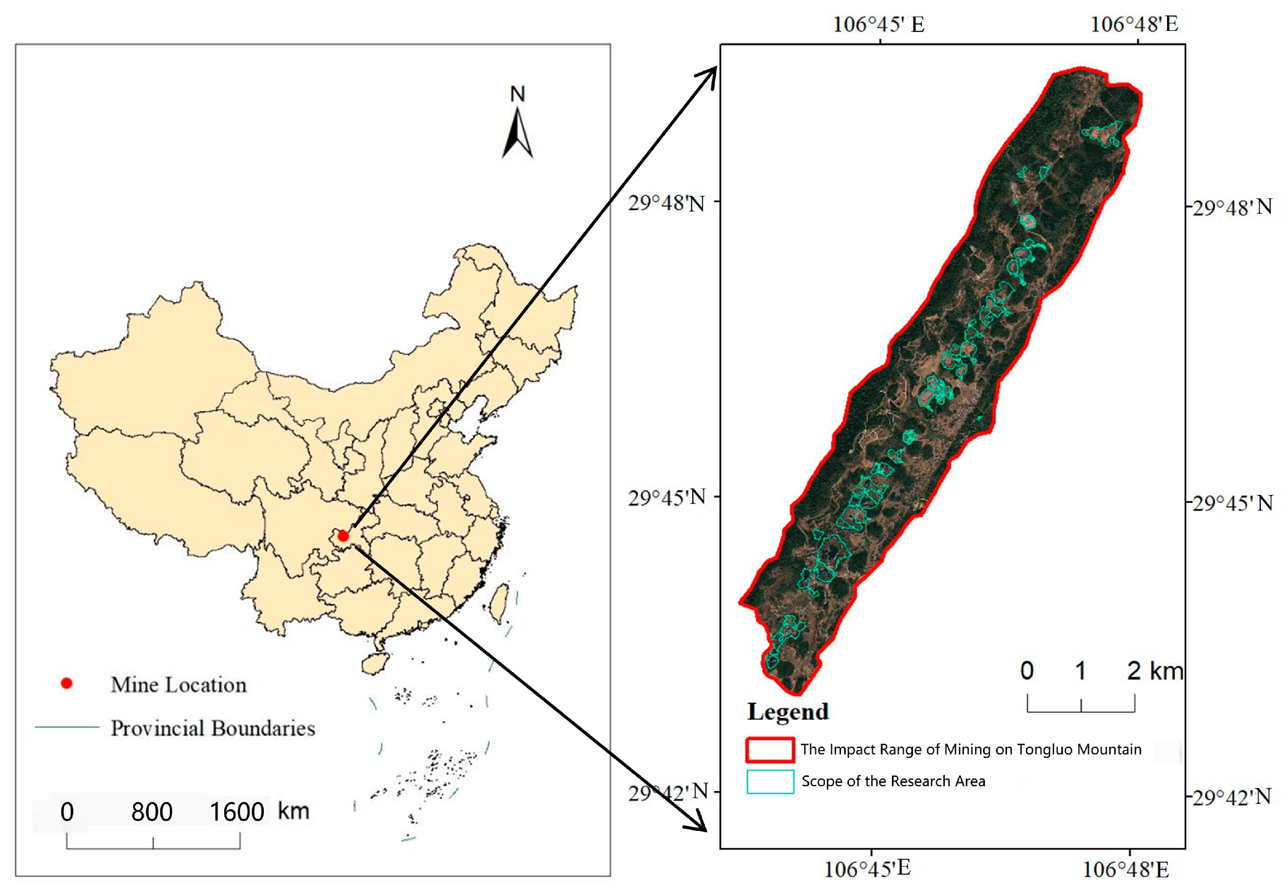
Tongluo Mountain is one of the “Four Mountains” in the main urban area of Chongqing and is one of two mountain ranges in the Eastern Sichuan parallel fold mountain and valley region. It is 260 km long and 5 to 10 km wide, with an average altitude of 600 to 1000 m, and the highest peak, Wanfeng Mountain, is 1054 m above sea level. The abandoned open-pit mine area of Tongluo Mountain is located in Shichuan Town and Yufengshan Town, Yubei District, Chongqing, with geographical coordinates ranging from an east longitude of 106°43′20″ to 106°48′14″ and a north latitude of 29°43′10″ to 29°49′12″, covering a total area of 24.15 square kilometers. There are 55 mines concentrated in this area, with the total area of the damaged mined land being 222.11 hectares. There are three mines larger than 10 hectares (the largest one is 25.83 hectares). All the other mines are less than 10 hectares, with 15 mines being less than 1 hectare, and the average mine area is 4.04 hectares (Figure 2). Located in Yubei District, the urban core of Chongqing, the study area epitomizes the conflict between rapid urbanization and ecological conservation. Situated merely 15 km from the Jiangbei CBD of Liangjiang New Area, the mine complex is surrounded by 12 villages and 3 towns within a 3 km radius. This creates a unique spatial matrix where derelict mining lands, prime farmland, and emerging residential zones are intricately interwoven. Such peri-urban characteristics make the site not only representative of mining-induced ecological degradation but also a microcosm of human–nature interactions under intense urbanization pressures. Research on ecological restoration in this human-dominated landscape will provide critical insights for managing “mine-urban” ecosystems.

It is important to note that within the Tongluo Mountain mining area, the sites selected for engineered ecological restoration projects are typically those presenting significant safety hazards and exhibiting severe initial degradation, such as unstable slopes, severe erosion, and minimal to no natural vegetation cover. These conditions represent an inherently less favorable starting point for ecosystem recovery compared to areas left for natural recovery or remaining unmanaged. Engineered restoration involves comprehensive interventions, including terrain reshaping, soil protection and repair, deliberate vegetation restoration, the development of accompanying infrastructure, and ongoing management. In contrast, areas designated for natural recovery have typically experienced less intensive initial disturbances and receive minimal intervention beyond fencing to prevent access, relying primarily on passive ecological processes for recovery. The comparison between these restoration strategies in this study therefore reflects the outcomes of overcoming severe initial degradation through active intervention versus allowing for recovery through natural processes under potentially less challenging conditions.

2.2. Satellite Data

This paper employed GF-6 satellite imagery data for the study. The Gaofen-6 satellite (GF-6), launched successfully on 2 June 2018, is mainly utilized in areas such as precision agriculture observation and forestry resource surveys. The GF-6 satellite is equipped with a 2 m panchromatic/8 m multispectral high-resolution camera and a 16 m multispectral medium-resolution wide-swath camera. This research selected the 2 m panchromatic/8 m multispectral high-resolution data for analysis, undertaking a remote sensing estimation of the aboveground biomass in the study area. After panchromatic and multispectral fusion, the spatial resolution was enhanced to 2 m. The imagery covered the Tongluo Mountain area (Shichuan Town section) in Yubei District and was captured on 22 September 2021 (refer to Figure 2 for the remote sensing image), which was during the typical transition period from late summer to early autumn in this region, a time when vegetation is still in a robust growth phase.

The brightness values (DN) of the remote sensing imagery used to record the gray levels of ground objects needed to be radiometrically calibrated in the preprocessing stage to convert them into the absolute reflectance. During the preprocessing of the GF-6 satellite data, the DN values first needed to be transformed using radiometric calibration. Every type of remote sensing satellite, domestically and internationally, has corresponding gain and offset values based on the parameters of their sensors. Radiometric calibration is specifically performed by computing the gain and offset. The radiometric calibration formula for GF-6 was as shown in

Table 1. Radiometric calibration parameters for 2021 GF-6 satellite multispectral high-resolution camera.

Satellite Camera	B1		B2		B3		B4
	Gain	Bias	Gain	Bias	Gain	Bias	Gain	Bias
GF6 PMS	0.0821	0	0.0671	0	0.0518	0	0.031	0

Note: The data were sourced from the official website of the China Center for Resource Satellite Data and Application.

.

After applying the aforementioned formula and the parameters from the table, radiometric calibration was conducted for the GF-6 imagery covering the study area. Following radiometric calibration, the FLAASH model was employed to perform an atmospheric correction on the data, thereby mitigating the errors in the band reflectance obtained post-correction to derive the surface reflectance. Subsequently, DEM data were utilized for orthorectification. The precision of the rectification was validated using high-quality imagery from the Resource-3 satellite, with the error range calculated to be within one pixel, confirming that the rectification precision was high and satisfied the usage standards.

2.3. Ground Survey Data

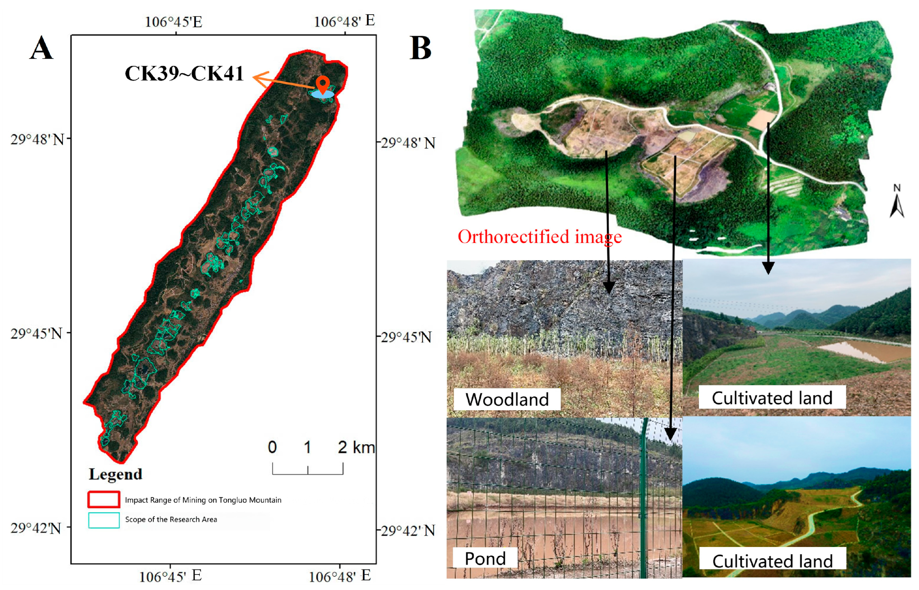
In early to mid-August 2021, a 10-day ground survey was conducted in the Tongluo Mountain area (Shichuan Town section) of Yubei District, covering a total of 15 plots, with GPS used for precise positioning at the center of each plot. This included 3 agricultural crop plots and 12 mountain vegetation plots, with the vegetation quadrats surveyed centered around each plot. Specifically, there were 16 tree quadrats dominated by Broussonetia papyrifera (paper mulberry) and Ficus virens (fig tree) (20 m × 20 m), 10 shrub quadrats dominated by Pyracantha fortuneana (firethorn) and Loropetalum chinense (Chinese witch hazel) (10 m × 10 m), and 10 herbaceous quadrats dominated by Artemisia (wormwood) and Solanum nigrum (black nightshade) (2 m × 2 m), as well as 9 agricultural crop quadrats representing Glycine max (soybean) and Zea mays (corn) (10 m × 10 m), totaling 45 vegetation quadrats. Of these, 75% of the samples (33 quadrats) were randomly selected for model establishment, and 25% (12 quadrats) were used for validation (Figure 3). The vegetation survey included detailed measurements and records of the height, north–south crown width, and base diameter of each standard plant and growth parameters such as the species frequency and plot coverage. The on-site sampling of the aboveground parts of standard plants of various vegetation types was conducted, and the aboveground biomass within the entire quadrat was calculated based on the dry and fresh weight of the survey samples. During the field survey, precise positioning was performed for each sampling point to obtain the latitude and longitude information of the sampling points.

2.4. Data Integration and Calculation of Carbon Storage

The methodological integration and synergistic use of the field survey data and remote sensing imagery were achieved through precise georeferencing. During the field survey phase (detailed in Section 2.3), the central coordinates of each sample plot were accurately determined using GPS technology. These geographic coordinates were meticulously recorded alongside the corresponding field-measured aboveground biomass value for that specific plot. Subsequently, these precise geographic coordinates served as the crucial spatial linkage mechanism between the ground truth data and the satellite observations. Utilizing the capabilities of ENVI software, the values of the selected predictor variables (in this case, the two chosen vegetation indices, though spectral band reflectance values could potentially be included as well) were extracted from the preprocessed and georectified GF-6 satellite imagery. This extraction was performed specifically at the pixel locations that spatially corresponded to the recorded center coordinates of each field plot. This co-location process effectively paired each ground-measured biomass value (dependent variable) with its corresponding set of remote sensing metrics (independent variables derived from satellite imagery), thereby creating the foundational dataset necessary for calibrating and subsequently validating the biomass estimation models.

To derive quantitative information from the satellite imagery for biomass estimation, the computation of vegetation indices was a primary step. In this study, the Band Math tool in ENVI 5.3 software was utilized to perform band operations on the preprocessed images to calculate eight types of vegetation indices. These included the NDVI (Normal Differential Vegetation Index), DVI (Differential Vegetation Index), GNDVI (Green Normal Differential Vegetation Index), RVI (Ratio Vegetation Index), SAVI (Soil-Adjusted Vegetation Index), MSAVI (Modified Soil-Adjusted Vegetation Index), EVI (Enhanced Vegetation Index), and ARVI (Atmospherically Resistant Vegetation Index) [34]. The formulas for calculating each vegetation index are presented in

Table 2. Vegetation index calculation formulas.

Vegetation Index	Formula
NDVI	$\mathrm{N}\mathrm{D}\mathrm{V}\mathrm{I}={\displaystyle \frac{{\mathrm{B}}_{\mathrm{N}\mathrm{I}\mathrm{R}}-{\mathrm{B}}_{\mathrm{R}\mathrm{E}\mathrm{D}}}{{\mathrm{B}}_{\mathrm{N}\mathrm{I}\mathrm{R}}-{\mathrm{B}}_{\mathrm{R}\mathrm{E}\mathrm{D}}}}$
DVI	$\mathrm{D}\mathrm{V}\mathrm{I}={\mathrm{B}}_{\mathrm{N}\mathrm{I}\mathrm{R}}-{\mathrm{B}}_{\mathrm{R}\mathrm{E}\mathrm{D}}$
RVI	$\mathrm{R}\mathrm{V}\mathrm{I}={\displaystyle \raisebox{1ex}{${\mathrm{B}}_{\mathrm{N}\mathrm{I}\mathrm{R}}$}\!\left/ \!\raisebox{-1ex}{${\mathrm{B}}_{\mathrm{R}\mathrm{E}\mathrm{D}}$}\right.}$
SAVI	$\mathrm{S}\mathrm{A}\mathrm{V}\mathrm{I}={\displaystyle \frac{({\mathrm{B}}_{\mathrm{N}\mathrm{I}\mathrm{R}}-{\mathrm{B}}_{\mathrm{R}\mathrm{E}\mathrm{D}})(1+\mathrm{L})}{{\mathrm{B}}_{\mathrm{N}\mathrm{I}\mathrm{R}}+{\mathrm{B}}_{\mathrm{R}\mathrm{E}\mathrm{D}}+\mathrm{L}}}$
MSAVI	$\mathrm{M}\mathrm{S}\mathrm{A}\mathrm{V}\mathrm{I}={\mathrm{B}}_{\mathrm{N}\mathrm{I}\mathrm{R}}+{\displaystyle \frac{1-\sqrt{{(2{\mathrm{B}}_{\mathrm{N}\mathrm{I}\mathrm{R}}+1)}^2-8({\mathrm{B}}_{\mathrm{N}\mathrm{I}\mathrm{R}}-{\mathrm{B}}_{\mathrm{R}\mathrm{E}\mathrm{D}})}}{2}}$
EVI	$\mathrm{E}\mathrm{V}\mathrm{I}=\left[({\mathrm{B}}_{\mathrm{N}\mathrm{I}\mathrm{R}}-{\mathrm{B}}_{\mathrm{R}\mathrm{E}\mathrm{D}})/({\mathrm{B}}_{\mathrm{N}\mathrm{I}\mathrm{R}}+6{\mathrm{B}}_{\mathrm{R}\mathrm{E}\mathrm{D}}-7.5{\mathrm{B}}_{\mathrm{B}\mathrm{L}\mathrm{U}\mathrm{E}}+1)\right]\times 2.5$
ARVI	$\mathrm{A}\mathrm{R}\mathrm{V}\mathrm{I}={\displaystyle \frac{{\mathrm{B}}_{\mathrm{N}\mathrm{I}\mathrm{R}}-(2{\mathrm{B}}_{\mathrm{R}\mathrm{E}\mathrm{D}}-{\mathrm{B}}_{\mathrm{B}\mathrm{L}\mathrm{U}\mathrm{E}})}{{\mathrm{B}}_{\mathrm{N}\mathrm{I}\mathrm{R}}+(2{\mathrm{B}}_{\mathrm{R}\mathrm{E}\mathrm{D}}-{\mathrm{B}}_{\mathrm{B}\mathrm{L}\mathrm{U}\mathrm{E}})}}$

${\mathrm{B}}_{\mathrm{N}\mathrm{I}\mathrm{R}}$ represents the near-infrared band; ${\mathrm{B}}_{\mathrm{R}\mathrm{E}\mathrm{D}}$ the red band; and ${\mathrm{B}}_{\mathrm{B}\mathrm{L}\mathrm{U}\mathrm{E}}$ the blue band.

. Additionally, 36 band combination factors were extracted from the image data, as detailed in

Table 3. Functional expressions of conventional statistical models.

Number	Model Type	Expression
1	Linear Function	$\mathrm{y}={\mathrm{b}}_0+{\mathrm{b}}_1\mathrm{x}$
2	Power Function	$\mathrm{y}={\mathrm{b}}_0{\mathrm{x}}^{{\mathrm{b}}_1}$
3	Inverse Function	$\mathrm{y}={\mathrm{b}}_0+{\displaystyle \frac{{\mathrm{b}}_1}{\mathrm{x}}}$
4	Logarithmic Function	$\mathrm{y}={\mathrm{b}}_0+{\mathrm{b}}_1\ln \mathrm{x}$
5	Exponential Function	$\mathrm{y}={\mathrm{b}}_0{\mathrm{e}}^{{\mathrm{b}}_1\mathrm{x}}$
6	S-Shaped Curve Function	$\mathrm{y}={\mathrm{e}}^{({\mathrm{b}}_0+{\displaystyle \raisebox{1ex}{${\mathrm{b}}_1$}\!\left/ \!\raisebox{-1ex}{$\mathrm{x}$}\right.})}$
7	Quadratic Function	$\mathrm{y}={\mathrm{b}}_0+{\mathrm{b}}_1\mathrm{x}+{\mathrm{b}}_2{\mathrm{x}}^2$
8	Cubic Function	$\mathrm{y}={\mathrm{b}}_0+{\mathrm{b}}_1\mathrm{x}+{\mathrm{b}}_2{\mathrm{x}}^2+{\mathrm{b}}_3{\mathrm{x}}^3$

Note: $b_1$, $b_2$, $b_3$, and $b_4$ are the model parameters, $y$ is the dependent variable (estimated aboveground biomass), and $x$ is the independent variable (remote sensing modeling factor).

. This study calculated the Pearson correlation coefficients between the measured plot biomass values and the 44 variables, which included the 8 vegetation indices and 36 band factors. Factors with insignificant correlations were preliminarily screened out. Ultimately, this study selected the 2 vegetation index variables exhibiting the strongest correlations as the modeling factors for the biomass estimation model.

Using the foundational dataset created by pairing biomass measurements with the selected remote sensing factors, relevant statistical analyses were conducted in SPSS (version 27.0) software. These included establishing univariate curve regression models (SCRM), using the selected vegetation indices individually, as well as multivariate linear regression models (MLRM) employing combinations of the four spectral band reflectances and the selected vegetation indices. The best fitting model was selected based on the determination coefficient (R²) and the root mean square error (RMSE). Eight conventional statistical models, a multiple stepwise regression (MSR), and a partial least squares regression (PLSR) were chosen to construct the aboveground biomass estimation model for the study area. A PLSR model integrates the advantages of multiple linear regression, principal component analysis, and canonical correlation analysis, which can avoid potential issues such as a non-normal distribution of the data, uncertainty in the factor structure, and model non-identifiability.

The performance and predictive accuracy of the developed biomass estimation models were primarily assessed using the determination coefficient (R²), root mean square error (RMSE), and mean absolute error (MAE), calculated against the independent validation dataset. These metrics were used to verify and evaluate the model’s precision and to select the best fitting model. The closer the R² value was to 1, the better the model explained the variance in the observed biomass and the better the model fit the data. The smaller the RMSE and MAE values, the higher the estimation accuracy. The calculation formulas were as follows:

$$R^2=1-{\displaystyle \frac{{\displaystyle \sum _{i=1}^n{(y_i-{\widehat{y}}_i)}^2}}{{\displaystyle \sum _{i=1}^n{(y_i-\widehat{y})}^2}}}$$

(1)

$$RMSE=\sqrt{{\displaystyle \frac{1}{n}}{\displaystyle \sum _{i=1}^n{(y_i-{\widehat{y}}_i)}^2}}$$

(2)

$$MAE={\displaystyle \frac{1}{n}}{\displaystyle \sum _{i=1}^n\left|y_i-{\widehat{y}}_i\right|}$$

(3)

where $y_i$ is the predicted value for the ith validation sample, ${\widehat{y}}_i$ is the measured value for the ith validation sample, and n = 10 is the number of validation samples.

3. Results and Analysis

3.1. Construction of Aboveground Vegetation Biomass Estimation Model

The vegetation index was positively correlated with the aboveground biomass measured on the ground in the study area. A remote sensing estimation model for the aboveground mountain vegetation biomass was established using the SCRM method; see

Table 4. Results for regression models.

Regression Model	Significance	R2	RMSE (tC/ha)	MAE (tC/ha)
$\mathrm{y}=2123.870(GNDVI{)}^2-2245.564\left(GNDVI\right)+623.666$	0.002	0.521	1.176	1.089
$\mathrm{y}=389.765\left(GNDVI\right)-170.973$	0.002	0.376	3.589	2.887
$\mathrm{y}=15.623e^{0.168\left(RvI\right)}$	0.002	0.396	2.675	2.382
$\mathrm{y}=8.982\left(\mathrm{R}\mathrm{V}\mathrm{I}\right)-2.128$	0.003	0.356	3.896	3.569

. Below are several models with good fitting effects and their accuracies, all of which passed the significance level test. After the comprehensive analysis of the R² and RMSE of each model, for mountain vegetation, we found that the quadratic equation model based on the GNDVI had the best correlation, with a determination coefficient, R², of 0.521. The model was validated for accuracy using a reserved sample that was not used in the modeling and had a root mean square error of 1.176 tC/ha and a mean absolute error of 1.089 tC/ha.

Based on the reflectance of four bands and the vegetation indices, the multiple stepwise regression method was used to select independent variables to establish the following regression model. The model’s accuracy was not as good as that of the SCRM. Therefore, the quadratic model based on the GNDVI was chosen for the inversion of the aboveground biomass of mountain vegetation, and the results show that the aboveground biomass of the vegetation in the study area was 3.68 tC/ha.

$$\mathrm{y}=2123.870(GNDVI{)}^2-2245.564\left(GNDVI\right)+623.666$$

(4)

3.2. The Spatial Distribution of the Aboveground Vegetation Biomass

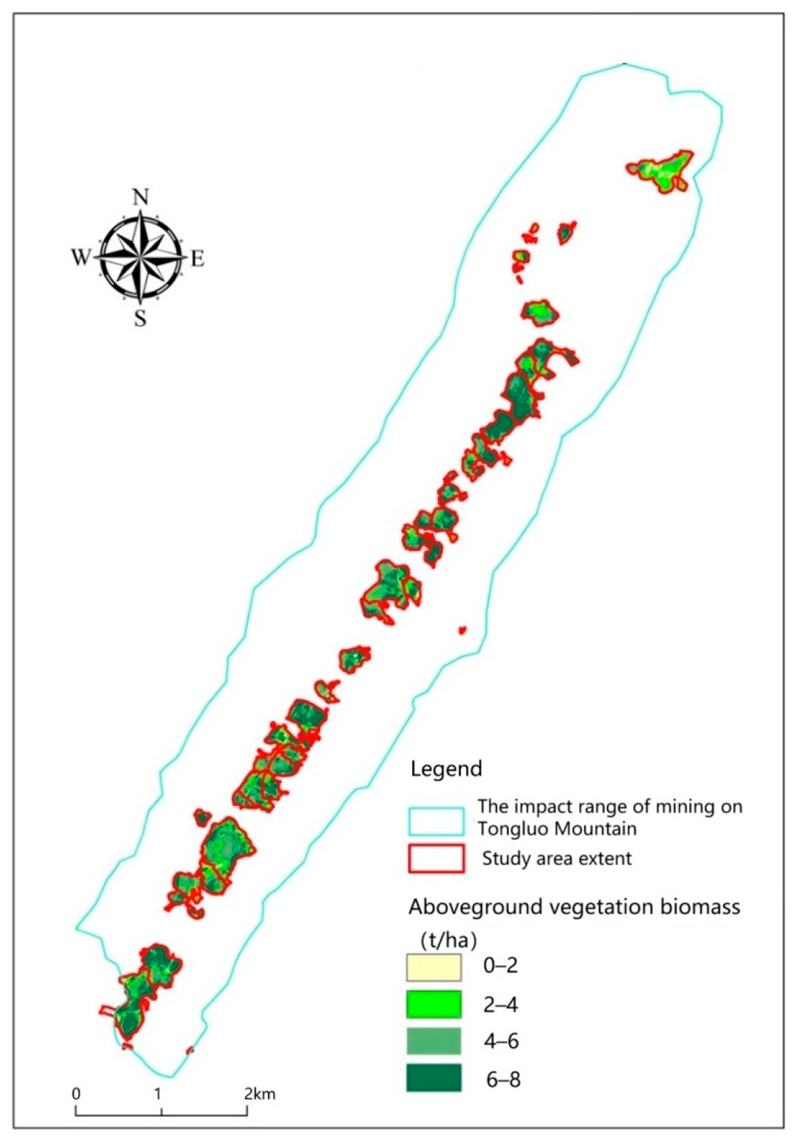
Incorporating the calculation results for the study area, ENVI 5.3 software was used to perform the remote sensing inversion of the aboveground biomass (AGB) of mountain vegetation in the study area. The estimated results for the aboveground biomass were divided into four grades according to the range of values, and a spatial distribution map of the aboveground vegetation biomass in the study area was produced, and the results were statistically analyzed using ArcGIS 10.2 software (Figure 4).

The biomass of forest communities is the most direct manifestation of the quality and functionality of the forest ecosystem structure, and it is a comprehensive reflection of the environmental quality of forest ecosystems. The quantitative estimation of a forest’s biomass provides an important reference for global carbon storage and carbon cycle research. The biomass data for each mine were exported for analysis, as shown in

Table 5. Aboveground biomass of vegetation in mining areas.

Number	Mining Type	Year of Closure	Year of Completion of Restoration	Restoration Strategy	Area (ha)	Aboveground Biomass (tC)	Average Biomass (tC/ha)
1	Quarry	2013	2021	ER	4.68	20.40	4.36
2	Limestone	2012	/	CWR	3.18	5.66	1.78
3	Quarry	2010	2018	NR	5.33	22.01	4.13
4	Limestone	2010	/	CWR	2.16	3.28	1.52
5	Limestone	2008	/	CWR	0.08	0.09	1.13
6	Limestone	2012	/	CWR	0.16	0.29	1.78
7	Quarry	2010	2022	ER	8.85	31.59	3.57
8	Quarry	2013	2021	ER	3.71	17.36	4.68
9	Quarry	2012	2021	ER	1.62	9.22	5.69
10	Quarry	2013	2021	ER	4.96	25.40	5.12
11	Quarry	2013	2021	ER	0.17	0.63	3.68
12	Limestone	2011	/	CWR	1.85	1.65	0.89
13	Limestone	2012	/	CWR	0.49	0.62	1.25
14	Quarry	2013	2021	ER	9.51	41.46	4.36
15	Limestone	2011	/	CWR	6.97	24.04	3.45
16	Limestone	2011	/	CWR	5.18	18.45	3.56
17	Quarry	2010	2018	NR	9.72	37.23	3.83
18	Limestone	2011	/	CWR	0.30	0.41	1.37
19	Limestone	2010	/	CWR	4.23	8.59	2.03
20	Quarry	2010	2018	NR	3.00	12.18	4.06
21	Limestone	2008	/	CWR	2.06	7.78	3.78
22	Quarry	2011	2020	ER	25.83	110.55	4.28
23	Quarry	2012	2020	ER	7.99	38.91	4.87
24	Limestone	2011	/	CWR	2.13	5.60	2.63
25	Quarry	/	2018	NR	0.20	0.87	4.35
26	Limestone	2012	/	CWR	3.56	7.26	2.04
27	Limestone	2012	/	CWR	4.37	4.24	0.97
28	Limestone	2013	/	CWR	2.07	2.59	1.25
29	Quarry	2013	2022	ER	0.67	4.46	6.66
30	Quarry	2011	2020	CWR	7.76	40.58	5.23
31	Quarry	2013	2020	ER	17.57	91.89	5.23
32	Limestone	2012	/	CWR	1.71	3.07	1.80
33	Limestone	2011	/	CWR	12.05	17.59	1.46
34	Limestone	2012	/	CWR	2.01	4.06	2.02
35	Limestone	2010	/	CWR	1.07	2.47	2.31
36	Quarry	2013	2022	ER	6.02	24.26	4.03
37	Quarry	2011	2020	ER	6.23	31.71	5.09
38	Quarry	/	2020	ER	4.02	25.57	6.36
39	Quarry	/	2021	ER	3.48	16.74	4.81
40	Limestone	2011	/	CWR	0.59	1.09	1.85
41	Limestone	2008	/	CWR	0.94	1.52	1.62
42	Limestone	2017	/	CWR	0.61	0.56	0.92
43	Sandstone	2016	/	CWR	5.68	4.49	0.79
44	Quarry	2013	2021	ER	0.85	5.71	6.72
45	Quarry	2012	2020	ER	4.37	31.11	7.12
46	Quarry	2013	2021	ER	7.44	35.04	4.71
47	Quarry	/	2018	NR	0.22	0.99	4.51
48	Limestone	2017	/	CWR	2.51	2.64	1.05
49	Limestone	2012	/	CWR	2.29	1.56	0.68
50	Limestone	2011	/	CWR	1.78	1.46	0.82
51	Limestone	2011	/	CWR	0.34	0.39	1.13
52	Limestone	2011	/	CWR	3.32	4.02	1.21
53	Limestone	2011	/	CWR	3.30	4.09	1.24
54	Limestone	2017	/	CWR	0.57	0.45	0.78
55	Quarry		2018	NR	0.35	1.47	4.21

Note: ER stands for engineering restoration, NR for natural recovery, and CWR for closed without remediation.

.

The aboveground biomass according to the different restoration methods was analyzed. The results showed that the average aboveground biomass of the vegetation after engineering restoration was 5.07 ± 1.05 tC/ha, the average aboveground biomass of the vegetation in naturally restored areas was 4.18 ± 0.23 tC/ha, and the average aboveground biomass of the vegetation in mines that were closed without treatment was 1.75 ± 1.03 tC/ha. Statistical analysis (a one-way ANOVA) revealed a significant overall difference in the aboveground biomass among the three restoration strategies (F = 67.57, p < 0.001). Sub-sequent post hoc pairwise comparisons indicated that the aboveground biomass was significantly different between all three groups: in engineered restoration areas (5.07 ± 1.05 tC/ha), it was significantly higher than in natural recovery areas (4.18 ± 0.23 tC/ha) (t = 3.36, p = 0.003). Furthermore, both engineered restoration and natural recovery areas exhibited significantly greater biomass than unmanaged sites (1.75 ± 1.03 tC/ha) (ER and WR: t = 10.71, p < 0.001; NR and CWR: t = 11.58, p < 0.001). These statistically validated differences demonstrate that engineering restoration significantly enhanced the vegetation biomass in mining areas, achieving approximately 21% and 189% increases relative to the natural recovery and unmanaged sites, respectively.

3.3. Calculation and Spatial Distribution of Vegetation Carbon Stocks

A carbon stock refers to the amount of carbon stored, usually indicating the quantity of carbon in a carbon pool (forests, oceans, land, etc.). The carbon density is the amount of carbon stored per unit area. This study indirectly calculated the vegetation carbon stocks using the average biomass method, which involves multiplying the aboveground biomass per unit area of the vegetation type by the conversion factor to calculate the carbon density and then multiplying it by the coverage area of the vegetation to obtain the carbon stock [35]. The carbon conversion factor was determined based on relevant data obtained by others [36,37] and for grassland vegetation was uniformly taken as 0.45, while for shrub and forest vegetation it was 0.5. The results show that the aboveground biomass of the vegetation in the study area was 3.68 t/ha, the average vegetation carbon density was 1.84 tC/ha, and the vegetation carbon stock was 408.68 tC.

An analysis of the vegetation carbon density in the mining area according to the different restoration methods was carried out. The results show that, as can be seen from the figures and tables, the average carbon density of the vegetation in the mining area after engineering restoration was 2.54 ± 0.53 tC/ha, the average vegetation carbon density of the naturally restored mining area was 2.09 ± 0.12 tC/ha, and the average vegetation carbon density after closure without remediation was 0.88 ± 0.52 tC/ha. Engineering restoration could significantly improve the vegetation carbon density in the mining area. An analysis of the average vegetation carbon density in the engineering restoration area according to the amount of time that had passed was carried out. The results show that there were differences in the average vegetation carbon density in the engineering restoration area when different amounts of time had since the restoration. In the mining area subjected to engineering restoration, the average vegetation carbon density in the area where the restoration was completed in 2020 was 2.75 ± 0.52 tC/ha, in the area where the restoration was completed in 2021 it was 2.45 ± 0.44 tC/ha, and in the area where the restoration was completed in 2022 it was 2.38 ± 0.88 tC/ha. This indicates that after engineering restoration, the average carbon density of the vegetation in the mining area showed an increasing trend.

By multiplying the soil carbon density of different land types in the mining area by the coverage area of the land type, the carbon stocks were obtained. The average soil carbon stock in the study area was 37.2492 tC/ha, and the total soil carbon stock was 8273.4157 tC. An analysis of the soil carbon density in the mining area according to the different restoration methods was carried out. The results show that the average soil carbon density in the mining area after engineering restoration was 40.41 ± 9.99 tC/ha, the average carbon density of the naturally restored mining area was 34.36 ± 12.29 tC/ha, and the average carbon density after closure without remediation was 19.57 ± 15.71 tC/ha. The average soil carbon density associated with engineering restoration was 1.18 times that associated with natural recovery, and compared with closure without remediation, the engineering restoration and natural recovery methods increased the average soil carbon density in the mining area by 106.5% and 75.56%, respectively. An analysis of the average soil carbon stocks in the engineering restoration area according to the amount of time that had passed since the restoration was carried out. The results show that there were differences in the average carbon density in the engineering restoration area where different amounts of time had passed since the restoration. In the mining area subjected to engineering restoration, the average soil carbon stock in the area where the restoration was completed in 2020 was 40.76 ± 9.23 tC/ha, in the area where the restoration was completed in 2021 it was 40.54 ± 10.99 tC/ha, and in the area where the restoration was completed in 2022 it was 39.34 ± 8.10 tC/ha. This indicates that after engineering restoration, the average carbon density in the mining area showed a slightly increasing trend.

4. Discussion

Many studies have indicated that different types of surface vegetation have significantly varying carbon storage capacities [17,18]. Therefore, when conducting engineering restoration, we can intentionally select vegetation types with larger carbon storage capacities that are suitable for the local area, in the hope of achieving more noticeable carbon sequestration effects. However, the success of and long-term impact on carbon sequestration are highly dependent on the suitability of the chosen plant species for the harsh conditions characteristic of mining sites, which often include compacted, nutrient-poor, or potentially toxic soils, altered hydrology, and extreme microclimates. Selecting species tolerant to these stresses is paramount for successful establishment, survival, and subsequent biomass accumulation. To explore in detail the ecological benefits after the restoration of different land use types, a detailed survey was conducted on the carbon sink accounting after the ecological restoration of mine pit 31 in the northern part of the area. The ecological restoration project divided mine pit 31 (location 31 in Table 5) in the study area into two plots, A and B, for design, planning, and construction (Figure 5). The project started construction in December 2018, with an implementation scale of 3.8609 hectares, was fully completed in December 2019, and received completion acceptance in April 2020. The plot was mainly reclaimed as forest land and arable land, and the ecological restoration project was mainly implemented in the arable land and forest land areas. The site was first demolished and leveled, then covered with soil, and then equipped with stone retaining walls, field roads, collection pools, drainage ditches, sedimentation ponds, and agricultural culverts. The source of soil for reclamation in the project area was topsoil stripped by the Longxing Company from a land expropriation area for urban construction in Shichuan Town; a total of 4 rows of green protection belts, 6 rows of climbing plants, and 2 rows of street trees were planned in the project area. The green protection belt was mainly located at the top of the waste dump slope and the bottom of the open-pit mining area, which also served to isolate the arable land from the high slopes and high oblique slopes while they were greening; because of the difficulty in covering the soil on high slopes, cold- and drought-resistant climbing plants, Sesbania cannabinoids, were planted at the top and bottom of the high slopes; street trees were mainly planted on both sides of the field roads. Through land reclamation in the project area, the damaged ecosystem in the project area was improved and restored, effectively improving the atmospheric environment and preventing soil erosion and environmental pollution, thereby protecting the long-term balance and stability of the fragile ecosystem in the project area.

Based on the literature review and field investigation, the types and areas of land uses after the restoration of the study area are shown in the following table (

Table 6. Land use types in the study area.

Land Use Type	Area of Plot A (ha)	Area of Plot B (ha)
Paddy field	0.2276	0
Dry land	2.2375	3.7268
Arbor forest land	0	2.2451
Bamboo forest land	0.2626	0.5141
Shrub land	0.153	2.2741
Grassland	0.599	1.7047
Rural homestead	0.0017	0.0761
Rural road	0.1494	0.3471
Pond surface	0.0419	0.1694
Ditch	0.0214	0
Ditch	0	0.2619
Agricultural land facilities	0	0.0028
Bare rock and gravel land	0.1634	1.3185
Bare land	0.0034	0.7624
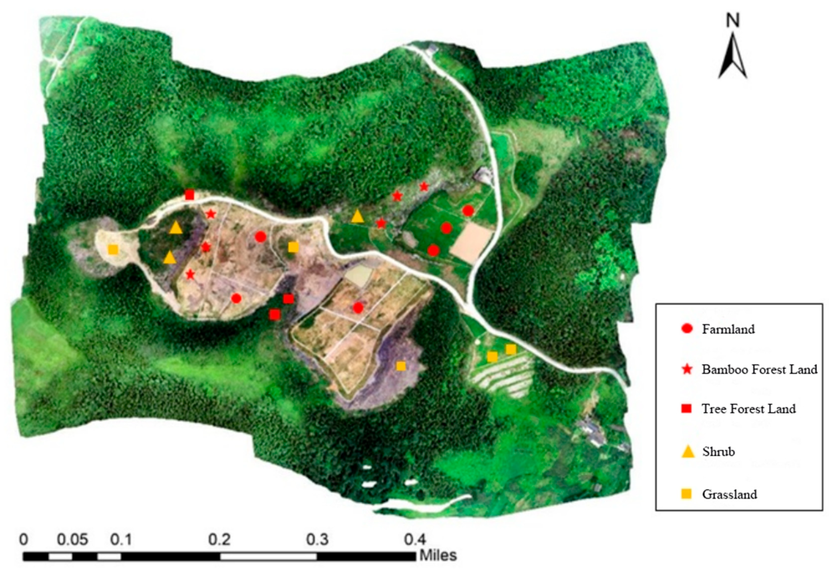
Total area of plots	3.8609	12.3623

), including dry land, arbor forest land, bamboo forest land, shrub land, grassland, and other areas. These areas had high ecological carbon sink benefits and were key areas in the carbon sink accounting, with survey plots set up for each type of land use according to the above formula. At the same time, the land also included paddy fields, agricultural land facilities, bare land, and other areas. Since the land functions of these areas were mainly for production, the ecological benefits were small and did not meet the requirements for carbon sink afforestation, so they were not considered in the accounting and no survey plots were set up.

The plots were located using GPS positioning, with the located points serving as the southwest corners of the plots, uniformly marked and numbered. Details of the survey plots are shown in the following table, and their distribution is shown in Figure 6.

The net carbon sink/source proportion was measured during the monitoring interval (within the time periods); when the calculation result was positive, the area was an absorption sink; if the calculation result was negative, it was an emission source. In this calculation, the start of the accounting period was the point before reclamation, and the end of the accounting period was the current survey point. By examining both early photos of the area and historical data collected on site, we found that the ecological degradation of the plot affected by mining was quite serious, with no effective soil layer on the surface and sporadic herbaceous plants, and it was considered to have a total carbon stock of zero at the beginning. The total carbon stock was the sum of the carbon storage in the carbon layer of each site targeted for restoration in the project area.

The results of the vegetation carbon sink accounting for abandoned mine pit X on Tongluo Mountain are shown in

Table 7. Total carbon sink values in the study area.

	Land Use Type	Area	Soil Carbon Stock	Vegetation Carbon Stock	Total Carbon Stock	Unit Area Carbon Sink Value
		ha	tC	tC	tC	tC/(ha·a)
Plot A	Arable land	2.2375	107.2192	0.7325	107.9517	48.247
	Arbor forest land	0	——	——	——	——
	Bamboo forest land	0.2626	14.2513	20.2488	34.5001	130.1379
	Shrubland	0.153	6.8781	6.1127	12.9908	84.907
	Grassland	0.599	12.7141	0.2828	12.9969	21.698
	Other	0.6088	——	——	——	——
	Total for Plot A	3.8609	141.0628	27.3768	168.4396	43.627
Plot B	Arable land	3.7268	109.6171	1.4127	111.0298	29.792
	Arbor forest land	2.2451	157.6060	1.2130	158.8190	70.740
	Bamboo forest land	0.5141	31.8351	27.6224	59.4575	115.654
	Shrubland	0.6640	46.4534	5.0990	51.5525	77.639
	Grassland	2.2741	193.2803	1.4223	194.7026	85.617
	Other	2.9382	——	——	——	——
	Total for Plot B	12.3623	538.7920	36.7694	575.5614	46.558

. The unit area vegetation carbon sink values of Plot A and Plot B in the study area were 7.091 tC/(ha·a) and 2.974 tC/(ha·a), respectively, and the total vegetation carbon reserves were 27.38 tC and 36.77 tC, respectively. The unit area soil carbon sink values of Plot A and Plot B in the study area were 36.536 tC/(ha·a) and 43.583 tC/(ha·a), respectively, and the total soil carbon reserves were 141.0628 tC and 538.7920 tC, respectively.

The sum of the soil carbon pool and vegetation carbon pool carbon reserves was obtained to obtain the total carbon reserve of the study area, and then the unit area carbon sink value was calculated, as shown in Table 7. The unit area carbon sink values of Plot A and Plot B were 43.6 tC/(ha·a) and 46.5 tC/(ha·a), respectively, and the total carbon reserves were 168.44 tC and 575.56 tC, respectively.

Considering the two major forms of carbon sinks, the main contribution to the carbon sink value of the mine ecological restoration came from the soil carbon sink; the unit area carbon sink value of the soil (40 tC/(ha·a)) was eight times that of the vegetation (5 tC/(ha·a)). Among the different land use types, there was a higher carbon sink value in the bamboo forest land, accounting for about 38% of the total unit carbon sink value.

In addition, when estimating the soil carbon reserves, our approach calculated the carbon stocks by multiplying the soil carbon density of different land types by their coverage area. It is important to note that the soil carbon density is often standardized based on a 1 m depth in many accounting methodologies, and this standard was utilized in the calculation of the density values for convenience in this study. However, in the restored mining areas of Tongluo Mountain, particularly at reclaimed sites, the actual soil cover thickness exhibits significant spatial heterogeneity and is typically much shallower, ranging from approximately 0.3–0.5 m for areas restored as forest land and farmland and 0.2–0.3 m for shrubland, based on field observations and restoration practices in the region. Due to this variability and the contrast between the actual depth of the reclaimed soil profiles and the 1 m standard, our current estimations may differ from the actual carbon stocks present in the soil. It is possible that relying on a density value standardized to a 1 m depth, while convenient, could lead to an overestimation compared to the total carbon contained within the actual, shallower soil profile at many sites. This spatial heterogeneity in the soil thickness suggests that the true soil carbon stocks across the restored areas could be lower than the calculated values if a uniform 1 m depth is assumed. However, even considering this potential variability and possible overestimation in specific localized areas, the calculated soil carbon stocks represent a substantial carbon pool within the overall restored mining landscape, highlighting its significant contribution to ecosystem carbon sequestration, particularly when compared to unmanaged sites.

5. Conclusions

This study makes a significant contribution by applying high-resolution GF-6 satellite imagery and ground data to assess the ecosystem carbon storage across different real-world restoration strategies in the complex, small-scale mining landscape of Tongluo Mountain, a representative karst area in southwest China. The research provides valuable insights into the comparative effectiveness of engineered restoration versus natural recovery and unmanaged closure for carbon sequestration in this specific context and highlights the potential of using China’s high-resolution satellite data for resource ecology applications.

Our findings demonstrate that engineered ecological restoration leads to a significantly higher aboveground biomass and overall carbon density (combining that of the vegetation and soil) compared to areas undergoing natural recovery or remaining unmanaged. This underscores the substantial benefits of active intervention in accelerating carbon recovery in degraded mining environments. While our model based on GF-6 indices showed a moderate correlation, indicating its potential utility for estimation, further improvements are needed for more precise quantification.

The analysis revealed that soil carbon constitutes a major component of the total carbon stock at these restored sites. Among the different vegetation types, certain species that were planted, notably in bamboo and arbor forests, exhibited high carbon sequestration potential, highlighting their importance in restoration planning in this region. Based on these results, we conclude the following:

(1)

Engineered ecological restoration is a highly effective strategy for significantly enhancing the carbon storage in mining areas like Tongluo Mountain compared to that achieved with natural recovery or at unmanaged sites.

(2)

Strategic vegetation selection is crucial, requiring a balance between a high carbon storage potential and suitability for challenging mine site conditions.

(3)

Prioritizing soil restoration practices is essential for increasing the soil carbon pool.

This study provides a scientific basis for policies that prioritize engineered restoration, guide strategic implementation, and support monitoring for enhanced carbon sequestration and sustainable development in mining regions. In future research and practice, we recommend exploring the integration of multi-source remote sensing data, including from readily available sources like Landsat and Sentinel, with high-resolution data and advanced modeling techniques to improve the accuracy and reliability of carbon stock estimations across broader areas and over time. Longitudinal monitoring is also needed to understand the long-term recovery trajectories.