Abstract
In the context of climate change, surface urban heat islands (SUHIs) have become critical factors affecting the quality of the urban built environment. However, low-precision satellite thermal infrared remote sensing is suitable for urban scales but is insufficient to reveal the spatiotemporal distribution roles of surface heat islands at the neighborhood scale. This research takes the Sipailou Campus of Southeast University as an example and employs UAV thermal infrared imaging to acquire high-precision surface temperature data. It then systematically investigates the relationship and association mechanism between the surface urban heat island intensity (SUHII) and campus 2D/3D landscape configuration. The results indicate that the campus has a cooling effect during the daytime, with an average SUHII of −0.90 °C. It demonstrates the SUHII characteristics for campus land use types are as follows: SUHII_BD > SUHII_IS > SUHII_GS > SUHII_WB. Furthermore, the campus landscape has a significant hierarchical driving effect on SUHII, with the configuration of campus buildings and the impervious surface driving the strong heat island (SHI) and the 3D configuration and structure of greenspace dominantly strengthening the strong cool island (SCI). The overall design strategy of “two-dimensional priority, three-dimensional optimization” enables us to effectively mitigate the campus SUHII. This study reveals the spatiotemporal distribution characteristics of campus SUHII and the key influencing factors, and it also broadens the application of UAV thermal infrared imaging technology in the meso–micro-scale urban heat island assessment, providing suggestions for constructing a climate-adaptive urban landscape.
1. Introduction
As climate change intensifies and extreme heat events become increasingly more common, the urban heat island (UHI) effect has gradually emerged as a key issue in urban living in recent years. According to the Intergovernmental Panel on Climate Change (IPCC), 2024 marks the 13th consecutive year of record-breaking global high temperatures [1]. From a social and economic perspective, the urban heat island effect intensifies the risk of exposure and vulnerability, threatening citizens’ physical and mental health and property security [2,3]. Therefore, mitigating the impact of the UHI effect has become an effective measure to improve urban livability and boost the development of a sustainable urban built environment [4,5,6].
Previous studies have suggested that urban surface heat island (SUHI) refers to the higher surface temperatures observed in urban areas compared to adjacent suburban or rural zones. This phenomenon is mainly caused by variations in land use patterns and underlying surface types during the urbanization process, such as increased building density and proportion of impervious surfaces, reduced vegetation coverage, and increased artificial heat sources [7]. SUHI research can be traced back to the 1970s. With the advancement of satellite thermal infrared remote sensing technology (such as the application of MODIS, ASTER, Landsat 8 TIRS, and Sentinel series), SUHI research has made breakthroughs in spatial resolution, time series analysis, and quantitative measurement methods [8,9]. Although the low spatial resolution (e.g., spatial accuracy ≥30 m) and low temporal resolution of satellite remote sensing data make it suitable for SUHI assessment at the city scale, it is not suitable for high-precision monitoring of the surface thermal environment at the neighborhood scale. Recently, some researchers have proposed a variety of ground-based or near-ground thermal infrared remote sensing methods, including airborne platforms, rooftop fixed temperature instruments, mobile handheld devices, etc., to obtain thermal infrared image data with higher spatial resolution and better temporal timeliness [10,11]. It is worth noting that the application of a single measurement method is often limited by its measurement points, labor costs, and weather conditions, making it difficult to accurately verify the validity of the collected data. To this end, it is necessary to assess the surface temperature more accurately and robustly using multi-source thermal infrared imaging methods.
University campuses, as an essential component of the urban built environment, offer significant potential for reducing heat island effects while providing ecological services [12]. Existing studies have shown that the local thermal environment can be effectively regulated through the rational distribution of different types of land uses (such as buildings, green spaces, water bodies, and road systems). However, current research has predominantly concentrated on macro-scale SUHI mitigation strategies [13,14], while paying insufficient attention to the internal spatial distribution patterns of thermal environments at the neighborhood scale. In addition, some campus heat island studies concentrated more on the spatial distribution heterogeneity of the heat island effect, with less attention on a systematic description of its temporal dynamic change process, ignoring the evolution characteristics and response mechanism of the heat island intensity at different time scales [15]. Therefore, it is essential for climate response campus planning and design to clarify the spatiotemporal variation in the heat island on university campuses and to identify the typical landscape patterns that affect high-temperature and low-temperature areas.
Landscape 2D/3D patterns and SUHI are intimately associated at the neighborhood level [16,17]. Among the two-dimensional landscape indices, the landscape percentage (PLAND), patch density (PD), edge density (ED), and landscape shape index (LSI) play a vital role in the surface heat island effect [18]. In addition, studies have shown that three-dimensional landscape indicators such as building height (BH), canopy height (CH), building density (BD), floor area ratio (FAR), and sky view index (SVF) can accurately explain the changing pattern of urban heat island intensity [19]. Among them, the relative importance of the 2D landscape index is greater than that of the 3D index. However, some studies have reached conclusions that contradict or are contrary to the above points. For example, Liu and Wang et al. found that 3D landscape features, such as building volume density (BVD), have a greater influence on LST than 2D landscape configuration [20]. Guo and Wu et al. have validated the impact of three-dimensional building configuration on the diurnal LST variations [21]. These results show that the correlation between the 2D/3D landscape index and surface heat island and the robustness of its results remains to be tested.
To fill this gap, this study uses multi-source thermal infrared imaging technology integrated with multiple linear regression and a gradient boosting tree model to investigate the spatio-temporal distribution characteristics of SUHI intensity on university campuses and its dominant influencing factors. This study is organized as follows: Section 1 reviews the current status of meso–micro-scale surface heat island research based on thermal infrared remote sensing technology; Section 2 interprets the research object and campus 2D/3D landscape index, and it briefly introduces the surface temperature monitoring, data processing, surface heat island intensity assessment, and correlation analysis methods based on multi-source thermal infrared imaging technology; Section 3 explores the dynamic spatiotemporal distribution characteristics of campus SUHI intensity and evaluates its correlation and relative importance; Section 4 discusses the design strategies to improve the surface heat island and the application prospects of new technologies; and Section 5 presents the conclusions of this research.
2. Materials and Methods
As illustrated in Figure 1, this study primarily consists of the following four sections: (1) Extract the high-precision surface temperature data of university campuses at various time periods during the day and evaluate its surface heat island intensity utilizing multi-source thermal infrared imaging. (2) Construct the campus 2D/3D landscape index and examine the spatio-temporal distribution heterogeneity of campus surface urban heat island intensity (SUHII) and its 2D/3D landscape index distribution characteristics. (3) Investigate the influence of the campus 2D/3D landscape patterns on SUHII and forecast the contribution of indicators using gradient boosting tree machine learning, Pearson correlation analysis, and multivariate linear regression. (4) Compare the SUHII distribution characteristics at various periods and intensity levels and discuss the dominant factors affecting the daily variation in campus SUHII in summer, to then propose design strategies and suggestions for climate-responsive campus landscape optimization.
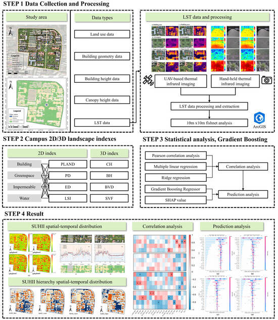
Figure 1.
Overall research framework proposed in this study.
2.1. Study Area
Nanjing is the capital of Jiangsu Province in eastern China, with a total area of 6587.04 square kilometers. It belongs to the subtropical humid monsoon climate zone with an average annual temperature of 17.6 °C. Recently, the meteorological records reveal an apparent warming trend, with summer temperatures reaching 31.3 °C in 2024. Therefore, it is necessary to mitigate the SUHI by optimizing the campus landscape design. Nanjing currently has more than 52 universities and 100 campuses, providing adequate research samples for urban heat island studies. In this research, we select the Sipailou Campus of Southeast University (longitude: 118.79, latitude: 32.05) as a representative case study in the metropolitan area, and its land use and spatial layout are shown in Figure 2. The total area of the campus is 41.1 hm2 and its high percentage of greenery (approximately 39%) has a potential cooling effect.
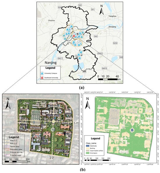
Figure 2.
Location of the study area. (a) Current research area and its corresponding remote sensing image; and (b) land cover types of the campus space, including buildings, impervious surfaces, greenspaces, and water bodies.
2.2. Data Collection
This study primarily employed the following observed and remote sensing data to quantify the campus surface heat island intensity: (1) Land use data. The 1 m resolution SinoLC-1 land use open-source data were extracted from Google Earth imagery and OpenStreetMap (OSM) data in December 2021 (https://doi.org/10.5281/zenodo.7707461), which include 11 land use types, such as tree cover, shrubland, grassland, building, traffic route, water, etc. In this study, the geographic information platform ArcGIS Pro is utilized to merge and reclassify them into the following four typical land use types: greenspace, building, water body, and impervious surface. (2) Building geometry and building height vector data. Based on Python 3.8, we crawled Baidu Map API (https://lbsyun.baidu.com/) and Amap API (https://lbs.amap.com/) to extract the shapefile vector data of the campus buildings. (3) Trees and plants. We conducted field surveys of the height and crown diameter of campus trees and plants in Appendix A Table A1 and cross-validated them with their location configuration on the campus CAD plan to ensure the accuracy and reliability of vegetation data. (4) Surface temperature data. We used multi-source thermal infrared imaging technology (e.g., airborne thermal infrared photography, handheld thermal infrared photography) to conduct field monitoring and obtain a 0.1 m resolution thermal infrared remote sensing image dataset from 1 July to 4 September 2024. Specific steps are described in Section 2.3.1. We used Pix4Dmapper software 4.9 and DJI Terra 3.7 to process the thermal infrared imagery and produce a series of campus LST maps. See Section 2.3.2 for specific procedures.
2.3. Methods
2.3.1. High Resolution Thermal Infrared Imaging
Referring to the multi-source thermal infrared measurement method [22,23], this study adopts a synchronous observation method, using UAV-mounted thermal infrared imaging system and a handheld thermal infrared radiometer to obtain highly accurate campus surface temperature data and perform cross-validation. The experimental procedure includes the following four main steps: (1) UAV-based thermal infrared image data acquisition; (2) handheld thermal infrared image data measurement; (3) surface temperature processing and extraction; and (4) emissivity correction and multi-source data registration.
This study used the following two thermal imagers: DJI Mavic 3T (airborne device) sourced from DJI (Shenzhen, China) and Testo-8751i Thermal Imager (handheld device) sourced from Testo SE & Co. KGaA (Titisee-Neustadt, Germany). Detailed device parameters and flight settings are shown in Table 1. The drone-mounted thermal imager was used for campus surface temperature monitoring and surface heat island (SUHI) calculation, while the handheld thermal imager was used for the comparison and calibration of the underlying campus surface emissivity.

Table 1.
Equipment specifications for DJI Mavic 3T and Testo-8751i Thermal Imager.
- (1)
- UAV-based thermal infrared imaging
This study conducted UAV-based thermal infrared imaging experiments at the Sipailou Campus of Southeast University from 1 July to 4 September 2024. The experimental weather conditions were selected to be cloudless and windless, with no water on the ground to ensure the accuracy of the thermal infrared data. In order to capture the dynamic changes in the surface heat island (SUHI) of the campus landscape on a typical summer day, the experiment set four time periods (8:00, 11:00, 14:00, and 18:00), covering the strongest and weakest periods of solar radiation, to analyze the evolutionary characteristics of the thermal environment at different time scales [24]. For the aerial surveys, we pre-planned flight paths based on the DJI Terra platform and set a fixed-route flight plan with a flight altitude of 120 m and ensured an 80% image overlap rate to improve data accuracy. Finally, 628 thermal infrared and RGB images were generated to establish a high temporal and spatial resolution dataset.
- (2)
- Handheld thermal infrared imaging
To enhance the reliability of airborne thermal infrared data, this study used the Testo-8751i handheld thermal infrared imager to perform synchronous ground temperature measurements for typical underlying surfaces [10]. Four major underlying surfaces (green spaces, buildings, impervious surfaces, and water bodies) were selected and six observation points were evenly distributed across the campus space (Figure 3). Due to differences in the thermal radiation characteristics of the underlying surface materials, a 30 cm × 30 cm aluminum foil panel was used as the calibration benchmark in this study. Since the reflectivity of aluminum foil is higher than 90% with stable thermal physical properties, the actual emissivity value of each material can be accurately calculated by synchronously measuring its temperature with different underlying surfaces. By calibrating the emissivity of the underlying surface, 30 JPG format thermal images were finally obtained. The radiation temperature was extracted by the Testo IRSoft 5.0 platform, and spatial statistical analysis was performed using ImageJ to obtain the average surface temperature data.
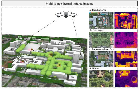
Figure 3.
Field measurements of campus surface temperatures across different land use types (e.g., green spaces, buildings, impervious surfaces, and water bodies) by using UAV-based thermal infrared imaging.
2.3.2. LST Processing and Extraction
- (1)
- Surface temperature conversion
The key to extracting LST data using UAV thermal infrared imaging is to convert RGB color values into surface temperature values containing location information. Firstly, we establish a mapping relationship between airborne thermal infrared images (JPG data) and surface temperature ranges. Then, Python is used to convert the pixel-by-pixel analysis of JPG format images and generate RAW format images containing temperature data, further converting them into TIFF format images for subsequent calculations (see Appendix B Figure A1). And the formula is listed as follows:
Secondly, we extract and supplement the POS location information of each image. As a professional drone aerial analysis software, Pix4DMapper can batch process thermal infrared images collected by drones and extract location information. Then, the original POS location information read by DJI Terra is imported into Pix4Dmapper software, thereby supplementing the precise location information such as geographic information, accuracy information, and heading angle. Third, we stitch the image. We input the TIFF format LST data and the edited POS location information into Pix4DMapper, and we use the image stitching function to generate a TIFF format image of the overall campus-built environment. The calculation process is shown in Figure 4.
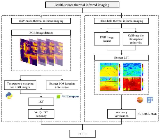
Figure 4.
Schematic diagram of the workflow for extracting and processing LST based on the thermal infrared imaging system carried by an unmanned aerial vehicle and a handheld thermal infrared radiometer.
- (2)
- Emissivity correction
The dominant factors that affect the accuracy of thermal infrared imaging mainly include the following aspects: (1) physical properties of the underlying surfaces and their surface emissivity; (2) meteorological conditions; and (3) UAV flight parameters. Among them, the surface emissivity is the most important influencing factor. In order to eliminate the influence of atmospheric absorption and scattering (including the absorption, scattering, and emission process of thermal infrared radiation by the atmosphere), this study uses the radiation transfer equation (RTE) to invert LST. The conventional RTE calculation formula is calculated as follows:
where ε is the target emissivity, τ represents the atmospheric transmittance, B(Ts) is the Planck radiation of the black body at the surface temperature, L↓ is the atmospheric downward radiation, and L↑ represents the upward radiation.
The emissivity measured by the drone is calibrated based on the surface temperature (Thandheld) and local emissivity (εhandheld) is measured by a handheld thermal infrared device. During the drone flight, the handheld imager is used to measure the surface temperature and its emissivity across four typical campus land use types (such as greenspace, building, impervious pavement, and water body) and record their coordinate positions. In summary, the corrected drone emissivity can be conducted by inverting the radiation transfer equation as follows:
Referring to Henn and Peduzzi [10], the calibrated surface temperature value is obtained by correcting the emissivity of different underlying surface types measured by the drone. The calculation equation is outlined as follows:
where Ts is the surface temperature and Trad is the radiation temperature.
- (3)
- Accuracy Verification
To prove the consistency of UAV and handheld thermal infrared image data, this study quantitatively analyzed the error levels of the two sets of data based on the coefficient of determination (R2), root mean square error (RMSE), and mean absolute error (MAE). The results showed that the mean R2 was 0.823, the mean RMSE was 2.36, and the MAE was 1.41 °C. Combining scatter plot analysis with the Bland–Altman test, it was found that the temperature difference was mainly distributed within the range of ±2.3 °C within the 95% confidence interval, which met the accuracy requirements of urban thermal environment research. Therefore, the applicability of UAV thermal infrared remote sensing in micro-scale surface temperature measurement was confirmed by establishing an air-ground integrated cross-validation system.
2.3.3. Campus 2D/3D Landscape Indicators
Two-dimensional and three-dimensional landscape indicators are often utilized to analyze the spatial structure and configuration characteristics of urban landscape environments [9,13,25]. Considering the synergistic effects of land use and landscape configuration on SUHI, this study selected 16 typical 2D landscape indices, covering four typical land use types as follows: building, greenspace, impervious surface, and water body. These indicators were used to quantify both the proportional composition and spatial configuration characteristics of campus landscapes. In detail, they included coverage-related metrics (e.g., percentage of landscape (PLAND) for buildings (PLAND_BD), greenspace (PLAND_GS), impervious surfaces (PLAND_IS), and water bodies (PLAND_WB)) and configuration metrics (e.g., PD_BD, ED_BD, LSI_BD, PD_GS, ED_GS, LSIS_GS, PD_IS, ED_IS, LSI_IS, PD_WB, ED_WB, LSI_WB). In addition, four 3D landscape indexes (including canopy height (CH), building height (BH), building volume density (BVD), and sky view factor (SVF)) were introduced to more comprehensively reflect the three-dimensional pattern characteristics of the campus landscape (Table 2). In this paper, a 10 m × 10 m grid fishnet analysis was conducted in ArcGIS Pro 3.3 and we used partition statistics table and range summary tools to calculate the campus 2D/3D landscape characteristics in each grid.
Table 2.
Campus 2D/3D landscape indexes.
2.3.4. Evaluation of Surface Urban Heat Island
Surface urban heat island intensity (SUHII) is a commonly adopted metric for assessing the surface heat island effect [30,31], and it has been extensively applied in urban thermal environment studies. SUHII is normally defined as the difference between urban surfaces temperature and their surrounding rural areas [32,33,34]. However, this measurement method based on urban–rural comparison is mainly applicable to the assessment of heat island effects at the macro or urban scale. In micro-scale research, the traditional urban–rural dichotomy is not fully applicable due to the heterogeneity of land use types and the local thermal environment. In particular, if the reference area is defined in different ways, the calculation results of the SUHII will be quite different. Referring to relevant literature [35,36], this study takes the average temperature of the campus and its surrounding 500 m buffer zone as the reference area. Then, the neighborhood-scale SUHII is redefined as the difference between the LST of a specific unit in the study area and the reference area. The calculation formula of the SUHII is outlined as follows:
where SUHIIi means the surface urban heat island intensity of the pixel i, indicating how much higher the pixel is than the mean temperature; LSTi is the surface temperature of the pixel i; is the average surface temperature; k is a correction term for background temperature fluctuations to avoid overestimating the heat island effect under the influence of factors such as green space and buildings. In this study, k is set to 0.5; Sd is the standard deviation of the surface temperature.
This study uses the raster calculator and focal statistics tools in the ArcGIS Pro platform to perform spatial smoothing on the SUHII data to eliminate the interference of extreme cold and heat sources on the temperature threshold. After processing, it seems that the SUHII fluctuation amplitude in the four observation periods is less than 30 °C. This result is consistent with the research conclusions of Ahmad and Eisma et al. on the fluctuation characteristics of SUHII at the urban neighborhood scale in summer [37], confirming its validity in urban heat island studies.
Furthermore, the SUHII classification is performed using the standard deviation method based on the ArcGIS Pro 3.3 platform. This approach statistically determines classification thresholds by analyzing the discrete degree of SUHII distribution, which is suitable for continuous datasets [38,39]. Otherwise, there exists a cool island effect, especially in campus vegetation and water coverage areas. Accordingly, the campus SUHII is divided into five categories as follows: strong heat island (SHI), weak heat island (WHI), no heat island (NHI), weak cool island (WCI), and strong cool island (SCI). In particular, the specific thresholds are shown in Table 3:
Table 3.
Threshold classification role for campus SUHII.
2.3.5. Statistical Analysis, Gradient Boosting, and SHAP Model
To investigate the relationships between campus 2D/3D landscape variables and SUHII variations, this study first employs the Pearson correlation coefficient to assess potential linear associations. Furthermore, multiple linear regression (MLR) and ridge regression (RG) models are utilized to examine the underlying influencing mechanisms. When the Pearson correlation coefficient (r) approaches ±1, it reflects a stronger linear dependence between the variables. However, Pearson analysis can only reflect the linear relationship between variables, and some studies have suggested that the impact of landscape configurations on surface temperature and surface heat island often involves the interaction of multiple factors [40]. Therefore, this study adopts multivariate linear regression and brings in ridge regression to eliminate the multicollinearity between partial indexes. Compared with the ordinary least squares method (OLS), ridge regression analysis uses biased estimation to build a more realistic regression model and improve its robustness. During this process, we introduce k unit matrices into the regression equation and screen the optimal K value. This ensures that the model avoids excessive bias while reducing variance, thereby more accurately revealing the driving mechanism of the campus-built environment on SUHII. The calculation equation of the ridge regression model is shown as follows:
where Y is the dependent variable, representing the SUHII value at different time period; X is the independent variable, representing the campus 2D/3D landscape index; n is the number of independent variables; and β represents the regression coefficient Beta of each variable calculated by ridge regression.
The gradient boosting regressor (GBR) model based on the gradient boosting tree is commonly adopted to quantify the contribution of the landscape indicators to the urban heat island [41]. Compared to algorithmic models such as XGBoost (XGB), the GBR shows high computational efficiency in small- and medium-sized datasets. The GBR-free model can prevent overfitting through its built-in tools assessing feature importance and interpretability, and it does not require explicit regularization, making it suitable for limited sample training [42]. Prior to model training, data preprocessing is required to clean the data and to standardize or normalize missing value imputation. The maximum depth of the tree is limited to 3, and the minimum number of samples for node splitting is set to 2 to avoid overfitting the GBR model.
Finally, SHAP is applied to quantify the marginal contribution of each feature to the predicted value across all feature combinations, offering a globally interpretable framework. The Shapley value is a method from coalitional game theory [43] and the Shapley value represents the contribution of an individual feature by averaging its impact over all possible subsets of features. This method is frequently used to interpret machine learning outputs and assess the relative importance of predictors in relation to the target variable [44,45]. In this study, we use the SHAP summary_plot and Feature Importance to illustrate the global importance of campus landscape indices, thereby interpreting the factors that influence the intensity of the campus surface heat island. The calculation equation is as follows:
where φi is the indicator attribute value, M is the number of input independent variables, N is the set of all input dependent variables, and φi ∈ R.
3. Results
3.1. Verification of UAV and Handheld Thermal Infrared Imaging
As shown in Table 4, the accuracy of UAV-based thermal infrared imaging technology is evaluated by comparing the LST measurements from airborne thermal infrared cameras and handheld thermal infrared devices. The results illustrate that the LST recorded in campus buildings, impervious pavement, and water body areas are generally consistent, exhibiting an average LST deviation of approximately 2 °C. This finding is supported by Kalogeropoulos and Tzortzi et al. [45], which suggested that the measured temperature for the underlying surface with stable emissivity characteristics is not affected by the sensor type. However, significant temperature differences appeared in the greenspace coverage area, with an average temperature difference of 6.13 °C. This high heterogeneity may be caused by the impact of building and tree shading effects on the land surface temperature.
Table 4.
Surface temperatures of campus landscape environments measured by UAV-based thermal infrared camera and handheld thermal imagers.
This study further selected typical underlying surface samples and systematically evaluated the consistency of UAV thermal infrared imaging and handheld measurement by using indicators such as R2, RMSE, and MAE. Figure 5 displays that the two measurement methods have a significant correlation at a 99% confidence level with Pearson correlation coefficient r = 0.946, R2 = 0.895, RMSE = 1.361 °C, and MSE = 1.852 °C. The error level of this study fully meets the requirements for high-precision measurement (RMSE ≤ 1.5 °C), which verifies the reliability of UAV thermal infrared imaging technology in quantitatively inverting LST.
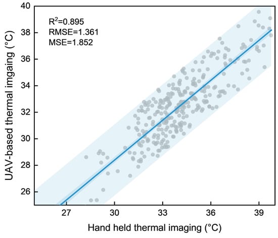
Figure 5.
Fitting regression analysis of UAV-based thermal infrared imagery and handheld thermal infrared imagery.
3.2. Characteristics of SUHII Spatiotemporal Distribution SUHII
3.2.1. SUHII Spatiotemporal Distribution
Figure 6a shows that the intensity and spatial distribution of the surface heat island of the campus landscape varies significantly over time. In general, SUHII_14:00 > SUHII_17:00 > SUHII_8:00 > SUHII_11:00, with mean values of 2.783 °C, −0.844 °C, −0.853 °C, and −1.806 °C, respectively. The results suggest that SUHII rises along with the increase in solar radiation and it reaches a peak in the afternoon at 14pm. In the early morning, the total intensity of the surface heat island and cold island is not high, and the spatial distribution difference is small, with a mean and standard deviation of −2.237 °C and 4.475 °C, respectively. At the dust, the intensity of the surface heat island and the cool island both declined. Different from the morning, impermeable surface areas continue to absorb heat during the day and become a major heat source contributing to the surface heat island.
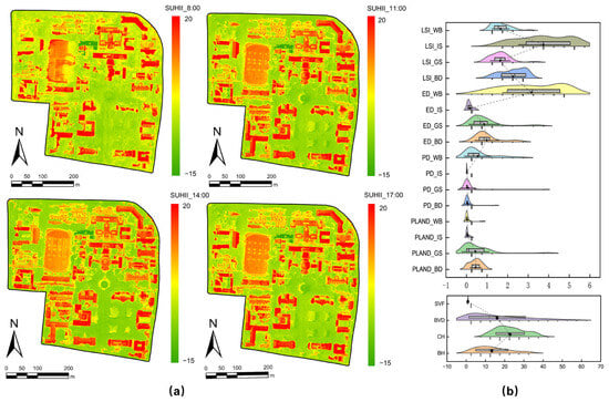
Figure 6.
Spatial distribution of SUHII in the study area. (a) The spatiotemporal distribution variations in SUHII in four typical time periods: 8:00, 11:00, 14:00, and 17:00. (b) The SUHII distribution range of campus 2D/3D landscape index.
Figure 6b illustrates the distribution characteristics of the campus 2D/3D landscape indexes. The results show that the campus landscape proportion (PLAND) from high to low as follows: PLAND_BD > PLAND_GS > PLAND_IS > PLAND_WB, with average values of 44.75%, 43.41%, 5.67%, and 3.83%, respectively. It means that campus building elements and greenspace coverage account for a higher proportion than other land use types. For the landscape complexity index, the result demonstrates that LSI_IS > LSI_BD > LSI_WB > LSI_GS, indicating that the campus impervious surface (such as roads, parking lots, and scattered hardened ground) presents a highly irregular edge morphology, while the campus green space has the lowest degree of spatial fragmentation. Furthermore, the ED_BD value is the highest, reflecting the complex morphology of building patches, which are normally small in size, and dispersed in campus space with diverse geometric shapes. And the ED_GS value ranks second, indicating that the greenspace distribution is moderately fragmented. On the other hand, the overall campus BH is lower than the CH, with an average value of approximately 22.84 m and 13.33 m. It is worth noting that the average SVF of the campus is approximately 0.78, which means that most of the campus landscape spaces are relatively open.
3.2.2. SUHII Hierarchy and Its Spatiotemporal Distribution
For the characteristics of SUHII hierarchy distribution, Figure 7a illustrates that the strong heat island and strong cool island areas change most significantly over time. At 8:00, the strong heat island areas are mostly scattered in the campus buildings and impervious pavement areas, and the strong cool island is located in the densely green coverage area and its shadow range. At 14:00, the strong and weak heat islands further expanded to the vicinity of buildings and impermeable pavement, and the strong cold islands were concentrated in vegetation and water areas. At 17:00, the strong cool island patches were densely distributed in large grass areas and tall tree areas, while the proportion of impermeable surfaces in the strong heat island areas increased significantly. Figure 7b suggests that campus buildings predominantly contribute 77.55% to the enhancement of the heat island effect, impervious surfaces contribute 15.31%, and greenspace contributes 83.52% to the enhancement of the cold island effect. When the solar radiation is strongest in the afternoon, campus buildings are the leading factors in both strong and weak heat islands, accounting for 95.88% and 68.89%, respectively. Greenspaces have the most prominent influence on strong and weak cool islands, accounting for 97.40% and 99.07%, respectively. Otherwise, after a whole day of solar radiation, the influence of campus greenspace and impermeable surface on the SUHI effect gradually reaches its highest at 17:00, accounting for 31.50% and 40.22%, respectively.
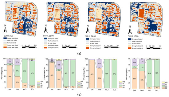
Figure 7.
SUHI intensity classification and categorization during the day. (a) Spatial and temporal heterogeneity of SUHII classification. (b) Land use proportion under different SUHII levels.
Figure 8 reveals significant differences in the temporal heterogeneity of SUHII under different land use types. Overall, the surface heat island or cool island effect reaches its peak at around noon. Among them, the distribution curve of the SUHII of the impervious surface area shows an inverted U-shaped curve, with the peak point appearing at 14:00, indicating that the impact of impervious surface on SUHI intensity first increased and then weakened. Although the building area exhibits a similar growth trend, the fluctuation amplitude is about 0.728 °C lower than that of the impermeable surface, showing a more stable thermal characteristic. Meanwhile, the SUHII variations in the green area and water area demonstrate a U-shaped curve, performing the peak cooling effect at midday with median SUHII values of −8.304 °C and −7.754 °C, respectively. Although the water body exhibits strong local cooling efficiency. Their limited spatial coverage (merely 1.02% of the campus area) significantly constrains the cumulative heat mitigation potential.
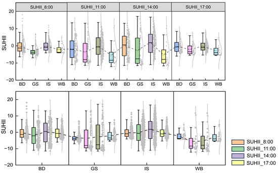
Figure 8.
SUHII temporal distribution of different land coverage.
3.2.3. Axis Analysis
To intuitively compare the spatial patterns of the SUHII, we conduct a comparative analysis of the thermal distribution profiles along representative horizontal and vertical axes in Figure 9. The results reveal distinct thermal characteristics between different landscape configurations. Figure 9a represents the campus landscape space with highly heterogeneous land use, where the SUHII curve demonstrates the obvious fluctuation characteristics, with the maximum fluctuation amplitude reaching 20.57 °C. Figure 9b reflects the campus landscape space with clear land use distinctions. And the SUHII between different functional areas is significantly different, while the SUHII within the same functional area remains relatively stable (such as the SUHII fluctuation range less than 2 °C). It is worth noting that the mean SUHII values of the two profile axes are −1.26 °C and −1.79 °C, respectively, suggesting that the whole campus is a weak cool island. This phenomenon is likely attributed to its high vegetation cover (39%) and the optimal spatial configuration of green and the spatial configuration of the green–blue infrastructure.
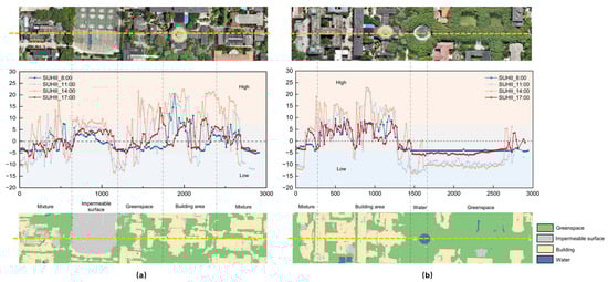
Figure 9.
Axis analysis of the SUHII spatial-temporal distribution of the campus-built environment. (a) SUHII distribution on the horizontal axis; (b) SUHII distribution on the vertical axis.
3.3. Correlation Between SUHII and Campus 2D/3D Landscape Indicators
3.3.1. Correlation Between the Campus 2D/3D Landscape Index and SUHII Spatiotemporal Distribution
In this study, the Pearson correlation analysis is adopted to identify campus landscape indicators that are significantly correlated with multi-temporal SUHII. Figure 10 illustrates the substantial correlation between SUHII and two-dimensional indices, including PLAND_BD, PD_BD, ED_BD, PLAND_GS, LSI_IS, and PLAND_WB. Among them, PLAND_BD and LSI_IS are positively correlated with SUHII, with correlation indexes of 0.846 and 0.490. However, SUHII had a negative association with PD_BD, ED_BD, PLAND_GS, and PLAND_WB, with correlation indices of −0.507, −0.549, −0.733, and −0.354, respectively. Conversely, there is a weak link between SUHII and the 3D indices represented by CH, BVD, and SVF, with correlation values of −0.450, 0.451, and −0.185, respectively. During the day, the correlation degree between campus landscape configuration and SUHII reached the highest level at 14:00, which is higher than other periods. Notably, the 2D indexes for campus greenspace and impervious surface landscape layout, such as PD_GS, ED_GS, LSI_GS, PD_IS, and ED_IS, showed correlation with SUHII at 14:00, but not at other periods.
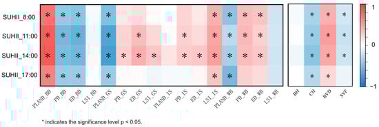
Figure 10.
Overview of the correlation between campus 2D/3D landscape and SUHII spatiotemporal distribution.
The results of multiple linear regression demonstrate that the campus 2D/3D landscape index generally fits well with the regression models of SUHII_8:00, SUHII_11:00, SUHII_14:00, and SUHII_17:00, with R2 of 0.807, 0.917, 0.967, and 0.869, respectively. However, the variance inflation factor (VIF) of PLAND_BD, PLAND_GS, PLAND_IS, and ED_IS is much greater than 10, and the tolerance is less than 0.1, indicating that there is significant collinearity between the above indices. Therefore, this study uses ridge regression analysis to further explain the impact of the campus landscape index on the spatiotemporal changes in SUHII.
Through ridge regression analysis, Table 5 displays the correlation between SUHII and the selected campus 2D/3D landscape index. The result shows that the above index has a strong significance for SUHII, because the significance of all periods SUHII_8:00, SUHII_11:00, SUHII_14:00, and SUHII_17:00 is less than 0.005 (all significance is 0.000). In each period, the goodness of the ridge regression model is very ideal, and the explanatory power of each variable on the dependent variable is 60.5%, 84.0%, 90.3%, and 58.0%, respectively. By comparing the standardized regression coefficient Beta, the regression coefficient after removing the unit effect of the independent and dependent variables can be obtained. The results display that PLAND_GS (Beta = −0.360), ED_BD (Beta = −0.095), CH (Beta = −0.064), and LSI_BD (−0.056) had a significant negative correlation with SUHII, while PLAND_BD (Beta = 0.359), ED_GS (Beta = 0.066), and BVD (Beta = 0.062) had a positive correlation with SUHII. These findings demonstrate that campus building and greenspace layout have a dominant influence on the spatiotemporal dynamics of SUHII.
Table 5.
Multiple linear regression analysis of the typical 2D/3D landscape index of campus and SUHII at different time periods.
3.3.2. Correlation of the Campus 2D/3D Landscape Index and SUHI Intensity Level
Figure 11 reveals the spatiotemporal correlation characteristics between the campus 2D/3D landscape and the surface heat island intensity (SUHII) hierarchy. The study shows a clear spatiotemporal distinction in the impact of the campus landscape index on SUHII; among them, the correlation between 14:00 and 17:00 is particularly significant. At 8:00, the 3D landscape index has the most prominent explanatory power for SUHII. Specifically, BH (r = 0.697) and SVF (r = 0.670) are significantly positively correlated with the weak heat island effect, while BVD (r = −0.611) is negatively correlated. It is worthwhile to note that the canopy height (CH, r = 0.675) has a significant contribution to the formation of the strong cold island effect (p < 0.05). At 14:00, the campus two-dimensional landscape index had a substantially higher explanatory power for SUHII than the three-dimensional index. Among them, the patch density (PD_BD, r = 0.704) and edge density (ED_BD, r = 0.649) of building land is strongly positively correlated with the cold island effect, while the contribution of green space proportion and impervious surface proportion is relatively weak. At 17:00, the campus landscape pattern index has the most significant impact on the enhancement of the heat island. LSI_BD, ED_GS, LSI_GS, and PLAND_IS are all positively correlated with the enhancement of the heat island effect. By contrast, BH (r = 0.797) and CH (r = 0.615) have a peak strengthening effect on the cold island effect.
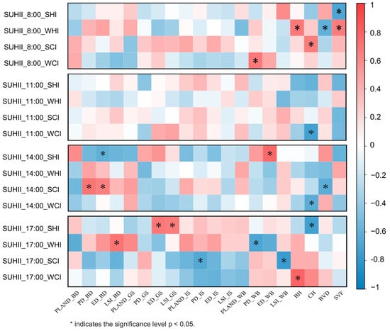
Figure 11.
Correlation between campus 2D/3D landscape and strong heat island (SHI), weak heat island (WHI), weak cold island (WCI), and strong cold island (SCI).
Through multivariate linear regression analysis (MLR), this study quantifies the differential driving effect of the multidimensional campus landscape index on the SUHII and its hierarchy (Table 6). Through multivariate linear regression analysis (MLR), this study quantified the differential driving effect of the multidimensional campus landscape index on the level of surface heat island intensity (SUHII). The model diagnosis showed that the variance inflation factor of all predictors is less than 10 (ranging from 2.474 to 9.700), and the tolerance (Tolerance) is more than 0.1 (ranging from 0.107 to 0.353), indicating that there is no significant multicollinearity problem and the model meets the statistical assumptions. The magnitude of the heat island effect is primarily regulated by the 2D landscape pattern, such as strong heat islands and weak heat islands.
Table 6.
Multiple linear regression analysis of campus 2D/3D landscape indicators and SUHII levels.
In particular, building edge density (ED_BD, β = −0.534), green patch density (PD_GS, β = −0.497), the impervious surface landscape shape index (LSI_IS, β = −0.338), and green edge density (ED_GS, β = −0.102) are all significantly negatively correlated with the strong heat island (p < 0.05, p < 0.001), suggesting a significant inhibitory effect on the heat island. However, 3D landscape indicators mostly impact the cool island levels, which include the weak cool island and strong cool island. Specifically, canopy height (CH, β = 1.068) significantly promotes the formation of cool islands. While the sky view factor (SVF, β = −1.134) and building volume density (BVD, β = −1.111) showed significant negative contributions.
3.4. Predicting the Contribution of Campus 2D/3D Landscape Patterns to SUHII
In this study, the spatial distribution of campus 2D/3D landscape data and SUHII data are integrated into a continuous dataset containing 470 samples, divided into 80% training and 20% test samples to ensure the independence of model evaluation. As shown in Table 7, there are significant differences in the prediction performance of the GBR model at different periods. For instance, the average determination coefficient (R2) of the training set and the test set have reached 0.957 and 0.773, respectively. It demonstrates that the model still has a strong explanatory power in retaining sample data. Moreover, the GBR model has the best prediction performance at 14:00, with test set R2 = 0.989. This phenomenon demonstrates that the prediction ability of the GBR model will increase along with SUHI intensity.
Table 7.
Prediction accuracy of the GBR model on the relative importance of campus 2D/3D landscape indicators to SUHII.
As shown in Figure 12, this study systematically evaluates the predicted contribution of 20 campus landscape indices to the SUHII by integrating global feature importance and SHAP bee swarm plots. The mean |SHAP value| at the X-axis reflects the absolute contribution of each index to the SUHII prediction, and the Y-axis ranks them according to their relative importance. With red representing a strong contribution and blue representing a low contribution, the gradient shift from red to blue illustrates the shift in the strength of the characteristic value’s influence on SUHII.
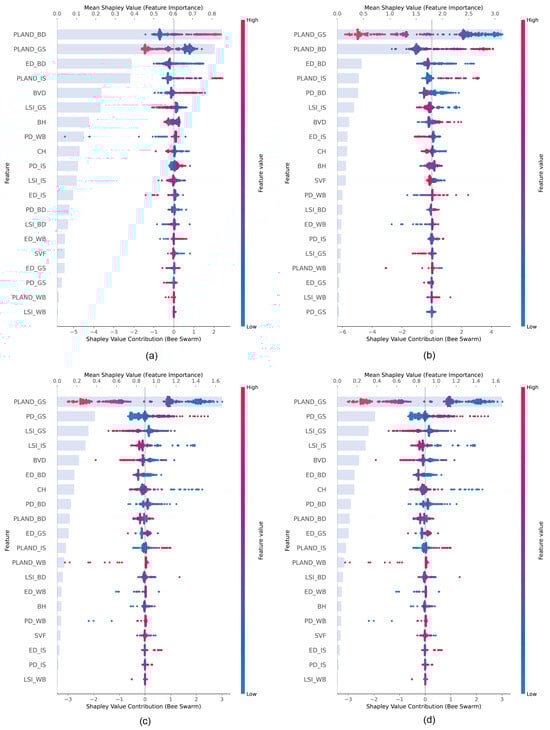
Figure 12.
Relative importance of the 2D/3D landscape indexes to SUHII. (a) Relative importance at 8:00. (b) Relative importance at 11:00. (c) Relative importance at 14:00. (d) Relative importance at 17:00.
The results suggest that there are notable differences in the distribution features of feature importance in different periods. In general, high SHAP scores are mostly distributed at the greenspace, building, and impervious surface coverage areas. Among them, PLAND_BD, PLAND_IS, and PD_GS are positively correlated with SUHII, while PLAND_GS, LSI_GS, and LSI_IS are negatively correlated. For the characteristics of color distribution, the red value range of the PLAND_BD, PLAND_IS, and BVD indices is broadly distributed and exhibits a monotonically increasing tendency. In summary, the significance of indices such as PLAND_GS, PD_GS, LSI_GS, and LSI_IS are gradually improved from 8:00 to 17:00. More specifically, the high and low SHAP values of PLAND_GS are broadly distributed in both positive and negative regions, suggesting that the impact on SUHII is highly dependent on the interaction of other features or the local environment. The high SHAP values of PD_GS are discretely distributed and the low SHAP values are compactly distributed in the negative region, indicating that PD_GS exhibits a consistent negative contribution to SUHII and is context dependent. On the contrary, LSI_GS has a stable negative contribution. On the other hand, 3D landscape indicators like CH, BH, and SVF typically have low SHAP values, illustrating that these indicators have weak independent explanatory power for SUHII. In conclusion, there exists a scale effect for the contribution of the campus landscape index to SUHII.
4. Discussion
4.1. Applicability of High-Precision Thermal Infrared Remote Sensing in Surface Urban Heat Island Research
Current research demonstrates that multi-source thermal infrared imaging data (including satellite imagery, fixed cameras, and airborne and handheld thermal devices) have been widely applied in land surface temperature (LST) and surface urban heat island (SUHI) studies [46]. However, there is a significant gap in understanding the dynamic mechanisms and driving factors of surface urban heat island intensity (SUHII) at neighborhood scales. In particular, it lacks systematic analyses based on high-precision thermal infrared imaging. To address this point, this study innovatively employs a UAV-based thermal infrared device to acquire continuous LST data with hourly time resolution and ultra-high spatial resolution (up to 0.05 m), and it uses cross-validation with handheld thermal measurements to confirm data reliability and methodological effectiveness.
Compared to the conventional 30 m resolution satellite data, the high-precision UAV-based thermal infrared imaging technology enables the accurate quantification and spatial identification of the surface heat island effect for micro-scale land use types (such as building, greenspace, impermeable surface, water body, etc.). Integrated with the gradient-boosted regression tree model (GBR), the prediction accuracy for the SUHII is estimated to be 96.7%. Notably, the airborne thermal infrared technology effectively overcomes the limitations of satellite remote sensing for local-scale studies, successfully capturing diurnal SUHII variations and key drivers of extreme heat island or cool island phenomena. Through the 10m-grid analysis, the study further explores the relationship between 2D/3D landscape configurations and surface heat islands, establishing a new research paradigm and data foundation for urban thermal environment optimization.
4.2. Key Factors Affecting the Campus
The formation of SUHII heterogeneity in meso-scale and micro-scale urban landscape environments is relatively complex and is usually affected by the superposition of factors such as land use type, 2D/3D landscape pattern, and meteorological conditions. By exploring the correlation between campus land use and SUHII spatiotemporal heterogeneity and its intensity heterogeneity, we find that campus buildings and greenspace are the main factors affecting SUHII. Buildings and impervious surfaces are significantly correlated with the intensification of heat island effects, while green spaces and water bodies are positively correlated with cool island effects. These findings have been confirmed in previous research on urban thermal environments [47]. Furthermore, the land use pattern of the campus directly influences surface heat island intensity, with mixed-use areas exhibiting dramatic SUHII fluctuations. Meanwhile, the SUHII in a single land use area remains relatively constant, with a range of variation of less than 2 °C. This difference highlights the critical role of land use homogeneity in moderating microclimate variability within local thermal environments.
In addition, the study finds that the spatial layout of greenspace, buildings, and impervious surfaces contributes more significantly to SUHII. This conclusion is consistent with the conclusion of Mo and Huang et al. [20] that 2D morphological indicators dominate the urban surface temperature. As shown in Table 8, the campus 2D landscape index has a prediction accuracy of 90.8% for SUHII, while the contribution rate of the 3D landscape index is estimated to be only 39.2%. However, our findings partially contradict the points made by Luo and Yu et al., who highlighted the significant influence of three-dimensional green space characteristics on LST [9,15]. Our results show relatively low predictive values of building height for SUHII. This is probably due to the significant building height variation (coefficient of variation CV = 0.63), with high-rise and low-rise buildings coexisting, which may reduce the sensitivity of 3D features to SUHII. SVF, BVD, and CH exhibit strong correlations with both intense heat island and cool island effects, suggesting their critical role in modulating heat island phenomena within the campus environment.
Table 8.
Regression coefficients of all campus 2D/3D built environment indices on SUHII (=0.005).
4.3. Implications for Urban Planning and Design
As a significant part of the urban landscape environment, university campuses are the fundamental space for teachers and students studying and living. However, the association mechanism between their landscape characteristics and urban thermal environment has not been fully quantified. This paper analyzes the spatiotemporal variation in the campus surface urban heat island and finds that the average SUHII is mostly distributed around −0.90 °C. This finding reflects that there is a phenomenon of coexistence of local heat islands and cool islands in the campus environment. Compared with existing studies, it has demonstrated that the average cooling range of urban parks in summer was 2.22 °C [27], which further confirmed the cooling potential of the campus landscape as a cooling source.
Otherwise, the mean SUHII of campus greenspace and water area (SUHII = −4.05 °C) is significantly lower than the average for the overall campus landscape environment. This result indicates that a reasonable configuration of greenspace and water features can effectively alleviate the campus surface heat island effect. For instance, Xu and Sheng et al. confirmed that the integration of greenspaces and water bodies has a significant impact on the cooling effect in Nanjing [48]. Furthermore, Bai and Wang et al. further pointed out that the compact layout of three-dimensional greenspace can maximize its cooling effect [15]. Above all, optimizing the three-dimensional spatial configuration of campus green spaces and water bodies is expected to significantly adjust the campus thermal environment. Accordingly, this study proposes the following optimization strategies for strengthening its cooling benefits and alleviating the urban heat island effect.
First, we recommend increasing the amount of green space and water coverage. Adopting the decentralized, high-density small green patches with increased edge density can maximize the cooling of the greenspace–building interface. Second, we suggest optimizing the building–green space coordination. It should avoid the concentrated impervious surfaces while increasing the building patch and its edge density to promote interspersed layouts. Third, we propose strengthening three-dimensional landscape regulation. Using vertical greening (e.g., planting tall trees) combined with low-density building clusters can enhance their shading and evapotranspiration effects. Overall, campus landscape design should adopt a comprehensive planning strategy “2D prioritization, 3D optimization” that synergistically enhances both horizontal landscape configuration and vertical thermal regulation, aiming to adjust the campus thermal environment while effectively mitigating extreme urban heat and heat island pressures.
4.4. Limitations and Future Work
Although this study has verified the effectiveness of multi-source thermal infrared imaging in assessing the SUHII at the meso–micro-scale, it still has the following limitations: First, the current study primarily concentrates on the SUHII variations for the daytime and lacks a comparative analysis of the laws of SUHII changes between months, quarters, and seasons. In the future, it incorporates long-term meteorological monitoring data to reveal the dynamic response regulations of SUHII at different time scales (such as diurnal variations and seasonal transition periods), especially focusing on the triggering mechanism of extreme high-temperature events. Second, the scale effect and threshold of landscape indicators need to be further investigated. The following research can deeply explore the optimization thresholds and interactions of key indicators (such as green patch density and building volume density) and the non-linear relationship between 2D/3D landscape indicators and thermal environment and their marginal effects. In addition, it is possible to integrate satellite thermal infrared images (such as Landsat and Sentinel-3) with drone thermal infrared imaging data to construct the “macro–meso–micro” multi-scale analysis framework, thereby proposing more universal landscape design strategies.
5. Conclusions
By utilizing multi-source thermal infrared imaging technology, this study takes Southeast University’s Sipailou Campus as an example to investigate the correlation and mechanism between the spatiotemporal distribution of surface heat island intensity and the 2D/3D landscape patterns of university campuses. After analyzing the spatiotemporal distribution of SUHII, it classifies the campus SUHII into five hierarchies—strong heat island (SHI), weak heat island (WHI), no heat island (NHI), weak cold island (WCI), and strong cold island (SCI). Then, it mainly discusses the dominant influencing factors for strong heat islands and strong cold islands by employing multiple linear regression, ridge regression, and gradient-boosted regression tree models. The main findings are summarized as follows:
During the day, the campus landscape generally exhibits a cooling effect, with an average SUHII of −0.90 °C. From highest to lowest, the campus average SUHII is as follows: SUHII_BD > SUHII_IS > SUHII_GS > SUHII_WB, with a SUHII peaking maximum at 14:00. Secondly, the two-dimensional layout and configuration of campus buildings and impervious surfaces have become key factors driving the strong heat island effect. Campus building accounts for 77.55% of the SUHI intensity, whereas impervious surfaces account for 15.31%. Other than that, greenspace configuration and its 3D characteristics have emerged as important drivers of the substantial cool island effect, contributing 83.52% to the cool island. Thirdly, the campus 2D/3D landscape index has a significant hierarchical driving effect on the SUHII. The ED_BD, PD_GS, LSI_IS, and ED_GS are all significantly negatively correlated with the heat island benefit, indicating that there is an inhibitory effect on the strong heat island benefit. The CH is significantly positively correlated with the cold island, while the SVF and BVD show negative contributions.
In conclusion, a decentralized, high-density, small-patch greenspace and high-density building edges can enhance the cooling effect and mitigate strong heat island areas. In summary, this study takes campus landscape as the research object to explore the spatiotemporal variation in surface heat island intensity, broadening the application of multi-source high-precision thermal infrared imaging technology in evaluating SUHII at the micro-scale. Lastly, this study identifies the critical elements that significantly affect the SUHII and provides scientific support for the future optimization design of urban landscapes.
Author Contributions
Conceptualization, W.D. and J.W.; methodology, W.D.; validation, Y.Y. and S.S.; Visualization, W.D.; Writing—Original Draft, W.D.; Writing—Review and Editing, J.W.; Supervision, J.W.; Project administration, J.W. All authors have read and agreed to the published version of the manuscript.
Funding
This work was supported by the National Natural Science Foundation of China [grant number: 52078113].
Data Availability Statement
The data that support the findings of this study are available from the corresponding author upon reasonable request.
Acknowledgments
The authors would like to extend their gratitude to Peng Haolun of Nanjing University for the technical support.
Conflicts of Interest
The authors declare that there is no known competing financial interests or personal relationships that could have appeared to influence the work reported in this paper.
Abbreviations
The following abbreviations are used in this manuscript:
| UHI | Urban heat island |
| SUHI | Surface urban heat island |
| SUHII | Surface urban heat island intensity |
| MLR | Multivariate linear regression |
| OLS | Ordinary least squares |
| GBR | Gradient-boosted regression tree model |
| RG | Ridge regression |
| SHI | Strong heat island |
| WHI | Weak heat island |
| NHI | No heat island |
| SCI | Strong cool island |
| WCI | Weak cool island |
Appendix A
Table A1.
Statistics of typical vegetation information at the Sipailou Campus of Southeast University.
Table A1.
Statistics of typical vegetation information at the Sipailou Campus of Southeast University.
| No. | Name | Plant Families | Breast Height Diameter (cm) | Tree Height (m) | Crown Diameter (m) |
|---|---|---|---|---|---|
| 1 | Cinnamomumcamphora (L.) Presl | Lauraceae | 24.2 | 14.2 | 4.6 |
| 2 | Bischofia polycarpa (H.Lév.) Airy Shaw | Euphorbiaceae | 26.1 | 18.8 | 5.2 |
| 3 | Ligustrum lucidum Ait. | Oleaceae | 14.6 | 16.4 | 4.2 |
| 4 | Koelreuteriapaniculata | Sapindaceae | 18.7 | 15.6 | 5.0 |
| 5 | Acer palmatumThunb | Sapindaceae | 12.4 | 11.8 | 3.6 |
| 6 | Cerasusserrulata (Lindl.) Londonvar. lannesiana (Carri.) Makino | Rosaceae | 10.4 | 13.8 | 4.0 |
| 7 | GinkgobilobaL | Ginkgoaceae | 12.0 | 15.8 | 3.4 |
| 8 | Eriobotryajaponica | Rosaceae | 14.5 | 12.6 | 3.6 |
| 9 | MagnoliaGrandiflora Linn | Magnoliaceae | 14.3 | 12.8 | 3.8 |
| 10 | MalushallianaKoehne | Rosaceae | 10.8 | 13.2 | 2.8 |
Table A2.
Data statistics of the SUHII distribution for typical campus horizontal and vertical axes.
Table A2.
Data statistics of the SUHII distribution for typical campus horizontal and vertical axes.
| Axis 1-1 | Mean (°C) | Standard Deviation (°C) | Maximum (°C) | Minimum (°C) | Range (°C) |
|---|---|---|---|---|---|
| SUHII_8:00 | −1.03 | 4.72 | 21.27 | −7.09 | 28.36 |
| SUHII_11:00 | −0.72 | 8.69 | 18.00 | −16.98 | 34.98 |
| SUHII_14:00 | −0.46 | 9.62 | 17.94 | −19.27 | 37.21 |
| SUHII_17:00 | −0.35 | 4.36 | 13.62 | −13.62 | 27.24 |
| Axis 2-2 | Mean (°C) | Standard Deviation (°C) | Maximum (°C) | Minimum (°C) | Range (°C) |
| SUHII_8:00 | −2.28 | 4.72 | 9.68 | −6.90 | 16.58 |
| SUHII_11:00 | −4.90 | 9.97 | 19.04 | −16.51 | 35.55 |
| SUHII_14:00 | −6.28 | 10.90 | 18.27 | −19.11 | 37.38 |
| SUHII_17:00 | −2.36 | 4.60 | 8.24 | −7.34 | 15.58 |
Appendix B
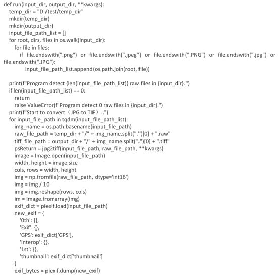
Figure A1.
Python-based UAV thermal infrared imaging data processing flow. This section focuses on one of the key steps—the conversion of thermal infrared images in RAW format to temperature TIFF data.
References
- United Nations. Climate Report. United Nations. Available online: https://www.un.org/en/climatechange/reports?gad_source=1&gclid=Cj0KCQjwxsm3BhDrARIsAMtVz6NYaKRMhM30OFkKx52uvqXLLij0Z6Qa6fIylZ5APkrtXbw7kv4MtdYaAkH-EALw_wcB (accessed on 24 September 2024).
- Dai, Y.; Liu, T. Spatiotemporal Mechanism of Urban Heat Island Effects on Human Health—Evidence from Tianjin City of China. Front. Ecol. Evol. 2022, 10, 1010400. [Google Scholar] [CrossRef]
- Deng, X.; Cao, Q.; Wang, L.; Wang, W.; Wang, S.; Wang, S.; Wang, L. Characterizing Urban Densification and Quantifying Its Effects on Urban Thermal Environments and Human Thermal Comfort. Landsc. Urban Plan. 2023, 237, 104803. [Google Scholar] [CrossRef]
- You, M.; Huang, J.; Guan, C. Are New Towns Prone to Urban Heat Island Effect? Implications for Planning Form and Function. Sustain. Cities Soc. 2023, 99, 104939. [Google Scholar] [CrossRef]
- Chandan, D.; Mark, R.; Nicholas, J.; Jane, P. Unlivable: What the Urban Heat Island Effect Means for East Asia’s Cities|GFDRR; World Bank: Washington, DC, USA, 2023. [Google Scholar]
- Gao, K.; Haddad, S.; Paolini, R.; Feng, J.; Altheeb, M.; Mogirah, A.A.; Moammar, A.B.; Santamouris, M. The Use of Green Infrastructure and Irrigation in the Mitigation of Urban Heat in a Desert City. Build. Simul. 2024, 17, 679–694. [Google Scholar] [CrossRef]
- Stewart, I.D.; Oke, T.R. Local Climate Zones for Urban Temperature Studies. Bull. Am. Meteorol. Soc. 2012, 93, 1879–1900. [Google Scholar] [CrossRef]
- Addas, A.; Goldblatt, R.; Rubinyi, S. Utilizing Remotely Sensed Observations to Estimate the Urban Heat Island Effect at a Local Scale: Case Study of a University Campus. Land 2020, 9, 191. [Google Scholar] [CrossRef]
- Luo, P.; Yu, B.; Li, P.; Liang, P.; Liang, Y.; Yang, L. How 2D and 3D Built Environments Impact Urban Surface Temperature under Extreme Heat: A Study in Chengdu, China. Build. Environ. 2023, 231, 110035. [Google Scholar] [CrossRef]
- Henn, K.A.; Peduzzi, A. Surface Heat Monitoring with High-Resolution UAV Thermal Imaging: Assessing Accuracy and Applications in Urban Environments. Remote Sens. 2024, 16, 930. [Google Scholar] [CrossRef]
- Lin, S.; Ramani, V.; Martin, M.; Arjunan, P.; Chong, A.; Biljecki, F.; Ignatius, M.; Poolla, K.; Miller, C. District-Scale Surface Temperatures Generated from High-Resolution Longitudinal Thermal Infrared Images. Sci. Data 2023, 10, 859. [Google Scholar] [CrossRef]
- Vanos, J.; Pfautsch, S. Building and School-Playground Design to Protect from Weather Extremes. In The Impact of Extreme Weather on School Education; Routledge: London, UK, 2023; pp. 94–118. [Google Scholar] [CrossRef]
- Qi, Y.; Chen, L.; Xu, J.; Liu, C.; Gao, W.; Miao, S. Influence of University Campus Spatial Morphology on Outdoor Thermal Environment: A Case Study from Eastern China. Energy Built Environ. 2023, 6, 43–56. [Google Scholar] [CrossRef]
- Ke, X.; Men, H.; Zhou, T.; Li, Z.; Zhu, F. Variance of the Impact of Urban Green Space on the Urban Heat Island Effect among Different Urban Functional Zones: A Case Study in Wuhan. Urban For. Urban Green. 2021, 62, 127159. [Google Scholar] [CrossRef]
- Bai, Y.; Wang, K.; Ren, Y.; Li, M.; Ji, R.; Wu, X.; Yan, H.; Lin, T.; Zhang, G.; Zhou, X.; et al. 3D Compact Form as the Key Role in the Cooling Effect of Greenspace Landscape Pattern. Ecol. Indic. 2024, 160, 111776. [Google Scholar] [CrossRef]
- Li, Y.; Schubert, S.; Kropp, J.P.; Rybski, D. On the Influence of Density and Morphology on the Urban Heat Island Intensity. Nat. Commun. 2020, 11, 2647. [Google Scholar] [CrossRef]
- Li, Z.; Hu, D. Exploring the Relationship between the 2D/3D Architectural Morphology and Urban Land Surface Temperature Based on a Boosted Regression Tree: A Case Study of Beijing, China. Sustain. Cities Soc. 2022, 78, 103392. [Google Scholar] [CrossRef]
- Khan, M.S.; Ullah, S.; Chen, L. Variations in Surface Urban Heat Island and Urban Cool Island Intensity: A Review Across Major Climate Zones. Chin. Geogr. Sci. 2023, 33, 983–1000. [Google Scholar] [CrossRef]
- Wu, W.-B.; Yu, Z.-W.; Ma, J.; Zhao, B. Quantifying the Influence of 2D and 3D Urban Morphology on the Thermal Environment across Climatic Zones. Landsc. Urban Plan. 2022, 226, 104499. [Google Scholar] [CrossRef]
- Mo, Y.; Huang, Y.; Zhong, R.; Wang, B.; Guo, Z. Investigating the Effects of 2D/3D Urban Morphology on Land Surface Temperature Using High-Resolution Remote Sensing Data. Buildings 2025, 15, 1256. [Google Scholar] [CrossRef]
- Liu, Y.; Wang, Z.; Liu, X.; Zhang, B. Complexity of the Relationship between 2D/3D Urban Morphology and the Land Surface Temperature: A Multiscale Perspective. Environ. Sci. Pollut. Res. 2021, 28, 66804–66818. [Google Scholar] [CrossRef]
- Guo, F.; Wu, Q.; Schlink, U. 3D Building Configuration as the Driver of Diurnal and Nocturnal Land Surface Temperatures: Application in Beijing’s Old City. Build. Environ. 2021, 206, 108354. [Google Scholar] [CrossRef]
- Rodríguez, M.V.; Melgar, S.G.; Márquez, J.M.A. Assessment of Aerial Thermography as a Method of in Situ Measurement of Radiant Heat Transfer in Urban Public Spaces. Sustain. Cities Soc. 2022, 87, 104228. [Google Scholar] [CrossRef]
- Fu, H.; Jiao, Y.; Deng, L.; Wang, W. Dynamic Impacts of Vegetation Growth and Urban Development on Microclimate and Building Energy Consumption. Sustain. Cities Soc. 2025, 126, 106382. [Google Scholar] [CrossRef]
- Hami, A.; Abdi, B. Students’ Landscaping Preferences for Open Spaces for Their Campus Environment. Indoor Built Environ. 2021, 30, 87–98. [Google Scholar] [CrossRef]
- Liu, Y.; Chen, C.; Li, J.; Chen, W.-Q. Characterizing Three Dimensional (3-D) Morphology of Residential Buildings by Landscape Metrics. Landsc. Ecol. 2020, 35, 2587–2599. [Google Scholar] [CrossRef]
- Han, D.; Xu, X.; Qiao, Z.; Wang, F.; Cai, H.; An, H.; Jia, K.; Liu, Y.; Sun, Z.; Wang, S.; et al. The Roles of Surrounding 2D/3D Landscapes in Park Cooling Effect: Analysis from Extreme Hot and Normal Weather Perspectives. Build. Environ. 2023, 231, 110053. [Google Scholar] [CrossRef]
- Han, D.; Cai, H.; Wang, F.; Wang, M.; Xu, X.; Qiao, Z.; An, H.; Liu, Y.; Jia, K.; Sun, Z.; et al. Understanding the Role of Urban Features in Land Surface Temperature at the Block Scale: A Diurnal Cycle Perspective. Sustain. Cities Soc. 2024, 111, 105588. [Google Scholar] [CrossRef]
- Yu, Q. Assessing the Cooling Effects of Urban Vegetation on Urban Heat Mitigation in Selected U.S. Cities. Master’s Thesis, University of South Florida, Tampa, FL, USA, 2018. Available online: https://digitalcommons.usf.edu/etd/8147 (accessed on 2 May 2025).
- Liu, L.; Zheng, B. Greenspace Coverage vs. Enhanced Vegetation Index: Correlations with Surface Urban Heat Island Intensity in Different Climate Zones. Urban Clim. 2024, 58, 102140. [Google Scholar] [CrossRef]
- Gage, E.A.; Cooper, D.J. Relationships between Landscape Pattern Metrics, Vertical Structure and Surface Urban Heat Island Formation in a Colorado Suburb. Urban Ecosyst. 2017, 20, 1229–1238. [Google Scholar] [CrossRef]
- Kim, S.W.; Brown, R.D. Urban Heat Island (UHI) Variations within a City Boundary: A Systematic Literature Review. Renew. Sustain. Energy Rev. 2021, 148, 111256. [Google Scholar] [CrossRef]
- He, B.-J. Towards the next Generation of Green Building for Urban Heat Island Mitigation: Zero UHI Impact Building. Sustain. Cities Soc. 2019, 50, 101647. [Google Scholar] [CrossRef]
- Oke, T.R. The Energetic Basis of the Urban Heat Island. Q. J. R. Meteorol. Soc. 1982, 108, 1–24. [Google Scholar] [CrossRef]
- Sobrino, J.A.; Irakulis, I. A Methodology for Comparing the Surface Urban Heat Island in Selected Urban Agglomerations Around the World from Sentinel-3 SLSTR Data. Remote Sens. 2020, 12, 2052. [Google Scholar] [CrossRef]
- Xu, Z.; Zhao, S. Scale Dependence of Urban Green Space Cooling Efficiency: A Case Study in Beijing Metropolitan Area. Sci. Total Environ. 2023, 898, 165563. [Google Scholar] [CrossRef]
- Zhang, J.; Tu, L.; Shi, B. Spatiotemporal Patterns of the Application of Surface Urban Heat Island Intensity Calculation Methods. Atmosphere 2023, 14, 1580. [Google Scholar] [CrossRef]
- Cai, X.; Yang, J.; Zhang, Y.; Xiao, X.; Xia, J. Cooling Island Effect in Urban Parks from the Perspective of Internal Park Landscape. Humanit. Soc. Sci. Commun. 2023, 10, 674. [Google Scholar] [CrossRef]
- Anjos, M.; Lopes, A. Urban Heat Island and Park Cool Island Intensities in the Coastal City of Aracaju, North-Eastern Brazil. Sustainability 2017, 9, 1379. [Google Scholar] [CrossRef]
- Li, B.; Zhang, Y.; Zhao, S.; Zhao, L.; Wang, M.; Pei, H. Urban Heat Island Effect in Different Sizes from a 3D Perspective: A Case Study in the Beijing-Tianjin-Hebei Region. Land 2025, 14, 463. [Google Scholar] [CrossRef]
- Friedman, J.H. Greedy Function Approximation: A Gradient Boosting Machine. Ann. Stat. 2001, 29, 1189–1232. [Google Scholar] [CrossRef]
- Tanoori, G.; Soltani, A.; Modiri, A. Machine Learning for Urban Heat Island (UHI) Analysis: Predicting Land Surface Temperature (LST) in Urban Environments. Urban Clim. 2024, 55, 101962. [Google Scholar] [CrossRef]
- Shapley, L.S. A Value for N-Person Games; RAND Corporation: Santa Monica, CA, USA, 1952; Available online: https://www.rand.org/pubs/papers/P295.html (accessed on 18 April 2025).
- Lundberg, S.M.; Lee, S.-I. A Unified Approach to Interpreting Model Predictions. arXiv 2017, arXiv:1705.07874. [Google Scholar]
- Yuan, B.; Zhou, L.; Hu, F.; Wei, C. Effects of 2D/3D Urban Morphology on Land Surface Temperature: Contribution, Response, and Interaction. Urban Clim. 2024, 53, 101791. [Google Scholar] [CrossRef]
- Kalogeropoulos, G.; Tzortzi, J.; Dimoudi, A. Remote Sensing and Field Measurements for the Analysis of the Thermal Environment in the “Bosco Verticale” Area in Milan City. Land 2024, 13, 182. [Google Scholar] [CrossRef]
- Ma, X.; Yang, J.; Zhang, R.; Yu, W.; Ren, J.; Xiao, X.; Xia, J. XGBoost-Based Analysis of the Relationship Between Urban 2-D/3-D Morphology and Seasonal Gradient Land Surface Temperature. IEEE J. Sel. Top. Appl. Earth Obs. Remote Sens. 2024, 17, 4109–4124. [Google Scholar] [CrossRef]
- Xu, H.; Sheng, K.; Gao, J. Mitigation of Heat Island Effect by Green Stormwater Infrastructure: A Comparative Study between Two Diverse Green Spaces in Nanjing. Front. Ecol. Evol. 2023, 11, 307756. [Google Scholar] [CrossRef]
Disclaimer/Publisher’s Note: The statements, opinions and data contained in all publications are solely those of the individual author(s) and contributor(s) and not of MDPI and/or the editor(s). MDPI and/or the editor(s) disclaim responsibility for any injury to people or property resulting from any ideas, methods, instructions or products referred to in the content. |
© 2025 by the authors. Licensee MDPI, Basel, Switzerland. This article is an open access article distributed under the terms and conditions of the Creative Commons Attribution (CC BY) license (https://creativecommons.org/licenses/by/4.0/).