Abstract
The spatial equality of urban public services and their accessibility are a crucial aspect of urban sustainability. However, there is currently a lack of a composite proxy that can effectively assess public service equality with fine granularity. To address this gap, we have developed a new indicator based on the concept of location dominance. This indicator accumulates access opportunities to public services with a time-weighted decay function at granular level. Our findings reveal that location dominance in Shijiazhuang follows a pronounced core–periphery pattern. Efficient travel modes can significantly enhance location dominance and increase spatial equality, aligning with people’s travel preferences. Additionally, we discovered an extremely strong linear correlation between three key urban development elements (i.e., nighttime lighting data, land use intensity, and population retention rate) and location dominance. The discussion of these findings confirms the validity of our method and the reliability of our results. Consequently, this method and its outputs can aid policymakers and urban planners in swiftly identifying subtle disparities in spatial accessibility for public services, thereby promoting urban equality and sustainability.
1. Introduction
Global urbanization promises better services, stronger economies, and more connections (Elmqvist et al., 2018 [1]). To pursue better living conditions, populations residing in urban areas will grow by 2.3 billion between 2020 and 2050, or about 1.7 million every week [2]. Urban land will expand even faster during this period [3]. Such rapid urban growth can challenge sustainable development if it produces unequal outcomes [4,5]. Within the complex urbanization process, unequal socio-spatial distributions are primarily caused by the locations and connections related to infrastructure, as well as physical and resource constraints. These factors impact access and opportunities with respect to services [6]. A commitment focused on this challenge within the UN’s Sustainable Development Goals (SDGs), i.e., SDG 11, emphasizes the following: “ensure access for all to adequate, safe and affordable housing and basic services”, “provide access to safe, affordable, accessible and sustainable transport systems for all”, and “provide universal access to safe, inclusive and accessible, green and public spaces” [7]. Access to public services, particularly those based on public transit facilities, is the most direct manifestation of efforts to improve residents’ well-being and achieve sustainable urban goals.
China’s phenomenal urbanization is of world-historical significance [8], yet it faces the dilemma of spatial inequality in public services [9]. Evidence shows that the equality of public facilities in urban areas is significantly higher than in rural areas [9]. With urban growth, services in the old towns are inadequate, and the issue of traffic congestion is increasing across cities [10]. Accordingly, central and local governments have implemented numerous initiatives related to urban diagnostics and urban renewal practices to achieve equal accessibility to public services and to improve urban land use efficiency [9,11]. For example, in 2008, the government and the Ministry of Land and Resources of Guangdong Province, as a pilot province of intensive and economical land use, jointly started “three old renewals” practices [11]. From 2008 to 2022, nearly 130 laws, regulations, rules, and policy documents related to “three old renewals” (i.e., urban renewal) were promulgated by the central and Guangdong Province governments [12]. Moreover, a report of the 20th National Congress of the Communist Party of China promised that we will carry out urban renewal projects and improve urban infrastructure to build livable, resilient, and smart cities [13]. In practice, fifteen cities across the country, including Shijiazhuang, were selected for the urban renewal campaign in 2024, and the central government will provide fixed subsidies to support their infrastructure updating over the next three years. In this context, knowledge of the spatial equality of public services and their accessibility is necessary to diagnose areas that need to be renewed.
There are two main research perspectives currently related to public services and their accessibility: transit-oriented development (TOD) and the spatial spillover effect. TOD strategies recommend the geographic concentration of urban development surrounding the nodes and along the lines of the public transportation system [14,15]. TOD strategies are widely used in spatial planning practices and urban development studies; see, for example, Yu et al. (2022) [15], Curtis and Scheurer (2010) [16], Lang et al. (2020) [17], and Verachtert et al. (2023) [18]. Unlike TOD, which emphasizes the function of traffic nodes, lines, and networks, the spillover effect focuses on the effects of public services, varying from type to level, on local and regional outputs. For instance, Zeng et al. (2019) [19] explored the spatial spillover influence of infrastructure networks on urbanization in the Wuhan urban agglomeration. Both perspectives have been applied as relevant criteria for policy evaluations in land use and transport planning worldwide [20,21]. Verachtert et al. (2023) [18] suggested the plan should concentrate urban development at locations with good access to public transport and public and private services. However, a composite indicator that can represent the areas with advantages in terms of urban development by combining the radiation of services and the connections of transport systems is still lacking.
To fill this gap, this study developed a novel indicator at a fine-grained level to serve as a proxy for service accessibility to assess its spatial equality and analyze its correlations with urban development factors. The following content is structured as follows: Section 1 provides an overview of location dominance. Section 2 introduces the methodology used to calculate location dominance and assess its equality. Section 3 presents the spatial patterns of location dominance in Shijiazhuang, as well as the correlations between these patterns and urban development factors. Finally, Section 4 evaluates the findings and discusses potential implications.
2. Location Dominance
2.1. What Is Location Dominance?
Location, as a unit of urban spatial systems, has two properties: one is the position of geographical elements and the other is the region with “relationality” inside a system [22,23]. The term “dominance” was put forward by Cyкачеву B. H., an ecologist from the former Soviet Union. The term indicates the status or role of a species in a plant community and is widely used in community ecology. An urban area is a regional system composed of complex functions with various public services, e.g., living, working, leisure, and transport, similar to a biological system. Thus, location dominance refers to a description of the position and role of a specific spatial position within a certain spatial boundary.
In relative terms, “advantage” is defined as “a quality of something that makes it better or more useful” in Oxford Advanced Learner’s Dictionary. Location advantages are those attributes and conditions in an environment that make it attractive and profitable for companies to locate their operations [24,25]. It is used to assess the impacts of locations on the overseas investment of multinational enterprises or the competitive position of an urban hotel with respect to urban tourism [25,26,27,28]. It emphasizes the importance of location characteristics to enterprises.
Location dominance indicates the relative developing status related to different positions within urban boundaries and the connection intensity or time cost in terms of reaching services. It emphasizes its status as a criterion to measure the state and potential of regional economic and social development. Also widely recognized is “transport dominance”, which indicates the distribution of transport facilities, traffic flows, or accessibility [29,30]. In addition, the spatial spillover influence of the infrastructure network on urbanization [19] also reflects location dominance in urban space, which leads to flows from position A to position B or from position B to position A.
2.2. How Does It Work?
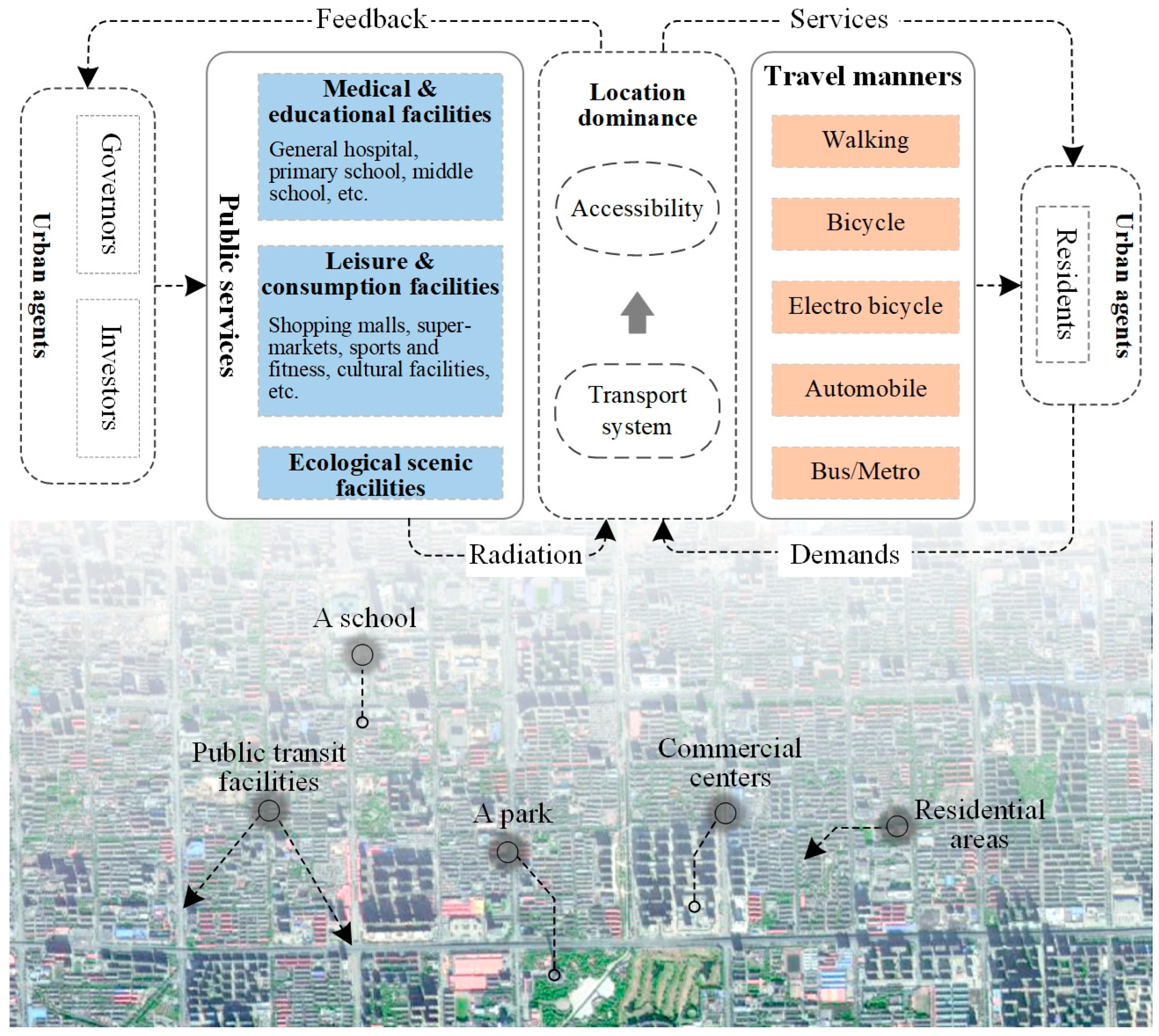
Location dominance, as both a cause and consequence of the interaction between urban agents (i.e., residents, governors, and investors), is developed in this paper as an indicator to evaluate the spatial heterogeneity and equality of public services. There is spatial friction or time costs when residents meet their demands for public services via different transportation options. Correspondingly, the spatial friction from the transportation system also affects the radiation extent of public services. Based on feedback related to location dominance, governors will consider spatial equality in terms of obtaining services, and investors will consider the investment profit from constructing services in different positions. Thus, the spatial heterogeneity of location can help (1) residents choose reasonable transportation, or choose an appropriate residential area; (2) investors calculate the return rate related to the choice of investing location; and (3) governors obtain the basis on which to improve the quality of urban space. The workflow of location dominance is shown in Figure 1.
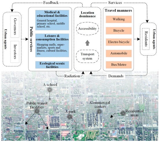
Figure 1.
The workflow of location dominance.
3. Methodology
3.1. Study Area
Shijiazhuang is the capital of Hebei Province, one of the important cities in the Beijing–Tianjin–Hebei Urban Agglomeration. It is located west of the North China Plain and east of Taihang Mountain. In order to alleviate urban problems caused by overconcentration in the central urban area, a multi-center structure within the metropolitan area (i.e., “one river, both sides, three groups”) was proposed in the Shijiazhuang City Master Plan (2011–2020). Specifically, the structure sits across both sides of the Hutuo River, with the central area and industrial area on the south side and the Zhengding Ancient City and Zhengding New District on the north side. Three groups refer to Gaocheng, Luancheng, and Luquan around the central urban area. Thus, the study area includes the central urban area and four suburban areas, covering 107 street/town districts, between 37°46′ and 38°23′ N, and 114°12′ and 114°58′ E, as shown in Figure 2. By the end of 2022, there were 6.24 million permanent residents in the study area, with an urbanization rate of 87.7% and GDP of CNY 468.14 billion, accounting for 70.5% of the total GDP of Shijiazhuang.
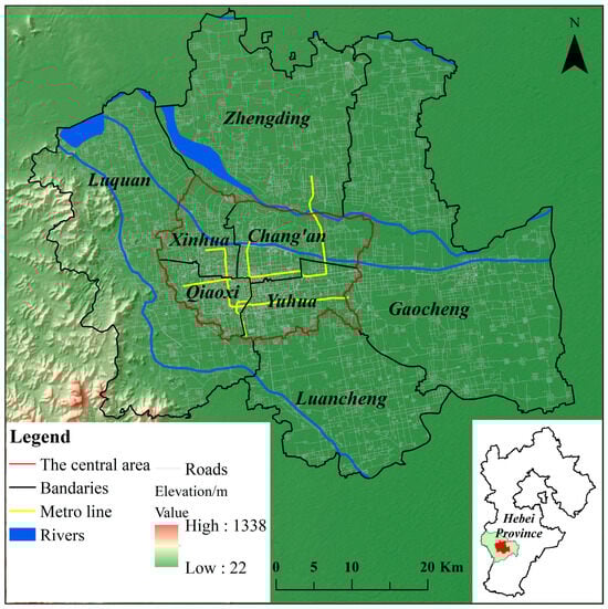
Figure 2.
Shijiazhuang metropolitan area.
3.2. Evaluation System
3.2.1. Public Services
The public services considered in this study are necessary and open access in terms of residents’ daily lives [18,31], including medical and educational facilities, leisure and consumption facilities, and ecological scenic facilities. Leisure and consumption facilities include shopping malls, supermarkets, restaurants, sports and fitness, and cultural facilities. Considering the differences in terms of service levels for the same kinds of facilities in meeting residents’ demands, such as community clinics and general hospitals, we brought forward two screening principles for public services based on Baidu Map classification of the POI data. The principles are as follows: (1) open access for all residents (2) at a certain scale or grade that can service most residents. Finally, we selected 2336 POI related to this study, including 34 types of services. The levels and types of screened services used in this study are provided in Table 1. The details can be seen in the Supplementary Materials.

Table 1.
Levels and types of public services.
3.2.2. Weight Calculation Method
In consideration of the various demands for residents, the combined AHP-entropy method weights of multiple indicators are used to assess the contribution of different service facilities in each location. The analytic hierarchy process (AHP) assigns weights based on the subjective judgments of expert experience with qualitative and quantitative analysis [32]. More specifically, a hierarchal presentation of the decision-making problem is analyzed via a series pairwise comparison judgments to express the relative importance of hierarchy elements [33,34]. While the weights assigned by the entropy method are more objective, and are calculated based on the dispersion of each indicator [35]. The smaller the entropy value of an indicator, the greater its dispersion, and consequently, the more informative and greater its weight [34]. Due to the AHP method relying on subjective judgments and the entropy method ignoring the relevant experience of professionals [36], a composite weight fusing the AHP method and the entropy weight method is used in this paper. In order to make subjective weight and objective weight as close as possible, the minimum relative information entropy weight method (i.e., the Lagrange Multiplier Method) is applied to obtain the composite weights [34]. The expression is as follows:
where is the composite weight of the accessibility of service j. and are the AHP weight and the entropy weight of the accessibility of the service j, respectively.
The process of weight calculation is described in detail in the Supplementary Materials. Weights in terms of the accessibility of public services under different travel modes are shown in Table S2.
3.3. Measuring Accessibility
Accessibility is generally defined as the potential of opportunities for interaction, and is considered one of the main outputs of spatial development [37,38,39]. Accessibility measures comprise the cost of travel and the quality/quantity of opportunities, both of which can be calculated either via location- or person-based ways [36]. Given that residential demand patterns in our study predominantly originate from destination services rather than their points of origin, the location-based radiation model is more suitable for this content. Thus, accessibility can be further defined as the degree to which relevant destinations can be reached given available transport means [31].
The general formulation for accessibility is as follows [38,40]:
where function g reflects the diminishing value of opportunities and competition. refers to the matrix of weighted opportunities. f is an impedance function based on the travel cost to discount the cumulative opportunities. refers to the matrix of the relevant cost elements, e.g., travel time, monetary costs, or externalities (like noise, pollution, congestion).
Compared with other cost elements, travel time is considered as a comprehensive indicator [41], reflecting the influence of urban form and infrastructure. The Network Analysis Tool in ArcGIS 10.6.1 (ESRI China) was used to estimate the radiation extent with a service area analysis. Geographic areas that can be reached from a set of facilities (points) within specified travel time costs (e.g., 5 min, 10 min, 15 min) were generated. The key in terms of network analysis is to create traffic network datasets according to traffic speeds determined by travel modes and alternative road degrees, as shown in Table 2 and Table 3.
Table 2.
Alternative roads for different travel modes.
Table 3.
Traffic speeds with different travel modes and road degrees.
Travel time through a certain route was calculated as follows:
where is the shortest travel time to service s (the unit: minute). represents the length of the fastest route (the unit: km). refers to traffic speed on road d via travel mode m (the unit: km/h), as detailed in Table 3.
A time-weighted cumulative opportunities (also called gravity-based, potential) formulation with a negative power decay function was implied in this study [40]. The formula is as follows:
where is the accessibility of service s via travel mode m; the larger the value, the shorter the travel time, which indicates that it is easier to arrive at the service. Impedance function f assigns lower weights to opportunities with greater time costs compared to less costly alternatives that are reachable from the same location. A constant matrix M is assigned to function g, referring to the spatial distribution of opportunities. A maximum expected travel time of 60 min was set for this study, considered as a “one-hour travel circle”. If is less than 1, the travel time is over 1h; otherwise, the travel time is under 1 h.
3.4. Measuring Location Dominance
Location dominance in a specific location can be quantified by accumulating access opportunities to multiple services. A multi-factor fusion model with a weighted sum rule was used to measure location dominance in each grid, calculated as follows:
where is the location dominance based on travel mode m in grid i. is the accessibility of service s via travel mode m in grid i. The value range of is from 0 to 12. equal to 12 indicates that grid i is within a “5 min access circle” based on travel mode m. of less than 1 means that grid i is beyond the “1 h access circle” of all services based on travel mode m; otherwise, it is within the “1 h access circle”.
3.5. Quantifying the Equality of Location Dominance
Measuring location dominance provides a fine-grained index for assessing the distribution equality of public services across a region. It serves as a proxy to determine whether the distribution of public services among different streets or towns is equitable. To address the need for a comparable index to assess equality, researchers have adopted Lorenz curves and Gini coefficients in a range of urban studies [9,43,44,45]. In this study, Gini coefficients are used to measure the overall level of equity in location dominance of public services at the street/town level. Before calculating the Gini coefficients, we need to draw the Lorenz curves of location dominance for different travel modes, based on their cumulative share and the cumulative share of the total resident population at the street/town level. The total resident population at the street/town level was obtained from the Seventh National Census (2020). The share of the total resident population for each street/town unit was ranked from low to high. We used the cumulative share of the total resident population as the horizontal axis and the corresponding cumulative share of location dominance as the vertical axis to draw the Lorenz curves for different travel modes. The Gini coefficient reflects the ratio of the area between the Lorenz curve and the line of absolute equality [9,46]. The Gini coefficient can be calculated using the following formula [9,44]:
where n is the number of streets/towns in the study area; the value of k, ranking from 1 to n, refers to an order of the street/town unit based on the share of the total resident population from low to high; represents the cumulative share of the total resident population at the kth street/town unit, , ; and represents the cumulative share of location dominance at the kth street/town unit, , . The Gini coefficient can be divided into four levels: absolute equality (0 ≤ Gini < 0.2), equality (0.2 ≤ Gini < 0.3), relative equality (0.3 ≤ Gini < 0.4), and inequality (0.4 ≤ Gini ≤ 1) [9].
4. Results
4.1. Spatial Patterns of Location Dominance
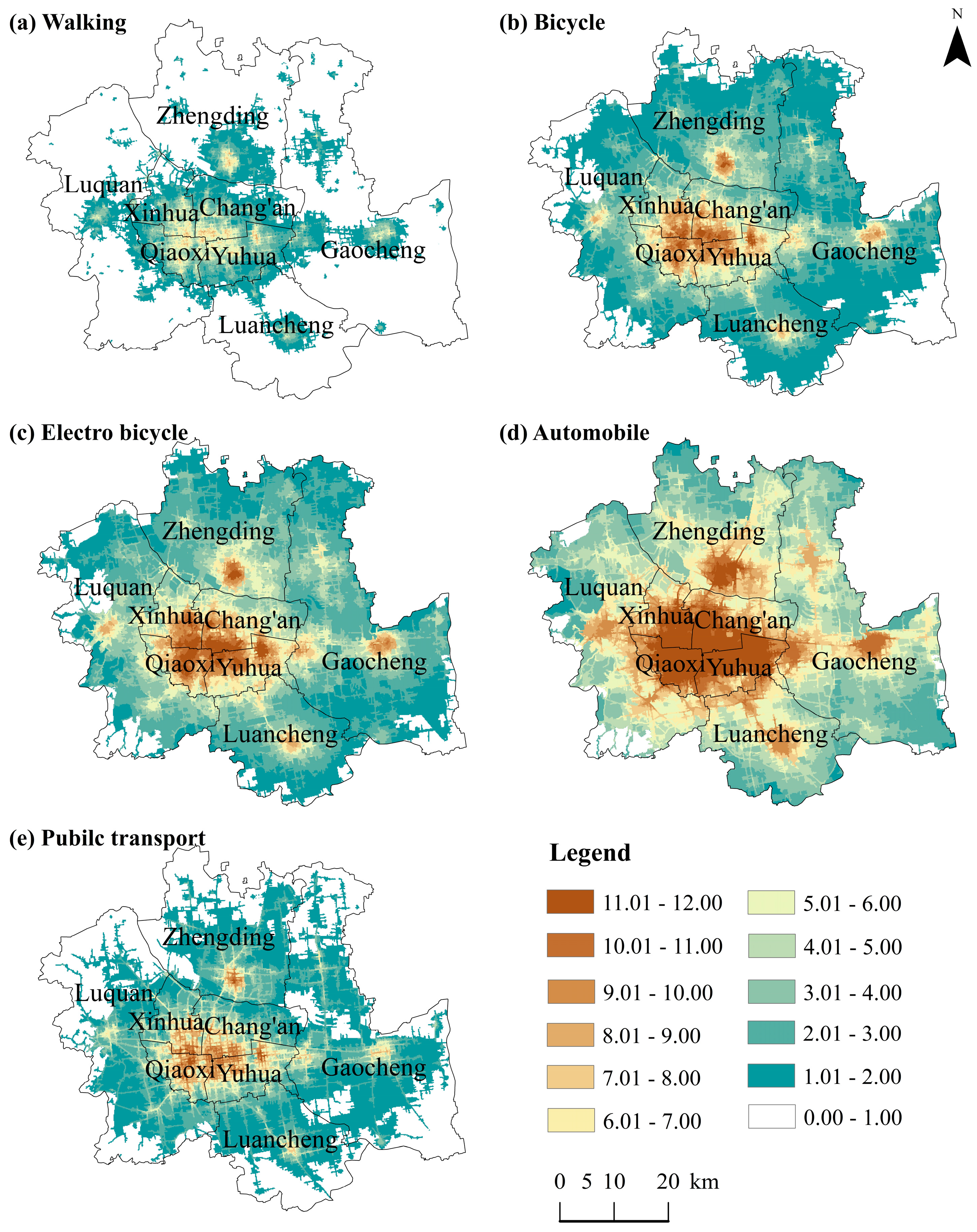
Location dominance in Shijiazhuang followed a strong core–periphery pattern, which is higher in the central urban area and lower in the suburban areas (Figure 3 and Figure 4). There are four sub-core–periphery patterns in the suburban areas, as larger populations and higher economic activity are concentrated in their central streets or towns, while the peripheral areas have smaller populations and lower economic activity.
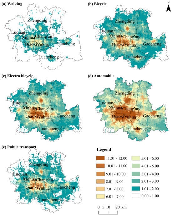
Figure 3.
Spatial patterns of location dominance via alternative travel modes.

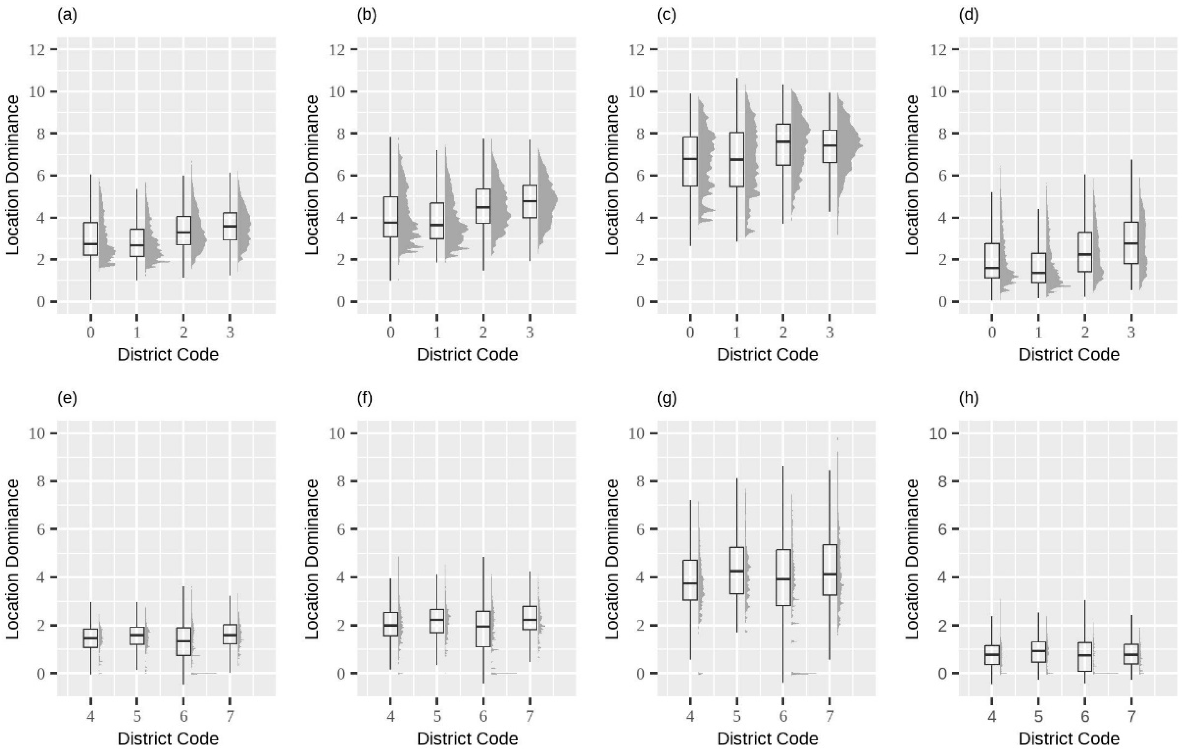
Figure 4.
Differences in location dominance between different travel modes. (a,e) Differences between bicycles and walking. (b,f) Differences between electro bicycles and walking. (c,g) Differences between automobiles and walking. (d,h) Differences between public transport and walking. District codes 0–3 refer to Xinhua, Chang’an, Yuhua, and Qiaoxi, respectively; i.e., the central urban area. District codes 4–7 refer to Gaocheng, Luancheng, Luquan, and Zhengding, respectively; i.e., the four suburban areas.
The core–periphery pattern is significantly different for different travel modes, as indicated in the 100 m × 100 m grid-based maps (see Figure 3). Efficient travel modes can greatly improve location dominance. The coverage ratio for grids with a location dominance greater than 1 is 96.5% via automobile, 90.6% via electro bicycle, 84.4% via bicycle, 65% via public transportation, and less than 30% via walking. Consistently, the relative differences between the location dominance of different travel modes are more telling than the absolute ratio (see Figure 4). Compared with walking, the location dominance of the bicycle is improved by more than two points in the central urban area (i.e., saving more than 10 min) and by about one point in four suburban areas (i.e., saving about 5 min) (Figure 4a,e). The increase in the location dominance of electro bicycles is about four points in the central urban area and about two points in the suburban area (Figure 4b,f). The automobile is the most efficient travel mode, demonstrating the greatest improvement in location dominance, with an increase of more than six points in the central urban area and approximately four points in the suburban area (as shown in Figure 4c,g). By contrast, the location dominance of public transportation shows the least improvement compared to walking, as seen in Figure 4d,h, while it significantly increases along the public bus line (see Figure 3e).
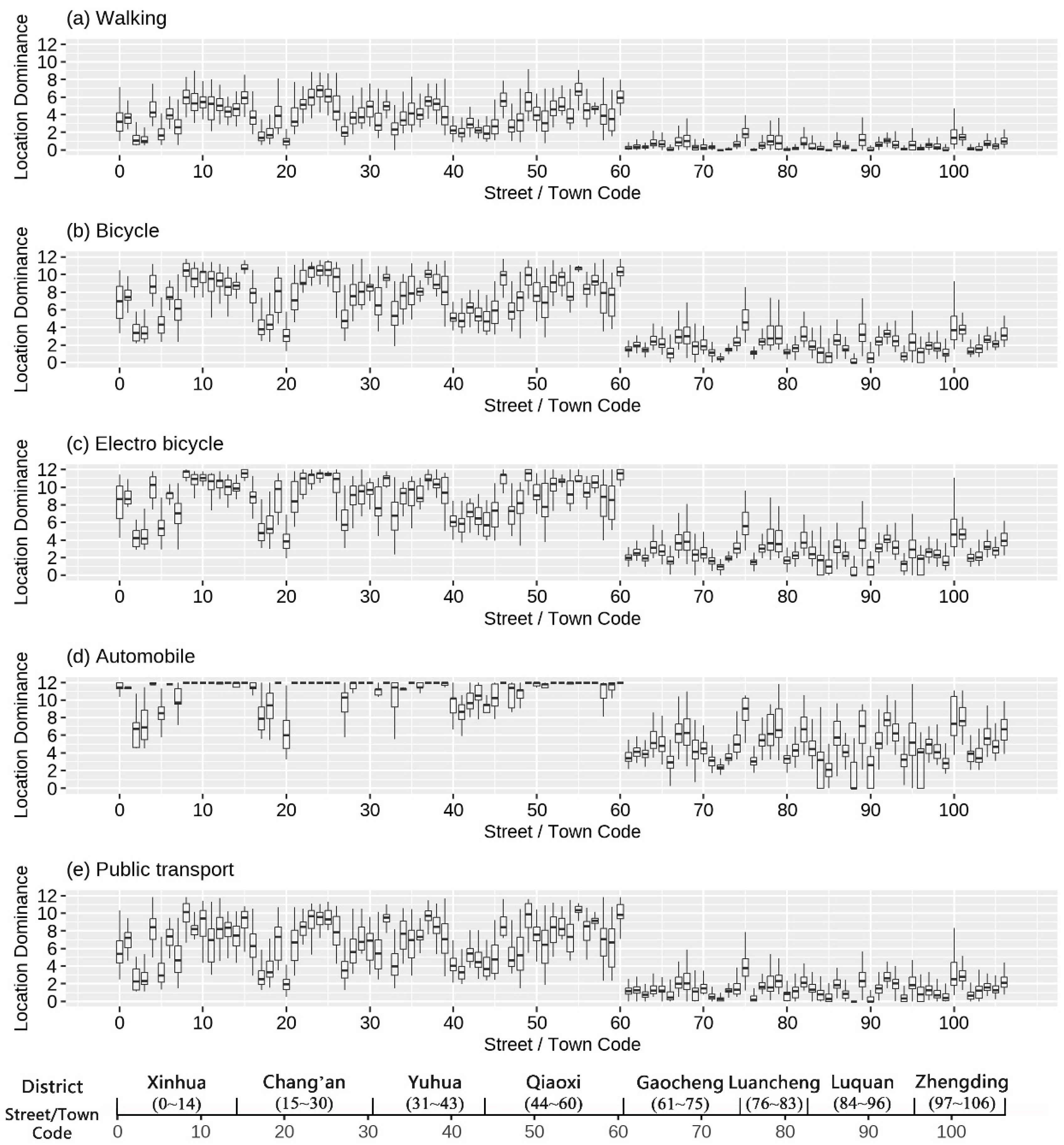
In order to further analyze the distribution of location dominance at the street/town level, boxplots were generated in Figure 5. Location dominance in the central urban area is relatively higher. The number of streets/towns with a location dominance of not less than four (i.e., within a 15 min traffic circle) accounted for 80% of all streets/towns. Furthermore, coverage within the “15 min traffic circle” of public services can reach 12.1% of the metropolitan area. In contrast, location dominance in suburban areas is generally low, but automobile travel can significantly improve it. Specifically, with respect to the automobile travel mode, the number of streets/towns with a location dominance of not less than four accounts for 37% of the total number of streets in the suburban area. With respect to other travel modes, the number of streets with an average location dominance of not less than four (i.e., within a 15 min traffic circle) does not exceed three streets/towns.
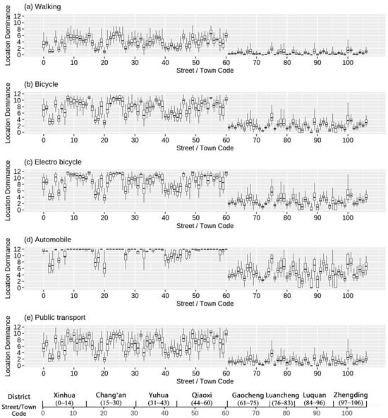
Figure 5.
Boxplots of location dominance at the street/town level.
These equality spatial patterns are not absolute when travel modes are taken into consideration. To quantify the equality of location dominance, the Lorenz curves and the Gini coefficients of different travel modes were calculated based on the cumulation of the share of location dominance and the total resident population at the street/town scale (Figure 6). We found that the Gini coefficients of location dominance by automobile were much lower than for other travel modes. Specifically, the Gini coefficient for automobiles indicated comparative equality (0.2 < Gini < 0.3), while for electric bicycles it was between relative equality (0.3 < Gini < 0.4). The remaining travel modes exhibited inequality, with Gini coefficients exceeding the warning line, i.e., 0.4. These results indicate that efficient vehicles can alleviate spatial inequality.
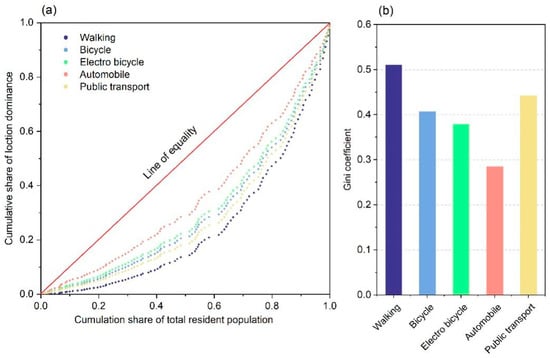
Figure 6.
Lorenz curves and Gini coefficients of location dominance based on 107 streets/towns in Shijiazhuang. The diagram (a) shows Lorenz curves for different travel modes. The red line in (a) represents a case of complete equality. The diagram (b) indicates the Gini coefficients for different travel modes.
4.2. Correlations Between the Results and Urban Development Factors
To evaluate the performance of the proposed method, we calculated the correlations between the results and three key intra-urban development factors, such as nighttime lighting, land use intensity, and population retention rate.
Nighttime light observed from space can serve as a reliable proxy to detect, estimate, and monitor socioeconomic dynamics at a grid scale [47,48]. A nighttime light grid with 100 m × 100 m resolution was obtained from Luojia1-01 Nighttime Light satellite imagery that had undergone radiation correction, standardized stretching, and resampling analysis. Details of these processes are provided in the Supplementary Materials. At the same time, to ensure that the spatial extent of the location dominance results aligned with the nighttime light data, the results were masked to include only areas where nighttime light data were greater than 0. Figure 7 shows scatterplots of the masked results vs. nighttime light data, with each accompanied by its corresponding unary regression line across the five subplots. The p-value for each subplot was less than 0.001, indicating that the linear correlation between the two variables was extremely significant, i.e., not occurring by chance. The adjusted R-squared was employed to gauge the model’s fit to the observed data, effectively mitigating the overfitting issue by accounting for the number of predictors and the sample size. There was a positive correlation between different travel modes and nighttime light intensity. The strength of the linear relationship between the five travel modes and nighttime lighting decreases in the following order: walking has the strongest relationship, followed by public transport, bicycles, electric vehicles, and automobiles (see red lines in the subplots of Figure 7). Similarly, the steepness of the red line in the subplots indicates that the extent of socioeconomic improvement driven by the degree of location dominance follows the same order.
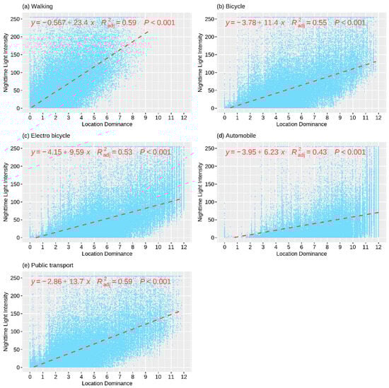
Figure 7.
Scatterplots of the location dominance results vs. nighttime light intensity. The red dashed lines in the five subplots indicate corresponding unary regression lines.
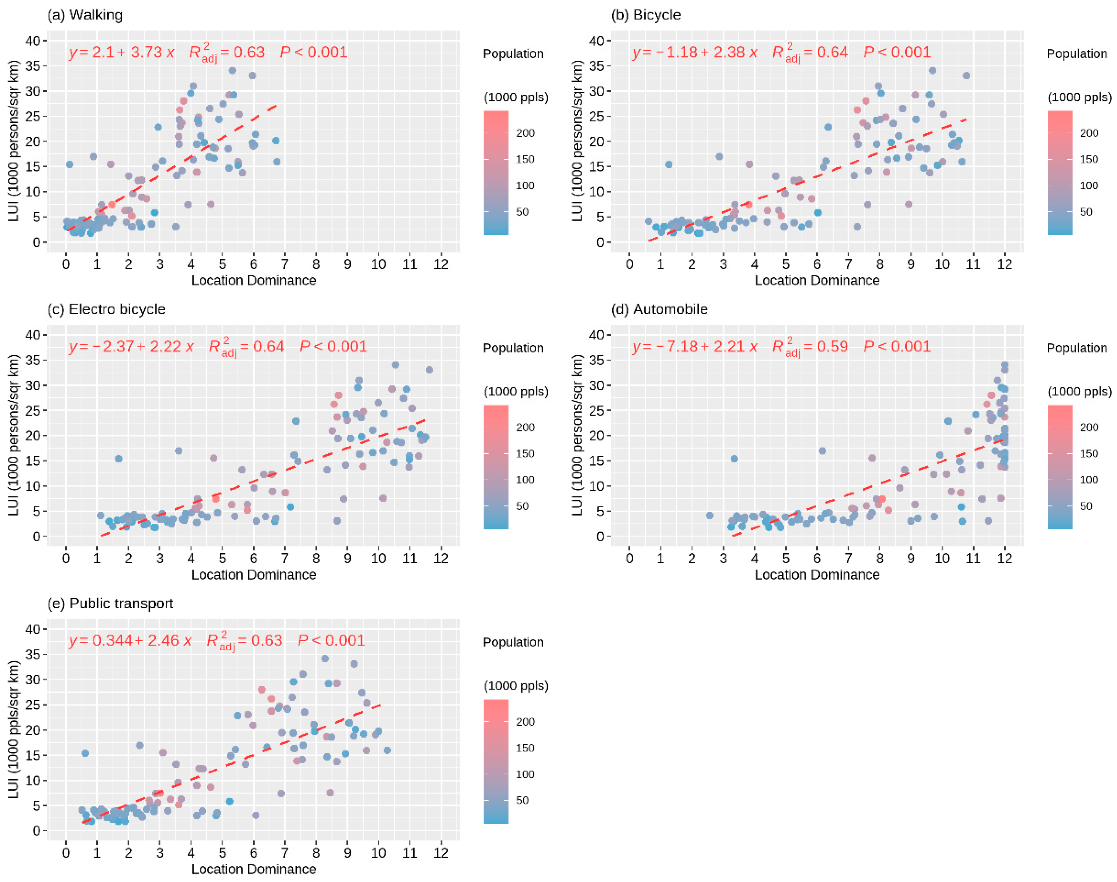
Land use intensity refers to the extent and degree of urban land development, reflecting both the density of human activities and the pressure these activities exert on the land [49,50,51,52]. Following Boserup’s theory, we had considered land use intensity in terms of population and suitable land [53,54], reflecting population pressure on urban land. The correlations between location dominance and land use intensity at the street or town level are shown in the scatterplots (Figure 8). The p-value indicates an extremely significant linear relationship between the two variables (i.e., p-value < 0.001). The adjusted R-squared value is used to assess the explanatory ability of location dominance with respect to land use intensity, ranging from 0.59 to 0.64. There is also a positive correlation between different travel modes and land use intensity. That is to say, regions with high location dominance also tend to have high land use pressures, and vice versa. Both the strength of the explanatory power and the steepness of the red lines (in the subplots of Figure 8) are inversely related to vehicle efficiency, showing a gradual decline from walking to automobiles. Consistently, the impact of increased location dominance on land use intensity is also closely related to vehicle efficiency, following the same pattern.
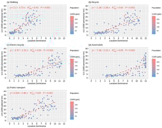
Figure 8.
Scatterplots of location dominance vs. land use intensity. Land use intensity, abbreviated as LUI, is plotted on the y-axis, with the unit being 1000 persons per square kilometer. The red dashed lines in the five subplots indicate corresponding unary regression lines. The gradient color of the points in the scatterplots represents the total current resident population (with the unit being 1000 persons).
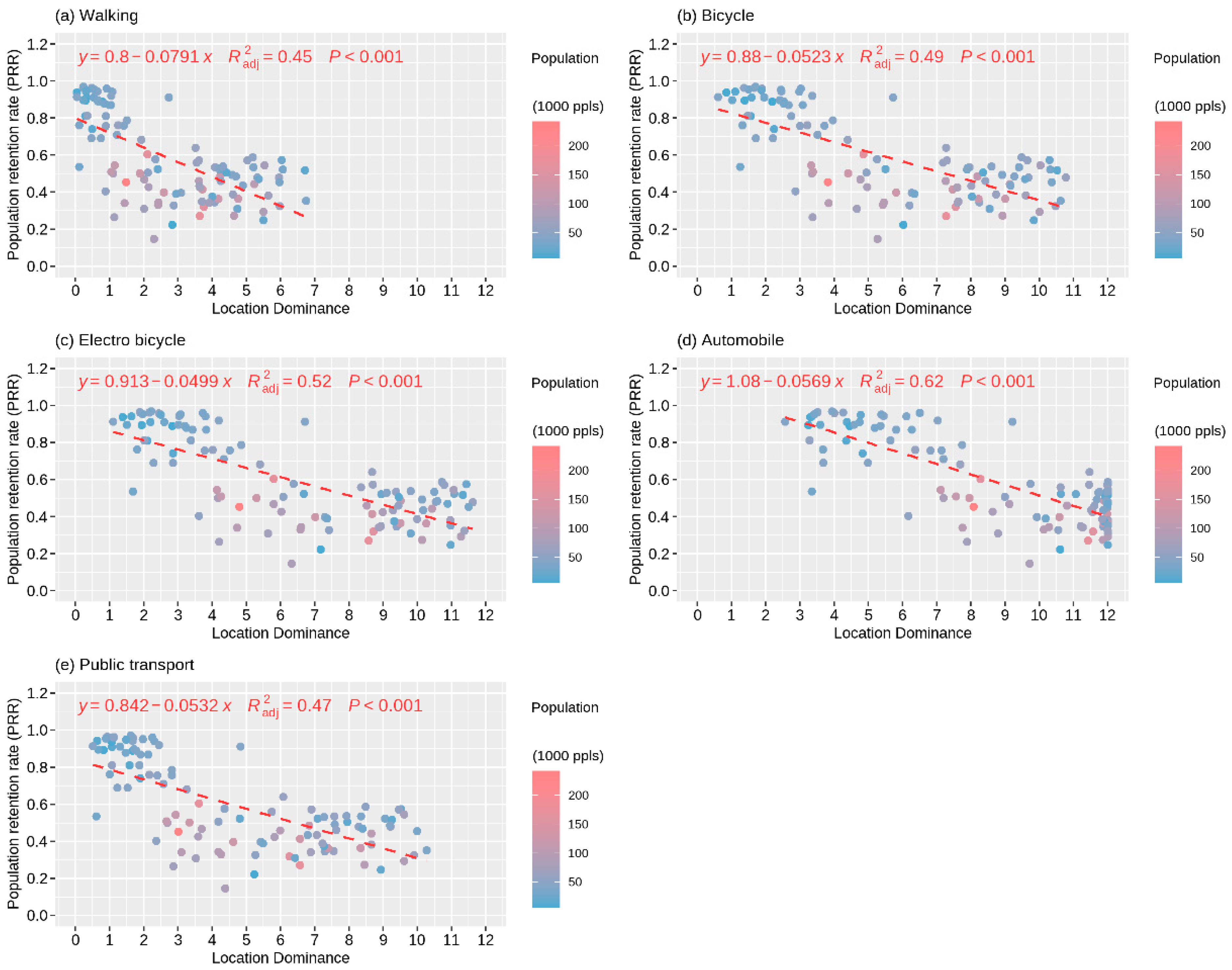
The population retention rate, as defined within China’s hukou registration system [55,56], quantifies the persistence or stability of the registered population and serves as a key measure of population migration. This rate reflects the relationship between hukou-registered place and current residence by calculating the proportion of the original registered population that remains within the total population over a decade. The subplots in Figure 9 demonstrate that the p-value is less than 0.001, indicating an extremely significant linear relationship between location dominance and population retention rate at the street or town level. The explanatory power of these regression models, as indicated by the adjusted R-squared values, ranges from 0.45 to 0.62. The two variables exhibit a negative correlation, suggesting that a decrease in location dominance is associated with an increase in the population retention rate.
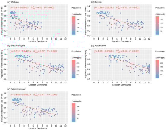
Figure 9.
Scatterplots of location dominance vs. the population retention rate. The red dashed lines in the five subplots indicate corresponding unary regression lines. The gradient color of the points in the scatterplots represents the total current resident population (with the unit being 1000 persons).
5. Discussion and Conclusions
5.1. Spatial Disparities in Public Service Accessibility in Shijiazhuang
The inevitability of a disparity in public service distribution is recognized [5,44,57]. The results show that the accessibility of public services in Shijiazhuang exhibits a strong core–periphery pattern, similar to the patterns evidenced by studies in various cities [31]. Efficient travel modes can greatly enhance location dominance [44], with bicycles, electric bicycles, and automobiles showing an increase of between two points and four points in the central urban area and an increase of between one point and four points in the four suburban areas compared to walking. This result is confirmed by comprehensive traffic survey data from Shijiazhuang collected in 2007 and 2015. The proportion of residents choosing private cars, electric bicycles, and public transport increased by 13.0%, 11.8%, and 8.0%, respectively, from 2007 to 2015 [58]. The proportion of residents choosing walking remained stable, while the proportion choosing to use bicycles fell by 29.1% during the same period. Although bicycles are promoted as a sustainable mobility solution, they tend to be constrained by high costs associated with travel distance through the road network [59]. Although bike-sharing services are globally prevalent, their accessibility may be conditioned by some spatial constraints, mainly due to restrictions on the service’s operational area [60]. Consistently, Li et al. (2020) [61] found that almost 90% of bicycle trips are less than 30 min or 5 km, based on a massive dockless bike-sharing dataset for Shanghai. Electric bicycles with a maximum speed of 25 km/h are rapidly increasing across the world [62]. Electric bicycles address the issue of longer travel time compared to traditional bicycles, which have lower speeds. Nevertheless, their safety issues, especially those concerning crashes [62], cannot be overlooked.
In practice, although Shijiazhuang has implemented various public transport policies, such as free transport for special groups, “green travel days”, and free transport on “vehicle-restricted days”, public transport still has the least impact on location dominance. Most residents prefer using private, efficient, and mobile vehicles, such as private cars, electric bicycles, and bicycles, which accounted for 38.6% of the total in 2015, rather than public transport, which accounted for 15.2% in 2015. This preference can effectively improve the accessibility of public services and alleviate inequality in their distribution. This trend is impacted by at least three factors: (1) People’s travel habits are gradually changing with the renewal of transportation tools. (2) The public transportation system relies on existing infrastructure, which has a relatively slow renewal rate and is losing alignment with rapidly evolving residential and commercial facilities. (3) The walking distance from the origin or destination to the public bus station, referred to as the first/last kilometer, leads people to abandon public transport. Similar situations are observed in many cities across countries [63,64,65]. These findings offer crucial guidance for policymakers and urban designers in their efforts to enhance urban equality and sustainability.
5.2. Validation of Location Dominance for Public Service Accessibility Assessment
Spatial heterogeneity or disparity within cities arises not from a single factor, but from the interplay of various elements in urban development. Understanding the relationships between three key developing elements (i.e., nighttime lighting data, land use intensity, and population retention rate) and location dominance is crucial for assessing both the impacts and the rationality of our results. There is an extremely significant linear correlation between these three elements and location dominance. This correlation positively impacts the first two factors and negatively affects the last one. Therefore, nighttime lighting can also serve as an indicator in terms of addressing urban infrastructure inequality [5], and land use intensity is a general indicator widely used in urban studies [52]. Thus, this linear relationship demonstrates the rationality of the results. It is noteworthy that there is no correlation between location dominance and population quantitative indicators, such as total population, hukou-registered population, and aging population, yet there is a significant correlation with the population retention rate at the town/street level. This means that location dominance has a direct impact on the separation rate between current residence and hukou-registered place, rather than just an absolute number of the population. Our finding suggests that location dominance can address the question of the population migration ratio (a relative variable), rather than the question of which population it serves.
5.3. Characteristics of the Method in Terms of Granularity, Universality and Practicability
This study expresses the spatial characteristics of public service accessibility in a continuous numerical form, based on a combination of transportation network analysis and multi-factor fusion models. Compared to the buffer zone analysis and kernel density estimation methods used in current urban planning, these results are more refined and reliable at a smaller granularity. Travel time measurement inherently reflects the constraints imposed by urban morphology and transportation infrastructure, and it serves as the most robust distance–decay indicator for accessibility modeling. This universality ensures the methodological transferability of our framework across diverse urban contexts. Recent advancements in geospatial APIs, such as Amap’s Route Planning Service v2.0, significantly enhance temporal accuracy by incorporating real-world routing nuances through the simulation of actual navigation scenarios. In addition, due to the strong spatial correlation inherent in daily commutes, which is not considered in the evaluation process, this study focuses on non-commute trips, such as those for shopping, entertainment, or healthcare. Comprehensive traffic survey data show that the proportion of non-commute trips increased slightly between 2007 and 2015, accounting for 34.9% by 2015 [58]. Future research should consider both non-commute trips and commute trips to enhance the evaluation system of location dominance, such as utilizing mobile phone cellular network data and residents’ travel patterns [66,67]. This study offers a framework to tackle urban issues within the realms of urban diagnostics and urban renewal. Compared to comprehensive traffic survey data, this framework can not only quickly diagnose the spatial distribution of accessibility for different travel modes but also subtly identify spatial accessibility equality in terms of public services.
The concept of location dominance provides a proxy to comprehensively evaluate the spatial equality of public services in a certain region based on accessibility. In contrast, an increasing amount of attention is being paid to the “15 min city”, an idea that emphasizes proximity-based planning, focusing on living locally and de-mobility [65,68]. Specifically, the core essence of this idea is to reduce unnecessary travel so that residents’ daily activities can be accommodated within a 15 min walking radius [65]. Although the “15 min city” concept has the potential to bring a paradigm change to the future of urban and transportation planning, it is crucial to take a long-term perspective on its implementation principles and assess comprehensively whether cities meet the requirements of the concept [69]. Most services, like food retailers, have a spatial hierarchical structure, and their distribution and service extent follow the “Pareto Principle”. For example, upper-level food retailers accounted for only 6.9 percent of total retailers but contributed to 96.3 percent of total accessibility [70]. Thus, if a hierarchical accessibility framework can be constructed that integrates the location dominance of services at various levels within local and regional contexts, it can effectively promote livability, equity, and sustainability in urban planning [68,71].
Supplementary Materials
The following supporting information can be downloaded at: https://www.mdpi.com/article/10.3390/land14040830/s1, Figure S1. non-motorized road, motor way and public transport network and the location of urban services. (a) refers to the non-motorized road network, which includes Trunk ways, Primary Roads, Secondary Roads, Tertiary Roads, and others, for use by walking, bicycles, and electric bicycles. (b) refers the motor way network including Expressway, Trunk Road, Primary Road, Secondary Road, and Tertiary Road. (c) refers public transport network including public bus lines and metro lines. (d) refers different types of urban services; Figure S2. The processed nighttime light image in Shijiazhuang; Figure S3. Geographical distribution of land use intensity at the street or town level; Figure S4. Geographical distribution of population retention rate at the street or town level; Figure S5. Comparison of location dominance in four streets/towns; Table S1. Statistics of urban services; Table S2. Weights of the accessibility for urban services under different travel modes [72,73,74,75].
Author Contributions
Conceptualization, Y.W. and P.P.; methodology, Y.W. and P.P.; software, Y.W.; visualization, P.P. validation, Y.W. and L.P.; formal analysis, Y.W.; writing—original draft preparation, Y.W.; writing—review and editing, Y.W., P.P. and L.P. All authors have read and agreed to the published version of the manuscript.
Funding
This research was financially supported by the National Natural Science Foundation of China (Grant No. 42201278 and 42471336), Major Projects for Humanities and Social Science Research in Hebei Province Universities (Grant No. 2022HY11), and Hebei Normal University Doctoral (Postdoctoral) Research Initiation Project (Grant No. L2024B32).
Data Availability Statement
The original contributions presented in the study are included in the article/Supplementary materials, further inquiries can be directed to the corresponding author.
Conflicts of Interest
The authors declare that they have no known competing financial interests or personal relationships that could have appeared to influence the work reported in this paper.
References
- Elmqvist, T.; Bai, X.; Frantzeskaki, N.; Griffith, C.; Maddox, D.; McPhearson, T.; Parnell, S.; Romero-Lankao, P.; Simon, D.; Watkins, M. Urban Planet: Knowledge Towards Sustainable Cities; Cambridge University Press: Cambridge, UK, 2018. [Google Scholar]
- Department of Economic and Social Affairs, Population Division, Population Division. World Urbanization Prospects: The 2018 Revision. Available online: https://population.un.org/wup (accessed on 5 January 2025).
- Huang, K.; Li, X.; Liu, X.; Seto, K.C. Projecting global urban land expansion and heat island intensification through 2050. Environ. Res. Lett. 2019, 14, 114037. [Google Scholar] [CrossRef]
- Sampson, R.J. Urban sustainability in an age of enduring inequalities: Advancing theory and ecometrics for the 21st-century city. Proc. Natl. Acad. Sci. USA 2017, 114, 8957–8962. [Google Scholar] [CrossRef] [PubMed]
- Pandey, B.; Brelsford, C.; Seto, K.C. Infrastructure inequality is a characteristic of urbanization. Proc. Natl. Acad. Sci. USA 2022, 119, e2119890119. [Google Scholar] [CrossRef] [PubMed]
- Liu, R.; Chen, Y.; Wu, J.; Xu, T.; Gao, L.; Zhao, X. Mapping spatial accessibility of public transportation network in an urban area–A case study of Shanghai Hongqiao Transportation Hub. Transp. Res. Part D Transp. Environ. 2018, 59, 478–495. [Google Scholar] [CrossRef]
- United Nations. Transforming Our World: The 2030 Agenda for Sustainable Development. 2015. Available online: https://sdgs.un.org/2030agenda (accessed on 5 January 2025).
- Wu, F.; Zhang, F. Rethinking China’s urban governance: The role of the state in neighbourhoods, cities and regions. Prog. Hum. Geogr. 2022, 46, 775–797. [Google Scholar] [CrossRef]
- Xu, R.; Yue, W.; Wei, F.; Yang, G.; Chen, Y.; Pan, K. Inequality of public facilities between urban and rural areas and its driving factors in ten cities of China. Sci. Rep. 2022, 12, 13244. [Google Scholar] [CrossRef]
- Zhang, W.; Zhang, X.; Wu, G. The network governance of urban renewal: A comparative analysis of two cities in China. Land Use Policy 2021, 106, 105448. [Google Scholar] [CrossRef]
- Li, X.; Hui, E.C.; Chen, T.; Lang, W.; Guo, Y. From Habitat III to the new urbanization agenda in China: Seeing through the practices of the “three old renewals” in Guangzhou. Land Use Policy 2019, 81, 513–522. [Google Scholar] [CrossRef]
- Guangdong Province Old Town Old Factory Old Village Recreation Association; Policy and Legal Professional Committee of Guangdong Province Old Town Old Factory Building and Old Village Recreation Association; Guangdong Huaxian Runke Law Firm, Lvfang Lvdi Institute. Guangdong Province “Three Old Renewal” (Urban Renewal) Policy Compilation (2022 Edition); Guangdong Province Old Town Old Factory Old Village Recreation Association: Guangzhou, China, 2022. [Google Scholar]
- Xi, J. Hold high the great banner of socialism with Chinese characteristics and strive in unity to build a modern socialist country in all respects. In Proceedings of the 20th National Congress of the Communist Party of China, Beijing, China, 16 October 2022. [Google Scholar]
- Cervero, R.; Murphy, S.; Ferrell, C.; Goguts, N.; Tsai, Y.H.; Arrington, G.B.; Boroski, J.; Smith-Heimer, J.; Golem, R.; Peninger, P.; et al. Transit-Oriented Development in the United States: Experiences, Challenges, and Prospects; Transportation Research Board: Washington, DC, USA, 2004. [Google Scholar]
- Yu, Z.; Zhu, X.; Liu, X. Characterizing metro stations via urban function: Thematic evidence from transit-oriented development (TOD) in Hong Kong. J. Transp. Geogr. 2022, 99, 103299. [Google Scholar] [CrossRef]
- Curtis, C.; Scheurer, J. Planning for sustainable accessibility: Developing tools to aid discussion and decision-making. Prog. Plan. 2010, 74, 53–106. [Google Scholar] [CrossRef]
- Lang, W.; Hui, E.C.; Chen, T.; Li, X. Understanding livable dense urban form for social activities in transit-oriented development through human-scale measurements. Habitat Int. 2020, 104, 102238. [Google Scholar] [CrossRef]
- Verachtert, E.; Mayeres, I.; Vermeiren, K.; Van der Meulen, M.; Vanhulsel, M.; Vanderstraeten, G.; Loris, I.; Mertens, G.; Engelen, G.; Poelmans, L. Mapping regional accessibility of public transport and services in support of spatial planning: A case study in Flanders. Land Use Policy 2023, 133, 106873. [Google Scholar] [CrossRef]
- Zeng, C.; Song, Y.; Cai, D.; Hu, P.; Cui, H.; Yang, J.; Zhang, H. Exploration on the spatial spillover effect of infrastructure network on urbanization: A case study in Wuhan urban agglomeration. Sustain. Cities Soc. 2019, 47, 101476. [Google Scholar] [CrossRef]
- Vale, D.S.; Viana, C.M.; Pereira, M. The extended node-place model at the local scale: Evaluating the integration of land use and transport for Lisbon’s subway network. J. Transp. Geogr. 2018, 69, 282–293. [Google Scholar] [CrossRef]
- Xu, W.; Yang, L. Evaluating the urban land use plan with transit accessibility. Sustain. Cities Soc. 2019, 45, 474–485. [Google Scholar] [CrossRef]
- Ramirez, J. Residential Location Theories and Planning: A General Analysis with Special Reference to Latin America. Master’s Thesis, University of Glasgow, Scotland, UK, 1976. [Google Scholar]
- Bathelt, H.; Glückler, J. Toward a relational economic geography. In Economy: Critical Essays in Human Geography; Routledge: London, UK, 2008. [Google Scholar]
- Dunning, J.H.; Lundan, S.M. Multinational Enterprises and the Global Economy, 2nd ed.; Edward Elgar: Cheltenham, UK; Northampton, MA, USA, 2008. [Google Scholar]
- Kalfadellis, P. Location advantages and repeat investment in Australia: A two-state comparison. Reg. Stud. 2015, 49, 1140–1159. [Google Scholar] [CrossRef]
- Cuervo-Cazurra, Á.; de Holan, P.M.; Sanz, L. Location advantage: Emergent and guided co-evolutions. J. Bus. Res. 2014, 67, 508–515. [Google Scholar] [CrossRef]
- Yang, Y.; Mao, Z. Location advantages of lodging properties: A comparison between hotels and Airbnb units in an urban environment. Ann. Tour. Res. 2020, 81, 102861. [Google Scholar] [CrossRef]
- le Duc, N.; Gammeltoft, P. The role of R&D resource commitment in accessing co-location advantages. J. Int. Manag. 2023, 29, 101015. [Google Scholar] [CrossRef]
- Jin, F.; Wang, C.; Li, X.; Wang, J. China’s regional transport dominance: Density, proximity, and accessibility. J. Geogr. Sci. 2010, 20, 295–309. [Google Scholar] [CrossRef]
- Wang, Z.; Fan, H.; Wang, D.; Xing, T.; Wang, D.; Guo, Q.; Xiu, L. Spatial pattern of highway transport dominance in Qinghai-Tibet Plateau at the county scale. ISPRS Int. J. Geo. Inf. 2021, 10, 304. [Google Scholar] [CrossRef]
- Kompil, M.; Jacobs-Crisioni, C.; Dijkstra, L.; Lavalle, C. Mapping accessibility to generic services in Europe: A market-potential based approach. Sustain. Cities Soc. 2019, 47, 101372. [Google Scholar] [CrossRef]
- Basak, I.; Saaty, T. Group decision making using the analytic hierarchy process. Math. Comput. Model. 1993, 17, 101–109. [Google Scholar] [CrossRef]
- Saaty, T.L. A scaling method for priorities in hierarchical structures. J. Math. Psychol. 1977, 15, 234–281. [Google Scholar] [CrossRef]
- Al-Aomar, R. A combined ahp-entropy method for deriving subjective and objective criteria weights. Int. J. Ind. Eng. 2010, 17, 12–24. [Google Scholar]
- Shannon, C.E. A mathematical theory of communication. Bell Syst. Tech. J. 1948, 27, 379–423. [Google Scholar] [CrossRef]
- Xu, S.; Xu, D.; Liu, L. Construction of regional informatization ecological environment based on the entropy weight modified AHP hierarchy model. Sustain. Comput. Inform. Syst. 2019, 22, 26–31. [Google Scholar] [CrossRef]
- Hansen, W.G. How accessibility shapes land use. J. Am. Inst. Plan. 1959, 25, 73–76. [Google Scholar] [CrossRef]
- Páez, A.; Scott, D.M.; Morency, C. Measuring accessibility: Positive and normative implementations of various accessibility indicators. J. Transp. Geogr. 2012, 25, 141–153. [Google Scholar] [CrossRef]
- Handy, S. Is accessibility an idea whose time has finally come? Transp. Res. Part D Transp. Environ. 2020, 83, 102319. [Google Scholar] [CrossRef]
- Levinson, D.; Wu, H. Towards a general theory of access. J. Transp. Land Use 2020, 13, 129–158. [Google Scholar] [CrossRef]
- Chen, Z.; Li, Y.; Wang, P. Transportation accessibility and regional growth in the Greater Bay Area of China. Transp. Res. Part D Transp. Environ. 2020, 86, 102453. [Google Scholar] [CrossRef]
- CJJ 37-2012; Code for Design of Urban Road Engineering. MOHURD: Beijing, China, 2012.
- Delbosc, A.; Currie, G. Using Lorenz curves to assess public transport equity. J. Transp. Geogr. 2011, 19, 1252–1259. [Google Scholar] [CrossRef]
- Tahmasbi, B.; Mansourianfar, M.H.; Haghshenas, H.; Kim, I. Multimodal accessibility-based equity assessment of urban public facilities distribution. Sustain. Cities Soc. 2019, 49, 101633. [Google Scholar] [CrossRef]
- Martin, A.J.F.; Conway, T.M. Using the Gini Index to quantify urban green inequality: A systematic review and recommended reporting standards. Landsc. Urban Plan. 2025, 254, 105231. [Google Scholar] [CrossRef]
- Shirmohammadli, A.; Louen, C.; Vallée, D. Exploring mobility equity in a society undergoing changes in travel behavior: A case study of Aachen, Germany. Transp. Policy 2016, 46, 32–39. [Google Scholar] [CrossRef]
- Bennett, M.M.; Smith, L.C. Advances in using multitemporal night-time lights satellite imagery to detect, estimate, and monitor socioeconomic dynamics. Remote Sens. Environ. 2017, 192, 176–197. [Google Scholar] [CrossRef]
- Levin, N.; Kyba, C.C.; Zhang, Q.; de Miguel, A.S.; Román, M.O.; Li, X.; Portnov, B.A.; Molthan, A.L.; Jechow, A.; Miller, S.D.; et al. Remote sensing of night lights: A review and an outlook for the future. Remote Sens. Environ. 2020, 237, 111443. [Google Scholar] [CrossRef]
- Erb, K.H. How a socio-ecological metabolism approach can help to advance our understanding of changes in land-use intensity. Ecol. Econ. 2012, 76, 8–14. [Google Scholar] [CrossRef]
- Wellmann, T.; Haase, D.; Knapp, S.; Salbach, C.; Selsam, P.; Lausch, A. Urban land use intensity assessment: The potential of spatio-temporal spectral traits with remote sensing. Ecol. Indic. 2018, 85, 190–203. [Google Scholar] [CrossRef]
- Xia, C.; Yeh, A.G.O.; Zhang, A. Analyzing spatial relationships between urban land use intensity and urban vitality at street block level: A case study of five Chinese megacities. Landsc. Urban Plan. 2020, 193, 103669. [Google Scholar] [CrossRef]
- Xu, F.; Wang, Z.; Chi, G.; Zhang, Z. The impacts of population and agglomeration development on land use intensity: New evidence behind urbanization in China. Land Use Policy 2020, 95, 104639. [Google Scholar] [CrossRef]
- Ellis, E.C.; Ramankutty, N. Putting people in the map: Anthropogenic biomes of the world. Front. Ecol. Environ. 2008, 6, 439–447. [Google Scholar] [CrossRef]
- Erb, K.H.; Fetzel, T.; Haberl, H.; Kastner, T.; Kroisleitner, C.; Lauk, C.; Niedertscheider, M.; Plutzar, C. Beyond inputs and outputs: Opening the black-box of land-use intensity. In Social Ecology: Society-Nature Relations Across Time and Space; Springer Nature: Cham, Switzerland, 2016; pp. 93–124. [Google Scholar] [CrossRef]
- Chan, K.W.; Zhang, L. The hukou system and rural-urban migration in China: Processes and changes. China Q. 1999, 160, 818–855. [Google Scholar] [CrossRef]
- Qi, W.; Abel, G.J.; Liu, S. Geographic transformation of China’s internal population migration from 1995 to 2015: Insights from the migration centerline. Appl. Geogr. 2021, 135, 102564. [Google Scholar] [CrossRef]
- Nicoletti, L.; Sirenko, M.; Verma, T. Disadvantaged communities have lower access to urban infrastructure. Environ. Plan. B Urban Anal. City Sci. 2023, 50, 831–849. [Google Scholar] [CrossRef]
- Fu, L. A strategic plan and current situation analysis of public transit in Shijiazhuang City. Qinghai Transp. Sci. Technol. 2018, 10–18. [Google Scholar]
- Rosas-Satizábal, D.; Guzman, L.A.; Oviedo, D. Cycling diversity, accessibility, and equality: An analysis of cycling commuting in Bogotá. Transp. Res. Part D Transp. Environ. 2020, 88, 102562. [Google Scholar] [CrossRef]
- Giuffrida, N.; Pilla, F.; Carroll, P. The social sustainability of cycling: Assessing equity in the accessibility of bike-sharing services. J. Transp. Geogr. 2023, 106, 103490. [Google Scholar] [CrossRef]
- Li, A.; Huang, Y.; Axhausen, K.W. An approach to imputing destination activities for inclusion in measures of bicycle accessibility. J. Transp. Geogr. 2020, 82, 102566. [Google Scholar] [CrossRef]
- Schepers, J.P.; Fishman, E.; den Hertog, P.; Wolt, K.K.; Schwab, A.L. The safety of electrically assisted bicycles compared to classic bicycles. Accid. Anal. Prev. 2014, 73, 174–180. [Google Scholar] [CrossRef] [PubMed]
- Tjahjono, T.; Kusuma, A.; Septiawan, A. The greater Jakarta area commuters travelling pattern. Transp. Res. Procedia 2020, 47, 585–592. [Google Scholar] [CrossRef]
- Ayuriany, T.; Lee, J.; Hidayati, I. What access-for-all entails? Examining commuting experiences from subjective and objective accessibility in a fast-growing city, Jakarta. Asian Transp. Stud. 2023, 9, 100115. [Google Scholar] [CrossRef]
- Jin, T.; Wang, K.; Xin, Y.; Shi, J.; Hong, Y.; Witlox, F. Is a 15-minute city within reach? measuring multimodal accessibility and carbon footprint in 12 major american cities. Land Use Policy 2024, 142, 107180. [Google Scholar] [CrossRef]
- Chin, K.; Huang, H.; Horn, C.; Kasanicky, I.; Weibel, R. Inferring fine-grained transport modes from mobile phone cellular signaling data. Comput. Environ. Urban Syst. 2019, 77, 101348. [Google Scholar] [CrossRef]
- Hadachi, A.; Pourmoradnasseri, M.; Khoshkhah, K. Unveiling large-scale commuting patterns based on mobile phone cellular network data. J. Transp. Geogr. 2020, 89, 102871. [Google Scholar] [CrossRef]
- Mouratidis, K. Time to challenge the 15-minute city: Seven pitfalls for sustainability, equity, livability, and spatial analysis. Cities 2024, 153, 105274. [Google Scholar] [CrossRef]
- Papadopoulos, E.; Sdoukopoulos, A.; Politis, I. Measuring compliance with the 15-minute city concept: State-of-the-art, major components and further requirements. Sustain. Cities Soc. 2023, 99, 104875. [Google Scholar] [CrossRef]
- Chen, B.Y.; Fu, C.; Wang, D.; Jia, T.; Gong, J. How Retailer hierarchy shapes food accessibility: A case study using machine learning method to delineate service areas and hierarchical levels of food retailers. Ann. Assoc. Am. Geogr. 2024, 114, 611–632. [Google Scholar] [CrossRef]
- Bruno, M.; Melo, H.P.M.; Campanelli, B.; Loreto, V. A universal framework for inclusive 15-minute cities. Nat. Cities 2024, 1, 633–641. [Google Scholar] [CrossRef]
- Elvidge, C.D.; Ghosh, T.; Hsu, F.-C.; Zhizhin, M.; Bazilian, M. The Dimming of Lights in China during the COVID-19 Pandemic. Remote Sens. 2020, 12, 2851. [Google Scholar] [CrossRef]
- Jiang, W.; He, G.; Long, T.; Guo, H.; Yin, R.; Leng, W.; Liu, H.; Wang, G. Potentiality of Using Luojia 1-01 Nighttime Light Imagery to Investigate Artificial Light Pollution. Sensors 2018, 18, 2900. [Google Scholar] [CrossRef] [PubMed]
- Shi, K.; Chang, Z.; Chen, Z.; Wu, J.; Yu, B. Identifying and evaluating poverty using multisource remote sensing and point of interest (POI) data: A case study of Chongqing, China. J. Clean. Prod. 2020, 255, 120245. [Google Scholar] [CrossRef]
- Zhou, Y.; Smith, S.J.; Elvidge, C.D.; Zhao, K.; Thomson, A.; Imhoff, M. A cluster-based method to map urban area from DMSP/OLS nightlights. Remote Sens. Environ. 2014, 147, 173–185. [Google Scholar] [CrossRef]


Disclaimer/Publisher’s Note: The statements, opinions and data contained in all publications are solely those of the individual author(s) and contributor(s) and not of MDPI and/or the editor(s). MDPI and/or the editor(s) disclaim responsibility for any injury to people or property resulting from any ideas, methods, instructions or products referred to in the content. |
© 2025 by the authors. Licensee MDPI, Basel, Switzerland. This article is an open access article distributed under the terms and conditions of the Creative Commons Attribution (CC BY) license (https://creativecommons.org/licenses/by/4.0/).