Identification of Key Drivers of Land Surface Temperature Within the Local Climate Zone Framework

Abstract

The surface urban heat island (SUHI) effect, driven by human activities and land cover changes, leads to elevated temperatures in urban areas, posing challenges to sustainability, public health, and environmental quality. While SUHI drivers at large scales are well-studied, finer-scale thermal variations remain underexplored. This study employed the Local Climate Zones (LCZs) framework to analyze land surface temperature (LST) dynamics in Zhengzhou, China. Using 2022 mean LST data derived from a single-channel algorithm, combined with field surveys and remote sensing techniques, we examined 30 potential driving factors spanning natural and anthropogenic conditions. Results show that built-type LCZs had higher average LSTs (31.10 °C) compared with non-built LCZs (28.91 °C), with non-built LCZs showing greater variability (10.48 °C vs. 6.76 °C). Among five major driving factor categories, landscape pattern indices dominated built-type LCZs, accounting for 44.5% of LST variation, while Tasseled Cap Transformation indices, particularly brightness, drove 42.8% of the variation in non-built-type LCZs. Partial dependence analysis revealed that wetness and landscape fragmentation reduce LST in built-type LCZs, whereas GDP, imperviousness, and landscape cohesion increase it. In non-built LCZs, population density, connectivity, and brightness raise LST, while wetness and atmospheric dryness provide cooling effects. These findings highlight the need for LCZ-specific SUHI mitigation strategies. Built-type LCZs require urban form optimization, enhanced landscape connectivity, and expanded green infrastructure to reduce heat accumulation. Non-built LCZs benefit from maintaining soil moisture, addressing atmospheric dryness, and optimizing vegetation configurations. This study provides actionable insights for sustainable thermal environment management and urban resilience.

1. Introduction

The urban heat island (UHI) effect, characterized by significantly elevated temperatures in urban areas compared with their rural surroundings due to human activities and land cover changes [1], has become an increasingly critical issue amid rapid global urbanization. Closely linked to UHI is its surface counterpart, the surface urban heat island (SUHI), which refers to the spatial variation of land surface temperature (LST) driven by urban surface properties. In recent years, SUHI—more directly related to human living conditions—has become a primary focus of heat island research [2]. This phenomenon poses significant challenges to urban sustainability, public health, and environmental quality [3]. SUHI exacerbates heat-related illnesses, increases energy demand for cooling [4], and deteriorates air quality [5], ultimately undermining urban livability. Addressing the impacts of SUHI has, therefore, emerged as a central concern in urban climatology and planning.

Extensive research has examined the spatiotemporal variations of the SUHI effect and its relationship with land use [6,7] and vegetation cover [8,9]. Many studies have also investigated the drivers of land surface temperature [10]. However, two significant gaps persist in the current literature. First, LST is heavily influenced by urbanization intensity, which varies considerably across cities. This variability complicates direct comparisons of LST drivers between cities with different levels of urbanization. Second, urban areas exhibit substantial surface heterogeneity due to diverse land use types within a city. Studies conducted at broader urban scales often overlook localized thermal variations, which are essential for understanding finer-scale LST dynamics. While previous research has identified key drivers of LST, such as vegetation [11], urbanization [12], and climatic factors [13], their combined and relative contributions within different Local Climate Zones (LCZs) remain underexplored. For instance, vegetation indices such as tree height may play a dominant role in non-built areas, while urbanization indices like building density may have a greater impact in densely developed zones. Moreover, the effects of climatic factors and landscape patterns likely vary depending on the unique configurations of different LCZs.

This study addresses these gaps by investigating the drivers of LST within the LCZ framework, which overcomes these limitations by systematically classifying urban areas based on land cover, building density, vegetation, and human activity intensity [14]. Focusing on Zhengzhou, a rapidly urbanizing city in central China, the research integrates field survey and remote sensing data to examine how various factors collectively shape the thermal environment. Building on previous research into the driving factors of LST, this study identifies 30 key drivers and classifies them into five primary categories: vegetation characteristics, which regulate temperature through shading and evapotranspiration; urbanization indices, reflecting the intensity of human activity and heat retention; climatic factors, representing the interaction between local weather conditions and thermal dynamics; Tasseled Cap Transformation indices, derived from remote sensing data, quantifying vegetation health, soil moisture, and surface reflectivity; and landscape pattern indices [15,16], which describe the spatial configuration of land cover. By systematically comparing the combined and relative importance of these factors across LCZs, this study identified the primary drivers of LST and their variability within different LCZs, offering actionable insights for urban planners to develop localized thermal management strategies and advancing SUHI research by addressing critical gaps in scale and complexity (Figure 1).

2. Materials and Methods

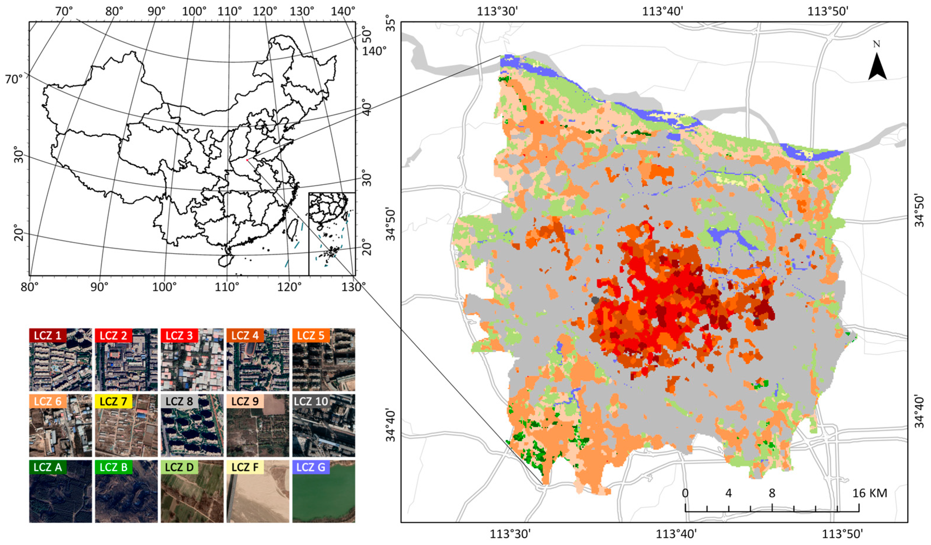
2.1. Research Area and LCZ Classification

Zhengzhou, the capital of Henan Province in central China, is situated in the Yellow River Valley, featuring flat terrain bordered by the Yellow River to the north and the Songshan Mountains to the southwest (Figure 2). The city has a humid subtropical climate with distinct seasons, including hot, humid summers and cold, dry winters. Vegetation resources are mainly concentrated in urban parks and along riverbanks, providing localized cooling effects that help mitigate the SUHI effect. However, water resources in the region are limited, with the Yellow River serving as the primary water body. In recent decades, rapid urbanization has significantly reshaped the city, with the urbanization rate reaching 70% by 2022. The central districts—Jinshui, Erqi, Zhongyuan, Huiji, and Guancheng Hui—span 550 square kilometers and house dense populations (~1200 people/km²). These densely developed areas, strongly influenced by the SUHI effect, provide an ideal setting for analyzing spatial variations in land surface temperature (LST).

The LCZ classification system was used to categorize the study area. Through the LCZ Generator, a detailed classification of urban and natural land cover types was created [14,17]. The LCZ classification divides Zhengzhou’s main urban area into built-type LCZ (LCZ 1–10) and non-built-type LCZ (LCZ A, B, D, F, G) (

Table 1. LCZ classification.

	LCZ	Definitions	Area (km2)
Built type	1	Compact highrise	14.23
	2	Compact midrise	39.1
	3	Compact lowrise	0.66
	4	Open highrise	51.04
	5	Open midrise	36.38
	6	Open lowrise	144.97
	7	Lightweight lowrise	0.06
	8	Large lowrise	483.59
	9	Sparsely built	81.7
	10	Heavy industry	0.96
Non-built type	A	Dense trees	3.47
	B	Scattered trees	4.66
	D	Low plants	129.9
	F	Bare soil or sand	4.4
	G	Water	23.41

). Notably, Zhengzhou lacks LCZ C (bush/scrub) and LCZ E (bare rock or paved), and the sample size for LCZ 7 (lightweight lowrise buildings) is insufficient for meaningful analysis and will not be discussed further.

2.2. LST Calculation and Accuracy Assessment

Landsat 8 and Landsat 9 Thermal Infrared Sensor (TIRS) imagery was used to retrieve LST for Zhengzhou throughout 2022. Images with cloud cover below 10% were selected, resulting in 24 suitable datasets spanning 1 January to 31 December 2022. The mean LST derived from these images was calculated to represent the annual LST for the study area. Data processing was conducted on the Google Earth Engine platform using the Single Channel Algorithm, ensuring consistent and reliable LST retrieval [18,19].

To assess LST variations across different LCZs, the Tamhane T2 test was applied, revealing significant distinctions in LST among zones. Accuracy was evaluated using the root mean square error (RMSE) method by comparing satellite-derived LST values with ground-based temperature measurements from meteorological stations. This validation process confirmed the accuracy and reliability of the LST retrieval, providing a robust basis for analyzing LST distribution and its driving factors across Zhengzhou’s LCZs.

2.3. Explanatory Variables

To explain the variation in LST across different LCZs, 30 explanatory variables were selected, representing factors with potential direct or indirect effects on LST (

Table 2. Description of explanatory variables.

Category	Variable	Abbr.	Description	Data Sources
Vegetation Characteristics Indices	Number of Trees	Ntree	Total count of trees within the sample plots.	Field research
	Average Diameter at Breast Height	DBHtree	Average diameter of tree trunks at 1.3 m above the ground.
	Average Height of Trees	Htree	Mean height of trees in the sample plots.
	Average Crown Width of Trees	CWtree	Mean width of the tree crowns.
	Number of Shrubs	Nshrub	Total count of shrubs within the sample plots.
	Average Height of Shrubs	Hshrub	Mean height of shrubs in the sample plots.
	Average Base Diameter of Shrubs	BDshrub	Average diameter of the shrub bases.
	Menhinik Richness	Dmn	Species richness, normalized by the square root of the total number of individuals.
	Simpson Degree of Dominance	D	Measure of species dominance and evenness.
	Pielou’s Uniformity	J	Evenness of species distribution.
Urbanization Indices	Population Density	PD	Number of people per unit area.	[20]
	Nighttime Light Data	NPP_VIIRS	Intensity of nighttime lights, indicating economic activity and urbanization.	[21,22]
	Per Capita GDP	GDP	Average economic output per person.	[23]
	Road Density	RD	Length of roads per unit area.	[24]
	Building Average Height	BH	Average height of buildings.	[25]
	Building Density	BD	Number of buildings per unit area.	[24]
Climatic Indices	Solar Radiation	SR	Amount of solar energy received per unit area.	Calculation based on Landsat data
	Precipitation	PR	Total rainfall received.	[26]
	Evaporation	EV	The amount of water evaporated from the surface.	Calculation based on Landsat data
	Aridity index	AI	Measure of the degree of dryness in a region.	[26]
Tasseled Cap Transformation Indices	Greenness	TCG	Indicator of vegetation abundance and health.	Calculation based on Landsat data
	Wetness	TCW	Indicator of soil moisture and water content.
	Brightness	TCB	Indicator of the brightness of surfaces, reflecting their heat absorption and retention properties.
Landscape Pattern Indices	Percentage of Landscape	PLAND	Proportion of the landscape covered by a specific land cover type.	Calculation based on Landsat data
	Number of Patches	NP	Count of distinct patches of a specific land cover type.
	Total Core Area	TCA	Sum of the core areas of patches, excluding edge effects.
	Normalized Difference Core Area	NDCA	Core area adjusted for the size of the landscape.
	Total Edge Contrast Index	TECI	Measure of the contrast between different land cover types along their edges.
	Landscape Cohesion Index	COHESION	Degree to which the landscape is physically connected.
	Splitting Index	SPLIT	Measure of landscape fragmentation.

). These variables were categorized into five groups: vegetation characteristics indices, urbanization indices, climatic indices, Tasseled Cap Transformation indices, and landscape indices. This categorization aimed to comprehensively capture the diverse influences on LST and support a robust analysis of their impacts. All variables were resampled to a consistent 100 × 100 m grid to ensure uniform spatial resolution across the dataset. Covariance diagnostics were conducted to assess multicollinearity within each group, with the Variance Inflation Factor (VIF) employed to identify and address multicollinearity, thereby enhancing the reliability of the subsequent analyses. To further investigate the differences in driving factors across LCZs, Analysis of Variance (ANOVA) was applied.

This study tailored the inclusion of explanatory variables based on the specific characteristics of different LCZ types. For non-built type LCZs (e.g., A, B, D, F, and G), vegetation characteristic indices were excluded due to the predefined vegetation coverage of these zones. For example, LCZ A (dense trees) is predominantly covered by high-density tree vegetation, rendering shrub-related features (e.g., shrub count or average height) less relevant. Similarly, the aquatic nature of LCZ G eliminates the applicability of urbanization indices (e.g., building density, population density, and nighttime light intensity). By excluding irrelevant indicators, the analysis maintains scientific rigor and logical consistency, ensuring that the results accurately reflect the dominant driving factors specific to each LCZ type.

2.3.1. Vegetation Characteristics Indices

Vegetation data were collected through field surveys conducted during the summer of 2022. A total of 1153 sample plots, each measuring 20 × 20 m, were surveyed to comprehensively assess the vegetation structure in the central region of Zhengzhou. These plots captured detailed information on both the arboreal and shrub components of urban vegetation.

For the arboreal layer, the recorded indices included the number of trees, average diameter at breast height (DBH), average tree height, and average crown width. These parameters collectively characterize the density, size, and vertical structure of the tree layer. For the shrub layer, data were collected on the number of shrubs, average shrub height, and average base diameter, providing essential insights into shrub density and structural composition.

To assess biodiversity and its potential role in influencing the SUHI effect, three biodiversity indices were calculated: Menhinik Richness Index (Dmn) quantifies species richness while adjusting for variations in sample size [27]. It provides a robust measure of the diversity of species within a given area (Equation (1)). Simpson Degree of Dominance (D) index measures the probability that two randomly selected individuals belong to the same species, reflecting species dominance and evenness [28] (Equation (2)). Pielou’s Uniformity Index (J) metric evaluates the evenness of species distribution, indicating how uniformly individuals are distributed among species within a community [29,30] (Equation (3)).

$$Dmn={\displaystyle \frac{S}{\sqrt{N}}}$$

(1)

$$D=\sum _{i=1}^S{P}_i^2$$

(2)

$$J={\displaystyle \frac{-{\sum }_{i=1}^S{p}_i\ln \left(p_i\right)}{\ln \left(S\right)}}$$

(3)

where $S$ represents the total number of species, $N$ is the total number of individuals recorded, $P_i$ and is the proportional abundance of the $i$-th species. These vegetation characteristics and biodiversity metrics provide a comprehensive understanding of the structural and ecological features of urban vegetation, offering critical insights into their role in shaping the thermal environment in Zhengzhou.

2.3.2. Urbanization Indices

Urbanization indices were selected to reflect human activities and urban spatial characteristics. Demographic and economic factors were represented by population density, nighttime light data, and per capita GDP. Building and road density were calculated using OpenStreetMap data: building density was determined by the proportion of building footprints within each 100 m grid, while road density was derived from the total length of highways (including motorway, trunk, primary, secondary, tertiary, residential, track, and unclassified roads) within the same grid.

2.3.3. Climatic Indices

Climatic indices included solar radiation, evaporation, precipitation, and atmospheric dryness. Solar radiation and evaporation were calculated using Landsat 8 and 9 images (LANDSAT/LC08/C02/T1_L2 and LANDSAT/LC09/C02/T1_L2) on Google Earth Engine. Precipitation data were sourced from Peng et al. (2019), and atmospheric dryness was obtained from [26].

2.3.4. Tasseled Cap Transformation Indices

Tasseled Cap Transformation indices [31]—Greenness, Wetness, and Brightness—were also derived from the same Landsat 8 and 9 images as above. These indices, calculated using the Tasseled Cap Transformation method, captured vegetation abundance, soil moisture, and surface brightness, offering key insights into land cover characteristics influencing LST.

2.3.5. Landscape Indices

Landsat 8 imagery from the summer months (June to September) of 2022, with cloud cover of less than 5%, was selected and mosaicked into a single image for analysis based on 5 suitable datasets. The study area was classified into five land use types—impervious surfaces, green spaces, cropland, bare soil, and water bodies—using the maximum likelihood classification algorithm. Landscape pattern indices for impervious surfaces were then computed at the class level using Fragstats 4.2 software. Following collinearity diagnostics, the landscape metrics retained for further analysis are presented in Table 2.

2.4. Statistical Analysis

To investigate the relationship between LST and the selected explanatory variables, this study adopted a systematic analytical framework that integrates statistical methods and machine learning techniques.

First, the Spearman Correlation Coefficient was calculated to quantify nonlinear relationships between LST and the explanatory variables across different LCZs. Significant correlations (p < 0.01 or p < 0.05) were identified to determine the variables with the most substantial impact on LST, providing a foundation for understanding initial relationships between LST and its drivers.

Next, the boosted regression trees (BRTs) model was applied to explore the relative importance of driving factors in explaining LST variations across LCZ categories and subcategories. By combining regression trees with boosting techniques, the BRT model iteratively builds multiple models to improve predictive accuracy. This approach effectively captures complex nonlinear relationships and interactions between explanatory variables and LST [32]. Key drivers with significant explanatory power for LST variations in different LCZs were identified through this analysis.

Finally, to further evaluate the explanatory power of critical driving factors, a random forest model [33] was employed across various LCZ categories. Partial dependence analysis was conducted to provide a clearer understanding of the independent effects of key variables. Partial dependence plots were generated to visually demonstrate the influence of individual variables on LST trends, holding other variables constant. These plots revealed the direction and proportional impact of each variable on LST, offering robust evidence for the mechanisms driving LST variations.

3. Results

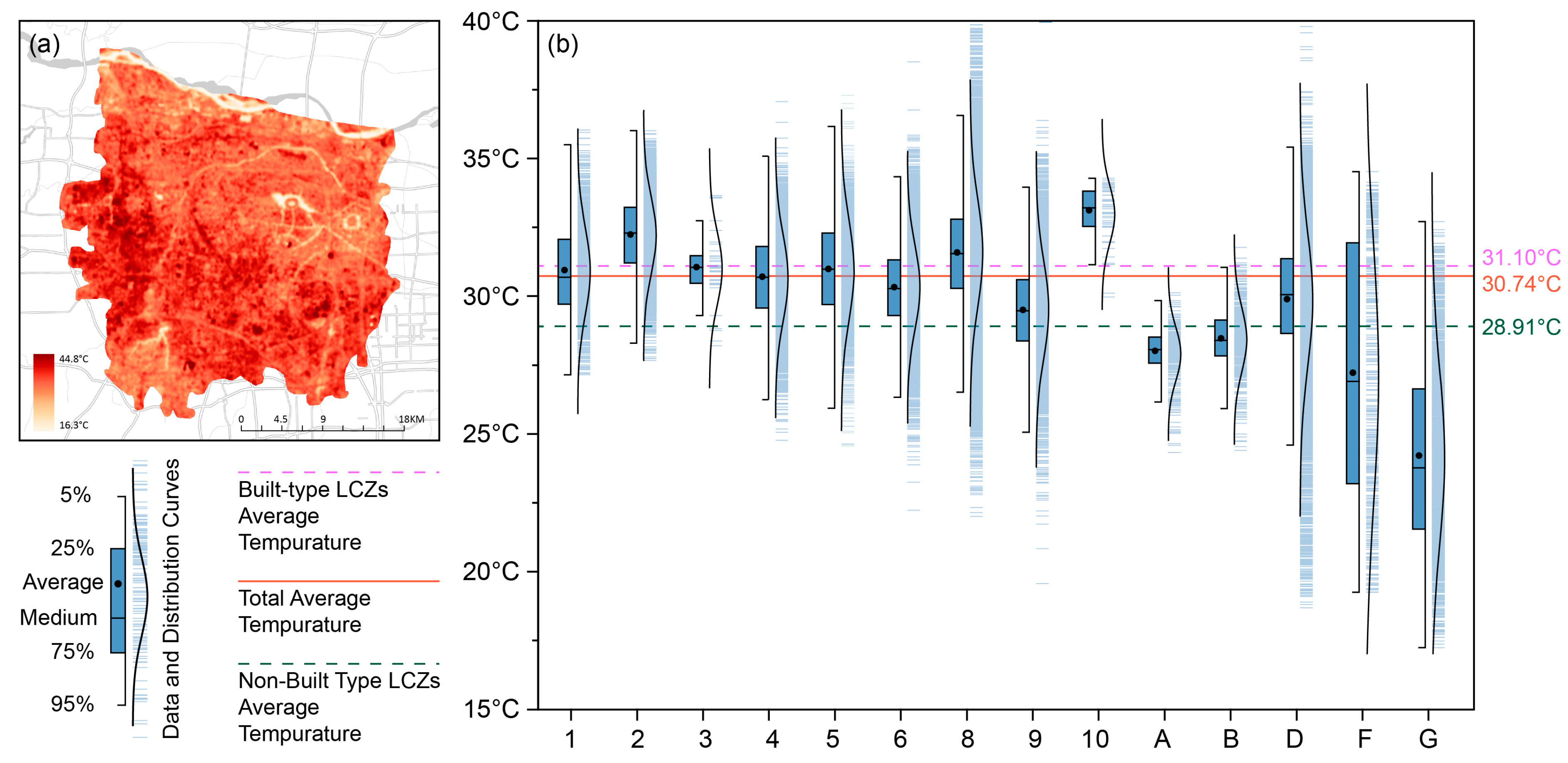
3.1. Variation of LST in Different LCZs

The LST distribution across various LCZs in Zhengzhou exhibited substantial variability (Figure 3). The city-wide average LST was calculated as 30.74 °C, with notable differences between building-dominated LCZs (LCZs 1–10) and non-building-dominated LCZs (LCZs A, B, D, F, and G). Building-dominated LCZs showed a higher mean LST of 31.10 °C, with individual zones ranging from 27.04 °C to 35.15 °C and a standard deviation of 2.86 °C. In contrast, non-building-dominated LCZs displayed a lower mean LST of 28.91 °C, with values ranging from 21.88 °C to 34.13 °C and a standard deviation of 3.26 °C.

Significant thermal differences were also observed within the same LCZ category. For instance, LCZ 8 exhibited an interquartile range of 2.86 °C, with LST values spanning from 30.35 °C to 33.20 °C. In comparison, LCZ 7 showed a narrower interquartile range of 0.43 °C, with temperatures varying from 31.96 °C to 32.39 °C. Among non-building-dominated LCZs, LCZ D demonstrated higher temperature peaks, with a mean LST of 30.14 °C and a maximum of 34.47 °C, while LCZ G consistently maintained cooler temperatures, with a mean LST of 24.49 °C and a minimum of 17.48 °C.

3.2. Differences in Driving Factors Across Different LCZs

The analysis of normalized mean values for driving factors across LCZs reveals significant spatial variations, reflecting the interplay between urban and natural characteristics in shaping LST (Figure 4).

Vegetation characteristics indices exhibit distinct patterns across LCZs, with dense urban zones such as LCZs 1, 2, and 3 showing similar vegetation profiles, while suburban zones (LCZs 4 and 5) and industrial areas (LCZs 6 and 9) form separate clusters. These differences highlight the varying density and structural composition of vegetation in different urban contexts.

Urbanization indices, including population density (PD), nighttime light intensity (NPP_VIIRS), and building density (BD), are significantly elevated in built-type LCZs, particularly LCZs 1, 2, and 3. For example, PD peaks in LCZ 2 but drops to zero in non-built type LCZ F. Similarly, NPP_VIIRS reaches its highest value in LCZ 1, emphasizing its role as a central urban hub, while LCZ A exhibits minimal values, characteristic of less urbanized environments. These trends underscore the intensity of human activities in Built-Type LCZs compared with their non-built counterparts.

Climatic indices also display notable variations. LCZs 1–5 show higher levels of solar radiation (SR) and precipitation (PR), while evaporation (EV) and aridity index (AI) are comparatively low, reflecting the influence of urban microclimates. In contrast, non-built LCZs exhibit elevated EV and AI, which is indicative of the cooling and moisture-retaining effects of natural land cover.

Landscape pattern indices reveal substantial differences in fragmentation and heterogeneity across LCZs. The number of patches (NPs) is highest in LCZ 6, reflecting diverse land use patterns, and lowest in LCZ 2, indicative of a homogeneous urban landscape. Meanwhile, the Splitting Index (SPLIT), which measures landscape fragmentation, peaks in LCZ A, highlighting the fragmented nature of rural and natural zones compared with the compactness of urban areas.

3.3. Spearman Correlation Analysis

The results showed that vegetation characteristics indices had weak overall correlations with LST but exhibited significant influences in certain LCZs (Figure 5). Tree-related indices, such as Ntree, DBHtree, Htree, and BDshrub, demonstrated strong correlations with LST in LCZ 1. Additionally, shrub-related indices, including Nshrub, Hshrub, and BDshrub, were generally positively correlated with LST across various LCZs, while biodiversity indices (Dmn, D, and J) were predominantly negatively correlated with LST.

Urbanization Indices exerted widespread effects on LST but displayed moderate overall correlations. In built-type LCZs, PD, RD, and BD were generally positively correlated with LST, while NPP_VIIRS, GDP, and BH exhibited negative correlations in the same zones. Conversely, in non-built-type LCZs, urbanization indices were predominantly positively correlated with LST, particularly in LCZ F. When considered across broader categories, such as all built-type LCZs, non-built-type LCZs, or total LCZs, all six urbanization indices consistently showed positive correlations with LST.

Climatic Indices exhibited significant correlations with LST across nearly all LCZs except LCZ 3. Most climatic indices were negatively correlated with LST, but AI showed a significant positive correlation with LST in the overall non-built-type LCZs. Similarly, Tasseled Cap Transformation indices displayed stronger correlations with LST in non-built-type LCZs compared with built-type LCZs. TCB was generally positively correlated with LST across most LCZs, whereas TCG and TCW were mostly negatively correlated with LST but exhibited positive correlations in LCZ D and LCZ F.

The relationships between landscape pattern indices and LST were more complex and varied across LCZs. While most landscape pattern indices exhibited significant correlations with LST in different LCZs, these correlations were weak or insignificant in LCZ A and LCZ B. At broader scales, including total LCZs, built-type LCZs, and non-built-type LCZs, LST showed positive correlations with PLAND, TCA, NDCA, and COHESION, while negative correlations were observed with TECI and SPLIT.

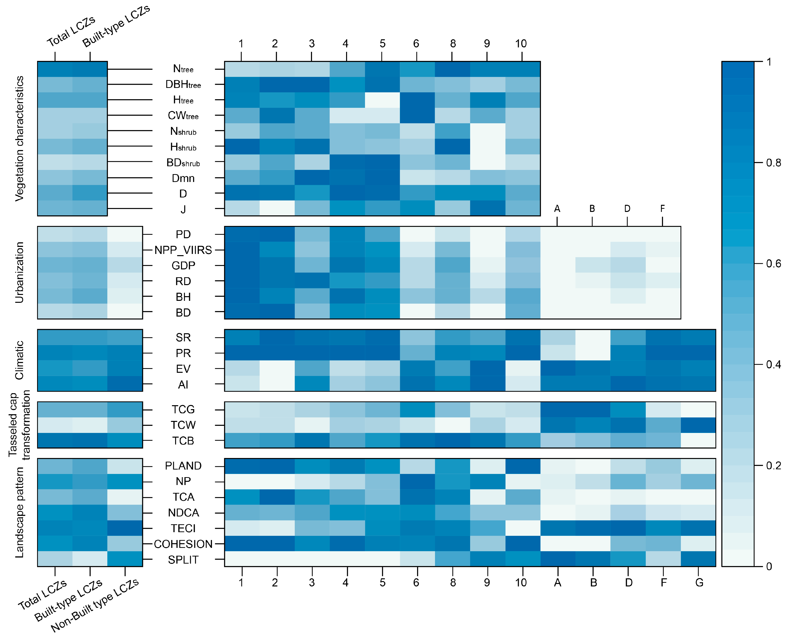
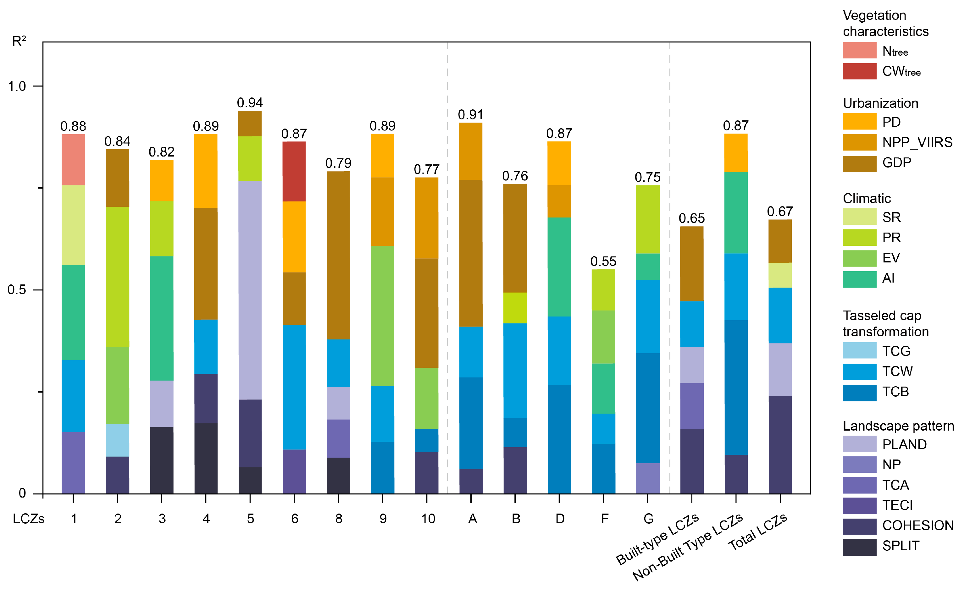
3.4. Relative Importance of Factors

Figure 6 illustrates the relative importance of driving factors in explaining LST variations across different LCZs, revealing substantial differences in their effects. Overall, landscape pattern indices emerged as the dominant driving factors for built-type LCZs, accounting for 44.5% of the total explanatory power, followed by urbanization indices, which contributed 26.4% (Figure 6a). In contrast, Tasseled Cap Transformation Indices were the most influential for non-built-type LCZs, explaining 42.8% of the variation. For the entire study area of Zhengzhou, landscape pattern indices remained the most significant category, contributing 41.7%, followed by urbanization indices (24.7%), Climatic Indices (13.0%), and Tasseled Cap Transformation Indices (12.7%).

A more detailed analysis of individual categories (Figure 6b–f) highlights the key variables within each type of driving factor and their varying levels of importance. Among vegetation characteristics indices, Nshrub contributed the most to LST variations (19.6%), followed by tree-related indices such as Htree (16.1%) and Ntree (13.4%), whereas biodiversity indices had relatively lower explanatory power. Within urbanization indices, GDP per capita (41.1%) and NPP_VIIRS (29.7%) were identified as the most significant contributors. Climatic Indices and Tasseled Cap Transformation Indices demonstrated relatively even contributions across variables, with solar radiation (SR) accounting for 33.9% of Climatic Indices and Wetness (TCW) dominating Tasseled Cap Transformation Indices at 49.0%. For landscape pattern indices, the key drivers varied across LCZs, but COHESION (21.9%) and PLAND (20.2%) generally stood out as the most significant.

Figure 7 further delineates the key driving factors for each LCZ and their total explanatory power. The explanatory power of key factors ranged from 0.65 to 0.94, underscoring their substantial influence on LST variations. Landscape pattern indices dominated the LST driving mechanisms in built-type LCZs and across all LCZs, while non-built-type LCZs were more strongly influenced by Tasseled Cap Transformation Indices, particularly TCB, a pattern also evident in LCZ D and LCZ G. Within specific subcategories of built-type LCZs, the dominant drivers varied significantly. For example, LCZs 1, 2, and 9 were primarily influenced by Climatic Indices, and LCZs 4 and 8 were more affected by urbanization indices, while LCZs 5 and 6 were predominantly driven by landscape pattern indices and Tasseled Cap Transformation Indices, respectively.

In summary, the relative importance of LST driving factors exhibited significant spatial heterogeneity across different LCZs. This heterogeneity reflects the combined effects of natural conditions and human activities, providing a basis for targeted LST regulation strategies and emphasizing the necessity of differentiated management approaches.

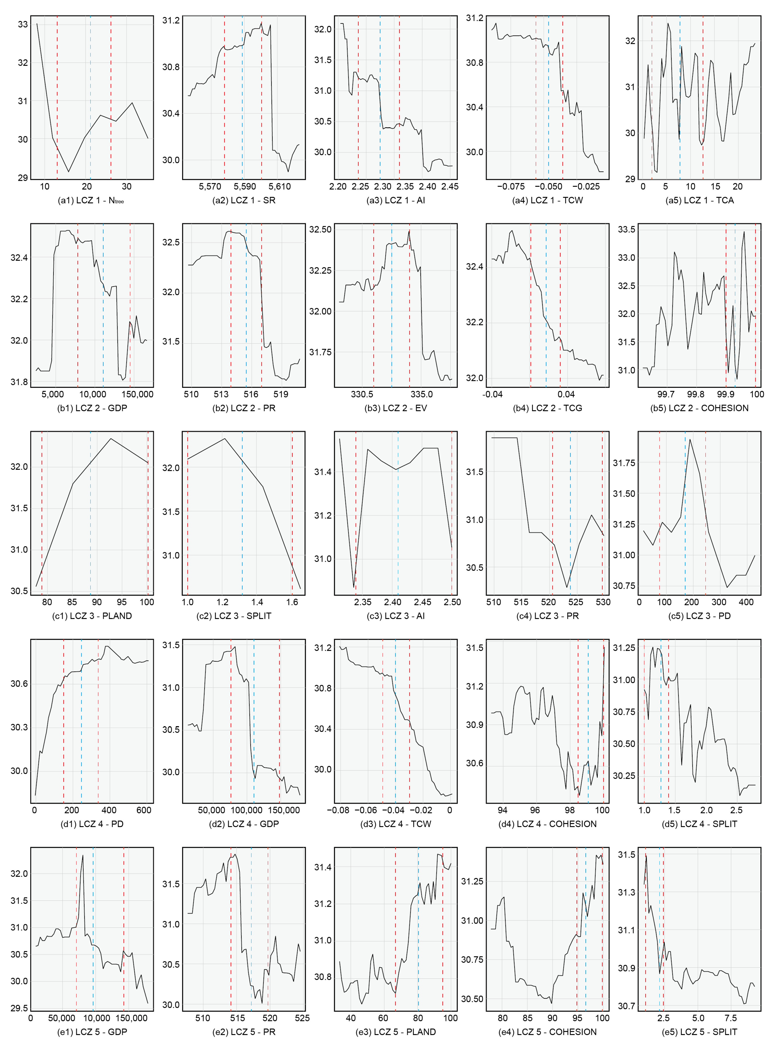
3.5. Partial Dependence Analysis of Key Driving Factors

Partial dependence analysis provides deeper insights into the influence of individual driving factors on LST variations across different LCZs (Figure 8 and Appendix A). For all built-type LCZs, key factors primarily influence cooler areas. Increases in TCW and SPLIT are associated with cooling effects, whereas GDP, COHESION, and PLAND contribute to warming.

In the whole, non-built-type LCZs, COHESION, PD, and TCB play significant roles in driving temperature increases, while higher levels of TCW and AI are linked to notable cooling effects. Across the total LCZs, PLAND and GDP emerge as strong contributors to warming, whereas SR and TCW effectively mitigate thermal effects. Notably, COHESION exhibits a nonlinear relationship with LST, initially suppressing temperature increases before eventually promoting them.

4. Discussion

4.1. The LST Under Different LCZs

This study reveals significant differences in LST both between different LCZs and within the same LCZ types. These differences reflect not only the spatial variation in surface energy balance [34,35], such as the heat absorption and release characteristics of impervious surfaces [36], but also the combined effects of vegetation cover [8,37], water body evaporation cooling [38], and building morphology on local microclimates [39].

Between LCZs, the average LST in built-type LCZs is significantly higher than that in non-built-type LCZs (31.10 °C vs. 28.91 °C). This finding aligns with previous studies [40,41]. For example, Zwolska et al. reported that in Poznań, transitioning from a non-built LCZ to a built LCZ can increase LST by up to 1.19 °C, while transitioning from a compact LCZ to an open LCZ can decrease LST by 0.70 °C [42]. This phenomenon is likely due to the lower albedo and higher specific heat capacity of urban impervious surfaces [8,43]. Additionally, differences in building density and materials further exacerbate the SUHI effect by altering surface heat storage and heat conduction properties. For instance, high-density areas often trap heat due to restricted ventilation [44], while low-albedo materials such as asphalt or concrete absorb more solar radiation, significantly increasing local temperatures [45].

Among built-type LCZs, LCZ 10 exhibited the highest LST, consistent with findings by Li et al. in Shenyang [46]. However, Wang et al. observed that in the Pearl River Delta, LCZ 4 and LCZ 6 are typically the built LCZs with the highest LST [47]. These regional differences may be attributed to the higher humidity in the Pearl River Delta, which creates a shielding effect on heat transfer [48], as well as its more open building layout, which alters heat distribution patterns compared with inland cities [49]. Furthermore, Žgela et al. noted that LCZ 9 generally has the lowest LST among built LCZs in inland cities [41]. This aligns with the findings of this study, where LCZ 9 in Zhengzhou had a median LST of 29.89 °C. Possible reasons include the diverse surface coverage in LCZ 9, such as the presence of large open spaces, bare soil, and temporary green areas in light industrial zones, which generally exhibit lower surface temperatures. Additionally, the sparsely built structures in LCZ 9 are typically lower in height, reducing the potential for heat accumulation.

Among non-built-type LCZs, LCZ D (low plants) recorded the highest LST, with a peak value of 34.47 °C. This may be due to the distribution of low vegetation, primarily among sparse buildings, which are significantly influenced by heat radiation from the structures. Furthermore, the low density and canopy height of the vegetation limit its cooling effect. In contrast, LCZ G (water bodies) typically has the lowest LST among non-built-type LCZs [50], as water bodies have high specific heat capacity and provide evaporative cooling. This pronounced LST gradient indicates that even within non-built LCZs, surface characteristics have a significant impact on LST.

Moreover, the range of LST distribution in built-type LCZs is notably narrower compared with non-built LCZs [51], with the average LST fluctuation being 6.76 °C in built LCZs, versus 10.48 °C in non-built LCZs. The internal LST differences in LCZ D, F, and G are particularly pronounced. In LCZ D, small changes in the proportion of low vegetation and bare soil can significantly influence LST. LCZ F (bare soil) is strongly affected by soil moisture [52] and surface roughness, with LST variations exceeding 3 °C across different areas. In LCZ G, variations in water depth, pollution levels, and surrounding green space proportions may also significantly impact its internal LST gradients [53].

4.2. Driving Factors of LST

This study reveals significant differences in the driving factors of LST across different LCZs, reflecting the combined effects of natural conditions [54] and human activities [12,55]. These differences highlight the complexity of urban thermal environments and provide scientific evidence for differentiated SUHI mitigation strategies.

In built-type LCZs, urbanization indices and landscape pattern indices are the primary influencing factors. This is likely because urban centers concentrate on socio-economic activities (e.g., commerce, industry, and transportation) that generate anthropogenic heat, directly increasing local LST [56]. Meanwhile, high PLAND values, representing extensive impervious surfaces, directly result in the loss of evapotranspiration cooling effects and enhance LST through increased absorption of solar radiation. For example, the study by Coseo and Larsen pointed out that for every 10% increase in the impervious surface area of a neighborhood, the air temperature in the community rises by 0.97 °C at 2 a.m. [57]. High connectivity of impervious surfaces or large building clusters often limits natural ventilation, creating heat accumulation zones and leading to elevated LST. Conversely, fragmented landscape structures (e.g., high SPLIT and TECI values) facilitate heat dissipation and enhance airflow, promoting heat exchange and thereby alleviating thermal stress to some extent [58].

Furthermore, in densely built-up zones (LCZ1, 2, 3), the relative importance of climatic factors is significantly higher. As previously noted, ventilation in these areas is restricted by building density and height, impeding airflow and allowing heat to accumulate [59]. Under such conditions, climatic factors (e.g., SR, EV, and AI) exert a more pronounced influence on LST. For instance, high SR and low EV exacerbate thermal stress in dense urban areas [60], while increased AI may further reduce the cooling effects of vegetation and open spaces. Additionally, high heat-capacity materials (e.g., concrete and asphalt) used in dense built-up areas respond more directly to climatic factors. These materials’ thermal properties (e.g., high heat storage and low reflectivity) amplify the impact of climatic factors on LST, making them “amplifiers” of local climate variations [61,62].

In the transition from LCZ A to LCZ F, the influence of urbanization factors on LST gradually diminishes, while the role of climatic factors becomes increasingly dominant. This shift reflects a fundamental transition in LST driving mechanisms driven by changes in vegetation coverage.

In high vegetation coverage zones (e.g., LCZ A and B), urbanization factors significantly impact LST, primarily through artificial irrigation [63], landscaping [64], and other urbanization activities that directly affect vegetation’s evapotranspiration efficiency and shading effects, thereby indirectly regulating LST. For instance, artificial irrigation enhances evapotranspiration, while landscaping optimizes vegetation structure to improve cooling efficiency. These human interventions considerably alter LST dynamics in these areas, making urbanization factors more influential.

However, as the transition progresses from LCZ A to LCZ F, the decline in vegetation coverage weakens the indirect regulation of LST by urbanization factors. In moderately vegetated zones (e.g., LCZ D), urbanization factors still influence vegetation to some extent, but LST is increasingly driven by surface physical properties (e.g., TCW and TCB) rather than human interventions. Sparse and dispersed vegetation in these areas limits the impact of human activities such as irrigation or management, significantly weakening vegetation’s cooling effect. Additionally, the rising proportion of impervious surfaces shifts thermal regulation towards surface thermodynamic properties. For example, bare surfaces with high heat capacity and low reflectivity enhance the direct influence of solar radiation on LST, further diminishing the role of urbanization factors.

In low vegetation or bare soil zones (e.g., LCZ F), the influence of urbanization factors on LST becomes negligible. This is because the thermophysical properties of bare surfaces (e.g., high heat capacity and low reflectivity) dominate LST dynamics, and natural climatic factors (e.g., solar radiation and precipitation) play a more direct role. Under such conditions, intense solar radiation directly raises LST, while the absence of vegetation eliminates evapotranspiration cooling effects, making LST entirely dependent on natural climatic factors and surface properties. Socio-economic activities (e.g., land use) have limited capacity to modify bare surfaces, and activities such as road construction or further land exposure often exacerbate thermal stress [65].

4.3. Implications for Future Urban Planning and Management

For built-type LCZs, priority should be given to optimizing landscape patterns. Increasing green infrastructure and enhancing landscape connectivity can effectively mitigate SUHI effects. For non-built-type LCZs, the focus should shift to soil moisture management and balanced vegetation configuration to maximize cooling effects and improve microclimate conditions.

In built-type LCZs, the high density and height of buildings are major constraints. Optimizing building layouts to create more open urban forms, such as designing ventilation corridors to promote airflow and incorporating small open spaces in dense areas, can help reduce heat accumulation. The use of high-reflectivity materials like cool roofs and walls, along with phase-change materials to balance day-night temperature fluctuations, offers further cooling potential. Vertical greening solutions, such as green walls and roofs, can enhance vegetation coverage without additional land use, effectively mitigating urban heat stress.

In vegetation-dominated LCZs, the emphasis should be on protecting and enhancing vegetation functionality. Reducing excessive human intervention, such as over-pruning, can allow natural vegetation to strengthen its ecological regulatory role [66]. Optimized irrigation systems can balance water use while maximizing the cooling effects of vegetation transpiration [67]. Addressing green space fragmentation through the establishment of ecological corridors can ensure connectivity while introducing drought-resistant vegetation, which can enhance adaptability to high temperatures and sustain cooling performance under low-precipitation conditions.

For LCZs with low vegetation or bare surfaces, such as LCZ F, strategies should focus on restoring shading and transpiration effects by introducing grass, shrubs, or drought-resistant plants. Bare surfaces can be multifunctionally transformed by integrating green infrastructure, permeable pavements, or solar panels to reduce heat absorption while adding environmental benefits [68]. The inclusion of water features, such as rain gardens or artificial lakes, can also effectively regulate local microclimates. Where vegetation establishment is not feasible, light-colored or reflective materials can be applied to mitigate heat stress on exposed surfaces.

In mixed LCZs, such as LCZ 9 and LCZ D, the focus should be on optimizing surface structure and enhancing functionality. Increasing the proportion of permeable surfaces using materials like grass pavers or permeable concrete can improve cooling efficiency. Multifunctional green infrastructure, such as community parks or rainwater management systems, can enhance the area’s thermal regulation capabilities. Diversifying land-use layouts by integrating farmland, vegetation, and built-up areas can create favorable microclimate conditions for heat dissipation and enhance overall regional adaptability.

Overall, implementing effective cooling strategies for different LCZs requires the use of high-resolution LST monitoring data to dynamically evaluate intervention outcomes and make necessary adjustments. Interventions should prioritize areas most sensitive to LST changes to maximize impact. Policy guidance and public participation play critical roles in improving implementation efficiency. Promoting urban greening policies, supporting the adoption of energy-efficient building technologies, and encouraging community involvement in afforestation and green space maintenance are essential steps. By adopting scientifically informed and differentiated management strategies, urban areas can significantly improve thermal environments and mitigate the SUHI effect, providing a sustainable pathway for future urban development.

4.4. Limitations and Future Prospects

Despite analyzing the key drivers of LST within LCZs in Zhengzhou by integrating ground surveys and remote sensing data, this study has certain limitations, which also point to potential directions for future research.

First, this study focused solely on Zhengzhou, a case city that, while representative of rapid urbanization, may limit the generalizability of the findings. For instance, Bechtel et al. noted significant spectral differences within the same LCZ classifications across different regions [69]. Expanding the study to cities in diverse climatic contexts (e.g., arid, humid, or coastal regions) could help reveal the diversity of LST driving mechanisms under different environmental conditions. Second, this study primarily analyzed the annual mean LST, neglecting potential seasonal variations in LST drivers. He et al. highlighted the ability of LCZ classifications to capture urban thermal environment differences across seasons [70]. Seasonal variations could significantly alter the weight of LST drivers, suggesting that future research should incorporate seasonal or even finer diurnal data to explore the dynamic patterns of LST. Third, the boundary effects between different LCZs have not been fully quantified. Thermal spillover effects across LCZs may create complex thermal interactions between adjacent zones. While Vaidya et al. proposed a spatial heterogeneity framework, this study falls short in exploring such dynamics [71]. Additionally, this study derived LST solely from remote sensing data, which may introduce uncertainties due to the lack of ground-based validation.

To address these limitations, future research can advance in several directions. First, cross-regional comparative studies involving multiple cities and climatic contexts are essential. Integrating urban case studies from varying climate zones and urbanization patterns could enhance the understanding of the global applicability of the LCZ framework. For instance, comparing LST drivers in arid versus humid cities could help identify universal mechanisms for regulating urban thermal environments under global change scenarios. Second, seasonal analyses should be incorporated to uncover temporal dynamics. Leveraging high-temporal-resolution remote sensing or field monitoring data could elucidate seasonal and even diurnal shifts in LST drivers. For example, Zwolska et al. (2024) demonstrated significant differences in LST drivers between winter and summer in their analysis of the SUHI effect in Polish cities, highlighting the value of seasonal data [42]. Peng et al. found that in summer, transitional seasons, and winter, the most explanatory variables for LST changes were the normalized difference built-up index, normalized difference vegetation index, and construction land percentage, with explanatory power of 53.62%, 47.84%, and 26.84%, respectively [72]. These findings underline the importance of temporal analysis in understanding thermal environments.

Furthermore, future research should emphasize boundary effects and spillover dynamics between LCZs. High-precision spatial statistical methods could be employed to investigate the thermal interactions between adjacent LCZs, thereby deepening understanding of intra-urban thermal dynamics. Lastly, integrating machine learning techniques and urban climate simulation models could uncover the complex interactions among drivers. Deep learning methods could analyze nonlinear relationships in multidimensional data, while simulation models could predict LST variations under different urban planning scenarios, providing valuable data support for policy-making. Finally, to enhance the accuracy of the research, future studies could integrate multi-source data, such as local meteorological observations, to cross-validate satellite-derived LST.

5. Conclusions

This study employed the LCZ framework to analyze the spatial variability of LST and its driving factors in Zhengzhou, China, using 2022 Landsat imagery. Machine learning regression models, including boosted regression trees and random forests, along with partial dependence analysis, were applied to examine the nonlinear relationships between LST and 30 potential drivers, such as vegetation characteristics, urbanization, climatic conditions, tasseled cap indices, and landscape patterns. The findings revealed spatial heterogeneity in LST drivers, underscoring the importance of integrating LCZ-specific mitigation strategies into urban planning.

Results indicated that built-type LCZs (LCZ 10 > 2 > 8 > 3 > 5 > 1 > 4 > 6 > 9) exhibited significantly higher LSTs compared with non-built LCZs (LCZ D > B > A > F > G), which demonstrated greater spatial heterogeneity. Landscape indices and tasseled cap indices were identified as the primary drivers for built-type and non-built LCZs, respectively, while vegetation characteristics contributed minimally to LST variations. Random forest models effectively explained the relationship between drivers and LST within the LCZ framework, with explanatory power ranging from 0.65 to 0.94. Mitigation strategies should prioritize optimizing urban morphology, expanding green infrastructure, and enhancing landscape connectivity in built-type LCZs to reduce heat accumulation. In non-built LCZs, efforts should focus on maintaining soil moisture, optimizing vegetation configurations, and addressing microclimatic factors such as evapotranspiration and solar radiation to amplify cooling effects.

References

1. Kim, S.W.; Brown, R.D. Urban Heat Island (UHI) Intensity and Magnitude Estimations: A Systematic Literature Review. Sci. Total Environ. 2021, 779, 146389. [Google Scholar] [CrossRef] [PubMed]
2. Meng, Q.; Zhang, L.; Sun, Z.; Meng, F.; Wang, L.; Sun, Y. Characterizing Spatial and Temporal Trends of Surface Urban Heat Island Effect in an Urban Main Built-up Area: A 12-Year Case Study in Beijing, China. Remote Sens. Environ. 2018, 204, 826–837. [Google Scholar] [CrossRef]
3. Shi, L.; Ling, F.; Foody, G.M.; Yang, Z.; Liu, X.; Du, Y. Seasonal SUHI Analysis Using Local Climate Zone Classification: A Case Study of Wuhan, China. Int. J. Environ. Res. Public Health 2021, 18, 7242. [Google Scholar] [CrossRef]
4. Tao, F.; Hu, Y.; Tang, G.; Zhou, T. Long-Term Evolution of the SUHI Footprint and Urban Expansion Based on a Temperature Attenuation Curve in the Yangtze River Delta Urban Agglomeration. Sustainability 2021, 13, 8530. [Google Scholar] [CrossRef]
5. Miky, Y.; Al Shouny, A.; Abdallah, A. Studying the Impact of Urban Management Strategies and Spatiotemporal Dynamics of LULC on Land Surface Temperature and SUHI Formation in Jeddah, Saudi Arabia. Sustainability 2023, 15, 15316. [Google Scholar] [CrossRef]
6. Halder, B.; Bandyopadhyay, J.; Banik, P. Monitoring the Effect of Urban Development on Urban Heat Island Based on Remote Sensing and Geo-Spatial Approach in Kolkata and Adjacent Areas, India. Sustain. Cities Soc. 2021, 74, 103186. [Google Scholar] [CrossRef]
7. Yuan, S.; Ren, Z.; Shan, X.; Deng, Q.; Zhou, Z. Seasonal Different Effects of Land Cover on Urban Heat Island in Wuhan’s Metropolitan Area. Urban Clim. 2023, 49, 101547. [Google Scholar] [CrossRef]
8. Marando, F.; Heris, M.P.; Zulian, G.; Udías, A.; Mentaschi, L.; Chrysoulakis, N.; Parastatidis, D.; Maes, J. Urban Heat Island Mitigation by Green Infrastructure in European Functional Urban Areas. Sustain. Cities Soc. 2022, 77, 103564. [Google Scholar] [CrossRef]
9. Xie, J.; Zhou, S.; Chung, L.C.H.; Chan, T.O. Evaluating Land-Surface Warming and Cooling Environments across Urban–Rural Local Climate Zone Gradients in Subtropical Megacities. Build. Environ. 2024, 251, 111232. [Google Scholar] [CrossRef]
10. Geng, S.; Yang, L.; Sun, Z.; Wang, Z.; Qian, J.; Jiang, C.; Wen, M. Spatiotemporal Patterns and Driving Forces of Remotely Sensed Urban Agglomeration Heat Islands in South China. Sci. Total Environ. 2021, 800, 149499. [Google Scholar] [CrossRef]
11. Jia, X.; Han, H.; Feng, Y.; Song, P.; He, R.; Liu, Y.; Wang, P.; Zhang, K.; Du, C.; Ge, S.; et al. Scale-Dependent and Driving Relationships between Spatial Features and Carbon Storage and Sequestration in an Urban Park of Zhengzhou, China. Sci. Total Environ. 2023, 894, 164916. [Google Scholar] [CrossRef] [PubMed]
12. Zhao, C.; Zhu, H.; Zhang, S.; Jin, Z.; Zhang, Y.; Wang, Y.; Shi, Y.; Jiang, J.; Chen, X.; Liu, M. Long–term Trends in Surface Thermal Environment and Its Potential Drivers along the Urban Development Gradients in Rapidly Urbanizing Regions of China. Sustain. Cities Soc. 2024, 105, 105324. [Google Scholar] [CrossRef]
13. Mohammad Harmay, N.S.; Kim, D.; Choi, M. Urban Heat Island Associated with Land Use/Land Cover and Climate Variations in Melbourne, Australia. Sustain. Cities Soc. 2021, 69, 102861. [Google Scholar] [CrossRef]
14. Demuzere, M.; Kittner, J.; Bechtel, B. LCZ Generator: A Web Application to Create Local Climate Zone Maps. Front. Environ. Sci. 2021, 9, 637455. [Google Scholar] [CrossRef]
15. Chen, Y.; Yang, J.; Yu, W.; Ren, J.; Xiao, X.; Xia, J.C. Relationship between Urban Spatial Form and Seasonal Land Surface Temperature under Different Grid Scales. Sustain. Cities Soc. 2023, 89, 104374. [Google Scholar] [CrossRef]
16. Zeng, P.; Sun, F.; Liu, Y.; Tian, T.; Wu, J.; Dong, Q.; Peng, S.; Che, Y. The Influence of the Landscape Pattern on the Urban Land Surface Temperature Varies with the Ratio of Land Components: Insights from 2D/3D Building/Vegetation Metrics. Sustain. Cities Soc. 2022, 78, 103599. [Google Scholar] [CrossRef]
17. Mushore, T.D.; Dube, T.; Manjowe, M.; Gumindoga, W.; Chemura, A.; Rousta, I.; Odindi, J.; Mutanga, O. Remotely Sensed Retrieval of Local Climate Zones and Their Linkages to Land Surface Temperature in Harare Metropolitan City, Zimbabwe. Urban Clim. 2019, 27, 259–271. [Google Scholar] [CrossRef]
18. Feizizadeh, B.; Blaschke, T.; Nazmfar, H.; Akbari, E.; Kohbanani, H.R. Monitoring Land Surface Temperature Relationship to Land Use/Land Cover from Satellite Imagery in Maraqeh County, Iran. J. Environ. Plan. Manag. 2013, 56, 1290–1315. [Google Scholar] [CrossRef]
19. Li, Z.-L.; Tang, B.-H.; Wu, H.; Ren, H.; Yan, G.; Wan, Z.; Trigo, I.F.; Sobrino, J.A. Satellite-Derived Land Surface Temperature: Current Status and Perspectives. Remote Sens. Environ. 2013, 131, 14–37. [Google Scholar] [CrossRef]
20. Tatem, A.J. WorldPop, Open Data for Spatial Demography. Sci. Data 2017, 4, 170004. [Google Scholar] [CrossRef]
21. Elvidge, C.D.; Zhizhin, M.; Baugh, K.; Hsu, F.-C. Automatic Boat Identification System for VIIRS Low Light Imaging Data. Remote Sens. 2015, 7, 3020–3036. [Google Scholar] [CrossRef]
22. Hsu, F.-C.; Elvidge, C.D.; Baugh, K.; Zhizhin, M.; Ghosh, T.; Kroodsma, D.; Susanto, A.; Budy, W.; Riyanto, M.; Nurzeha, R.; et al. Cross-Matching VIIRS Boat Detections with Vessel Monitoring System Tracks in Indonesia. Remote Sens. 2019, 11, 995. [Google Scholar] [CrossRef]
23. Zhao, Z.; Tang, X.; Wang, C.; Cheng, G.; Ma, C.; Wang, H.; Sun, B. Analysis of the Spatial and Temporal Evolution of the GDP in Henan Province Based on Nighttime Light Data. Remote Sens. 2023, 15, 716. [Google Scholar] [CrossRef]
24. Open Street Map. Available online: https://www.openstreetmap.org (accessed on 5 October 2023).
25. Wu, W.-B.; Ma, J.; Banzhaf, E.; Meadows, M.E.; Yu, Z.-W.; Guo, F.-X.; Sengupta, D.; Cai, X.-X.; Zhao, B. A First Chinese Building Height Estimate at 10 m Resolution (CNBH-10 m) Using Multi-Source Earth Observations and Machine Learning. Remote Sens. Environ. 2023, 291, 113578. [Google Scholar] [CrossRef]
26. Peng, S.; Ding, Y.; Liu, W.; Li, Z. 1km Monthly Temperature and Precipitation Dataset for China from 1901 to 2017. Earth Syst. Sci. Data 2019, 11, 1931–1946. [Google Scholar] [CrossRef]
27. Kusari, P.; Kusari, S.; Spiteller, M.; Kayser, O. Endophytic Fungi Harbored in Cannabis Sativa L.: Diversity and Potential as Biocontrol Agents against Host Plant-Specific Phytopathogens. Fungal Divers. 2013, 60, 137–151. [Google Scholar] [CrossRef]
28. Feng, Y.; Zhang, K.; Li, A.; Zhang, Y.; Wang, K.; Guo, N.; Wan, H.Y.; Tan, X.; Dong, N.; Xu, X.; et al. Spatial and Seasonal Variation and the Driving Mechanism of the Thermal Effects of Urban Park Green Spaces in Zhengzhou, China. Land 2024, 13, 1474. [Google Scholar] [CrossRef]
29. Huo, X.; Ren, C.; Wang, D.; Wu, R.; Wang, Y.; Li, Z.; Huang, D.; Qi, H. Microbial Community Assembly and Its Influencing Factors of Secondary Forests in Qinling Mountains. Soil Biol. Biochem. 2023, 184, 109075. [Google Scholar] [CrossRef]
30. Mahood, A.L.; Balch, J.K. Repeated Fires Reduce Plant Diversity in Low-Elevation Wyoming Big Sagebrush Ecosystems (1984–2014). Ecosphere 2019, 10, e02591. [Google Scholar] [CrossRef]
31. Xu, H.; Wang, Y.; Guan, H.; Shi, T.; Hu, X. Detecting Ecological Changes with a Remote Sensing Based Ecological Index (RSEI) Produced Time Series and Change Vector Analysis. Remote Sens. 2019, 11, 2345. [Google Scholar] [CrossRef]
32. Apley, D.W.; Zhu, J. Visualizing the Effects of Predictor Variables in Black Box Supervised Learning Models. J. R. Stat. Soc. Ser. B Stat. Methodol. 2020, 82, 1059–1086. [Google Scholar] [CrossRef]
33. Probst, P.; Wright, M.N.; Boulesteix, A.-L. Hyperparameters and Tuning Strategies for Random Forest. WIREs Data Min. Knowl. Discov. 2019, 9, e1301. [Google Scholar] [CrossRef]
34. Grachev, A.A.; Fairall, C.W.; Blomquist, B.W.; Fernando, H.J.S.; Leo, L.S.; Otárola-Bustos, S.F.; Wilczak, J.M.; McCaffrey, K.L. On the Surface Energy Balance Closure at Different Temporal Scales. Agric. For. Meteorol. 2020, 281, 107823. [Google Scholar] [CrossRef]
35. Shen, P.; Zhao, S.; Ma, Y. Perturbation of Urbanization to Earth’s Surface Energy Balance. J. Geophys. Res. Atmos. 2021, 126, e2020JD033521. [Google Scholar] [CrossRef]
36. Chen, H.; Jeanne Huang, J.; Liang, H.; Wang, W.; Li, H.; Wei, Y.; Jiang, A.Z.; Zhang, P. Can Evaporation from Urban Impervious Surfaces Be Ignored? J. Hydrol. 2023, 616, 128582. [Google Scholar] [CrossRef]
37. Feyisa, G.L.; Dons, K.; Meilby, H. Efficiency of Parks in Mitigating Urban Heat Island Effect: An Example from Addis Ababa. Landsc. Urban Plan. 2014, 123, 87–95. [Google Scholar] [CrossRef]
38. Gunawardena, K.R.; Wells, M.J.; Kershaw, T. Utilising Green and Bluespace to Mitigate Urban Heat Island Intensity. Sci. Total Environ. 2017, 584, 1040–1055. [Google Scholar] [CrossRef]
39. Yang, J.; Yang, Y.; Sun, D.; Jin, C.; Xiao, X. Influence of Urban Morphological Characteristics on Thermal Environment. Sustain. Cities Soc. 2021, 72, 103045. [Google Scholar] [CrossRef]
40. Mushore, T.D.; Mutanga, O.; Odindi, J. Determining the Influence of Long Term Urban Growth on Surface Urban Heat Islands Using Local Climate Zones and Intensity Analysis Techniques. Remote Sens. 2022, 14, 2060. [Google Scholar] [CrossRef]
41. Žgela, M.; Herceg-Bulić, I.; Lozuk, J.; Jureša, P. Linking Land Surface Temperature and Local Climate Zones in Nine Croatian Cities. Urban Clim. 2024, 54, 101842. [Google Scholar] [CrossRef]
42. Zwolska, A.; Półrolniczak, M.; Kolendowicz, L. Urban Growth’s Implications on Land Surface Temperature in a Medium-Sized European City Based on LCZ Classification. Sci. Rep. 2024, 14, 8308. [Google Scholar]
43. Sun, Y.; Gao, C.; Li, J.; Wang, R.; Liu, J. Evaluating Urban Heat Island Intensity and Its Associated Determinants of Towns and Cities Continuum in the Yangtze River Delta Urban Agglomerations. Sustain. Cities Soc. 2019, 50, 101659. [Google Scholar] [CrossRef]
44. He, B.-J.; Ding, L.; Prasad, D. Enhancing Urban Ventilation Performance through the Development of Precinct Ventilation Zones: A Case Study Based on the Greater Sydney, Australia. Sustain. Cities Soc. 2019, 47, 101472. [Google Scholar] [CrossRef]
45. Aflaki, A.; Mirnezhad, M.; Ghaffarianhoseini, A.; Ghaffarianhoseini, A.; Omrany, H.; Wang, Z.-H.; Akbari, H. Urban Heat Island Mitigation Strategies: A State-of-the-Art Review on Kuala Lumpur, Singapore and Hong Kong. Cities 2017, 62, 131–145. [Google Scholar] [CrossRef]
46. Li, L.; Zhao, Z.; Wang, H.; Shen, L.; Liu, N.; He, B.-J. Variabilities of Land Surface Temperature and Frontal Area Index Based on Local Climate Zone. IEEE J. Sel. Top. Appl. Earth Obs. Remote Sens. 2022, 15, 2166–2174. [Google Scholar] [CrossRef]
47. Wang, R.; Cai, M.; Ren, C.; Bechtel, B.; Xu, Y.; Ng, E. Detecting Multi-Temporal Land Cover Change and Land Surface Temperature in Pearl River Delta by Adopting Local Climate Zone. Urban Clim. 2019, 28, 100455. [Google Scholar] [CrossRef]
48. Zhao, L.; Lee, X.; Smith, R.B.; Oleson, K. Strong Contributions of Local Background Climate to Urban Heat Islands. Nature 2014, 511, 216–219. [Google Scholar] [CrossRef]
49. Luo, X.; Yang, J.; Sun, W.; He, B. Suitability of Human Settlements in Mountainous Areas from the Perspective of Ventilation: A Case Study of the Main Urban Area of Chongqing. J. Clean. Prod. 2021, 310, 127467. [Google Scholar] [CrossRef]
50. Nasehi, S.; Yavari, A.; Salehi, E.; Emmanuel, R. Role of Local Climate Zone and Space Syntax on Land Surface Temperature (Case Study: Tehran). Urban Clim. 2022, 45, 101245. [Google Scholar] [CrossRef]
51. Unal Cilek, M.; Cilek, A. Analyses of Land Surface Temperature (LST) Variability among Local Climate Zones (LCZs) Comparing Landsat-8 and ENVI-Met Model Data. Sustain. Cities Soc. 2021, 69, 102877. [Google Scholar] [CrossRef]
52. Weng, Q.; Fu, P.; Gao, F. Generating Daily Land Surface Temperature at Landsat Resolution by Fusing Landsat and MODIS Data. Remote Sens. Environ. 2014, 145, 55–67. [Google Scholar] [CrossRef]
53. Pelletier, M.C.; Gillett, D.J.; Hamilton, A.; Grayson, T.; Hansen, V.; Leppo, E.W.; Weisberg, S.B.; Borja, A. Adaptation and Application of Multivariate AMBI (M-AMBI) in US Coastal Waters. Ecol. Indic. 2018, 89, 818–827. [Google Scholar] [CrossRef]
54. Zhou, W.; Wang, J.; Cadenasso, M.L. Effects of the Spatial Configuration of Trees on Urban Heat Mitigation: A Comparative Study. Remote Sens. Environ. 2017, 195, 1–12. [Google Scholar] [CrossRef]
55. Huang, X.; Wang, Y. Investigating the Effects of 3D Urban Morphology on the Surface Urban Heat Island Effect in Urban Functional Zones by Using High-Resolution Remote Sensing Data: A Case Study of Wuhan, Central China. ISPRS J. Photogramm. Remote Sens. 2019, 152, 119–131. [Google Scholar] [CrossRef]
56. Dewan, A.; Kiselev, G.; Botje, D.; Mahmud, G.I.; Bhuian, M.H.; Hassan, Q.K. Surface Urban Heat Island Intensity in Five Major Cities of Bangladesh: Patterns, Drivers and Trends. Sustain. Cities Soc. 2021, 71, 102926. [Google Scholar] [CrossRef]
57. Coseo, P.; Larsen, L. How Factors of Land Use/Land Cover, Building Configuration, and Adjacent Heat Sources and Sinks Explain Urban Heat Islands in Chicago. Landsc. Urban Plan. 2014, 125, 117–129. [Google Scholar] [CrossRef]
58. Song, J.; Chen, W.; Zhang, J.; Huang, K.; Hou, B.; Prishchepov, A.V. Effects of Building Density on Land Surface Temperature in China: Spatial Patterns and Determinants. Landsc. Urban Plan. 2020, 198, 103794. [Google Scholar] [CrossRef]
59. Yang, J.; Jin, S.; Xiao, X.; Jin, C.; Xia, J.; Li, X.; Wang, S. Local Climate Zone Ventilation and Urban Land Surface Temperatures: Towards a Performance-Based and Wind-Sensitive Planning Proposal in Megacities. Sustain. Cities Soc. 2019, 47, 101487. [Google Scholar] [CrossRef]
60. Chun, B.; Guldmann, J.-M. Spatial Statistical Analysis and Simulation of the Urban Heat Island in High-Density Central Cities. Landsc. Urban Plan. 2014, 125, 76–88. [Google Scholar] [CrossRef]
61. Iwama, M.; Yoshinaka, T.; Nishioka, S.; Murakami, H. Reflectivity and Durability Assessment of Solar Heat-Blocking Pavement. In Proceedings of the 5th International Symposium on Asphalt Pavements & Environment (APE), Padua, Italy, 11–13 September 2019; Pasetto, M., Partl, M.N., Tebaldi, G., Eds.; Springer International Publishing: Cham, Germany, 2020; pp. 133–143. [Google Scholar]
62. Ziaeemehr, B.; Jandaghian, Z.; Ge, H.; Lacasse, M.; Moore, T. Increasing Solar Reflectivity of Building Envelope Materials to Mitigate Urban Heat Islands: State-of-the-Art Review. Buildings 2023, 13, 2868. [Google Scholar] [CrossRef]
63. Ambika, A.K.; Mishra, V. Observational Evidence of Irrigation Influence on Vegetation Health and Land Surface Temperature in India. Geophys. Res. Lett. 2019, 46, 13441–13451. [Google Scholar] [CrossRef]
64. Chen, Y.; Shu, B.; Zhang, R.; Amani-Beni, M. LST Determination of Different Urban Growth Patterns: A Modeling Procedure to Identify the Dominant Spatial Metrics. Sustain. Cities Soc. 2023, 92, 104459. [Google Scholar] [CrossRef]
65. Bokaie, M.; Zarkesh, M.K.; Arasteh, P.D.; Hosseini, A. Assessment of Urban Heat Island Based on the Relationship between Land Surface Temperature and Land Use/Land Cover in Tehran. Sustain. Cities Soc. 2016, 23, 94–104. [Google Scholar] [CrossRef]
66. Yu, Q.; Acheampong, M.; Pu, R.; Landry, S.M.; Ji, W.; Dahigamuwa, T. Assessing Effects of Urban Vegetation Height on Land Surface Temperature in the City of Tampa, Florida, USA. Int. J. Appl. Earth Obs. Geoinf. 2018, 73, 712–720. [Google Scholar] [CrossRef]
67. Hou, M.; Zhao, L.; Lin, A. Irrigation Cooling Effect on Local Temperatures in the North China Plain Based on an Improved Detection Method. Remote Sens. 2023, 15, 4571. [Google Scholar] [CrossRef]
68. Imran, H.M.; Hossain, A.; Shammas, M.I.; Das, M.K.; Islam, M.R.; Rahman, K.; Almazroui, M. Land Surface Temperature and Human Thermal Comfort Responses to Land Use Dynamics in Chittagong City of Bangladesh. Geomat. Nat. Hazards Risk 2022, 13, 2283–2312. [Google Scholar] [CrossRef]
69. Bechtel, B.; Alexander, P.J.; Böhner, J.; Ching, J.; Conrad, O.; Feddema, J.; Mills, G.; See, L.; Stewart, I. Mapping Local Climate Zones for a Worldwide Database of the Form and Function of Cities. ISPRS Int. J. Geo-Inf. 2015, 4, 199–219. [Google Scholar] [CrossRef]
70. He, B.-J.; Fu, X.; Zhao, Z.; Chen, P.; Sharifi, A.; Li, H. Capability of LCZ Scheme to Differentiate Urban Thermal Environments in Five Megacities of China: Implications for Integrating LCZ System Into Heat-Resilient Planning and Design. IEEE J. Sel. Top. Appl. Earth Obs. Remote Sens. 2024, 17, 18800–18817. [Google Scholar] [CrossRef]
71. Vaidya, M.; Keskar, R.; Kotharkar, R. Quantifying the Effect of Surrounding Spatial Heterogeneity on Land Surface Temperature Based on Local Climate Zones Using Mutual Information. Sustain. Cities Soc. 2024, 107, 105455. [Google Scholar] [CrossRef]
72. Peng, J.; Jia, J.; Liu, Y.; Li, H.; Wu, J. Seasonal Contrast of the Dominant Factors for Spatial Distribution of Land Surface Temperature in Urban Areas. Remote Sens. Environ. 2018, 215, 255–267. [Google Scholar] [CrossRef]
73. Disclaimer/Publisher’s Note: The statements, opinions and data contained in all publications are solely those of the individual author(s) and contributor(s) and not of MDPI and/or the editor(s). MDPI and/or the editor(s) disclaim responsibility for any injury to people or property resulting from any ideas, methods, instructions or products referred to in the content.
Figure 1. Method overview.
Land 14 00771 g001
Figure 2. Research area with LCZ classification.
Land 14 00771 g002
Figure 3. LST distribution under different LCZs. (a) Spatial distribution of LST with a 30-m spatial resolution in the study area. (b) Box plot showing the LST distribution across different LCZs. The red line represents the average temperature of the entire study area, while the pink and green dashed lines indicate the average temperatures for the built-type and non-built-type LCZs, respectively.
Land 14 00771 g003
Figure 4. Normalized relative magnitudes of explanatory variables across LCZs. Each row represents an individual driver normalized (0–1 scale) within its own parameter range. (Note: Normalization was performed separately for each driver through min-max scaling, resulting in all variables spanning the full 0–1 range. Magnitude comparisons should be made horizontally within each driver’s row (across LCZs) but not vertically between different drivers).
Land 14 00771 g004
Figure 5. Spearman correlation patterns between LST and explanatory variables across LCZs. Each row represents the correlation coefficients of a specific driver with LST variations within distinct LCZ classifications. Red/blue hues denote positive/negative correlations respectively, with color saturation reflecting correlation strength (darker shades = stronger associations). Asterisks indicate statistical significance levels (* p < 0.05; ** p < 0.01).
Land 14 00771 g005
Figure 6. Multidimensional representation of driver importance for LST across LCZs. (a) Chord diagram: Relative importance weights of driver categories (built-type, non-built-type, and total LCZs) with chord width proportional to significance strength. (bf) Sankey diagrams: Flow visualization of subtype drivers’ contributions within each category (threshold > 10% importance). Line width encodes variable-specific importance magnitudes, while left-side node percentages indicate intra-category weight distributions.
Land 14 00771 g006
Figure 7. Explanation rates of key driving factors to LST across LCZs. Vertically stacked bars represent the cumulative explanatory power (%) of key driving factors on LST variability within each LCZ category. The total height of each column corresponds to the combined explanation rate of all considered key factors for the respective LCZ. (Note: For non-built type LCZs, vegetation characteristics indices are excluded, and for LCZ G, urbanization indices are not considered).
Land 14 00771 g007
Figure 8. Partial dependence relationships between LST and key drivers across LCZs. Vertical blue lines indicate median values of individual drivers; light blue bands represent interquartile ranges (IQR) of driver distributions. (ae): LST dependence on key driving factors in built-type LCZs, with magenta dashed lines marking mean LST for built-type LCZs; (fj): LST dependence on key driving factors in non-built LCZs, with green dashed lines indicating mean LST for non-built LCZs; (ko): LST dependence on key driving factors in total LCZs, with solid red lines marking mean LST for total LCZs.
Land 14 00771 g008