Abstract
Contiguous destitute areas (CDAs) in China, characterized by deep poverty and difficulty in alleviating it, have garnered attention for their spatial–temporal development. Using nighttime light (NTL) data from 2000 to 2020, we developed a novel method to identify spatiotemporal changes in CDAs. This is the first classification method based on multi-period continuous threshold judgement to objectively classify counties into expansion, shrinkage, or stability types, and quantify the intensity and ratio of these changes. The results showed that: (1) From 2000 to 2020, 345 counties expanded, 176 remained stable, and 11 shrank, accounting for 64.85%, 33.08%, and 1.07%, respectively. Dabie Mountains (VI), Luoxiao Mountains (XI), and Wuling Mountains (VII) had higher proportions of expanding counties, while shrinkage was concentrated in Tsinling-Daba mountains (V), VII, Lvliang Mountains (III), and Rocky Desertification Area (X). (2) The peak of expansions occurred between 2008 and 2011. (3) Both expansion and shrinkage intensities and ratios were generally low, with strong expansion primarily in IV and VI. We also found that there is the risk of returning to poverty in the development of the CDAs, such as space shrinking, lack of development impetus, coexisting expansion and shrinkage, and low intensity. It provides reference information for China’s future targeted and sustained poverty reduction policies and systems.
1. Introduction
Poverty is a common problem worldwide that is often addressed in the Sustainable Development Goals [] and is a focus of national economic development efforts []. Since the 1990s, the world has seen tremendous success in reducing poverty, with the incidence of extreme poverty falling from 36% in 1990 to 9% in 2018 []. In China, poverty alleviation efforts are world-renowned, as evidenced by the dramatic reduction of rural poor from 98.99 million to 55.11 million between 2012 and 2019, and the incidence of poverty falling from 10.2% to 0.6% []. By the end of 2020, a decisive victory in the battle against poverty means that absolute poverty will be completely eradicated []. However, in recent years, uncertainties worldwide have triggered changes in poverty dynamics. In 2020, the impact of COVID-19 and the economic crisis are projected to have added between 88 and 115 million new people to the global population living in extreme poverty, returning poverty rates to 2017 levels []. In China, as of March 2020, the population at risk of returning to poverty and at risk of becoming poor are about 2 million and 3 million, respectively []. As can be seen, poverty is a dynamic phenomenon and process, with complexity, comprehensiveness, regionalism, and uncertainty. As China withdraws from absolute poverty by 2020, correctly grasping the changes in poverty dynamics, solidly promoting sustainable poverty reduction, and consolidating poverty alleviation achievements are major practical needs for poverty governance in China at present. Therefore, measurement and analysis of poverty dynamics play a fundamental role in the policy formulation of precise poverty alleviation []. A cross-scale assessment of poverty dynamics in China is important for a comprehensive understanding of the characteristics of poverty dynamics and the formulation of targeted policies [].
At the beginning of the anti-poverty campaign, one of the primary tasks facing policymakers was to define poverty and measure its scale and composition. Traditional approaches were based on a rigid dichotomy between the poor and non-poor, and most of the literature on poverty measurement uses the poverty line as a measure, i.e., the minimum income threshold considered necessary to achieve a basic standard of living in a given country []. Statistician Mollie Orshansky defined the poverty line as three times the minimum necessary food budget [], and variations of this approach eventually became the Official Poverty Measure (OPM) in the United States, which has been widely used over subsequent decades to monitor the economic conditions of low-income households and to evaluate the effectiveness of poverty alleviation policies. The unidimensional method mainly adopts economic dimension data, such as income or consumption, and uses the method including the poverty index [], spells [], and component methods []. However, the proportion of household spending on food has gradually declined with economic development and changes in the structure of consumption, and although the OPM is adjusted annually for inflation, there are clear limitations to its calculation based on cash income alone. For example, it fails to capture the significant increase in non-cash transfers (e.g., Medicare and food assistance) in recent years and ignores social assistance provided through tax rebates (e.g., Earned Income Tax Credit and Child Tax Credit) []. These limitations have prompted scholars and policymakers to revisit poverty measures, laying the groundwork for the subsequent development of more comprehensive multidimensional poverty measures.
The multidimensional poverty dynamic measurement takes into account changes in income, education, assets, health, living standards, and geographical environment, thereby providing a more comprehensive reflection of regional poverty changes. For example, Zhang et al. (2022) constructed a multidimensional poverty index by comprehensively considering water and land resources, education interruption, medical conditions, and labor force []. Wang et al. (2018) developed a village-level multidimensional poverty measurement model based on a comprehensive consideration of road construction, terrain type, natural disaster frequency, per capita net income, labor force ratio, and labor force cultural quality, using the least squares error (LSE) model and spatial econometric analysis model to identify poverty types and poverty differences in Chinese villages []. Moreover, based on the data from the Chinese household panel survey, Wang et al. (2022) adopted the Alkire Foster method to improve the Multidimensional Poverty Index (MPI) and analyze the multidimensional poverty dynamics in rural China during 2010–2018 from three dimensions: region, terrain, and geographical location []. However, most of the data from the above studies come from geographical information, statistical yearbooks, participatory surveys, etc. It is difficult to ensure the continuity and completeness of the data and, as such, it cannot reflect the dynamic changes in human activities in poverty-stricken areas.
In recent years, with the advancement of remote sensing technology and machine learning algorithms, new data sources such as nighttime light (NTL) [], Normalized Difference Vegetation Index (NDVI) [], DEM and land use data [], along with social media big data (e.g., Baidu points of interest and road network positioning) [] and mobile phone metadata [], have emerged as promising tools in poverty research. Among these, NTL data is particularly dominant due to its unified standard, long time series, extensive spatial coverage, and low cost. There is a good correlation between NTL and the sustainable livelihoods index [], which makes it a crucial indicator for monitoring human social activities and regional development []. For example, Xu et al. (2021) adopted machine learning and NTL to identify and predict the poverty rate of poor counties in the Yunnan–Guangxi–Guizhou stone desertification region []. Li et al. (2020) detected the accuracy of multidimensional poverty evaluation using Luojia 1-01 data at the county level []. The results found that there was a good correlation between NTL and the sustainable livelihoods index. In addition, scholars also studied poverty dynamics in Tibet [], Guizhou [], Hubei [], and the contiguous extremely poor region of southwest China by utilizing NTL data []. On a large scale, Mengjie Wang evaluated the poverty level of counties in China from 2012 to 2018 according to the United Nations Sustainable Development Framework, based on multi-source remote sensing data such as the light index. Li et al. (2019) utilized nighttime light imagery and the random forests approach to identify poor counties in China from 1992 to 2013 []. Yu et al. (2015) constructed the relationship between the comprehensive poverty index and the average light index with regional empirical evidence, and analyzed the poverty measurement at the county level in China []. Meanwhile, NTL data can not only depict regional economic activities in real time but also serve as an early indicator of potential economic recession, thereby assessing its risk of returning to poverty. The decline in NTL intensity means a decline in economic vitality, reduced social services, and fewer employment opportunities, factors that lead to the formation of a poverty trap []. The empirical studies of Liu et al. (2024) [] and Andreano et al. (2021) [] further confirmed this relationship, showing that areas with lower NTL brightness have a higher risk of poverty recurrence. Therefore, identifying the risk of returning to poverty in CDAs through NTL data has practical significance for early warning and evaluation of poverty alleviation policies.
Currently, there is abundant research on poverty measurement using luminous lamps as evaluation indicators. Limited by the ability to process large-scale and long time-series remote sensing data, studies focus on provincial poverty or single contiguous poverty belt identification and analysis. In addition, large-scale studies mainly focus on identifying changes in the number and distribution of poverty areas through poverty characteristics and criteria. Rarely do they take impoverished counties as research objects to study their internal development and changes over a long time. The lack of dynamic changes, such as differentiation, diffusion, convergence, and spatiotemporal correlation of the length of the poverty-stricken areas, is not conducive to the precise policies of the state for poverty-stricken areas. Therefore, it is necessary to quantify the spatiotemporal development pattern of poor areas in China over a long period by using the noctilucent data. Concentrated contiguous areas of special hardship and poverty are the current concentration of poverty in China. For a long time, China’s contiguous destitute areas (CDAs) have been trapped in the ’poverty trap’. As a special type in China’s regional development strategy, these regions are key to China’s goal of eradicating poverty and achieving common prosperity. Therefore, based on the current management needs and the lack of existing research, we focus on the integral dynamic development of CDAs.
In this study, we develop a new systematic approach to identify the expansion, shrinking, and stabilization of poverty areas using NTL data, and quantify the spatial and temporal development patterns of China’s CDAs for the period from 2000 to 2020. The specific purposes of the study are as follows:
(1) Determine how to effectively quantify the spatial and temporal development patterns of CDAs using NTL data?
(2) Identify heterogeneity in the spatial–temporal patterns of concentrated contiguous special difficulties in poverty areas in China over the past 20 years.
(3) Analyze the intensity and rate of a spatial–temporal pattern changes in expanding, shrinking, and stable areas.
(4) Excavate the risk of returning to poverty in CDAs.
2. Methods and Materials
2.1. Study Area
CDAs are contiguous destitute areas with special difficulties and the gathering areas of the poor population in China. To improve the targeting of poverty alleviation policies and the effective use of poverty alleviation resources, The State Council has designated 14 contiguous areas with special difficulties [], including 11 areas: Southern foothills of the Great Khingan mountains (I), Yanshan Mountain-Taihang Mountains (II), Lvliang Mountains (III), Liupan Mountains (IV), Qinba mountains (V), Dabie Mountains(VI), Wuling Mountains (VII), Wumeng Mountains (VIII), Western Yunnan Border Area (IX), Yunnan-Guizhou-Guangxi Rocky Desertification Area (X), Luoxiao Mountains (XI). In this study, we mainly concentrate on the 11 CDAs including 105 cities and 532 counties (Figure 1).
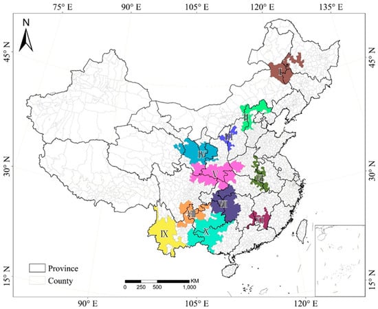
Figure 1.
Study area.
2.2. Data Sources
The NTL satellite data has the advantages of wide range, a long time period, unified standard, and having been obtained. It is an effective indicator of economic growth with a high correlation between NTL and economic indicators [,]. This study used the dataset of Chen et al. (2021) [], which adopt a cross-sensor calibration method. Firstly, the enhanced vegetation index adjusted to the NTL index was used to alleviate the saturation problem of DMSP/OLS data, and then the auto-encoder model with extended data generation was used. Finally, the extended NPP-VIIRS-like NTL data was generated with a spatial resolution of 15 arc seconds (≈500 m), showing good consistency at the pixel level and city level. The light intensity of each pixel in the dataset is represented by a number (DN) from 1 to 63 []. The dataset is available at https://doi.org/10.7910/DVN/YGIVCD (accessed on 14 April 2024) and has been widely used to study urbanization processes [,].
2.3. Overview of Methodology
The NTL data set and CDAs’ boundaries were used to extract all pixel DN in the CDAs from 2000 to 2020, set detection rules, compare the changes in the intensity and number of regional DN on a time scale, and, finally, classify counties (Figure 2a). This change detection was mainly carried out from two aspects. The first is object-oriented detection of regional NTL change (Figure 2b). The second is pixel-scale oriented (Figure 2c), quantizing its intensity and rate of change. Therefore, the spatial heterogeneity of NTL changes can be more accurately reflected.
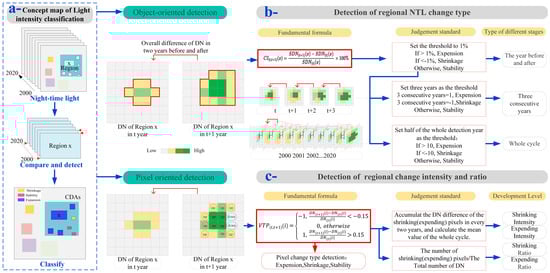
Figure 2.
Workflow of the methodology.
2.4. Identifying the Change Type of Counties in CDAs
Nighttime artificial lighting increases or decreases with the influence of population or economic activities, thus affecting the intensity of regional nighttime lighting [,]. From the perspective of spatial development, under the promotion of economic development, the expansion and intensity of regional construction land will inevitably lead to an increase in NTL, and the transformation of regional construction land use or a decrease in population and economic activities will inevitably lead to a decrease in NTL. To further judge the regional development situation. We quantified the variation of regional NTL by establishing rules and thresholds to distinguish the expansion, shrinkage, and stability of regional development. Based on previous research experience [,], we set three criteria: (1) The change of light in a certain region exceeds 1% compared with the previous year as the threshold. This is to determine whether the change in the following year is a trend of shrinkage, expansion, or stability. (2) Determine the type of phased regional change: if it is always shrinkage or expansion for three consecutive years. Then the period from the n year to the n+3 years in this region is a shrinking type or expanding type; otherwise, it is a stable type. To smooth the data, it is set as 2000–2002, 2002–2005, 2005–2008, 2008–2011, 2011–2014, 2014–2017, 2017–2020, a total of seven cycles, with 2000 to 2002 as the type of continuous change for two consecutive years as the standard for confirmation. (3) In the whole detection cycle, the type of regional change is determined. Based on (1), since 2000–2020 covers a total of 20 years, if more than half of those years (10 years) account for shrinking or expanding, this region is judged to be shrinking or expanding. Otherwise, it is judged as stable. The specific formula is as follows:
(1) Changes in light intensity over the previous two years:
where CI(t,t + 1)(x) is the ratio of change of light intensity in region x between t + 1 and t years, SDN(t)(x) and SDN(t + 1)(x) are the sums of DN of region x in t years and t + 1 years, respectively. TI(t,t + 1)(x) is the variation trend of light intensity in region x between t + 1 year and t year. If CI(t,t + 1)(x) is less than −1%, it is denoted as −1 for shrinkage, and if it is greater than 1% denoted as 1 for expansion. Otherwise, it is denoted as 0 for stability.
(2) Stage type of DN intensity change:
where TS(x) is a type of stage change. If TI(t,t + 1)(x) is −1 for three consecutive years, then TS(x) is a phased shrinkage, denoted as −1. If TI(t,t + 1)(x) is 1 for three consecutive years, then TS(x) is a phased expansion, denoted as 1. Otherwise, it is regarded as a stable type.
(3) Type of regional change throughout the cycle:
The period from 2000 to 2020 is 21 years in total and the comparison between the two years before and after produces 20-year changes. Based on the judgment of the light intensity of the two years before and after in region x, if more than half of the years in the 20-exhibit shrinkage, that is, the cumulative value is less than −10, it is considered that region x is in a shrinking development pattern throughout the cycle. If more than half of the 20 years are considered as expansion, the cumulative value is greater than 10, and region x is considered as having experienced expansion throughout the whole cycle. Otherwise, it is a stable type.
2.5. Measuring the Change Intensity and Ratio of Counties in CDAs
In order to further explore the dynamic characteristics of regional development, we quantified the variation of regional light intensity and the rate of light change. Firstly, the variation type of pixel scale is defined. Verify that the pixel is contracting, expanding, or stabilizing using the following formula:
Set 15% as the threshold []. If the DN of pixel i in the year (t + 1) is greater than 15% of the previous year (t), this pixel is an expanding pixel, denoted as 1; if the DN of pixel i in the year (t + 1) is less than −15% of the previous year (t), this pixel is shrinking, denoted as −1; otherwise, the pixel is considered stable, denoted as 0.
- (1)
- Average change intensity
Based on determining the type of changes in the pixel scale, calculate the total amount of changes with the pixel DN of the same type (shrinkage or expansion) in region x between t year and t + 1 year, and add up the annual changes from 2000 to 2020, and the change is 20 times. Therefore, the annual changes in the light intensity should be divided by 20.
ACI(x) is the average annual variation intensity of the light in region x, is the change of all (i) expanding/shrinking pixels in region x from one year to the next and then adds up the values of all the detection times, i.e., 2000–2001, 2001–2002, 2002–2003 … 2019–2020. All years are denoted as . Finally, divide by 20 years to get the average change intensity of the region x.
- (2)
- Average change ratio of regional DN
According to the judgment on the type of pixel change, we further calculate the number of changing pixels to represent the change ratio of regional DN.
ACR(x) Is the annual ratio of expansion or shrinkage of region x. NVTP(t,t + 1)(x) is the total number of pixels of region x that expand (or shrink) in the two years before and after t year and t + 1 year. NLP(t)(x) is the total number of pixels lit in region x in year t. Then calculate the proportion of expanding (or shrinking) pixels and add up the values for all the years of change. So, 2000–2001, 2001–2002, 2002–2003 … 2019–2020. All years are denoted as . Finally, divide by 20 years to get the average annual rate of change in light intensity.
2.6. Assessing the Risk of Returning to Poverty in CDAs
Through the above multi-period continuous threshold judgement method, we objectively classify counties as expanding, shrinking or stable. To further assess their risk of returning to poverty, we adopt a dual-tiered risk assessment framework from overall characteristics. Firstly, we use the NTL expansion area and luminance of each county during the study period to make judgements on the overall development pattern, and categorize them according to four patterns (Figure 3a): I. Both area and luminance are growing: this type has good economic development, and there is no risk of returning to poverty; II. The area is shrinking but luminance is increasing: this type is in the stage of smart growth, and there is no risk of returning to poverty; III. The area and luminance are showing a decreasing trend: this type shows obvious characteristics of economic decline, belonging to the apparent poverty return risk; IV. Area expansion but luminance decline: this type shows that economic development depends on area expansion, belonging to the hidden poverty return risk. By judging the risk patterns of the counties in the study area, we further use the time-series data of poverty assessment to classify the risk of returning to poverty. A county is considered to be of the type with a risk of returning to poverty if it appears to have a shrinkage mark (−1) after being marked as expanding in one period (+1) and fails to recover the expansion mark (+1) by the last period. In this case, we use the number of times a county has been marked with a shrinkage mark to classify the risk level, i.e., the more shrinkage, the higher the risk of returning to poverty.
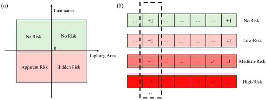
Figure 3.
(a) Risk patterns of overall characteristics, (b) Risk ranking based on time-series characteristics.
3. Results
3.1. Three Types of Spatiotemporal Distribution in CDAs
Using the NTL data from 2000 to 2020, this paper revealed the spatial development and change of counties in 11 CDAs (Figure 4). The 11 CDAs involved 532 counties and were divided into three categories: expansion, stability, and shrinkage. The number of each type was 345, 176, and 11, accounting for 64.85%, 33.08%, and 1.07%, respectively. In the expansion counties, the proportion of VI, XI, and VII was higher, ranging from 73.68% to 85.71%. However, the proportion of CDAs in China was less than 8.70%; the number of expansion counties of X, IV, and V was large, with 57, 47 and 47, accounting for 13.62–16.52%, and mainly concentrated in the Yunnan Province with 54 counties, Guizhou Province with 45 counties, and Gansu Province with 38 counties.
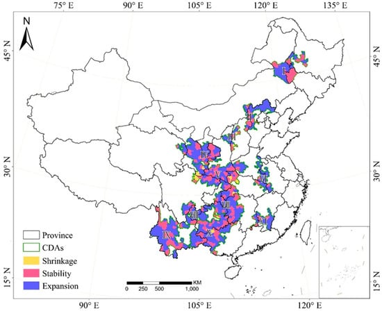
Figure 4.
Type of county change.
Shrinking counties were concentrated in V, VII, III, and X, with five, two, two, and two counties, respectively, and V was the largest, accounting for 45.45% of the shrinking counties in China. The distribution was mainly distributed in the provinces of Shanxi, Gansu, and Hubei.
A relatively large number of stable counties were concentrated in X, IV, V, and VII, with 23–30 counties, accounting for 32.86–35% of the region. It was worth noting that there were 20 stable counties in I, accounting for 54.55% of the region. In the province, the stable counties were mainly concentrated in Yunnan with 28, Guizhou with 21, and Gansu with 19 (Table 1).

Table 1.
The distribution of expanding, shrinking and stable counties.
3.2. Stage Characteristics of Space–Time Development of CDAs
Using a 4-year detection cycle, we identified the spatial development types of different counties in CDAs during 2000–2002, 2002–2005, 2005–2008, 2008–2011, 2011–2014, 2014–2017, and 2017–2020 (Figure 5a). The number of expanding counties in different periods changed greatly. The number of expansions was 283, 236, 203, 340, 255, 259, and 214, respectively. During the period from 2008 to 2011, expansion reached its peak (Figure 5b). From the perspective of the region, from 2008 to 2011, expansion counties were mainly concentrated in V, and X, with 53, 48, and 46 expansion counties, respectively. Shrinking counties: From 2000 to 2002, only 14 counties were shrinking. During 2002–2005, the number of shrinking counties was the largest, which was 235,225 from 2005 to 2008, mainly concentrated in IV, V and X. Since then, the number of shrinking counties has been reduced to 77 from 2008 to 2011 and gradually increased to 158 from 2017 to 2020. The number of stable counties increased from 235 in 2000 to 2002, to about 100 in each stage from 2005 to 2014, and about 160 from 2014 to 2020 (Figure 5c).
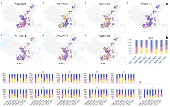
Figure 5.
Stage type of DN intensity change. (a) Stage change distribution, (b) the proportion of shrinking, expanding and stable counties at different stages stage change, (c) the proportion of shrinking, expanding and stable counties in different stages of each CDAs.
3.3. Change Intensity and Ratio of Counties in CDAs
Based on the natural breakpoint method, counties were categorized into five levels of intensity of change: low, relatively low, moderate, relatively high, and high (Figure 6). From 2000 to 2020, CDA expansion intensity comprised 109 low counties, 87 relatively low counties, 77 moderate counties, 52 relatively high counties, and 20 high counties, representing 31.59%, 25.22%, 22.32%, 15.07%, and 5.8% of all, respectively. Most counties were at the levels of expansion intensity with low or relatively low, and the counties with moderate, relatively high, and high levels of expansion were mainly concentrated in IV (24), VI (19), X (17), V (17), and VII (17).
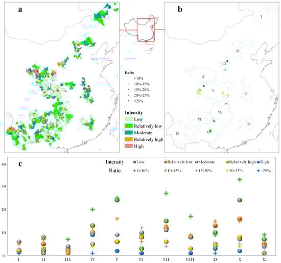
Figure 6.
Change intensity and ratio of counties. (a) Distribution of expansion intensity and ratio in expanding counties, (b) distribution of shrinking intensity and ratio in shrinking counties, (c) expansion intensity and ratio of expansion counties in different regions.
The expansion ratio in counties was divided into five levels: 0–10%, 10–15%, 15–20%, 20–25%, and >25%, accounting for 164 (47.54%), 105 (30.43%), 50 (14.50%), 19 (5.51%) and 7 (2.02%) of the counties, respectively. The counties with a change ratio greater than 15% were concentrated in IV (15), VI (15), IX (11), and X (9).
From the point of shrinkage, referring to the grading standard of expansion, the shrinking intensity can be divided into three levels, namely low, relatively low, and moderate. There were six counties in the low level, including V (4), VII (2), three counties in low level including X (2), III (1), and two counties in the moderate level, including V (1), III (1).
Referred to the standard of expansion ratio, the shrinking ratio of the county was 0–10% in III (1) and V (3), 10–15% in X (1), and VII (2), 15–20 in V (1), >25% in X (1), III (1), and V (1).
3.4. Poverty Return Risk Assessment in Counties
In this study, we analyzed 532 counties in the CDAs by the dual-tier poverty return risk assessment framework based on NTL data, from overall to the characteristics. The results show that there are 319 counties (59.96% of the total) with no risk of returning to poverty, i.e., the economic development has been growing during the study period, or there has been economic shrinkage but economic expansion has resumed. The total number of counties at risk of returning to poverty is 213. Among them, combining the time-series characteristics of each county, six counties were found to have never experienced economic expansion during the study period, indicating persistent poverty with no improvement. They are Susong County, Lixin County, Wufeng Tujia Autonomous County, Huayuan County, Gongshan Dulong-Nu Autonomous County, and Minhe Hui-Tu Autonomous County (blue labels in Figure 7). In terms of spatial distribution characteristics, the remaining five counties except Huayuan County are located at the outer edge of each CDA region. According to the identification of temporal characteristics, there are 147, 47, 11, 1, and 1 counties in order of low to high risk of returning to poverty. The counties with the lowest level of return to poverty risk (i.e., economic expansion followed by shrinkage but failed to expand again) are the most numerous, accounting for 27.63% of the total. In addition, in order to further reveal the hidden risk of poverty return, we screened out the fourth quadrant of 213 counties with poverty return risk, totaling 71 counties (purple labels in Figure 7).
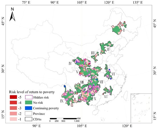
Figure 7.
County Return to Poverty Risk Assessment in CDAs.
4. Discussion
4.1. Spatiotemporal Characteristics of CDA Development and the Risk of Relapse into Poverty
Based on the research results, we further analyzed the characteristics of the spatiotemporal development of the poverty-stricken counties. First, on the whole, 98.93% of counties were spatially stable and expanding, which can support China’s poverty alleviation efforts. Expansion counties are concentrated in VI, XI, and VII. Mainly due to the geographical advantages of these three areas, the economic radiation of the urban agglomeration including the Yangtze River Delta, the middle reaches of the Yangtze River, the Pearl River Delta and the Chengdu–Chongqing urban agglomeration. A total of 1.07% of counties were shrinking. Through sorting out the basic information of these counties, it can be found that the factors affecting the shrinkage may be that the terrain of these areas is mainly hilly, high altitude, complex terrain, with serious soil erosion, and a poor ecological environment. Except for Tian’e County, the population has suffered a serious loss from 2000 to 2020, and the per capita income is significantly lower than the national average level. It shows that a fragile ecological environment and economic poverty coexist []. In addition, physical geographic factors also cause a series of problems, such as human resource cost, transportation, and backward informatization level, which affect regional development []. These regions are at risk of falling back into poverty.
Secondly, from the view of the phased development and change of poverty counties, the number of expanded counties in CDAs peaked during the period 2008–2011. This is mainly because, after the outbreak of the global financial crisis in 2008, the Chinese government launched ten measures to further expand domestic demand and promote steady and rapid economic growth, with an investment of about 4 trillion RMB by the end of 2010 []. It greatly promoted the construction of infrastructure and low-income housing projects, injecting dynamic factors into the expansion of poverty. In addition, the increasing level of urbanization in China, from 36.22% in 2000 to 60.34% in 2020, has led to the loss of cropland and environmental problems []. In particular, since 2011, China’s economic growth has slowed down [], and in recent years, the proportion of shrinkage has increased from 2017 to 2020.
Thirdly, in this study, we described the expansion intensity and ratio of expanding counties, and the shrinking intensity and ratio of shrinking counties. In fact, in the detection of regional change, the expansion and shrinking of the counties exist simultaneously. According to the ranking of expansion intensity, the four indicators of expansion intensity, shrinking intensity, expansion rate, and shrinking rate of the top 26 counties ranked at 5% are shown in Figure 8. There are 12 high-expansion counties in IV, mainly concentrated in Lanzhou City, including Chengguan District, Yongdeng County, Anning District, Xigu District, Qilihe District, Yuzhong County, and Gaolan County. Almost all of them were well-developed metropolitan areas or adjacent to big cities, with obvious regional advantages. At the same time, these counties also had a strongly shrinking intensity. It indicates that in the counties, the accumulative light intensity of pixels rather than a certain threshold value changes strongly, and the interior of these counties has strong vitality accompanied by expanding and shrinking in development. Therefore, most counties are expansionary with strong expanding and shrinking, and a few are stable, such as Chengguan District and Xigu District. The ratio of expansion and shrinkage is aimed at the number of pixels that reach a certain intensity of change in a region, which can be understood as the ratio of land expansion and shrinking from the perspective of geographical space. However, in all cases, the shrinking ratio is generally greater than the expansion ratio, indicating that the space where the light was weaker shrank substantially, while the space where the light was stronger expanded slightly. The space of CDAs was generally economical and characterized by intensive development. We should not only focus on the counties that show a contraction type. It is also necessary to pay attention to the counties with a large shrinkage ratio or contraction intensity, and there is also a potential trend of returning to poverty.
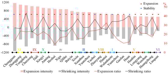
Figure 8.
Change characteristics of high expansion intensity.
4.2. A New Way to Measure the Development of Poverty Areas by Continuous Lighting Data
NTL data is widely used in regional development measurement research [,,]. NTL is good at spatially characterizing the heterogeneity of deprived areas. However, the expansion, shrinkage, and stabilization of the same area over time is ignored. Unlike previous studies on poverty measurement, we do not directly define the poverty criteria but use the nationally defined CDAs as the study area to identify the spatial and temporal changes of expansion and shrinkage based on NTL. It can reflect more accurately the internal heterogeneity of poverty areas. In the identification of different types of spatial–temporal changes in the counties of CDAs, the annual data of long time series are fully utilized, and the continuous and frequent shrinking and expansions are considered comprehensively, effectively reducing the uncertainty caused by accidental errors. After identifying the types of shrinkage, expansion, and stability in the CDAs, we focus on the changing intensity and ratio of the counties, which can reveal the reality of local shrinkage and expansion. The poverty areas are usually co-existing with this condition, and counties at risk of returning to poverty can be identified [].
In addition, NTL data also has the following advantages in the large-scale study of contiguously poor areas with special difficulties. First, it is easy to obtain and has a low cost. It has great application value and potential, especially in areas where reliable statistics may be lacking. Secondly, it helps in the understanding of the trajectory of the expansion and shrinkage of the poverty belt over a long period, which can reflect the effectiveness of the national poverty alleviation policy and the space–time response of the poverty belt to the social and economic changes. Thirdly, it contributes to horizontal comparative research in the global context and has great potential for cross-country comparison. This is especially true within countries and in regions where reliable statistics may be lacking, such as Africa []. Identifying the spatiotemporal development of poor areas based on NTL data can make up for the shortcomings of traditional data methods. It helps to monitor development changes and implement policies in poor areas from a global perspective.
4.3. Responses to Sustainable Development in CDAs
Based on our measurement and analysis of the development of poverty areas, some policy suggestions are put forward. In response to the problem of county shrinkage, a poverty alleviation and development model of “ecological migration-infrastructure integration-industrial development” should be established. This model aims to break the vicious cycle of poverty and ecological degradation, and specifically includes the following three steps:
1. Ecological migration. In areas with poor natural conditions and a bad ecological environment due to limited improvement in human resources, traditional development models are difficult to fundamentally solve the poverty problem. Therefore, gradual ecological migration measures should be taken to migrate residents from ecologically fragile and severely impoverished areas to new resettlement areas with better conditions, thereby laying the foundation for improving the living environment [,].
2. Infrastructure integration. In the new resettlement area, infrastructure construction must be promoted simultaneously, such as the construction of roads, water supply, power supply, communications and public service facilities. This can not only improve the basic living conditions of residents but also promote the efficient flow of resources in the region, and provide strong support for subsequent industrial development [].
3. Industrial development. Based on the phased development experience of CDAs, the state should further strengthen macro-policy guidance, such as supporting the tourism industry and increasing financial support, so as to give full play to the ecological, geographical and cultural advantages in the region [,]. At the same time, the government should strengthen its ties with developed regions and form a complete industrial and trade chain through counterpart support [,].
This model has been proven to be effective and feasible in poverty alleviation practices in the southern mountainous areas of Ningxia (study area IV, Liupan Mountains). In 1982, the Chinese government implemented the “Diaozhuang resettlement policy” (also called Diaozhuang immigration, an off-site resettlement policy) to solve the problem of food and clothing for farmers in the concentrated and contiguous poverty-stricken areas in southern Ningxia. For the farmers in the Xihaigu poverty areas of the original Liupan and Lipan mountain areas, the government implemented a development-oriented immigration poverty alleviation method through collective relocation of villages to the Pingchuan Yellow River Irrigation Area (including the Weining Irrigation Area and the Qingtongxia Irrigation Area) and the Yanghuang Irrigation Area. Meanwhile, the government provided special support funds to support rural infrastructure construction and agricultural industry development, and a total of 500,000 immigrants were relocate.
The implementation of this comprehensive policy not only improved the production and living conditions of residents but also alleviated the severe ecological pressure in the original Liupan mountain area, achieving the long-term and stable poverty alleviation goal. In addition, Qiandongnan, Guizhou Province and Enshi, Hubei Province have achieved the dual goals of protecting the ecology and alleviating poverty from this model.
It is worth noting that we still need to focus on counties where “expansion intensity is less than contraction intensity” and “both expansion and contraction intensity are low”. These areas lack development vitality and should adopt targeted industrial upgrading policies based on the actual difficulties of the local economy. Areas where the “expansion ratio is greater than contraction ratio” in counties also need attention. These areas are characterized by excessive reliance on land finance in the process of urbanization. This non-benign economic development structure is bound to have serious consequences. While exploring the transformation of industrial structure, we should strengthen the intensive use of construction land. In other words, we should revitalize the existing construction land and reduce the development of new construction land.
4.4. Limitations and Future Work
This study used existing NTL data to accurately portray the types of expansion/ shrinkage/stability, the dynamics of stage changes, and the changes in the intensity and ratio of expansion/shrinkage of CDAs in China, which objectively reveals the spatial and temporal dynamics of county development in the CDAs, and enriching poverty belt research results. However, there are still some problems. First, poverty is a condition of severe lack of basic human needs such as food, clothing, and shelter []. In China, the standard for poverty alleviation is that, with an annual per capita income of 4000 yuan (2020 standard), farmers have no shortage of food and clothing, and that they have medical, educational, and housing security. However, the development of CDAs is not only reflected in spatial changes, but also in economic and social welfare. The NTL data in this study reflect the spatial expansion/shrinkage characteristics of CDAs, but economic indicators, land use types, and other data need to be combined to further judge the degree of poverty alleviation development. Second, NTL data includes a large number of unlit areas as well as light-saturated county centers. The intensity of light at night is influenced by many different factors, such as changes in the number of vehicles equipped with car lighting, the existence of office buildings that operate at night, and the intensity of commercial activities at night. To obtain more accurate NTL data, it is necessary to conduct a more systematic correction analysis of the causes of light observed in different areas and different developmental contexts []. In the future, we will combine multi-source remote sensing data (such as POI) with socioeconomic and geographic indicators, such as GDP per capita, to capture the driving factors behind the expansion and contraction of poor areas. Meanwhile, we will deepen our understanding of regional poverty dynamics by expanding the scope of research to a wider provincial and national level. Capturing the spatiotemporal evolution of CDAs will enable the early identification of areas at risk of returning to poverty, while leveraging machine learning techniques will optimize threshold determination and improve dynamic monitoring for more adaptive poverty alleviation strategies.
5. Conclusions
Poverty is a dynamic phenomenon and process, with complexity, comprehensiveness, regionalism, and uncertainty. To accurately measure the development of CDAs, this study first proposed a classification method based on multi-period continuous threshold judgment using NTL data to identify the spatiotemporal changes of poverty-stricken areas in terms of contraction, expansion, and stability, and to measure the intensity and proportion of these changes. This method provides a new idea for the quantitative development and change of poverty-stricken areas with large scale and long time series, and fully considers spatial heterogeneity, critical periods, and the intensity and proportion of changes. Overall, the intensity and proportion of expansion and contraction are generally low, and counties with high expansion intensity are mainly distributed in regions IV, VI, X, V and VII. In addition, the risk of returning to poverty was assessed. The results showed that 40.04% of the counties were at risk of returning to poverty, but the overall risk was low. Future research should be based on multi-source remote sensing data (e.g., POI data) and introduce machine learning technology to optimize threshold judgment, improve the reliability of dynamic monitoring, and provide strong support for the formulation of more targeted and adaptive poverty alleviation strategies.
Author Contributions
Conceptualization, G.Z. and T.H.; methodology, J.W. and G.Z.; software, G.Z. and J.W.; validation, M.Z. and T.H.; formal analysis, G.Z.; investigation, J.W.; resources, J.W.; data curation, C.W. and T.H.; writing—original draft preparation, G.Z. and J.W.; writing—review and editing, G.Z. and C.W.; visualization, G.Z. and M.Z.; supervision, T.H.; project administration, C.W.; funding acquisition, T.H. All authors have read and agreed to the published version of the manuscript.
Funding
This research was funded by the Natural Science Foundation of Zhejiang Province, Approval No. Q22D018818 and the Zhejiang Provincial Philosophy and Social Science Planning Project, Approval No. 24JCXK04YB.
Data Availability Statement
The original contributions presented in this study are included in the article. Further inquiries can be directed to the corresponding author.
Conflicts of Interest
The authors declare no conflicts of interest.
References
- Liu, Y.; Zhou, Y.; Liu, J.L. Regional Differentiation Characteristics of Rural Poverty and Targeted Poverty Alleviation Strategy in China. Bull. Chin. Acad. Sci. 2016, 31, 269–278. [Google Scholar]
- Liu, Y.; Liu, J.; Zhou, Y. Spatio-Temporal Patterns of Rural Poverty in China and Targeted Poverty Alleviation Strategies. J. Rural. Stud. 2017, 52, 66–75. [Google Scholar] [CrossRef]
- Conceição, P. Human Development Report. In 2019: Beyond Income, beyond Averages, Beyond Today: Inequalities in Human Development in the 21st Century; United Nations Development Programme: New York, NY, USA, 2019. [Google Scholar]
- Yan, X.Y.; Qi, X.H. The Measurement Method and Evolution Mechanism of Poverty Dynamics. Acta Geogr. Sin. 2021, 76, 2425–2438. [Google Scholar]
- Zhu, X.; Peng, C. The Chinese Road: A Brilliant Chapter in the Cause of Human Anti-Poverty. In 40 Years of China’s War on Poverty; Springer: Berlin/Heidelberg, Germany, 2022; pp. 1–60. [Google Scholar]
- Pumariega, A.J.; Gogineni, R.R.; Benton, T. Poverty, Homelessness, Hunger in Children, and Adolescents: Psychosocial Perspectives. World Soc. Psychiatry 2022, 4, 54. [Google Scholar] [CrossRef]
- Ren, Q.; He, C.; Huang, Q. The Poverty Dynamics in the Agro-Pastoral Transitional Zone in Northern China: A Multiscale Perspective Based on the Poverty Gap Index. Resour. Sci. 2018, 40, 404–416. [Google Scholar]
- Rodgers, J.R.; Rodgers, J.L. Poverty Intensity in Australia. Aust. Econ. Rev. 2000, 33, 235–244. [Google Scholar] [CrossRef][Green Version]
- Orshansky, M. Children of the Poor. Soc. Secur. Bull. 1963, 26, 3. [Google Scholar]
- Zhang, Y.; Wan, G. The Impact of Growth and Inequality on Rural Poverty in China. J. Comp. Econ. 2006, 34, 694–712. [Google Scholar] [CrossRef]
- Bane, M.J.; Ellwood, D.T. Slipping into and out of Poverty: The Dynamics of Spells. J. Hum. Resour. 1986, 21, 1–23. [Google Scholar] [CrossRef]
- Jalan, J.; Ravallion, M. Transient Poverty in Postreform Rural China. J. Comp. Econ. 1998, 26, 338–357. [Google Scholar] [CrossRef]
- Johnson, D.S.; Levy, H.; Matsudaira, J.; Wolfe, B.L.; Ziliak, J.P. Measuring Poverty: Advances to the Supplemental Poverty Measure. ANNALS Am. Acad. Political Soc. Sci. 2024, 711, 20–37. [Google Scholar] [CrossRef]
- Zhang, F.; Liu, H.; Gu, W.; Zhang, J. Multidimensional Poverty and Types of Impoverished Counties in Gansu Province of China. Econ. Political Stud. 2022, 10, 105–125. [Google Scholar] [CrossRef]
- Wang, Y.; Chen, Y.; Chi, Y.; Zhao, W.; Hu, Z.; Duan, F. Village-Level Multidimensional Poverty Measurement in China: Where and How. J. Geogr. Sci. 2018, 28, 1444–1466. [Google Scholar] [CrossRef]
- Wang, M.; Wang, Y.; Teng, F.; Li, S.; Lin, Y.; Cai, H. China’s Poverty Assessment and Analysis under the Framework of the UN SDGs Based on Multisource Remote Sensing Data. Geo Spat. Inf. Sci. 2022, 27, 111–131. [Google Scholar]
- Li, G.; Chang, L.; Liu, X.; Su, S.; Cai, Z.; Huang, X.; Li, B. Monitoring the Spatiotemporal Dynamics of Poor Counties in China: Implications for Global Sustainable Development Goals. J. Clean. Prod. 2019, 227, 392–404. [Google Scholar] [CrossRef]
- Fan, Z.; Bai, X.; Zhao, N. Explicating the Responses of NDVI and GDP to the Poverty Alleviation Policy in Poverty Areas of China in the 21st Century. PLoS ONE 2022, 17, e0271983. [Google Scholar] [CrossRef]
- Hu, S.; Ge, Y.; Liu, M.; Ren, Z.; Zhang, X. Village-Level Poverty Identification Using Machine Learning, High-Resolution Images, and Geospatial Data. Int. J. Appl. Earth Obs. Geoinf. 2022, 107, 102694. [Google Scholar] [CrossRef]
- Jean, N.; Burke, M.; Xie, M.; Davis, W.M.; Lobell, D.B.; Ermon, S. Combining Satellite Imagery and Machine Learning to Predict Poverty. Science 2016, 353, 790–794. [Google Scholar] [CrossRef] [PubMed]
- Li, X.; Zhou, Y.; Zhao, M.; Zhao, X. A Harmonized Global Nighttime Light Dataset 1992–2018. Sci. Data 2020, 7, 168. [Google Scholar] [CrossRef]
- Ebener, S.; Murray, C.; Tandon, A.; Elvidge, C.C. From Wealth to Health: Modelling the Distribution of Income per Capita at the Sub-National Level Using Night-Time Light Imagery. Int. J. Health Geogr. 2005, 4, 5. [Google Scholar] [CrossRef]
- Xu, J.; Song, J.; Li, B.; Liu, D.; Cao, X. Combining Night Time Lights in Prediction of Poverty Incidence at the County Level. Appl. Geogr. 2021, 135, 102552. [Google Scholar] [CrossRef]
- Li, C.; Yang, W.; Tang, Q.; Tang, X.; Lei, J.; Wu, M.; Qiu, S. Detection of Multidimensional Poverty Using Luojia 1-01 Nighttime Light Imagery. J. Indian Soc. Remote Sens. 2020, 48, 963–977. [Google Scholar] [CrossRef]
- Su, Y.; Li, J.; Wang, D.; Yue, J.; Yan, X. Spatio-Temporal Synergy between Urban Built-Up Areas and Poverty Transformation in Tibet. Sustainability 2022, 14, 8773. [Google Scholar] [CrossRef]
- Yin, J.; Qiu, Y.; Zhang, B. Identification of Poverty Areas by Remote Sensing and Machine Learning: A Case Study in Guizhou, Southwest China. ISPRS Int. J. Geo Inf. 2020, 10, 11. [Google Scholar] [CrossRef]
- Yu, B.; Shi, K.; Hu, Y.; Huang, C.; Chen, Z.; Wu, J. Poverty Evaluation Using NPP-VIIRS Nighttime Light Composite Data at the County Level in China. IEEE J. Sel. Top. Appl. Earth Obs. Remote Sens. 2015, 8, 1217–1229. [Google Scholar] [CrossRef]
- Pan, J.; Hu, Y. Spatial Identification of Multi-Dimensional Poverty in Rural China: A Perspective of Nighttime-Light Remote Sensing Data. J. Indian Soc. Remote Sens. 2018, 46, 1093–1111. [Google Scholar] [CrossRef]
- Liu, T.; Yu, L.; Chen, X.; Li, X.; Du, Z.; Yan, Y.; Peng, D.; Gong, P. Utilizing Nighttime Light Datasets to Uncover the Spatial Patterns of County-Level Relative Poverty-Returning Risk in China and Its Alleviating Factors. J. Clean. Prod. 2024, 448, 141682. [Google Scholar] [CrossRef]
- Andreano, M.S.; Benedetti, R.; Piersimoni, F.; Savio, G. Mapping Poverty of Latin American and Caribbean Countries from Heaven Through Night-Light Satellite Images. Soc. Indic. Res. 2021, 156, 533–562. [Google Scholar] [CrossRef]
- Chen, W.; Feng, D.; Chu, X. Study of Poverty Alleviation Effects for Chinese Fourteen Contiguous Destitute Areas Based on Entropy Method. Int. J. Econ. Financ. 2015, 7, 89–98. [Google Scholar] [CrossRef]
- Hu, Y.; Yao, J. Illuminating Economic Growth. J. Econom. 2022, 228, 359–378. [Google Scholar] [CrossRef]
- Keola, S.; Andersson, M.; Hall, O. Monitoring Economic Development from Space: Using Nighttime Light and Land Cover Data to Measure Economic Growth. World Dev. 2015, 66, 322–334. [Google Scholar] [CrossRef]
- Chen, Z.; Yu, B.; Yang, C.; Zhou, Y.; Yao, S.; Qian, X.; Wang, C.; Wu, B.; Wu, J. An Extended Time Series (2000–2018) of Global NPP-VIIRS-like Nighttime Light Data from a Cross-Sensor Calibration. Earth Syst. Sci. Data 2021, 13, 889–906. [Google Scholar] [CrossRef]
- Yang, Y.; Wu, J.; Wang, Y.; Huang, Q.; He, C. Quantifying Spatiotemporal Patterns of Shrinking Cities in Urbanizing China: A Novel Approach Based on Time-Series Nighttime Light Data. Cities 2021, 118, 103346. [Google Scholar] [CrossRef]
- Chen, J.; Gao, M.; Cheng, S.; Hou, W.; Song, M.; Liu, X.; Liu, Y. Global 1 Km× 1 Km Gridded Revised Real Gross Domestic Product and Electricity Consumption during 1992–2019 Based on Calibrated Nighttime Light Data. Sci. Data 2022, 9, 202. [Google Scholar] [CrossRef]
- Wu, K.; You, K.; Ren, H.; Gan, L. The Impact of Industrial Agglomeration on Ecological Efficiency: An Empirical Analysis Based on 244 Chinese Cities. Environ. Impact Assess. Rev. 2022, 96, 106841. [Google Scholar] [CrossRef]
- Elvidge, C.D.; Hsu, F.-C.; Baugh, K.E.; Ghosh, T. National Trends in Satellite-Observed Lighting. Glob. Urban Monit. Assess. Through Earth Obs. 2014, 23, 97–118. [Google Scholar]
- Henderson, J.V.; Storeygard, A.; Weil, D.N. Measuring Economic Growth from Outer Space. Am. Econ. Rev. 2012, 102, 994–1028. [Google Scholar] [CrossRef]
- Hollander, J.B.; Németh, J. The Bounds of Smart Decline: A Foundational Theory for Planning Shrinking Cities. Hous. Policy Debate 2011, 21, 349–367. [Google Scholar] [CrossRef]
- Wu, K.; Li, Y. Research Progress of Urban Land Use and Its Ecosystem Services in the Context of Urban Shrinkage. J. Nat. Resour. 2019, 34, 1121. [Google Scholar] [CrossRef]
- Small, C.; Pozzi, F.; Elvidge, C.D. Spatial Analysis of Global Urban Extent from DMSP-OLS Night Lights. Remote Sens. Environ. 2005, 96, 277–291. [Google Scholar] [CrossRef]
- Cao, S.S.; Wang, Y.H.; Duan, F.Z.; Zhao, W.J.; Wang, Z.H.; Fang, N. Coupling between Ecological Vulnerability and Economic Poverty in Contiguous Destitute Areas, China: Empirical Analysis of 714 Poverty-Stricken Counties. Ying Yong Sheng Tai Xue Bao J. Appl. Ecol. 2016, 27, 2614–2622. [Google Scholar]
- Tian, Y.; Wang, Z.; Zhao, J.; Jiang, X.; Guo, R. A Geographical Analysis of the Poverty Causes in China’s Contiguous Destitute Areas. Sustainability 2018, 10, 1895. [Google Scholar] [CrossRef]
- Zheng, Y.; Chen, M. How Effective Will China’s Four Trillion Yuan Stimulus Plan Be? Univ. Nottm. China Policy Inst. Brief. Ser. 2009, 49, 28–37. [Google Scholar]
- Huang, Z.; Du, X.; Castillo, C.S.Z. How Does Urbanization Affect Farmland Protection? Evidence from China. Resour. Conserv. Recycl. 2019, 145, 139–147. [Google Scholar] [CrossRef]
- Glawe, L.; Wagner, H. China in the Middle-Income Trap? China Econ. Rev. 2020, 60, 101264. [Google Scholar] [CrossRef]
- Bennett, M.M.; Smith, L.C. Advances in Using Multitemporal Night-Time Lights Satellite Imagery to Detect, Estimate, and Monitor Socioeconomic Dynamics. Remote Sens. Environ. 2017, 192, 176–197. [Google Scholar] [CrossRef]
- Shen, Y. The Impact of Economic Growth and Inequality on Rural Poverty in China. J. Quant. Tech. Econ. 2012, 29, 19–34. [Google Scholar]
- Segers, T.; Devisch, O.; Herssens, J.; Vanrie, J. Conceptualizing Demographic Shrinkage in a Growing Region–Creating Opportunities for Spatial Practice. Landsc. Urban Plan. 2020, 195, 103711. [Google Scholar] [CrossRef]
- Feng, Q.; Zhou, Z.; Zhu, C.; Luo, W.; Zhang, L. Quantifying the Ecological Effectiveness of Poverty Alleviation Relocation in Karst Areas. Remote Sens. 2022, 14, 5920. [Google Scholar] [CrossRef]
- Ming, L.E.I.; Yuan, X.; Yao, X. Synthesize Dual Goals: A Study on China’s Ecological Poverty Alleviation System. J. Integr. Agric. 2021, 20, 1042–1059. [Google Scholar] [CrossRef]
- Zou, W.; Zhang, F.; Zhuang, Z.; Song, H. Transport Infrastructure, Growth, and Poverty Alleviation: Empirical Analysis of China. Ann. Econ. Financ. 2008, 9, 345–371. [Google Scholar]
- Cepparulo, A.; Cuestas, J.C.; Intartaglia, M. Financial Development, Institutions, and Poverty Alleviation: An Empirical Analysis. Appl. Econ. 2017, 49, 3611–3622. [Google Scholar] [CrossRef]
- Yang, X.; Zhou, X.; Cao, S.; Zhang, A. Preferences in Farmland Eco-Compensation Methods: A Case Study of Wuhan, China. Land 2021, 10, 1159. [Google Scholar] [CrossRef]
- Liu, P.; Qian, T.; Huang, X.; Dong, X. The Connotation, Realization Path and Measurement Method of Common Prosperity for All. Manag. World 2021, 37, 117–129. [Google Scholar]
Disclaimer/Publisher’s Note: The statements, opinions and data contained in all publications are solely those of the individual author(s) and contributor(s) and not of MDPI and/or the editor(s). MDPI and/or the editor(s) disclaim responsibility for any injury to people or property resulting from any ideas, methods, instructions or products referred to in the content. |
© 2025 by the authors. Licensee MDPI, Basel, Switzerland. This article is an open access article distributed under the terms and conditions of the Creative Commons Attribution (CC BY) license (https://creativecommons.org/licenses/by/4.0/).