
Multi-Source Attention U-Net: A Novel Deep Learning Framework for the Land Use and Soil Salinization Classification of Keriya Oasis in China with RADARSAT-2 and Landsat-8 Data

 , , and
Abstract
1. Introduction
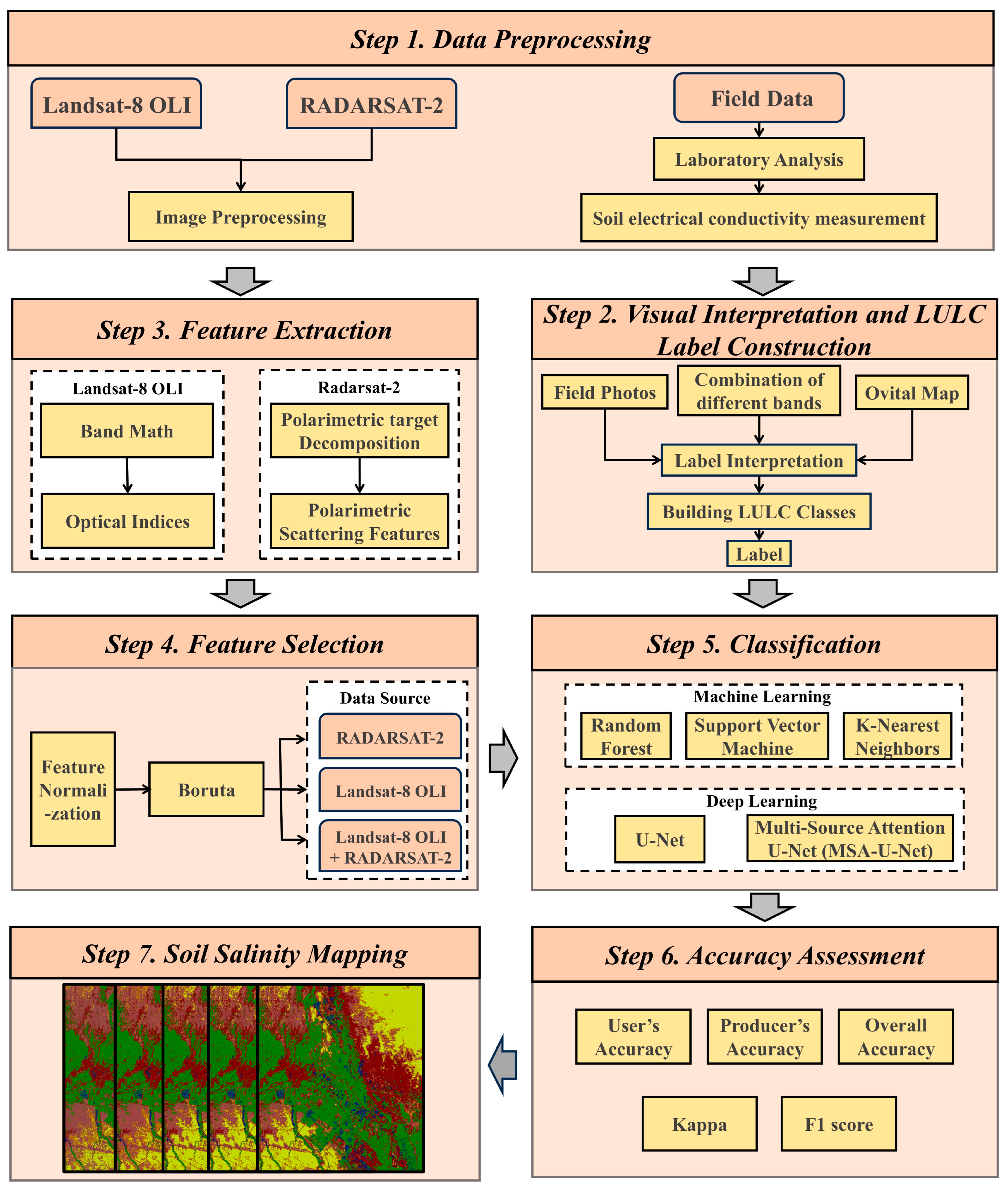
2. Materials
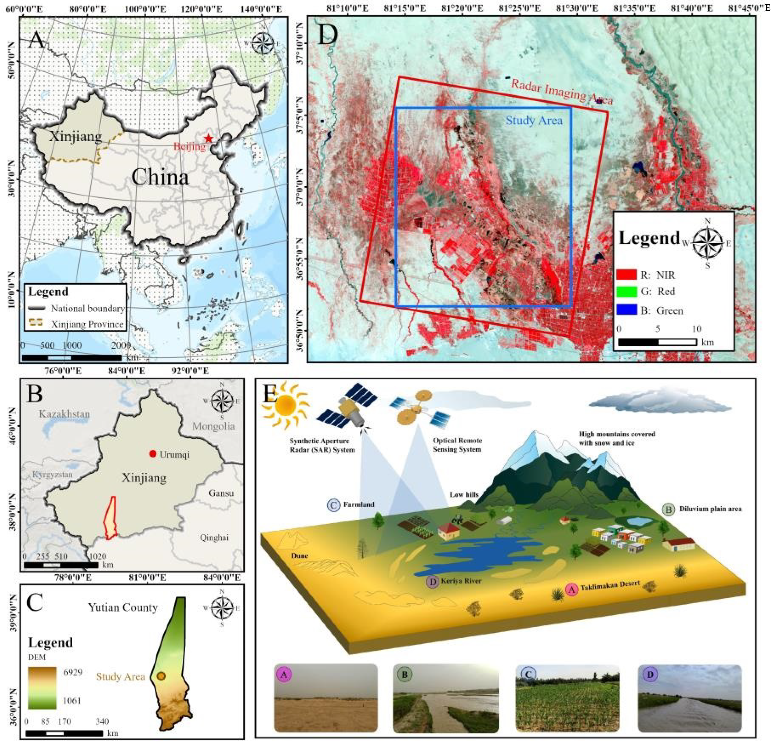
2.1. Study Site
2.2. Data Collection and Preprocessing
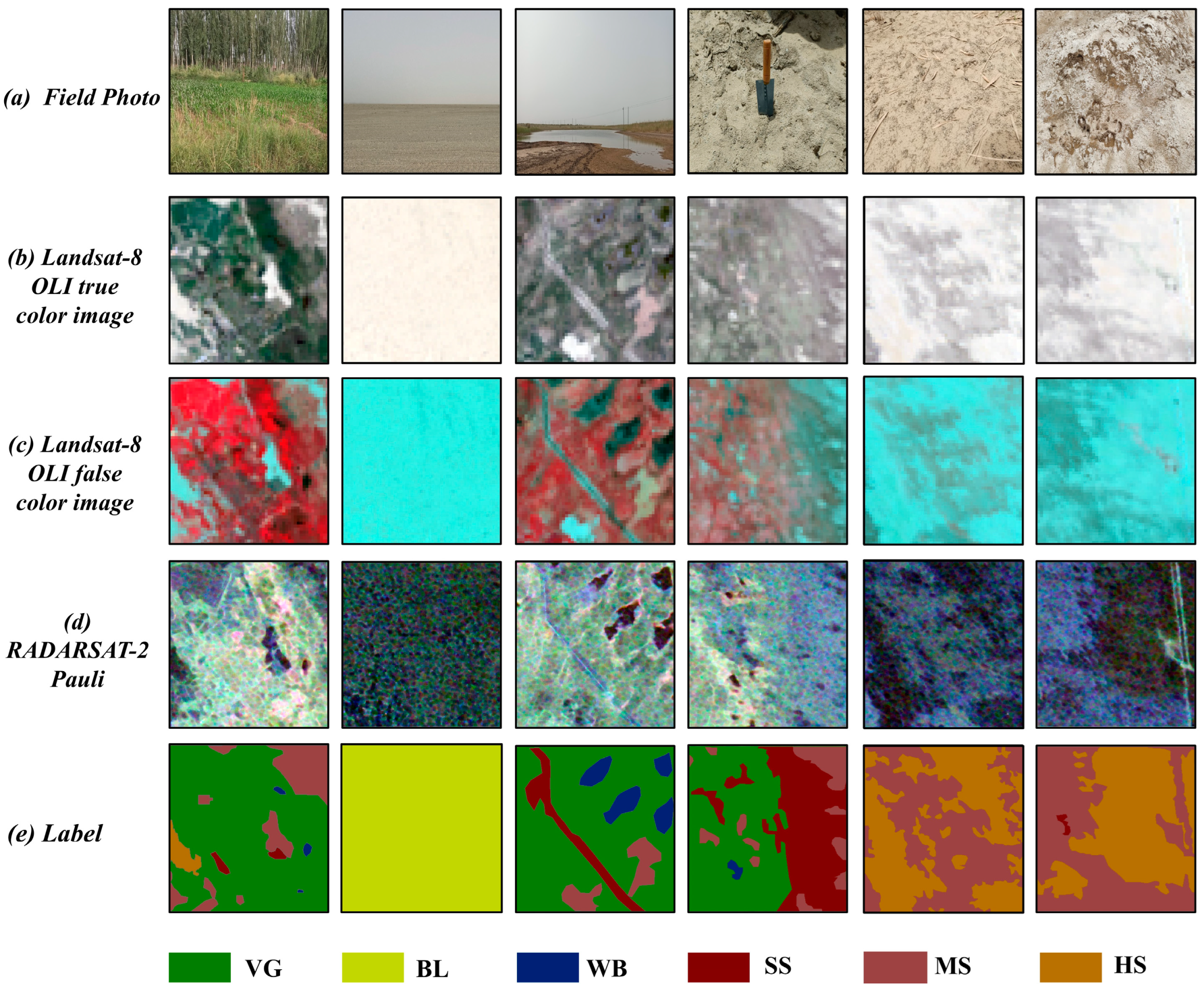
2.3. Field Data
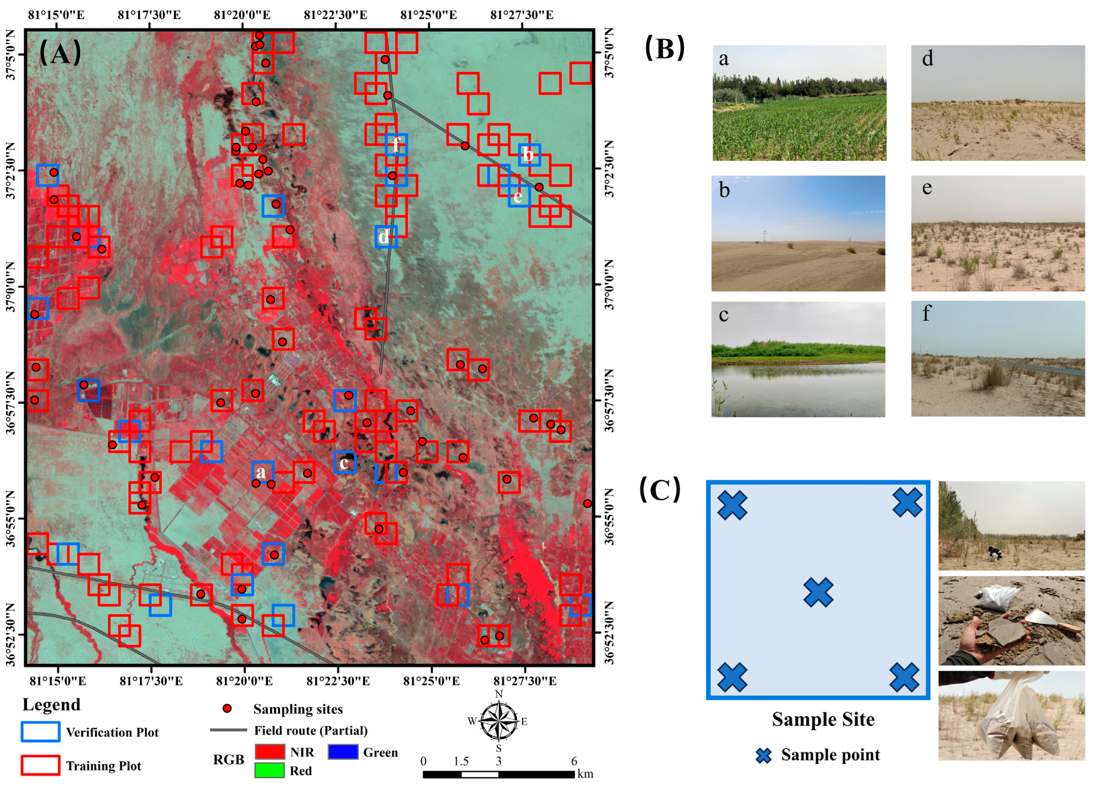
2.4. Collection of Training and Validation Data
3. Methods
3.1. Vegetation and Soil-Related Indices
3.2. Polarimetric Decomposition
3.3. Optimal Features Selection
3.4. Supervised Classification
3.4.1. Machine Learning Algorithms
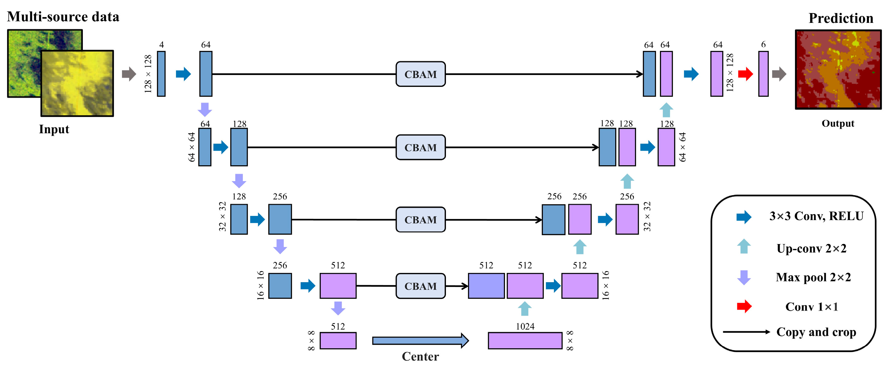
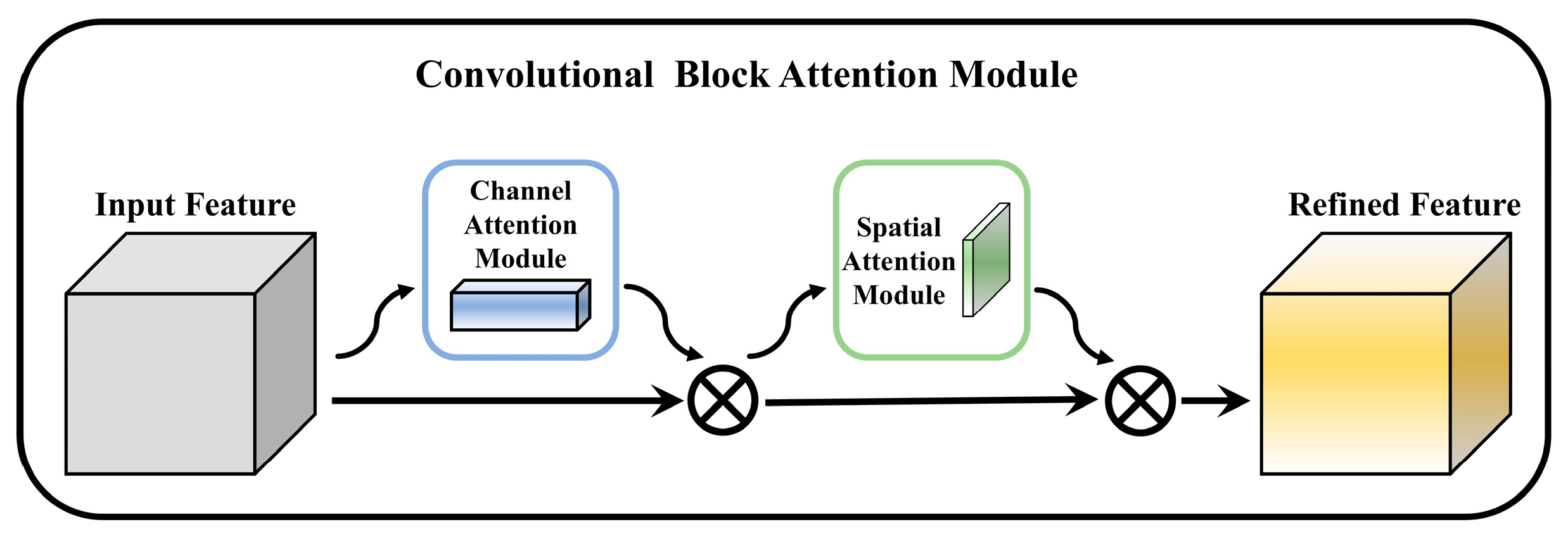
3.4.2. Deep Learning Algorithms
3.5. Model Evaluation Metrics
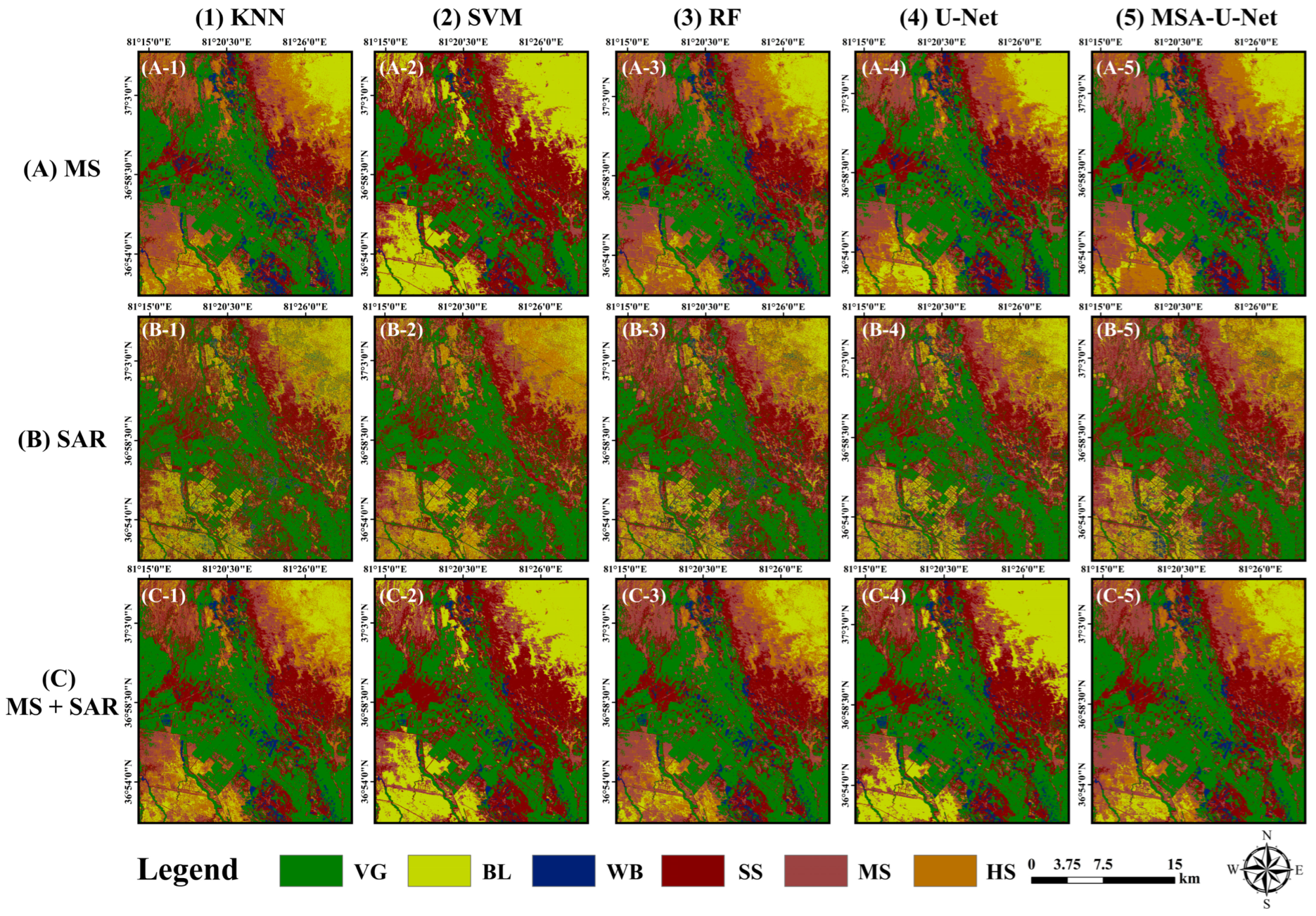
4. Results
4.1. Polarimetric Decomposition of RADARSAT-2 Data
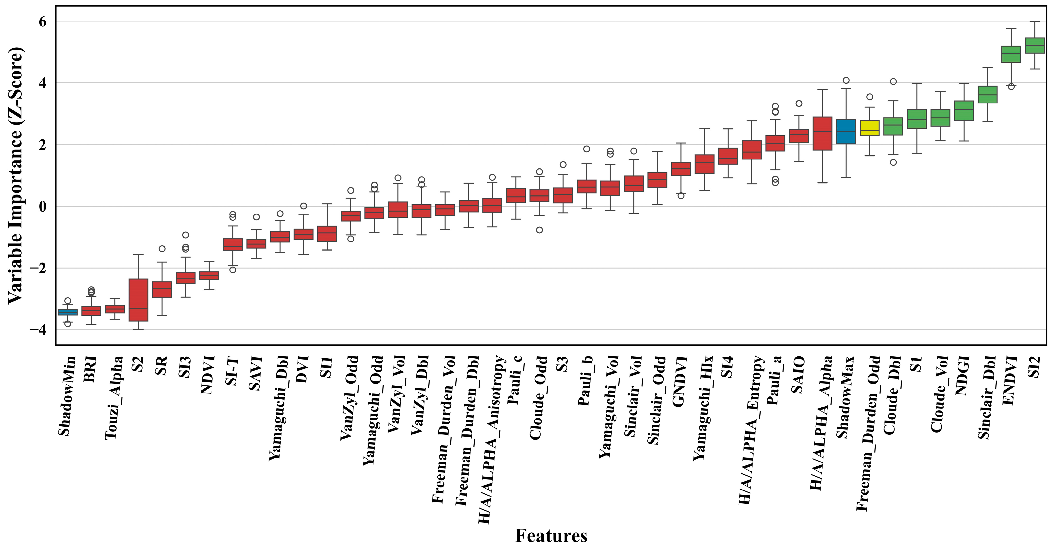
4.2. Feature Preprocessing and Selection of Optimal Feature Subset
4.3. Classification Results of MSA-U-Net
4.4. Comparison and Analysis of Classification Results Based on Multi-Sources Data
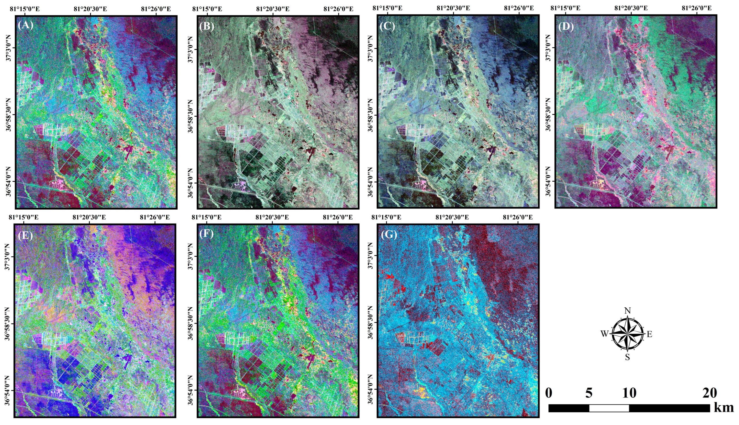
4.5. Characteristics of Spatial Distribution of Soil Salinity in Keriya Oasis
5. Discussion
5.1. Classification Performance Across Different Remote Sensing Data Sources
5.2. Comparison of MSA-U-Net with Traditional Machine Learning and Baseline Models
5.3. Impact of Attention Mechanisms on Skip Connections
5.4. Potential and Limitations
6. Conclusions
Author Contributions
Funding
Data Availability Statement
Acknowledgments
Conflicts of Interest
References
- Singh, A. Soil salinization management for sustainable development: A review. J. Environ. Manag. 2021, 277, 111383. [Google Scholar] [CrossRef] [PubMed]
- Singh, A. Soil salinization and waterlogging: A threat to environment and agricultural sustainability. Ecol. Indic. 2015, 57, 128–130. [Google Scholar] [CrossRef]
- Hafez, E.M.; Omara, A.E.D.; Alhumaydhi, F.A.; El-Esawi, M.A. Minimizing hazard impacts of soil salinity and water stress on wheat plants by soil application of vermicompost and biochar. Physiol. Plant. 2021, 172, 587–602. [Google Scholar] [CrossRef]
- Li, J.; Pu, L.; Han, M.; Zhu, M.; Zhang, R.; Xiang, Y. Soil salinization research in China: Advances and prospects. J. Geogr. Sci. 2014, 24, 943–960. [Google Scholar] [CrossRef]
- Barbouchi, M.; Abdelfattah, R.; Chokmani, K.; Aissa, N.B.; Lhissou, R.; El Harti, A. Soil salinity characterization using polarimetric InSAR coherence: Case studies in Tunisia and Morocco. IEEE J. Sel. Top. Appl. Earth Obs. Remote Sens. 2014, 8, 3823–3832. [Google Scholar] [CrossRef]
- Fathizad, H.; Ardakani, M.A.H.; Heung, B.; Sodaiezadeh, H.; Rahmani, A.; Fathabadi, A.; Scholten, T.; Taghizadeh-Mehrjardi, R. Spatio-temporal dynamic of soil quality in the central Iranian desert modeled with machine learning and digital soil assessment techniques. Ecol. Indic. 2020, 118, 106736. [Google Scholar] [CrossRef]
- Peng, J.; Biswas, A.; Jiang, Q.; Zhao, R.; Hu, J.; Hu, B.; Shi, Z. Estimating soil salinity from remote sensing and terrain data in southern Xinjiang Province, China. Geoderma 2019, 337, 1309–1319. [Google Scholar] [CrossRef]
- Ma, G.; Ding, J.; Han, L.; Zhang, Z.; Ran, S. Digital mapping of soil salinization based on Sentinel-1 and Sentinel-2 data combined with machine learning algorithms. Reg. Sustain. 2021, 2, 177–188. [Google Scholar] [CrossRef]
- Asfaw, E.; Suryabhagavan, K.; Argaw, M. Soil salinity modeling and mapping using remote sensing and GIS: The case of Wonji sugar cane irrigation farm, Ethiopia. J. Saudi Soc. Agric. Sci. 2018, 17, 250–258. [Google Scholar] [CrossRef]
- Yu, H.; Liu, M.; Du, B.; Wang, Z.; Hu, L.; Zhang, B. Mapping soil salinity/sodicity by using Landsat OLI imagery and PLSR algorithm over semiarid West Jilin Province, China. Sensors 2018, 18, 1048. [Google Scholar] [CrossRef]
- Metternicht, G.I.; Zinck, J. Remote sensing of soil salinity: Potentials and constraints. Remote Sens. Environ. 2003, 85, 1–20. [Google Scholar] [CrossRef]
- Ulaby, F.; Allen, C.; Eger Iii, G.; Kanemasu, E. Relating the microwave backscattering coefficient to leaf area index. Remote Sens. Environ. 1984, 14, 113–133. [Google Scholar] [CrossRef]
- Ulaby, F.T.; Moore, R.K.; Fung, A.K. Microwave Remote Sensing: Active and Passive. Volume 2-Radar Remote Sensing and Surface Scattering and Emission Theory; NASA: Washington, DC, USA, 1982. [Google Scholar]
- Rhoades, J.; Chanduvi, F.; Lesch, S. Soil Salinity Assessment: Methods and Interpretation of Electrical Conductivity Measurements; Food & Agriculture Organization: Rome, Italy, 1999. [Google Scholar]
- Grissa, M.; Abdelfattah, R.; Mercier, G.; Zribi, M.; Chahbi, A.; Lili-Chabaane, Z. Empirical model for soil salinity mapping from SAR data. In Proceedings of the 2011 IEEE International Geoscience and Remote Sensing Symposium, Vancouver, BC, Canada, 24–29 July 2011; pp. 1099–1102. [Google Scholar]
- Han, P.; Chen, Z.; Wan, Y.; Cheng, Z. PolSAR image classification based on optimal feature and convolution neural network. In Proceedings of the IGARSS 2020-2020 IEEE International Geoscience and Remote Sensing Symposium, Waikoloa, HI, USA, 26 September–2 October 2020; pp. 1735–1738. [Google Scholar]
- Qi, Z.; Yeh, A.G.-O.; Li, X.; Lin, Z. A novel algorithm for land use and land cover classification using RADARSAT-2 polarimetric SAR data. Remote Sens. Environ. 2012, 118, 21–39. [Google Scholar] [CrossRef]
- Zhang, Q.; Li, L.; Sun, R.; Zhu, D.; Zhang, C.; Chen, Q. Retrieval of the soil salinity from Sentinel-1 Dual-Polarized SAR data based on deep neural network regression. IEEE Geosci. Remote Sens. Lett. 2020, 19, 4006905. [Google Scholar] [CrossRef]
- Chen, S.-W.; Wang, X.-S.; Xiao, S.-P. Urban damage level mapping based on co-polarization coherence pattern using multitemporal polarimetric SAR data. IEEE J. Sel. Top. Appl. Earth Obs. Remote Sens. 2018, 11, 2657–2667. [Google Scholar] [CrossRef]
- Musthafa, M.; Khati, U.; Singh, G. Sensitivity of PolSAR decomposition to forest disturbance and regrowth dynamics in a managed forest. Adv. Space Res. 2020, 66, 1863–1875. [Google Scholar] [CrossRef]
- Wei, Q.; Nurmemet, I.; Gao, M.; Xie, B. Inversion of soil salinity using multisource remote sensing data and particle swarm machine learning models in Keriya Oasis, northwestern China. Remote Sens. 2022, 14, 512. [Google Scholar] [CrossRef]
- Zhu, X.X.; Tuia, D.; Mou, L.; Xia, G.-S.; Zhang, L.; Xu, F.; Fraundorfer, F. Deep learning in remote sensing: A comprehensive review and list of resources. IEEE Geosci. Remote Sens. Mag. 2017, 5, 8–36. [Google Scholar] [CrossRef]
- Kussul, N.; Lavreniuk, M.; Skakun, S.; Shelestov, A. Deep learning classification of land cover and crop types using remote sensing data. IEEE Geosci. Remote Sens. Lett. 2017, 14, 778–782. [Google Scholar] [CrossRef]
- Garg, R.; Kumar, A.; Bansal, N.; Prateek, M.; Kumar, S. Semantic segmentation of PolSAR image data using advanced deep learning model. Sci. Rep. 2021, 11, 15365. [Google Scholar] [CrossRef]
- Gao, J.; Deng, B.; Qin, Y.; Wang, H.; Li, X. Enhanced radar imaging using a complex-valued convolutional neural network. IEEE Geosci. Remote Sens. Lett. 2018, 16, 35–39. [Google Scholar] [CrossRef]
- Fu, G.; Liu, C.; Zhou, R.; Sun, T.; Zhang, Q. Classification for high resolution remote sensing imagery using a fully convolutional network. Remote Sens. 2017, 9, 498. [Google Scholar] [CrossRef]
- Garcia-Garcia, A.; Orts-Escolano, S.; Oprea, S.; Villena-Martinez, V.; Garcia-Rodriguez, J. A review on deep learning techniques applied to semantic segmentation. arXiv 2017, arXiv:1704.06857. [Google Scholar] [CrossRef]
- Ronneberger, O.; Fischer, P.; Brox, T. U-net: Convolutional networks for biomedical image segmentation. In Proceedings of the Medical Image Computing and Computer-Assisted Intervention–MICCAI 2015: 18th International Conference, Munich, Germany, 5–9 October 2015; proceedings, part III 18. 2015; pp. 234–241. [Google Scholar]
- Han, Z.; Dian, Y.; Xia, H.; Zhou, J.; Jian, Y.; Yao, C.; Wang, X.; Li, Y. Comparing fully deep convolutional neural networks for land cover classification with high-spatial-resolution Gaofen-2 images. ISPRS Int. J. Geo-Inf. 2020, 9, 478. [Google Scholar] [CrossRef]
- Akca, S.; Gungor, O. Semantic segmentation of soil salinity using in-situ EC measurements and deep learning based U-NET architecture. Catena 2022, 218, 106529. [Google Scholar] [CrossRef]
- Solórzano, J.V.; Mas, J.F.; Gao, Y.; Gallardo-Cruz, J.A. Land use land cover classification with U-net: Advantages of combining sentinel-1 and sentinel-2 imagery. Remote Sens. 2021, 13, 3600. [Google Scholar] [CrossRef]
- Clark, A.; Phinn, S.; Scarth, P. Optimised U-Net for land use–land cover classification using aerial photography. PFG–J. Photogramm. Remote Sens. Geoinf. Sci. 2023, 91, 125–147. [Google Scholar] [CrossRef]
- Zhao, J.; Nurmemet, I.; Muhetaer, N.; Xiao, S.; Abulaiti, A. Monitoring Soil Salinity Using Machine Learning and the Polarimetric Scattering Features of PALSAR-2 Data. Sustainability 2023, 15, 7452. [Google Scholar] [CrossRef]
- Wang, J.; Li, W.; Gao, Y.; Zhang, M.; Tao, R.; Du, Q. Hyperspectral and SAR Image Classification via Multiscale Interactive Fusion Network. IEEE Trans. Neural Netw. Learn. Syst. 2023, 34, 10823–10837. [Google Scholar] [CrossRef]
- Chen, B.; Huang, B.; Xu, B. Multi-source remotely sensed data fusion for improving land cover classification. ISPRS J. Photogramm. Remote Sens. 2017, 124, 27–39. [Google Scholar] [CrossRef]
- Hughes, L.H.; Marcos, D.; Lobry, S.; Tuia, D.; Schmitt, M. A deep learning framework for matching of SAR and optical imagery. ISPRS J. Photogramm. Remote Sens. 2020, 169, 166–179. [Google Scholar] [CrossRef]
- Sommervold, O.; Gazzea, M.; Arghandeh, R. A survey on SAR and optical satellite image registration. Remote Sens. 2023, 15, 850. [Google Scholar] [CrossRef]
- Kulkarni, S.C.; Rege, P.P. Pixel level fusion techniques for SAR and optical images: A review. Inf. Fusion 2020, 59, 13–29. [Google Scholar] [CrossRef]
- Chen, C.; Yuan, X.; Gan, S.; Kang, X.; Luo, W.; Li, R.; Bi, R.; Gao, S. A new strategy based on multi-source remote sensing data for improving the accuracy of land use/cover change classification. Sci. Rep. 2024, 14, 26855. [Google Scholar] [CrossRef] [PubMed]
- Zhang, G.; Roslan, S.N.A.B.; Wang, C.; Quan, L. Research on land cover classification of multi-source remote sensing data based on improved U-net network. Sci. Rep. 2023, 13, 16275. [Google Scholar] [CrossRef] [PubMed]
- Woo, S.; Park, J.; Lee, J.-Y.; Kweon, I.S. Cbam: Convolutional block attention module. In Proceedings of the European Conference on Computer Vision (ECCV), Munich, Germany, 8–14 September 2018; pp. 3–19. [Google Scholar]
- Haut, J.M.; Fernandez-Beltran, R.; Paoletti, M.E.; Plaza, J.; Plaza, A. Remote sensing image superresolution using deep residual channel attention. IEEE Trans. Geosci. Remote Sens. 2019, 57, 9277–9289. [Google Scholar] [CrossRef]
- Yu, X.; Qian, Y.; Geng, Z.; Huang, X.; Wang, Q.; Zhu, D. EMC²A-Net: An Efficient Multibranch Cross-Channel Attention Network for SAR Target Classification. IEEE Trans. Geosci. Remote Sens. 2023, 61, 5210314. [Google Scholar] [CrossRef]
- Nurmemet, I.; Sagan, V.; Ding, J.-L.; Halik, Ü.; Abliz, A.; Yakup, Z. A WFS-SVM model for soil salinity mapping in Keriya Oasis, Northwestern China using polarimetric decomposition and fully PolSAR data. Remote Sens. 2018, 10, 598. [Google Scholar] [CrossRef]
- Du, M.; Li, L.; Luo, G.; Dong, K.; Shi, Q. Effects of climate and land use change on agricultural water consumption in Yutian Oasis. Bull. Soil Water Conserv. 2020, 40, 103–109. [Google Scholar]
- Muhetaer, N.; Nurmemet, I.; Abulaiti, A.; Xiao, S.; Zhao, J. An efficient approach for inverting the soil salinity in Keriya Oasis, northwestern China, based on the optical-radar feature-space model. Sensors 2022, 22, 7226. [Google Scholar] [CrossRef]
- Yang, S.; Yang, T. Exploration of the dynamic water resource carrying capacity of the Keriya River Basin on the southern margin of the Taklimakan Desert, China. Reg. Sustain. 2021, 2, 73–82. [Google Scholar] [CrossRef]
- Mamat, Z.; Yimit, H.; Lv, Y. Spatial distributing pattern of salinized soils and their salinity in typical area of Yutian Oasis. Chin. J. Soil Sci. 2013, 44, 1314–1320. [Google Scholar]
- Zhang, B.; Perrie, W.; He, Y. Validation of RADARSAT-2 fully polarimetric SAR measurements of ocean surface waves. J. Geophys. Res. Oceans 2010, 115. [Google Scholar] [CrossRef]
- Jiang, Y.; Ding, F.; Ma, R.; Li, X.; Xu, X. Atmospheric correction algorithms comparison for Lake Water based on Landsat8 images. In Proceedings of the 2018 Fifth International Workshop on Earth Observation and Remote Sensing Applications (EORSA), Xi’an, China, 18–20 June 2018; pp. 1–5. [Google Scholar]
- Faizan, M. Radarsat-2 Data Processing Using SNAP Software; Anna University: Chennai, India, 2020. [Google Scholar]
- Liu, X.; Chi, C. Relationships of electrical conductivity between 1:5 soil/water extracts and saturation paste extracts of salt-affected soils in southern Xinjiang. Jiangsu Agric. Sci. 2015, 43, 289–291. [Google Scholar] [CrossRef]
- Tian Yong, J.Z.; Chen, L.; Xi, H.; Zhang, B.; Gan, K. Characteristics of soil water and salt spatial differentiation along the Yellow River section of Ulan Buh Desert and its causes. J. Desert Res. 2024, 44, 247–258. [Google Scholar] [CrossRef]
- Gao, Z.; Li, X.; Zuo, L.; Zou, B.; Wang, B.; Wang, W.J. Unveiling soil salinity patterns in soda saline-alkali regions using Sentinel-2 and SDGSAT-1 thermal infrared data. Remote Sens. Environ. 2025, 322, 114708. [Google Scholar] [CrossRef]
- Han, L.; Ding, J.; Zhang, J.; Chen, P.; Wang, J.; Wang, Y.; Wang, J.; Ge, X.; Zhang, Z. Precipitation events determine the spatiotemporal distribution of playa surface salinity in arid regions: Evidence from satellite data fused via the enhanced spatial and temporal adaptive reflectance fusion model. Catena 2021, 206, 105546. [Google Scholar] [CrossRef]
- Abuelgasim, A.; Ammad, R. Mapping soil salinity in arid and semi-arid regions using Landsat 8 OLI satellite data. RSASE 2019, 13, 415–425. [Google Scholar] [CrossRef]
- Abulaiti, A.; Nurmemet, I.; Muhetaer, N.; Xiao, S.; Zhao, J. Monitoring of soil salinization in the Keriya Oasis based on deep learning with PALSAR-2 and Landsat-8 datasets. Sustainability 2022, 14, 2666. [Google Scholar] [CrossRef]
- Brady, N.C.; Weil, R.R.; Weil, R.R. The Nature and Properties of Soils; Prentice Hall: Upper Saddle River, NJ, USA, 2008; Volume 13. [Google Scholar]
- Chi, M.; Feng, R.; Bruzzone, L. Classification of hyperspectral remote-sensing data with primal SVM for small-sized training dataset problem. Adv. Space Res. 2008, 41, 1793–1799. [Google Scholar] [CrossRef]
- Sawangarreerak, S.; Thanathamathee, P. Random forest with sampling techniques for handling imbalanced prediction of university student depression. Information 2020, 11, 519. [Google Scholar] [CrossRef]
- Goetz, A.F.; Rock, B.N.; Rowan, L.C. Remote sensing for exploration; an overview. Econ. Geol. 1983, 78, 573–590. [Google Scholar] [CrossRef]
- Li, X.; Zhang, F.; Wang, Z. Present situation and development trend of remote sensing monitoring model for soil salinization. Remote Sens. Nat. Resour. 2022, 34, 11–21. [Google Scholar] [CrossRef]
- Fernandez-Buces, N.; Siebe, C.; Cram, S.; Palacio, J. Mapping soil salinity using a combined spectral response index for bare soil and vegetation: A case study in the former lake Texcoco, Mexico. J. Arid Environ. 2006, 65, 644–667. [Google Scholar] [CrossRef]
- Peñuelas, J.; Llusià, J. Effects of carbon dioxide, water supply, and seasonality on terpene content and emission by Rosmarinus officinalis. J. Chem. Ecol. 1997, 23, 979–993. [Google Scholar] [CrossRef]
- Allbed, A.; Kumar, L.; Aldakheel, Y.Y. Assessing soil salinity using soil salinity and vegetation indices derived from IKONOS high-spatial resolution imageries: Applications in a date palm dominated region. Geoderma 2014, 230, 1–8. [Google Scholar] [CrossRef]
- Zhang, Z.; Ding, J.; Zhu, C.; Wang, J.; Ma, G.; Ge, X.; Li, Z.; Han, L. Strategies for the efficient estimation of soil organic matter in salt-affected soils through Vis-NIR spectroscopy: Optimal band combination algorithm and spectral degradation. Geoderma 2021, 382, 114729. [Google Scholar] [CrossRef]
- Alavipanah, S.K.; Damavandi, A.A.; Mirzaei, S.; Rezaei, A.; Hamzeh, S.; Matinfar, H.R.; Teimouri, H.; Javadzarrin, I. Remote sensing application in evaluation of soil characteristics in desert areas. Nat. Environ. Change 2016, 2, 1–24. [Google Scholar]
- Chen, J.M. Evaluation of vegetation indices and a modified simple ratio for boreal applications. CaJRS 1996, 22, 229–242. [Google Scholar] [CrossRef]
- DeFries, R.S.; Townshend, J. NDVI-derived land cover classifications at a global scale. Int. J. Remote Sens. 1994, 15, 3567–3586. [Google Scholar] [CrossRef]
- Huete, A.R. A soil-adjusted vegetation index (SAVI). Remote Sens. Environ. 1988, 25, 295–309. [Google Scholar] [CrossRef]
- Gitelson, A.A.; Kaufman, Y.J.; Merzlyak, M.N. Use of a green channel in remote sensing of global vegetation from EOS-MODIS. Remote Sens. Environ. 1996, 58, 289–298. [Google Scholar] [CrossRef]
- Jordan, C.F. Derivation of leaf-area index from quality of light on the forest floor. Ecology 1969, 50, 663–666. [Google Scholar] [CrossRef]
- Nedkov, R. Normalized Differential Greenness Index for vegetation dynamics assessment. Comptes Rendus L’academie Bulg. Sci. 2017, 70, 1143–1146. [Google Scholar]
- Hongyan, C.; Gengxing, Z.; Jingchun, C.; Ruiyan, W.; Mingxiu, G. Remote sensing inversion of saline soil salinity based on modified vegetation index in estuary area of Yellow River. Trans. Chin. Soc. Agric. Eng. 2015, 31, 107–114. [Google Scholar] [CrossRef]
- Tripathi, N.; Rai, B.K.; Dwivedi, P. Spatial modeling of soil alkalinity in GIS environment using IRS data. In Proceedings of the Proceedings of the 18th Asian Conference on Remote Sensing, Kuala Lumpur, Malaysia, 20–24 October 1997; pp. 81–86. [Google Scholar]
- Khan, N.M.; Rastoskuev, V.V.; Sato, Y.; Shiozawa, S. Assessment of hydrosaline land degradation by using a simple approach of remote sensing indicators. Agric. Water Manag. 2005, 77, 96–109. [Google Scholar] [CrossRef]
- Nicolas, H.; Walter, C. Detecting salinity hazards within a semiarid context by means of combining soil and remote-sensing data. Geoderma 2006, 134, 217–230. [Google Scholar] [CrossRef]
- Abbas, A.; Khan, S. Using remote sensing techniques for appraisal of irrigated soil salinity. In Proceedings of the International Congress on Modelling and Simulation (MODSIM), Christchurch, New Zealand, 10–13 December 2007; pp. 2632–2638. [Google Scholar]
- Taghizadeh-Mehrjardi, R.; Minasny, B.; Sarmadian, F.; Malone, B. Digital mapping of soil salinity in Ardakan region, central Iran. Geoderma 2014, 213, 15–28. [Google Scholar] [CrossRef]
- Huynen, J.R. Phenomenological Theory of Radar Targets; Academic Press: Cambridge, MA, USA, 1970. [Google Scholar]
- Trudel, M.; Magagi, R.; Granberg, H.B. Application of target decomposition theorems over snow-covered forested areas. IEEE Trans. Geosci. Remote Sens. 2009, 47, 508–512. [Google Scholar] [CrossRef]
- Mishra, P.; Singh, D.; Yamaguchi, Y. Land cover classification of PALSAR images by knowledge based decision tree classifier and supervised classifiers based on SAR observables. Prog. Electromagn. Res. B 2011, 30, 47–70. [Google Scholar] [CrossRef]
- An, W.; Cui, Y.; Yang, J. Three-component model-based decomposition for polarimetric SAR data. IEEE Trans. Geosci. Remote Sens. 2010, 48, 2732–2739. [Google Scholar] [CrossRef]
- Cloude, S.R.; Pottier, E. A review of target decomposition theorems in radar polarimetry. IEEE Trans. Geosci. Remote Sens. 1996, 34, 498–518. [Google Scholar] [CrossRef]
- Freeman, A.; Durden, S.L. A three-component scattering model for polarimetric SAR data. IEEE Trans. Geosci. Remote Sens. 1998, 36, 963–973. [Google Scholar] [CrossRef]
- Yamaguchi, Y.; Moriyama, T.; Ishido, M.; Yamada, H. Four-component scattering model for polarimetric SAR image decomposition. IEEE Trans. Geosci. Remote Sens. 2005, 43, 1699–1706. [Google Scholar] [CrossRef]
- Cloude, S.R. Target decomposition theorems in radar scattering. ElL 1985, 21, 22–24. [Google Scholar] [CrossRef]
- van Zyl, J.J. Application of Cloude’s target decomposition theorem to polarimetric imaging radar data. In Proceedings of the Radar Polarimetry; SPIE: St. Bellingham, WA, USA, 1993; pp. 184–191. [Google Scholar]
- Cloude, S.R.; Pottier, E. An entropy based classification scheme for land applications of polarimetric SAR. IEEE Trans. Geosci. Remote Sens. 1997, 35, 68–78. [Google Scholar] [CrossRef]
- Touzi, R. Target scattering decomposition in terms of roll-invariant target parameters. IEEE Trans. Geosci. Remote Sens. 2006, 45, 73–84. [Google Scholar] [CrossRef]
- Kursa, M.B.; Jankowski, A.; Rudnicki, W.R. Boruta—A system for feature selection. Fundam. Informaticae 2010, 101, 271–285. [Google Scholar] [CrossRef]
- Xiao, S.; Nurmemet, I.; Zhao, J. Soil salinity estimation based on machine learning using the GF-3 radar and Landsat-8 data in the Keriya Oasis, Southern Xinjiang, China. Plant Soil. 2024, 498, 451–469. [Google Scholar] [CrossRef]
- Cover, T.; Hart, P. Nearest neighbor pattern classification. ITIT 1967, 13, 21–27. [Google Scholar] [CrossRef]
- Yu, Z. Research on Remote Sensing Image Terrain Classification Algorithm Based on Improved KNN. In Proceedings of the 2020 IEEE 3rd International Conference on Information Systems and Computer Aided Education (ICISCAE), Dalian, China, 27–29 September 2020; pp. 569–573. [Google Scholar]
- Samaniego, L.; Bárdossy, A.; Schulz, K. Supervised classification of remotely sensed imagery using a modified k-NN technique. IEEE Trans. Geosci. Remote Sens. 2008, 46, 2112–2125. [Google Scholar] [CrossRef]
- Hechenbichler, K.; Schliep, K. Weighted k-Nearest-Neighbor Techniques and Ordinal Classification; Ludwig Maximilian University of Munich: Munich, Germany, 2004. [Google Scholar] [CrossRef]
- Haq, Y.U.; Shahbaz, M.; Asif, S.; Ouahada, K.; Hamam, H. Identification of Soil Types and Salinity Using MODIS Terra Data and Machine Learning Techniques in Multiple Regions of Pakistan. Sensors 2023, 23, 8121. [Google Scholar] [CrossRef] [PubMed]
- Vermeulen, D.; Van Niekerk, A. Machine learning performance for predicting soil salinity using different combinations of geomorphometric covariates. Geoderma 2017, 299, 1–12. [Google Scholar] [CrossRef]
- Vapnik, V. The Nature of Statistical Learning Theory; Springer Science & Business Media: Berlin/Heidelberg, Germany, 2013. [Google Scholar]
- Mountrakis, G.; Im, J.; Ogole, C. Support vector machines in remote sensing: A review. ISPRS J. Photogramm. Remote Sens. 2011, 66, 247–259. [Google Scholar] [CrossRef]
- Mantero, P.; Moser, G.; Serpico, S.B. Partially supervised classification of remote sensing images through SVM-based probability density estimation. IEEE Trans. Geosci. Remote Sens. 2005, 43, 559–570. [Google Scholar] [CrossRef]
- Wang, J.; Peng, J.; Li, H.; Yin, C.; Liu, W.; Wang, T.; Zhang, H. Soil salinity mapping using machine learning algorithms with the Sentinel-2 MSI in arid areas, China. Remote Sens. 2021, 13, 305. [Google Scholar] [CrossRef]
- Breiman, L. Random forests. Mach. Learn. 2001, 45, 5–32. [Google Scholar] [CrossRef]
- Wang, F.; Yang, S.; Wei, Y.; Shi, Q.; Ding, J. Characterizing soil salinity at multiple depth using electromagnetic induction and remote sensing data with random forests: A case study in Tarim River Basin of southern Xinjiang, China. Sci. Total Environ. 2021, 754, 142030. [Google Scholar] [CrossRef]
- Fathizad, H.; Ardakani, M.A.H.; Sodaiezadeh, H.; Kerry, R.; Taghizadeh-Mehrjardi, R. Investigation of the spatial and temporal variation of soil salinity using random forests in the central desert of Iran. Geoderma 2020, 365, 114233. [Google Scholar] [CrossRef]
- Wang, F.; Shi, Z.; Biswas, A.; Yang, S.; Ding, J. Multi-algorithm comparison for predicting soil salinity. Geoderma 2020, 365, 114211. [Google Scholar] [CrossRef]
- Gislason, P.O.; Benediktsson, J.A.; Sveinsson, J.R. Random forest classification of multisource remote sensing and geographic data. In Proceedings of the IGARSS 2004. 2004 IEEE International Geoscience and Remote Sensing Symposium, Anchorage, AK, USA, 20–24 September 2004; pp. 1049–1052. [Google Scholar]
- Sheykhmousa, M.; Mahdianpari, M.; Ghanbari, H.; Mohammadimanesh, F.; Ghamisi, P.; Homayouni, S. Support vector machine versus random forest for remote sensing image classification: A meta-analysis and systematic review. IEEE J. Sel. Top. Appl. Earth Obs. Remote Sens. 2020, 13, 6308–6325. [Google Scholar] [CrossRef]
- Ronneberger, O.; Fischer, P.; Brox, T.; Navab, N.; Hornegger, J.; Wells, W.M.; Frangi, A.F. Medical image computing and computer-assisted intervention–MICCAI 2015. Lect. Notes Comput. Sci. 2015, 9351, 234–241. [Google Scholar]
- Nair, V.; Hinton, G.E. Rectified linear units improve restricted boltzmann machines. In Proceedings of the 27th International Conference on Machine Learning (ICML-10), Haifa, Israel, 21–24 June 2010; pp. 807–814. [Google Scholar]
- Kinga, D.; Adam, J.B. A method for stochastic optimization. In Proceedings of the International Conference on Learning Representations (ICLR), San Diego, CA, USA, 7–9 May 2015; p. 6. [Google Scholar]
- Congalton, R.G. A review of assessing the accuracy of classifications of remotely sensed data. Remote Sens. Environ. 1991, 37, 35–46. [Google Scholar] [CrossRef]
- Dehaan, R.; Taylor, G. Field-derived spectra of salinized soils and vegetation as indicators of irrigation-induced soil salinization. Remote Sens. Environ. 2002, 80, 406–417. [Google Scholar] [CrossRef]
- Ravi, K.P.; Periasamy, S. Systematic discrimination of irrigation and upheaval associated salinity using multitemporal SAR data. Sci. Total Environ. 2021, 790, 148148. [Google Scholar] [CrossRef]
- Periasamy, S.; Ravi, K.P.; Tansey, K. Identification of saline landscapes from an integrated SVM approach from a novel 3-D classification schema using Sentinel-1 dual-polarized SAR data. Remote Sens. Environ. 2022, 279, 113144. [Google Scholar] [CrossRef]
- Garajeh, M.K.; Malakyar, F.; Weng, Q.; Feizizadeh, B.; Blaschke, T.; Lakes, T. An automated deep learning convolutional neural network algorithm applied for soil salinity distribution mapping in Lake Urmia, Iran. Sci. Total Environ. 2021, 778, 146253. [Google Scholar] [CrossRef]
- Liu, C.; Sun, Y.; Xu, Y.; Sun, Z.; Zhang, X.; Lei, L.; Kuang, G. A review of optical and SAR image deep feature fusion in semantic segmentation. IEEE J. Sel. Top. Appl. Earth Obs. Remote Sens. 2024, 17, 12910–12930. [Google Scholar] [CrossRef]
- Muhammad, W.; Aramvith, S.; Onoye, T. SENext: Squeeze-and-ExcitationNext for single image super-resolution. IEEE Access 2023, 11, 45989–46003. [Google Scholar] [CrossRef]
- Fu, J.; Liu, J.; Tian, H.; Li, Y.; Bao, Y.; Fang, Z.; Lu, H. Dual attention network for scene segmentation. In Proceedings of the IEEE/CVF Conference on Computer Vision and Pattern Recognition, Long Beach, CA, USA, 15–20 June 2019; pp. 3146–3154. [Google Scholar]
- Aleissaee, A.A.; Kumar, A.; Anwer, R.M.; Khan, S.; Cholakkal, H.; Xia, G.-S.; Khan, F.S. Transformers in remote sensing: A survey. Remote Sens. 2023, 15, 1860. [Google Scholar] [CrossRef]
- Liu, X.; Zhang, C.; Zhang, L. Vision mamba: A comprehensive survey and taxonomy. arXiv 2024, arXiv:2405.04404. [Google Scholar] [CrossRef]
- Zhang, H.; Wan, L.; Wang, T.; Lin, Y.; Lin, H.; Zheng, Z. Impervious surface estimation from optical and polarimetric SAR data using small-patched deep convolutional networks: A comparative study. IEEE J. Sel. Top. Appl. Earth Obs. Remote Sens. 2019, 12, 2374–2387. [Google Scholar] [CrossRef]
- Kang, W.; Xiang, Y.; Wang, F.; You, H. CFNet: A cross fusion network for joint land cover classification using optical and SAR images. IEEE J. Sel. Top. Appl. Earth Obs. Remote Sens. 2022, 15, 1562–1574. [Google Scholar] [CrossRef]

| Remote Sensing | RADARSAT-2 | Landsat-8 |
|---|---|---|
| Map Projection | WGS84 (DD) | UTM |
| Sensor | C-band synthetic aperture radar | Operational Land Imager |
| Data Observation Date | 6 May 2022 | 18 May 2022 |
| Product Type | SLC | L2SP |
| Nominal Resolution | 5.5 m 4.8 m | 30 m |
| Incident angle/Orbit Inclination Angle | 42.1° | 98.2° |
| Revisit Time | 24 d | 16 d |
| Orbit Type | Sun Synchronous Orbit | Sun Synchronous Orbit |
| Satellite Attitude | 798 km | 705 km |
| Band Number | --- | 11 |
| Polarizations | HH, HV, VV, VH | --- |
| Symbol | Class | Characteristics | Typical Filed Photos |
|---|---|---|---|
| WB | Water Body | Salt lakes, rivers and tributaries, swamps, ponds, and reservoirs. | 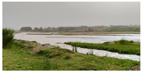 |
| VG | Vegetation | Grassland, farmland, red willow, populus euphratica, reed, camel thorn, and dried riverbed. | 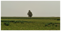 |
| BL | Barren Land | Gobi, desert, wasteland, and bare land. | 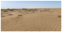 |
| SS | Slightly Salinized soil | EC value 2–4 (dS/m), covered by a thin salt crust (0–2 cm), and the vegetation coverage is around 30%. | 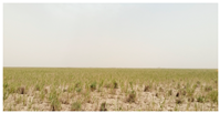 |
| MS | Moderately Salinized soil | EC value of 4–8 (dS/m), with a salt crust thickness of 1 to 4 cm and a vegetation coverage of around 5 to 15%. |  |
| HS | Highly Salinized soil | EC value of 8–16 (dS/m), covered by a thin salt crust (4–10 cm), and the vegetation coverage is less than 5%. | 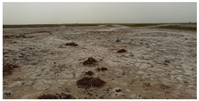 |
| Class | Abbreviation | Training (70%) | Validation (30%) | ||
|---|---|---|---|---|---|
| Plots | Pixels | Plots | Pixels | ||
| Vegetation | VG | 42 | 4290 | 18 | 1810 |
| Barren Land | BL | 20 | 2877 | 9 | 1090 |
| Water Body | WB | 18 | 1576 | 8 | 1004 |
| Slightly Salinized soil | SS | 35 | 3542 | 15 | 1406 |
| Moderately Salinized soil | MS | 32 | 3195 | 14 | 1367 |
| Highly Salinized soil | HS | 33 | 3433 | 16 | 1743 |
| Total | - | 180 | 17,913 | 70 | 8420 |
| Category | Index | Calculation Formula | Reference |
|---|---|---|---|
| Vegetation Indices | Simple Ratio Vegetation Index (SR) | [68] | |
| Normalized Difference Vegetation Index (NDVI) | [69] | ||
| Soil Adjusted Vegetation Index (SAVI) | [70] | ||
| Green Normalized Difference Vegetation Index (GNDVI) | [71] | ||
| Differential Vegetation Index (DVI) | [72] | ||
| Normalized Difference Green Index (NDGI) | [73] | ||
| Enhanced Normalized Vegetation Index (ENDVI) | [74] | ||
| Soil-related Indices | Salinity Index (SI-T) | [75] | |
| Salinity Index (SI1) | [76] | ||
| Salinity Index (SI2) | [77] | ||
| Salinity Index (SI3) | [77] | ||
| Salinity Index (SI4) | [78] | ||
| Salinity Index (S1) | [77] | ||
| Salinity Index (S2) | [78] | ||
| Salinity Index (S3) | [78] | ||
| Salinity Ratio Index (SAIO) | [79] | ||
| Brightness Index (BRI) | [79] |
| Polarization Decomposition | Number of Features | Polarimetric Scattering Features |
|---|---|---|
| Pauli | 3 | Pauli_a/Pauli_b/Pauli_c |
| Cloude | 3 | Cloude_Dbl/Cloude_Odd/Cloude_Vol |
| H/A/Alpha | 3 | Alpha/Anisotropy/Entropy |
| VanZyl | 3 | VanZyl_Vol/VanZyl_Odd/VanZyl_Dbl |
| Freeman-Durden | 3 | Freeman_Durden_Dbl/Freeman_Durden_Odd/Freeman_Durden_Vol |
| Sinclair | 3 | Sinclair_Dbl/Sinclair_Vol/Sinclair_Surf |
| Touzi | 4 | Alpha/Psi*/Phi*/Tau* |
| Yamaguchi | 4 | Yamaguchi_Dbl/Yamaguchi_Odd/Yamaguchi_Vol/Yamaguchi_Hlx |
| KNN | SVM | RF | U-Net | MSA-U-Net | ||||||
|---|---|---|---|---|---|---|---|---|---|---|
| PA (%) | UA (%) | PA (%) | UA (%) | PA (%) | UA (%) | PA (%) | UA (%) | PA (%) | UA (%) | |
| WB | 90.32 | 88.89 | 87.90 | 91.60 | 90.32 | 87.50 | 87.10 | 85.71 | 88.33 | 85.48 |
| VG | 83.45 | 81.12 | 82.01 | 87.69 | 84.17 | 82.98 | 79.86 | 82.84 | 82.14 | 82.14 |
| BL | 72.43 | 79.76 | 97.30 | 63.83 | 72.43 | 81.71 | 97.30 | 75.63 | 92.18 | 89.19 |
| SS | 66.67 | 62.18 | 51.11 | 93.88 | 70.37 | 75.25 | 72.22 | 92.20 | 86.96 | 88.89 |
| MS | 61.04 | 61.04 | 57.14 | 65.67 | 79.22 | 63.21 | 68.18 | 82.68 | 81.99 | 85.71 |
| HS | 80.38 | 81.41 | 83.03 | 78.61 | 85.44 | 91.22 | 92.41 | 83.91 | 91.67 | 90.51 |
| OA (%) | 74.79 | 77.66 | 79.10 | 82.98 | 87.34 | |||||
| Kappa | 0.69 | 0.73 | 0.74 | 0.76 | 0.84 | |||||
| Data Source | Classification Methods | OA (%) | Kappa | F1 Score |
|---|---|---|---|---|
| Landsat-8 OLI (MS) | KNN | 76.38 | 0.71 | 0.77 |
| SVM | 73.08 | 0.67 | 0.72 | |
| RF | 77.36 | 0.75 | 0.80 | |
| U-Net | 79.15 | 0.74 | 0.79 | |
| MSA-U-Net | 79.57 | 0.75 | 0.80 | |
| RADARSAT-2 (SAR) | KNN | 51.38 | 0.41 | 0.51 |
| SVM | 52.98 | 0.43 | 0.51 | |
| RF | 55.64 | 0.46 | 0.56 | |
| U-Net | 50.85 | 0.40 | 0.50 | |
| MSA-U-Net | 51.49 | 0.41 | 0.51 | |
| Landsat-8 + RADARSAT-2 (MS + SAR) | KNN | 74.79 | 0.69 | 0.75 |
| SVM | 77.66 | 0.73 | 0.77 | |
| RF | 79.10 | 0.75 | 0.80 | |
| U-Net | 82.98 | 0.79 | 0.82 | |
| MSA-U-Net | 87.34 | 0.84 | 0.87 |
| Models | U-Net | U-Net-SAM | U-Net-CAM | MSA-U-Net | ||||
|---|---|---|---|---|---|---|---|---|
| Classes | PA (%) | UA (%) | PA (%) | UA (%) | PA (%) | UA (%) | PA (%) | UA (%) |
| VG | 79.86 | 82.84 | 84.89 | 80.82 | 83.45 | 82.27 | 82.73 | 82.14 |
| BL | 97.30 | 75.63 | 92.43 | 89.53 | 88.65 | 90.61 | 89.19 | 92.18 |
| WT | 87.10 | 85.71 | 84.68 | 88.98 | 84.68 | 89.74 | 85.48 | 88.33 |
| SS | 92.41 | 83.91 | 90.51 | 91.08 | 91.14 | 90.57 | 90.51 | 91.67 |
| MS | 68.18 | 82.68 | 83.12 | 79.01 | 84.42 | 80.75 | 85.71 | 81.99 |
| HS | 72.22 | 92.20 | 83.89 | 90.96 | 84.44 | 83.98 | 88.89 | 86.96 |
| OA (%) | 82.98 | 86.81 | 86.28 | 87.34 | ||||
| Kappa coefficient | 0.79 | 0.84 | 0.83 | 0.84 | ||||
| F1 score | 0.82 | 0.86 | 0.86 | 0.87 | ||||
Disclaimer/Publisher’s Note: The statements, opinions and data contained in all publications are solely those of the individual author(s) and contributor(s) and not of MDPI and/or the editor(s). MDPI and/or the editor(s) disclaim responsibility for any injury to people or property resulting from any ideas, methods, instructions or products referred to in the content. |
© 2025 by the authors. Licensee MDPI, Basel, Switzerland. This article is an open access article distributed under the terms and conditions of the Creative Commons Attribution (CC BY) license (https://creativecommons.org/licenses/by/4.0/).
Share and Cite
Xiang, Y.; Nurmemet, I.; Lv, X.; Yu, X.; Gu, A.; Aihaiti, A.; Li, S. Multi-Source Attention U-Net: A Novel Deep Learning Framework for the Land Use and Soil Salinization Classification of Keriya Oasis in China with RADARSAT-2 and Landsat-8 Data. Land 2025, 14, 649. https://doi.org/10.3390/land14030649
Xiang Y, Nurmemet I, Lv X, Yu X, Gu A, Aihaiti A, Li S. Multi-Source Attention U-Net: A Novel Deep Learning Framework for the Land Use and Soil Salinization Classification of Keriya Oasis in China with RADARSAT-2 and Landsat-8 Data. Land. 2025; 14(3):649. https://doi.org/10.3390/land14030649
Chicago/Turabian StyleXiang, Yang, Ilyas Nurmemet, Xiaobo Lv, Xinru Yu, Aoxiang Gu, Aihepa Aihaiti, and Shiqin Li. 2025. "Multi-Source Attention U-Net: A Novel Deep Learning Framework for the Land Use and Soil Salinization Classification of Keriya Oasis in China with RADARSAT-2 and Landsat-8 Data" Land 14, no. 3: 649. https://doi.org/10.3390/land14030649
APA StyleXiang, Y., Nurmemet, I., Lv, X., Yu, X., Gu, A., Aihaiti, A., & Li, S. (2025). Multi-Source Attention U-Net: A Novel Deep Learning Framework for the Land Use and Soil Salinization Classification of Keriya Oasis in China with RADARSAT-2 and Landsat-8 Data. Land, 14(3), 649. https://doi.org/10.3390/land14030649