Article

Spatiotemporal Patterns and Determinants of Cropland Abandonment in Mountainous Regions of China: A Case Study of Sichuan Province

1
School of Geography and Ocean Science, Nanjing University, Nanjing 210023, China
2
Key Laboratory of Coastal Zone Exploitation and Protection, Ministry of Natural Resources, Nanjing 210023, China
3
Key Laboratory of Carbon Neutrality and Territory Optimization, Ministry of Natural Resources, Nanjing 210023, China
4
Key Laboratory of Land Resources Evaluation and Monitoring in Southwest China, Ministry of Education, Sichuan Normal University, Chengdu 610066, China
5
Institute of Geography and Resources Science, Sichuan Normal University, Chengdu 610101, China
*
Author to whom correspondence should be addressed.
Land 2025, 14(3), 647; https://doi.org/10.3390/land14030647
Submission received: 23 February 2025 / Revised: 13 March 2025 / Accepted: 17 March 2025 / Published: 18 March 2025
(This article belongs to the Section Land Socio-Economic and Political Issues)

Abstract

:
Cropland abandonment (CA) is an increasingly severe global issue, with significant implications for achieving the Sustainable Development Goal of Zero Hunger. In China, widespread CA is particularly evident in remote mountainous regions. However, the rugged terrain and highly fragmented cropland pose significant challenges in mapping abandoned cropland with high precision using remote sensing technology. Moreover, CA is the result of multi-level factors, yet previous studies have primarily analyzed its driving factors from a single level, leading to a lack of comprehensive understanding of the underlying mechanisms. We took Sichuan Province, located in the mountainous regions of Western China, as a case study, utilizing satellite-derived high-precision CA maps to reveal the spatiotemporal patterns of CA. Additionally, we employed hierarchical linear model to explore the determinants of CA and their interactions at both county and municipal levels. The results indicate that the CA rate decreased continuously from 6.75% in 2019 to 4.47% in 2023, with abandoned cropland exhibiting significant spatial clustering. High-value clusters were predominantly concentrated in the western mountainous areas, and hotspots of CA exhibited a general migration trend from the northeast to the southwest. Furthermore, we found that CA is influenced by multi-level factors, with 61% and 39% of the variance in CA being explained at the county and municipal levels, respectively. The agglomeration index of cropland (AI) is a key determinant at the county level, with the Digital Elevation Model (DEM) and the distance to roads also playing significant roles. At the municipal level, urbanization rate and the proportion of non-agricultural employment (PNAE) are dominant factors, and an increase in PNAE weakens the negative impact of AI on CA rates. To curb CA in mountainous areas, we recommend implementing land consolidation projects, improving rural land transfer markets, and strengthening legal mechanisms to combat CA. Our study has broad application prospects, providing critical support for assessing the ecological and environmental consequences of CA and exploring the potential of reutilizing abandoned cropland for food production, bioenergy, and carbon sequestration.

1. Introduction

Eradicating hunger, achieving food security, improving nutrition, and promoting sustainable agriculture are critical goals for global sustainable development [1]. However, the latest assessment data reveal that hunger and food insecurity remain pervasive. In 2023, approximately 733 million people worldwide faced hunger, and 2.33 billion experienced moderate to severe food insecurity. All regions urgently require sustained and coordinated actions to enhance agricultural productivity and sustainability by 2030 [2]. Cropland is the foundation for food production and an essential resource for sustainable agricultural development. However, cropland abandonment (CA) has been observed in many regions globally [3,4,5,6], with the scale reaching hundreds of millions of hectares [7]. CA refers to the discontinuation of agricultural activities, leading to unmanaged, uncultivated, or underutilized cropland [8,9]. Although there are contrasting views on the ecological and environmental impacts of CA, ranging from positive to negative [10,11,12], there is a consensus that CA will result in reduced grain production and exacerbate food insecurity [13,14,15]. Reclaiming new cropland to expand cultivation areas poses a threat to natural habitats and biodiversity [16,17,18] and is widely regarded as an undesirable option [19]. In contrast, abandoned cropland, with its historical cultivation foundation and conditions, offers a critical pathway for addressing future food security challenges through reclamation [7,20]. Moreover, reforesting or planting perennial grasses on abandoned cropland holds significant potential for mitigating climate change and reducing trade-offs between food security and biodiversity, alleviating the increasingly intense competition for land-use [4,7,21]. This makes it crucial to understand the spatiotemporal patterns of CA and its underlying mechanisms, as these are prerequisites for developing effective restoration plans and utilization strategies.
Currently, mapping CA through household surveys [22,23,24] and remote sensing technologies [25,26,27] reveals the spatiotemporal characteristics of CA. These two methods complement each other, providing richer information on CA, but both have limitations. Household surveys, while offering high accuracy, are only suitable for small-scale areas, such as townships and villages, with limited sample sizes [28,29,30]. Additionally, household surveys can only capture short-term information on CA, as farmers’ decisions on cropland use may constantly adjust due to changes in household conditions and market environments. Moreover, constrained by survey costs and time, these samples are often difficult to track over the long term, making it challenging to comprehensively reflect the detailed spatiotemporal patterns of CA [31]. The advancement of remote sensing technology has made it possible to detect long-term changes in CA over larger areas. This approach primarily relies on Landsat or MODIS data and uses established rules to extract land-use change information, tracking the conversion trajectories and characteristics of cropland across different years to achieve the rapid mapping of CA [32,33,34]. However, due to limitations in data quality, the accuracy and reliability of this method in specific regions require further evaluation, especially in rugged mountainous areas [35,36]. In these regions, cropland is highly fragmented, and the average plot size is smaller [37]. Issues such as spectral confusion (different objects with similar spectral signatures), same object with different spectra, and mixed pixels may be further amplified, leading to overestimation or underestimation of the extent of CA [38].
Identifying the determinants of CA is an essential component of CA research, and numerous well-studied driving factors were identified. These factors broadly include socio-economic levels, household and individual characteristics of farmers, and farming conditions. They describe the mechanisms of CA from the perspectives of external environments and human–land interactions, often exerting combined effects [39,40,41]. At the macro level, economic development and urbanization have been widely reported as dominant factors driving CA, as they accelerate the migration of rural labor to urban areas. Specifically, farmers who enter secondary and tertiary industries earn significantly higher incomes compared to those in traditional agriculture, which further exacerbates CA [42,43,44]. At the micro level, multiple household survey-based studies indicate that farmers’ age, health status, household income, and education level are also significant factors influencing CA [45,46,47]. Additionally, agricultural production requires the coordination of light, temperature, water, and soil. Croplands on steep slopes, with poor soil quality, distant from water sources and roads, small plot sizes, high fragmentation, inadequate agricultural infrastructure, and those affected by natural disasters or wildlife, are more likely to be abandoned [14,15,48,49,50]. In fact, the determinants of CA are not static; they change over time and exhibit spatial heterogeneity [51,52,53]. Previous studies have often focused on the determinants of CA at a specific scale [54,55,56]. However, because CA decision-making results from nested structural activities [46,47,48], it is difficult to assume that a set of determinants operating at one scale would not be influenced by factors operating at other spatial scales [57,58]. This limitation hinders our understanding of the CA process. Therefore, a multi-scale assessment is necessary, as it may provide insights into how driving factors of CA operate across different scales.
China, as the world’s most populous nation and a major agricultural country, supports over 20% of the global population with less than 10% of the world’s cropland [35]. Its per capita cropland area is only half of the global average [37], highlighting the acute conflict between population and land resources [59]. Therefore, strengthening cropland protection is crucial for safeguarding national food security and social stability [60]. Additionally, China is a mountainous country, with mountainous regions accounting for approximately two-thirds of its total land area [37]. Small-scale and extensively utilized croplands, commonly found in mountainous areas, are particularly vulnerable to marginalization and abandonment [8]. Recent case studies at both national and local scales in China have shown that mountainous regions are hotspots facing the threat of CA [14,29,37,50,61]. Although the Chinese government has long focused on stabilizing and increasing grain production in plain areas, the significant proportion of mountainous cropland—approximately one-quarter of China’s total cropland area [59]—indicates that large-scale CA must not be overlooked, as it significantly impacts national food security [13,37].
This study advances the current knowledge of CA by addressing three critical gaps. First, we integrate multi-source remote sensing data to achieve high-precision CA mapping in rugged mountainous regions, overcoming challenges of spectral confusion in fragmented landscapes. Second, we employ a hierarchical modeling framework to disentangle the contributions of CA determinants across county and municipal scales, explicitly analyzing the synergistic effects of natural conditions and socio-economic drivers. Third, our focus on Sichuan Province, a typical mountainous region in China, provides actionable insights for mitigating CA and enhancing sustainable land-use governance in global regions facing similar challenges. Specifically, our research questions are as follows:
  • What are the spatiotemporal patterns of CA in Sichuan Province, China?
  • What are the determinants of CA, and what are their contributions at different spatial scales?
By addressing these questions, we aim to deepen the understanding of CA mechanisms in mountainous regions and offer scientific insights for mitigating CA and promoting sustainable land-use practices.

2. Materials and Methods

2.1. Study Area

Our study area is located in Sichuan Province, in the western part of China (Figure 1). Sichuan spans several geographical units, including the Qinghai–Tibet Plateau, Yunnan–Guizhou Plateau, Hengduan Mountains, Qinling–Daba Mountains, and Sichuan Basin. The terrain is complex, with significant east–west differences. The topography is characterized by high elevations in the west and lower elevations in the east, sloping from northwest to southeast. The western region is predominantly composed of plateaus and mountains, while the eastern region consists mainly of plains and basins. The average elevation is 2598 m, and mountainous areas account for 79.52% of the province’s land area. Sichuan covers an area of 486,000 square kilometers, making up 5.1% of the country’s total land area, ranking 5th in China. It consists of 21 cities (or prefectures) and 183 counties. In 2023, the province’s gross domestic product (GDP) was CNY 6013.29 billion, with a per capita GDP of CNY 71,835. By the end of the year, the population of Sichuan was 83.68 million, with 49.78 million living in urban areas and 33.89 million in rural areas, resulting in an urbanization rate of 59.49%.
As one of China’s 13 major grain-producing provinces and the only major grain-producing province in the western region, Sichuan provides solid support for ensuring national food security. In 2023, the sown area of grain crops in Sichuan reached 6.404 million hectares, with a grain output of 35.938 million tons, accounting for 5.38% and 5.17% of the national total, respectively. However, the spatial distribution of cropland in Sichuan is highly uneven, and sloping cropland dominates. According to the main data bulletin of the Third National Land Survey, in 2019, Sichuan’s cropland area accounted for 4.09% of the national total. Among this, cropland with slopes above 2° covered 4.50 million hectares, and cropland with slopes above 6° covered 3.65 million hectares, representing 86% and 70% of Sichuan’s total cropland area, respectively. High-quality cropland is mainly distributed in the Chengdu Plain, the central Sichuan hilly region, and the Anning River Valley.
In recent years, with the rapid advancement of industrialization and urbanization in Sichuan, a large number of rural residents have migrated to urban areas. The urban population in the basin plains and hilly regions with favorable geographical conditions has increased rapidly, leading to continuous urban expansion. This has resulted in a rapid decline in high-quality cropland in areas suitable for agricultural production, while mountainous cropland faces a high risk of abandonment [14,34,36], putting significant pressure on food security. Therefore, conducting research on CA in mountainous areas using Sichuan as a case study is timely and necessary. This will help develop targeted restoration measures to stabilize local grain production and provide valuable insights for addressing CA in other mountainous regions.

2.2. Data Sources

The data used in this study include land cover, Digital Elevation Model (DEM), roads, river networks, demographic data, and socio-economic statistics (Table 1). Among these, land cover serves as the primary data source for identifying CA. The land cover dataset is derived from multispectral imagery of the European Space Agency’s Sentinel-2 satellite, covering the time series from 2017 to 2023. For each year, all images from the growing season (May to August) were composited to minimize the impact of cloud cover. Sentinel-2 imagery has a spatial resolution of 10 m, which, compared to other medium-resolution remote sensing data (e.g., Landsat and MODIS), provides better characterization of the detailed features of cropland plots under the complex terrain conditions of mountainous areas.
DEM, roads, river networks, demographic data, and socio-economic statistics are driving factors of CA. DEM was obtained from the Geospatial Data Cloud (https://www.gscloud.cn/sources/details/310?pid=302, accessed on 18 August 2024), specifically the ASTER GDEM dataset with a spatial resolution of 30 m. Roads and river networks were sourced from the National Geographic Information Resource Directory Service System (https://www.webmap.cn/commres.do?method=result100W, accessed on 18 August 2024), specifically the 1:1 million public version of basic geographic information data. Demographic and socio-economic statistics were derived from the China Statistical Yearbook (County-level), the Sichuan Statistical Yearbook, the Sichuan Provincial Bureau of Statistics, and the statistical yearbooks of the 21 prefecture-level cities (or autonomous prefectures) in Sichuan Province.

2.3. Methods

2.3.1. Cropland Abandonment Identification and Mapping

The existing literature lacks a common precise definition for CA, with differences primarily reflected in the duration of cessation of cultivation. These durations vary, including 2 years [14,26,44], 3 years [13,27], 4 years [62], 5 years [6,7,12], or even longer periods [4,15]. In China, cropland is owned by rural collective economic organizations, and farmers obtain the rights to use and manage cropland by signing contracts with village collectives. Chinese laws explicitly stipulate that if cropland is abandoned for more than 2 years, the village collective has the right to terminate the contract and reclaim the cropland. This means that any active cropland abandoned for more than 2 years is unacceptable and requires intervention and management. Therefore, this paper defines CA as the conversion of active cropland to grassland, forest, or bare land for two consecutive years.
To accurately identify the spatiotemporal characteristics of CA, we first need to obtain high-precision land cover classification results for the study area. Based on seasonal composite images derived from Sentinel-2 MSI L2A data products, we employed deep learning methods for land cover mapping. Subsequently, CA was identified by analyzing interannual changes in land cover. The specific technical workflow includes three key steps: sample preparation, classification methods, and CA identification (Figure 2).
The quantity and quality of samples are critical factors for the successful application of deep learning methods, directly influencing the performance and generalization ability of classification models. For sample preparation, we combined visual interpretation, high-resolution Google Earth imagery, and local survey data to collect a total of 12,000 training samples and 3000 validation samples. Each sample includes remote sensing images and their corresponding land cover labels across the study area. Given the complex topography and diverse land-use types in the study area, we defined eight categories: Waters, Trees, Grass, Crops, Built Area, Bare Ground, Snow/Ice, and Clouds. To improve sample utilization efficiency and ensure classification accuracy, we first pre-trained the model on the open-source BigEarthNet and Open Sentinelmap land cover datasets. This transfer learning strategy significantly reduced the workload of sample collection.
For the classification method, this study employs the Mask2Former deep learning model based on Swin Transformer for land cover classification [63]. This approach uses Swin Transformer as the backbone network (Swin-S) and combines it with the Mask2Former decoder [64] for pixel-level semantic segmentation, effectively capturing multi-scale features and long-range dependencies in remote sensing imagery. The model training utilizes the AdamW optimizer, with an initial learning rate set to 0.00006, weight decay of 0.05, and training conducted on 4 NVIDIA A6000 GPUs with a batch size of 64 for 100 epochs. To enhance the model’s generalization ability, data augmentation strategies such as random rotation and flipping were introduced during the training process.
After obtaining the annual land cover classification results for the study area from 2017 to 2023 using the aforementioned methods, we identified CA by analyzing land cover changes over two consecutive years. Specifically, a pixel was identified as abandoned cropland if it was classified as Crops in year t and subsequently classified as Grass, Trees, or Bare Ground in both year t + 1 and year t + 2. To enhance the reliability of the identification, we applied a 3 × 3 pixel majority voting method to spatially filter the preliminary results, eliminating scattered misclassified pixels. The final accuracy assessment showed that the overall accuracy of the land cover classification reached approximately 85%, with a Kappa coefficient of 0.81. All land cover types achieved satisfactory classification results, with the user’s accuracy and producer’s accuracy for the cropland class reaching 91.2% and 90.8%, respectively. Finally, we calculated the CA rate using the following formula to assess the extent of abandonment:
A R t + 2 = C A A t + 2 C A t × 100 %
where ARt+2 represents the abandonment rate in year t + 2; CAAt+2 represents the abandoned cropland area in year t + 2; and CAt represents the cropland area in year t. Here, we primarily calculated the CA rates for Sichuan Province in 2019, 2021, and 2023. The minimum unit for calculation was the county level, with statistical summaries also conducted at the municipal and provincial levels.

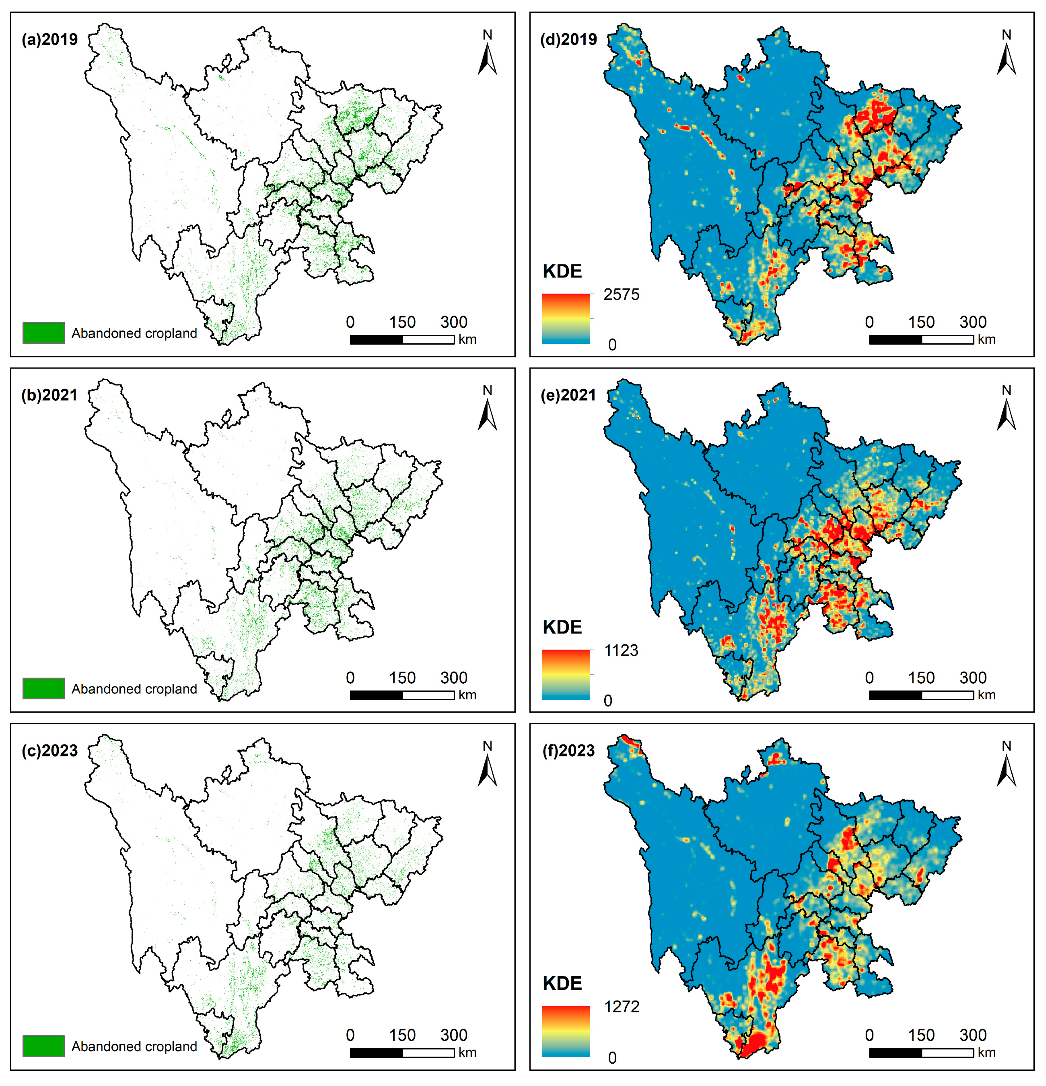
2.3.2. Kernel Density Estimation

We employed the kernel density estimation (KDE) method to analyze the spatial patterns of abandoned cropland and identify hotspots of CA distribution. KDE is a non-parametric surface density calculation method that computes the unit density of point or line feature measurements within a specified neighborhood range. It can identify various location-based characteristics and intuitively reflect the distribution of discrete measurements within a region. Compared to traditional point density estimation methods, KDE results exhibit higher continuity. The calculation formula is as follows:
f x = 1 n h i = 1 n k x x i h
where f(x) represents the kernel density estimate at point x; n represents the number of points; h represents the bandwidth; k represents the kernel function; and xxi represents the distance from the estimation point x to the sample point xi. The calculation process was implemented using the kernel density tool in the ArcGIS 10.7 platform.

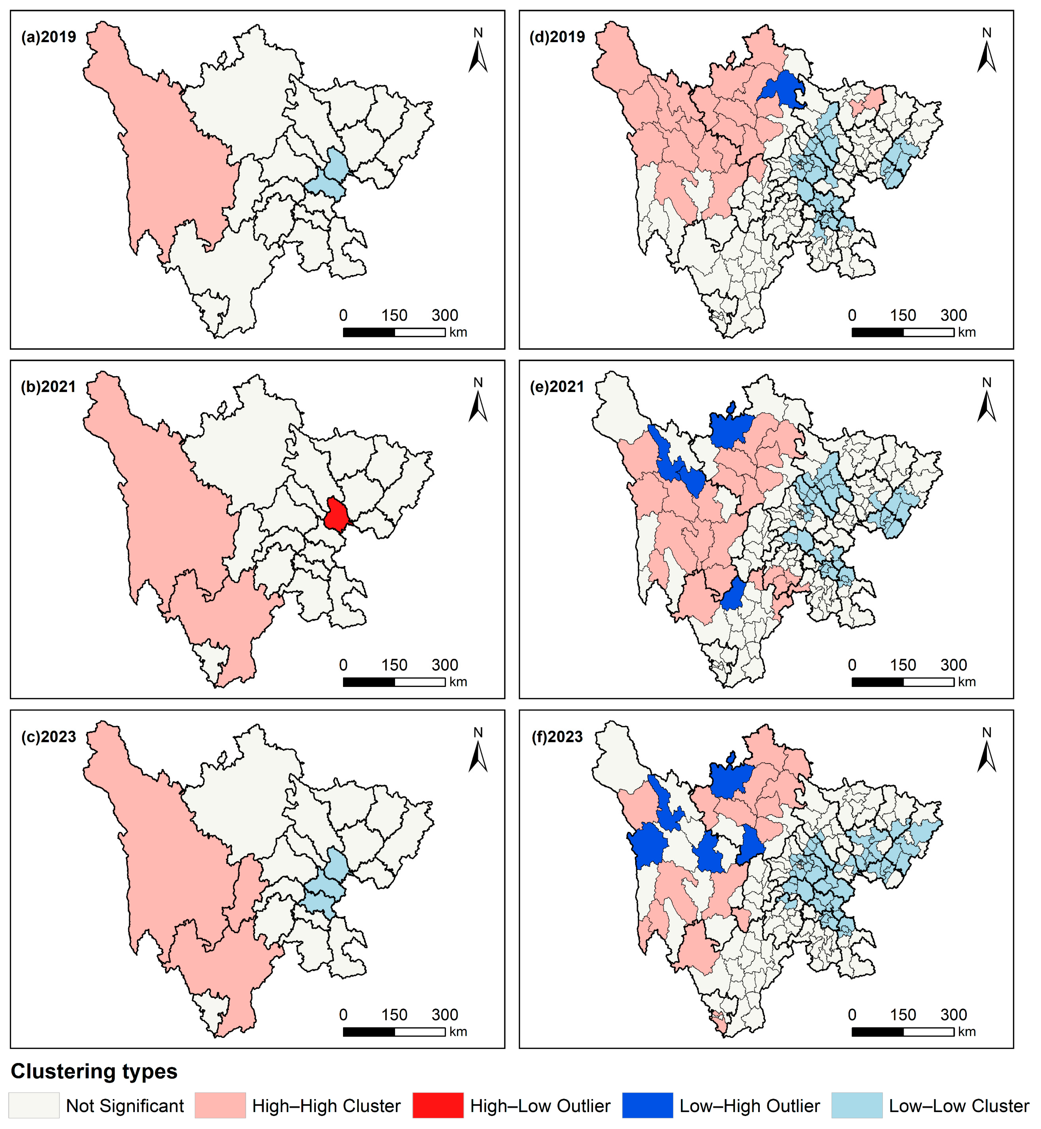
2.3.3. Global and Local Spatial Autocorrelation

Exploratory spatial data analysis (ESDA) methods were employed to reveal the spatial patterns of CA. We calculated both global and local spatial autocorrelation of CA, measured by the Moran’s I index [65,66]. Global spatial autocorrelation describes the spatial distribution characteristics of CA across the entire study area, determining whether CA exhibits clustering patterns spatially, while local spatial autocorrelation decomposes global spatial autocorrelation, revealing the similarity or dissimilarity between a spatial unit and its neighboring units in terms of feature values. The calculation formulas are as follows:
I = n i = 1 n j = 1 n w i j x i x ¯ x j x ¯ i = 1 n j = 1 n w i j i = 1 n x i x ¯ 2 , i j
I i = n x i x ¯ i = 1 n x i x ¯ 2 j = 1 n w i j x j x ¯ , i j
where I represents the global Moran’s I; n represents the number of spatial units under different administrative divisions; xi and xj represent the abandonment rates of spatial units i and j, respectively; x ¯ represents the mean abandonment rate; wij represents the spatial weight matrix; and Ii represents the local Moran’s I for spatial unit i. The value of I ranges from [−1, 1]. At a given significance level, if I is significantly greater than 0, it indicates positive spatial autocorrelation; if I is significantly less than 0, it indicates negative spatial autocorrelation; and if I is close to or equal to 0, it indicates no spatial autocorrelation. For Ii, if Ii is significantly greater than 0, it indicates that the abandonment rates of neighboring spatial units are similar (high–high or low–low); if Ii is significantly less than 0, it indicates significant differences in abandonment rates between neighboring spatial units (high–low or low–high). The spatial autocorrelation analysis was conducted using the GeoDa 1.22 software platform.

2.3.4. Hierarchical Linear Model

In social science research, the relationship between research subjects and their external environments is often characterized by mutual influence. On the one hand, external environments are shaped by individual behaviors; on the other hand, individual characteristics are influenced by external conditions. As a result, many research questions exhibit a multi-level nested data structure. When data have a hierarchical structure, traditional regression models, which analyze all data at the same level, inevitably lead to interpretative and statistical errors. To address variance decomposition issues, the hierarchical linear model (HLM) decomposes the variance in the dependent variable into two components: within-group differences (variation among individuals within the same group) and between-group differences (variation among individuals across different groups). By treating the intercepts and slopes from lower-level models as dependent variables in higher-level models, HLM can model these differences and reveal how explanatory variables at different levels influence the dependent variable in terms of their mechanisms and magnitudes of impact.
The abandonment rate (AR), which is the focus of this study, is calculated at the county level, with counties nested within municipal-level cities, forming a multi-level data structure. Therefore, this study uses HLM to measure the effects of explanatory variables at both the county level (level-1) and municipal-level city (level-2) on the AR (dependent variable). The explanatory variables, as detailed in Section 2.4, are used to assess these effects at different spatial scales. Given the availability of data, we modeled the AR for 2021 to reveal the contributions of these determinants. The calculations were carried out using HLM 7.0 software. To simplify the explanation, we illustrate the construction of the HLM with a scenario featuring one level-1 and one level-2 explanatory variable.
  • Null model
The null model is the first step in constructing an HLM. It refers to a model that does not include any explanatory variables in either the level-1 or level-2 equations. Its purpose is to decompose the total variance of the AR across the two levels and determine whether there are municipal-level city differences in county-level AR by calculating the intra-class correlation coefficient (ICC). This helps decide whether multi-level linear regression analysis is necessary. The calculation formulas are as follows:
  • Level-1
Y i j = β 0 j + r i j
  • Level-2
β 0 j = γ 00 + μ 0 j
I C C = τ 00 τ 00 + σ 2
where Yij represents the AR of county i in municipal-level city j; β0j represents the level-1 intercept associated with municipal-level city j; rij represents the level-1 residual; γ00 is the overall intercept; μ0j represents the level-2 residual; ICC is the intra-class correlation coefficient; σ2 is the variance of rij, or the within-group variance; and τ00 is the variance of μ0j, or the between-group variance. According to previous studies [59,67], an ICC < 0.059 indicates low within-group correlation, 0.059 ≤ ICC < 0.138 indicates moderate within-group correlation, and ICC ≥ 0.138 indicates high within-group correlation. When the ICC is greater than 0.059, it is necessary to construct an HLM.
2.
Random effect regression model
The random effect regression model refers to a model that includes all level-1 (county-level) explanatory variables but excludes any level-2 (municipal-level city) explanatory variables. This model aims to estimate the impact of county-level explanatory variables on the AR without the influence of municipal-level city variables, identify significant county-level influencing factors, and explore variations in the level-1 intercepts and slopes across level-2 units. The calculation formulas are as follows:
  • Level-1
Y i j = β 0 j + β 1 j X 1 i j + r i j
  • Level-2
β 0 j = γ 00 + μ 0 j
β 1 j = γ 10 + μ 1 j
where β1j represents the slope of the level-1 explanatory variable X1ij associated with municipal-level city j; X1ij represents the first explanatory variable for county i in municipal-level city j. γ10 and μ1j represent the intercept and residual of β1j, respectively. If there are additional explanatory variables at the county level, the second and third variables are denoted as X2ij and X3ij, with corresponding slopes β2j and β3j; the intercepts and residuals for β2j are γ20 and μ2j, and for β3j, they are γ30 and μ3j, and so on. The meanings of other parameters in the formula remain the same as described above.
3.
Full model
The full model includes both level-1 (county-level) and level-2 (municipal-level city) explanatory variables. This model not only explains how the overall variation in the AR is influenced by county-level and municipal-level city explanatory variables but also reveals the moderating effects of municipal-level city variables on county-level variables. The calculation formulas are as follows:
  • Level-1
Y i j = β 0 j + β 1 j X 1 i j + r i j
  • Level-2
β 0 j = γ 00 + γ 01 W 1 j + μ 0 j
β 1 j = γ 10 + γ 11 W 1 j + μ 1 j
where γ01 and γ11 represent the regression coefficients associated with W1j for β0j and β1j, respectively; and W1j represents the first explanatory variable at the municipal-level city. If there are additional explanatory variables at the municipal-level city, the second and third variables are denoted as W2j and W3j, with corresponding regression coefficients γ02 and γ03 for β0j, and γ12 and γ13 for β1j, and so on. The meanings of the other parameters in the formula are the same as those explained earlier.
To illustrate the extent to which municipal-level city explanatory variables influence the variation in county-level explanatory variables, it is necessary to calculate the proportion of the conditional variance relative to the original variance, known as the variance reduction ratio (explained variance). The calculation formula is as follows:
d = μ ^ μ ^ μ ^
where d represents the variance reduction ratio (explained variance); μ ^ represents the original variance, which is the variance component in the random results without level-2 variables; and μ ^ represents the conditional variance, which is the remaining variance component in the random results after including level-2 variables.

2.4. Explanatory Variables

Numerous studies have extensively discussed the influencing factors of CA, and although these factors vary across regions, there is a consensus that CA is the result of multi-scale and multi-factor interactions [20,52,68]. Based on a careful review of previous studies and considering the actual conditions of the study area as well as data availability, we selected 14 potential explanatory variables at both the county- and municipal-level city scales to explore the determinants of CA in the study area.
Natural factors are represented by elevation and slope, which form the fundamental background of cropland use, shape the spatial distribution of cropland resources, and influence crop types and potential yields by affecting access to sunlight and precipitation [69,70]. Flat croplands are more suitable for large-scale and mechanized farming and are less likely to be abandoned, while sloping croplands face challenges such as soil erosion, increasing the risk of abandonment [71]. We hypothesize that higher elevations and steeper slopes will increase the likelihood of CA due to harsher environmental conditions and limited agricultural accessibility. Additionally, landscape pattern characteristics, such as agglomeration and fragmentation, significantly influence cropland use practices, reflecting whether cropland distribution is conducive to cultivation, management, and cost reduction [14]. Specifically, we expect that a higher agglomeration index (AI) will decrease the probability of abandonment by facilitating agricultural operations, while a higher fragmentation index (FRA) may increase the risk of abandonment due to the difficulty in management.
While natural factors primarily influence cropland use by shaping its utilization conditions, socio-economic factors affect cropland use by influencing the income structure and migration patterns of agricultural stakeholders, thereby impacting their decision-making regarding cropland use, and these effects manifest at different spatial scales. Here, we selected relevant variables primarily from the perspectives of development level, population structure, and agricultural technology. Among these, GDP and the proportion of the secondary and tertiary industries (PSTI) reflect the overall level of economic development and the economic structure of a region. We hypothesize that higher GDP and PSTI will be associated with a greater likelihood of CA, as stronger economic development and more non-agricultural employment opportunities tend to attract labor away from agriculture, increasing the opportunity cost of farming. Areas with stronger economic strength and a higher PSTI typically offer better industrial benefits and more non-agricultural employment opportunities. Given the relatively low returns from agricultural production and the high opportunity costs, farmers may prefer to enter non-agricultural sectors, reducing their investment in agricultural production and ultimately leading to abandonment. Urbanization, a long-term national strategy in China, has brought profound changes to the country’s socio-economic structure, resulting in large-scale rural-to-urban migration. One of the most evident outcomes is the separation of people from land, exacerbating CA [72,73]. Thus, we expect that a higher urbanization rate (UR) will be positively correlated with CA, as more urbanized areas tend to experience greater labor outmigration from rural regions.
Population structure is also a critical factor influencing CA, as agricultural production in China still relies heavily on labor. The availability of agricultural labor directly determines whether cropland can be effectively utilized, and mismatches between agricultural labor and cropland increase the risk of abandonment [42,74]. We hypothesize that a larger rural population (RP) will reduce the likelihood of CA by ensuring a sufficient labor force for agricultural activities. The proportion of non-agricultural employment (PNAE) is another key indicator reflecting labor shifts from agriculture to other industries. We hypothesize that a higher PNAE will be positively associated with CA, as an increasing share of the workforce engaged in non-agricultural sectors reduces the availability of labor for farming activities, thereby increasing the risk of cropland abandonment. Total agricultural machinery power (TAMP), a proxy for agricultural technology, reflects the level of agricultural mechanization and production efficiency. Regions with higher TAMP typically indicate more advanced agriculture, where stakeholders are willing to invest more resources in cropland, resulting in a lower likelihood of abandonment. Accordingly, we expect that higher TAMP will be negatively associated with CA, as increased mechanization can compensate for labor shortages and improve land-use efficiency.
Finally, the influence of cropland location factors cannot be overlooked [31]. Here, we primarily considered the market accessibility of agricultural products and the convenience of farming, selecting variables such as the distance of cropland to townships, county administrative centers, major roads, and water sources. We hypothesize that greater distances to townships (DisT), county administrative centers (DisC), and major roads (DisR) will increase the risk of CA due to higher transportation costs and reduced market accessibility. On the other hand, cropland located closer to water sources (DisW) may be more suitable for irrigation, thereby decreasing the likelihood of abandonment.
Table 2 lists all potential explanatory variables and their descriptive statistics.

3. Results

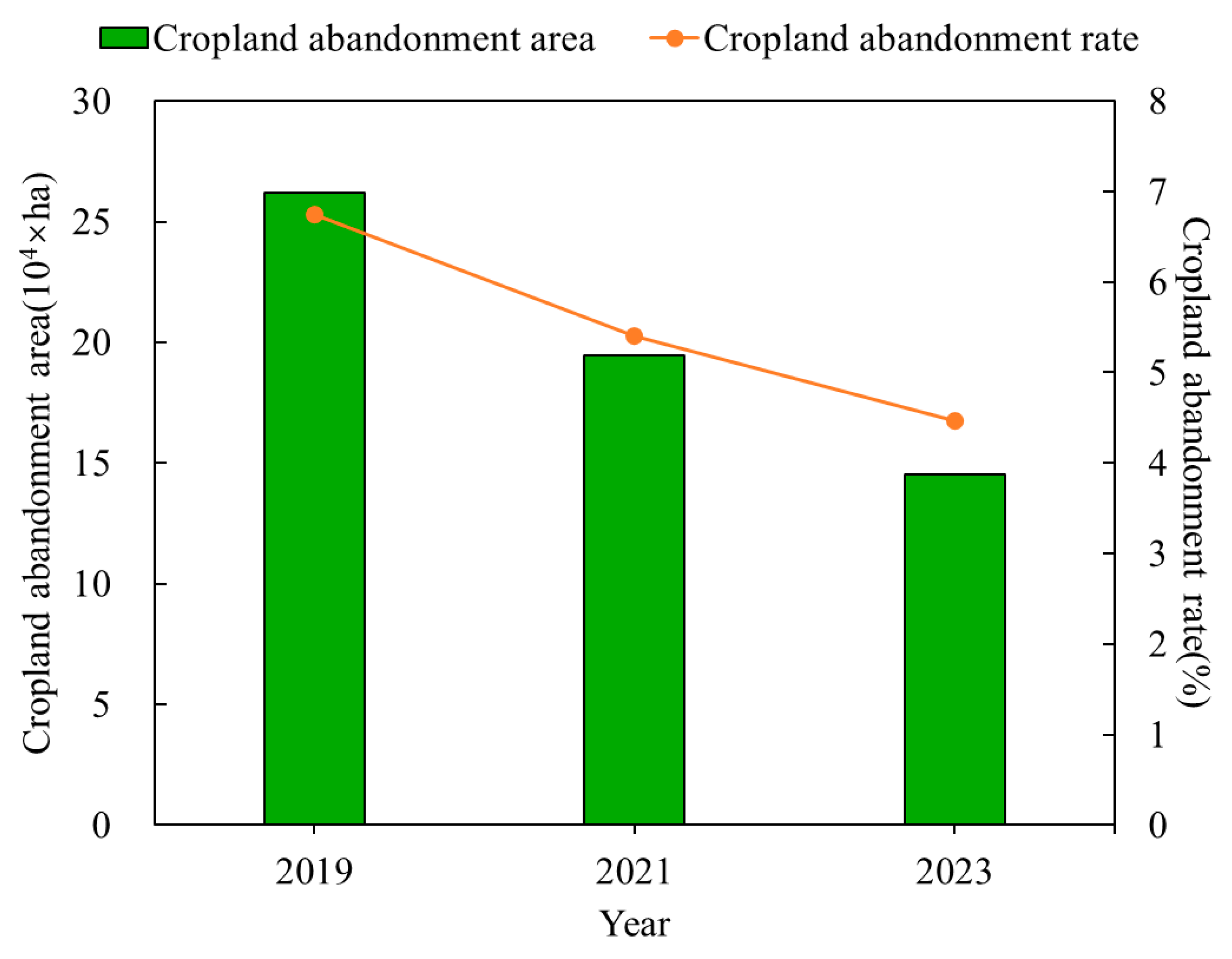
3.1. Spatiotemporal Patterns of Cropland Abandonment in Sichuan Province

In terms of the scale of CA (Figure 3), the abandoned cropland area in Sichuan Province in 2019, 2021, and 2023 was 26.21 × 10⁴ ha, 19.46 × 10⁴ ha, and 14.54 × 10⁴ ha, respectively. The corresponding abandonment rates were 6.75%, 5.40%, and 4.47%, showing a continuous downward trend overall.
From the perspective of the spatiotemporal patterns of CA, abandoned cropland in Sichuan exhibits significant clustering characteristics. The spatial autocorrelation analysis results show that the global Moran’s I for all three years is greater than 0 at both the municipal-level city and county scales, with the clustering degree at the county scale being significantly higher than that at the municipal-level city scale. However, over time, the clustering degree at the municipal-level city scale has increased, while it has decreased at the county scale (Table 3). High-value clusters of abandonment rates are primarily distributed in the western mountainous regions of Sichuan, while low-value clusters are mainly concentrated in the eastern plains and peripheral hilly areas of the basin (Figure 4).
Overall, the spatial distribution of CA in Sichuan exhibits a clear gradient differentiation pattern, where the AR gradually increases as the terrain rises from the southeast to the northwest (Figure 1). However, over time, although the AR in the western regions generally remains above 15%, it has shown a slowdown, while the AR in the eastern regions has largely stayed below 5% (Figure 5). Additionally, there are significant differences in abandonment rates among cities and counties within Sichuan, but these disparities are gradually narrowing. At the municipal-level city scale, in 2019, the abandonment rates across cities ranged from 1.32% to 38.77%, with an average of 10.49% and a standard deviation of 10.10%; the minimum and maximum values occurred in Deyang City and Ganzi Prefecture, respectively. In 2021, the abandonment rates ranged from 1.76% to 15.45%, with the average significantly decreasing to 6.92% and a standard deviation of 3.87%; the minimum and maximum values were observed in Deyang City and Ya’an City, respectively. In 2023, the abandonment rates ranged from 1.01% to 27.57%, with the average slightly decreasing to 6.79% and a standard deviation of 7.17%; the minimum and maximum values occurred in Guang’an City and Aba Prefecture, respectively. At the county scale, the average abandonment rates in 2019, 2021, and 2023 were 14.37%, 9.95%, and 9.79%, respectively, with standard deviations of 16.71%, 8.71%, and 11.37%.
The calculation method for the AR eliminates the influence of differences in baseline cropland area, facilitating both vertical and horizontal comparisons across spatial units at different administrative levels. However, it provides limited information, whereas grid-scale analysis can capture more details about CA. Although we generated a 10 m resolution CA map, overall observation remains challenging. The KDE method effectively addresses this issue. As expected, Figure 6 reveals an interesting phenomenon. Combining this with previous analyses, we find that the severe CA situation in the western mountainous regions of Sichuan is closely related to their baseline cropland area. Represented by Aba Prefecture, Ganzi Prefecture, Liangshan Prefecture, and Panzhihua City in the western region, these areas collectively account for only about 15% of the province’s total cropland (14.64% in 2017, 15.41% in 2019, and 14.66% in 2021). This means that, compared to other regions, fluctuations in CA within this region have a more sensitive impact on the AR. Moreover, abandoned cropland tends to be spatially dispersed, with hotspots appearing mainly in localized zones, such as the eastern and southern parts of Liangshan Prefecture and the northern parts of Ganzi and Aba Prefectures. In contrast, in the eastern part of the study area, although abandoned cropland is widespread, its share relative to the baseline cropland area is smaller, resulting in lower abandonment rates, but the trend of concentrated and contiguous distribution is more pronounced. Additionally, it is noteworthy that over time, the hotspots of CA in the study area generally show a trend of migration from the northeast to the southwest, while in the eastern region, the hotspots tend to become more dispersed.

3.2. Determinants of Cropland Abandonment in Sichuan Province

3.2.1. Estimated Results of Null Model

The estimation results of the null model (Table 4) show that both the fixed effect and random effect of the model passed the significance test (p < 0.01). The within-group variance and between-group variance are 44.4254 and 28.1214, respectively. This indicates that 38.76% of the variation in county-level abandonment rates in 2021 is attributed to differences among municipal-level cities, while the remaining 61.24% stems from heterogeneity among counties. Although county-level differences dominate, the influence of municipal-level city factors on the AR cannot be overlooked. Additionally, the intra-class correlation coefficient (ICC) is 0.3876, which is greater than 0.138, indicating a high level of within-group correlation. Therefore, it is necessary to construct an HLM to comprehensively analyze the influencing factors of the AR at both the county- and municipal-level city scales.

3.2.2. Estimated Results of Random Effect Regression Model

Before constructing the random effect regression model, this study first conducted a multicollinearity test for county-level variables. Based on the variance inflation factor (VIF), indicators with strong collinearity (e.g., GDP) were removed. The estimation results of the random effect regression model (Table 5) show that, in terms of the model’s fixed effect, the agglomeration index (AI) is a key determinant of CA and has a highly significant negative impact on CA (regression coefficient = −0.3681, p < 0.01). This indicates that the higher the degree of cropland aggregation, the lower the AR. Concentrated and contiguous cropland is more suitable for mechanization and can reduce production costs and increase profits through large-scale cultivation, thereby lowering the likelihood of abandonment. DEM (regression coefficient = 0.0023, p < 0.1) and distance to roads (DisR, regression coefficient = 0.0028, p < 0.05) have relatively significant positive effects on CA, meaning that the higher the elevation of the cropland and the farther it is from roads, the higher the AR. Other factors did not pass the significance test and were therefore not included in subsequent models.
The random effect regression model serves two purposes: first, to determine whether level-1 variables have a significant impact on the AR, and second, and more importantly, to assess whether the regression coefficients of first-level variables exhibit significant differences at the level-2, specifically in terms of variance. The significance of the regression coefficients in the fixed effects part of the model is unrelated to the construction of the level-2 model; rather, the decision to build the level-2 model is primarily based on the significance of the variance components. From the random effect results of the model, the chi-square test for the intercept term is significant (variance component = 30.5020, p < 0.01), indicating that the average AR varies significantly among municipal-level cities. Therefore, it is necessary to include municipal-level city variables in the full model to analyze contextual effects. Additionally, the chi-square test for the variance component of AI is significant (variance component = 0.0846, p < 0.01), indicating that the negative impact of AI on the AR also varies significantly among municipal-level cities. Thus, it is necessary to construct a corresponding level-2 model using this regression coefficient as the dependent variable. Furthermore, it should be noted that when we attempted to include the random slopes of the four location-related explanatory variables (DisT, DisC, DisR, and DisW) in the model, the estimates did not converge at all. This aligns with previous research experiences [48,75]. Since there is no argument suggesting that the relationship between explanatory variables and the dependent variable would differ when random slopes are included, these four explanatory variables only have fixed effect estimates and no random effect estimates.

3.2.3. Estimated Results of Full Model

Based on the analysis results of the random effect regression model, we constructed the full model (Formulas (15)–(19)). Among them, GDP was excluded due to the issue of multicollinearity.
  • Level-1
Y = β 0 + β 1 D E M + β 2 A I + β 3 D i s R + r
  • Level-2
β 0 = γ 00 + γ 01 P S T I + γ 02 U R + γ 03 P N A E + μ 0
β 1 = γ 10
β 2 = γ 20 + γ 21 P S T I + γ 22 U R + γ 23 P N A E + μ 2
β 3 = γ 30
The estimation results of the full model (Table 6) show that the influence of county-level explanatory variables on the AR in the full model is similar to the results of the random effect regression model, with consistent trends. Among them, DEM and DisR have highly significant positive effects on the AR (p < 0.01), with only minor changes in the regression coefficients. AI has a relatively significant negative effect on the AR, and its impact has noticeably increased (the absolute value of the regression coefficient rose from 0.3681 to 1.5669), although the significance level has decreased. Meanwhile, the variables UR (urbanization rate) and PNAE (proportion of non-agricultural employment), which were not significant in the random effect regression model, have highly significant positive effects on the AR in the full model (p < 0.01), with regression coefficients of 0.4501 and 0.6441, respectively. This indicates that an increase in the UR and the PNAE at the municipal level leads to an increase in the AR at the county level. The above results suggest that the inclusion of municipal-level explanatory variables not only has a direct impact on the AR but also plays a moderating role. Further examination of this moderating effect reveals that the regression coefficients of the municipal-level variables PSTI (proportion of secondary and tertiary industries), UR, and PNAE have opposite signs to the regression coefficient of AI at the county level, indicating that these three municipal-level variables weaken the effect of AI on the AR. Among these, only the regression coefficient of PNAE passed the significance test (p < 0.05), meaning that an increase in the proportion of non-agricultural employment reduces the negative impact of AI on the AR. Furthermore, comparing the variance components of the random effect model and calculating the variance reduction ratio reveals that 57% of the differences in county-level AR means ((30.5020 − 13.1717)/30.5020) can be explained by municipal-level PSTI, UR, and PNAE.

4. Discussion

4.1. Comparison with Existing Studies

Understanding the distribution and spatial patterns of abandoned cropland is crucial for assessing its socio-ecological consequences and exploring its potential contributions to food production and bioenergy. Using deep learning methods, we derived land-use change information from Sentinel-2 data to map high-resolution abandoned cropland in Sichuan, China, and identified hotspots of abandonment. Compared to similar studies, our results show some differences. For instance, our findings indicate an average AR of approximately 5.54% (averaged across 2019, 2021, and 2023), with rates exceeding 15% in the western mountainous regions. In contrast, a remote sensing study in Chongqing, a neighboring region with 76% mountainous and hilly terrain, reported an AR of 6.45% from 2000 to 2020 [15]. Another case study in southern Sichuan observed an increase in abandonment rates from 2% in 2003 to 15% in 2018 [50]. These discrepancies may arise from differences in the quality of land cover datasets, definitions of abandonment, and study periods. However, our use of 10 m resolution remote sensing data likely provides a more accurate assessment.
In terms of spatial patterns, our maps confirm the general trend that abandonment rates are significantly higher in mountainous areas compared to other terrains [14,26,29]. We also highlight a less-discussed detail: the severe abandonment in mountainous regions may be linked to their relatively small baseline cropland area, as almost all remote sensing studies use the ratio of abandoned cropland to baseline cropland as a key indicator of abandonment intensity.
Additionally, our study emphasizes the slowing trend of abandonment in mountainous areas, which contrasts with some existing studies [27,35,50]. However, this finding is reasonable and well supported. Mountainous agricultural systems, with limited resilience and adaptability, are considered highly vulnerable to abandonment [8]. This also means that abandonment in these areas receives significant attention, leading to targeted governance measures. In China, food security is a critical component of national security, and the retention of cropland area is tied to the performance evaluations of provincial leaders, making any unexpected reduction in cropland unacceptable. To address widespread abandonment, the Chinese government introduced specific policies in 2021, particularly targeting hilly and mountainous regions, resulting in a recent trend of re-cultivating abandoned cropland, which aligns with our study period. Thus, the decline in abandonment rates in mountainous areas is foreseeable.
Overall, while direct quantitative comparisons with other studies are challenging, our results underscore the difficulty in mapping abandoned cropland at large scales, especially in mountainous regions with mixed pixels and highly heterogeneous land-use patterns. The use of long-term, high-resolution remote sensing data is essential for improving the accuracy of abandonment detection in these areas.

4.2. Determinants of Cropland Abandonment

Understanding the determinants of CA provides valuable guidance for identifying effective land restoration pathways. Most studies focus on influencing factors at a single level [28,30,31] or separately estimate factors at different levels [50,76,77]. However, since abandonment results from multi-level factors, these studies often lack a comprehensive understanding of the underlying mechanisms.
By introducing HLM to abandonment research, our study not only identifies determinants at both county and municipal scales but also reveals their interactions. Our results show that at the county level, a higher AI corresponds to lower abandonment rates, while DEM and distance to roads have significant positive effects. At the municipal scale, UR and PNAE are statistically significant factors, which is consistent with previous studies [14,37,43], indicating that natural, socio-economic, and locational factors play crucial roles in the spatial heterogeneity of abandonment.
Additionally, leveraging the advantages of HLM, we found that an increase in PNAE weakens the negative impact of AI on abandonment rates. This can be explained by the fragmentation of cropland property rights in China. To ensure fairness, cropland allocation follows a principle of “mixing fertile and less fertile plots”, meaning that households often own scattered plots of varying quality. As more households shift to non-farm employment, their desire to increase household income not only directly leads to abandonment but also indirectly reduces the mitigating effect of AI on abandonment. This is because any attempt to utilize contiguous cropland at scale—whether by economically capable households or specialized organizations—requires negotiating with multiple property owners, increasing transaction costs and diminishing the negative impact of AI on abandonment rates.
While our study effectively captures the determinants of CA at the county and municipal levels, it is important to acknowledge that micro-level factors, such as population aging, land transfer mechanisms, and social services, also play a crucial role in shaping abandonment patterns. Existing research suggests that aging rural populations often exhibit a lower willingness to cultivate land, and in some cases, prefer abandonment over transferring land-use rights, particularly in hilly and mountainous areas where farming is labor-intensive [78]. Our study does not directly incorporate aging as a variable, but our findings on urbanization and non-agricultural employment indirectly reflect its impact, as younger generations tend to migrate to urban areas, leaving behind an aging agricultural workforce. Future research could further integrate aging-specific metrics to refine the analysis.
Similarly, land transfer has been widely recognized as a potential mechanism for mitigating cropland abandonment [79]. However, its effects are highly context-dependent. For instance, in peri-urban areas, proximity to cities often facilitates land acquisition for non-agricultural purposes, which may accelerate abandonment rather than reduce it [80]. Moreover, the role of new agricultural operating entities, such as cooperatives and agribusinesses, was highlighted as a crucial factor in farmland utilization [81]. These entities can reduce abandonment by consolidating small plots into larger, more manageable units. However, their effectiveness is constrained by land tenure security, transaction costs, and the willingness of smallholders to participate in collective farming.
Additionally, social services and rural infrastructure significantly influence CA but were not explicitly examined in our study. Prior research indicates that access to agricultural extension services, rural credit programs, and irrigation facilities can substantially impact farmers’ decisions to maintain or abandon cropland [50,82,83]. Regions with better-developed rural services may exhibit lower abandonment rates, as farmers receive greater institutional support to sustain agricultural activities. This aspect could be further explored in future studies by incorporating detailed spatial data on rural service provision.
Overall, our study provides new insights into the multi-scale determinants of abandonment, which may help better curb abandonment, a challenge faced by many regions worldwide. At the same time, acknowledging the role of micro-level factors—such as aging, land transfer, and rural social services—can further enhance our understanding of CA dynamics. Future studies could benefit from integrating these aspects through household surveys or fine-scale socio-economic data, complementing the macro- and meso-level analyses presented here.

4.3. Policy Implications

Appropriate farming conditions are essential for ensuring the long-term sustainable use of cropland. Our results highlight AI as a key determinant. Therefore, effective measures include consolidating fragmented cropland plots, improving soil quality and fertility, and investing in irrigation and field road infrastructure to enhance agricultural conditions and support large-scale, mechanized farming.
Given the ongoing urbanization in China, particularly in remote mountainous areas, agricultural labor will continue to decline, and the proportion of households engaged in non-farm employment will increase, leading to persistent abandonment. A promising approach is to facilitate the transfer of abandoned cropland to active users through leasing or exchange, enabling efficient and profitable utilization. This requires introducing or cultivating large-scale agricultural entities, such as renowned agricultural enterprises and cooperatives, while improving rural land transfer services and markets to reduce transaction costs and promote concentrated development. Additionally, high-value crops such as fruits, medicinal herbs, and tea should be promoted in mountainous areas to diversify and enhance product offerings. Further research is needed to clarify reutilization plans for abandoned cropland, addressing trade-offs among food security, household livelihoods, and ecosystem services such as biodiversity and carbon storage.
Finally, we recommend strengthening legal mechanisms to combat abandonment, including reclaiming abandoned cropland and suspending agricultural subsidies for abandoned land, while enhancing monitoring through remote sensing, drones, and ground inspections to promptly detect and respond to abandonment.

4.4. Limitations

While deep learning methods have significantly advanced land cover classification compared to traditional remote sensing approaches, challenges remain in abandonment detection.
Firstly, defining abandonment solely based on land cover changes may not fully reflect actual abandonment. For example, some cropland may be intermittently cultivated due to labor shortages or low economic returns, appearing as active cropland in land cover data but effectively “semi-abandoned”. Similarly, cropland converted to other agricultural uses (e.g., orchards) may be misclassified as abandoned.
Secondly, despite using advanced deep learning methods, classification uncertainties can affect the accuracy of abandonment detection. As shown in Table 7, while the model achieved high overall accuracy (85.3%) and a Kappa coefficient of 0.81, classification accuracy varied among land cover types. In mountainous areas, challenges such as fragmented plots, shadow interference, and mixed pixels may lead to misclassification, with errors amplified in multi-temporal analyses, affecting the reliability of abandonment detection.
Despite these limitations, remote sensing-based methods remain effective for large-scale studies of abandonment, providing cost-effective, continuous, and spatially extensive data. Future research can improve accuracy by integrating multi-source data, refining classification methods, and enhancing ground validation.

5. Conclusions

Understanding the location, scale, patterns, and determinants of CA in mountainous areas is critical, as these regions offer greater restoration potential and more diverse restoration options compared to plains, especially in a country like China with its vast population and predominantly mountainous terrain. Using remote sensing data, we mapped high-resolution abandoned cropland in Sichuan, applied KDE and spatial autocorrelation methods to reveal spatiotemporal patterns, and employed HLM to explore determinants at county- and municipal-level city scales.
Our results show that abandonment rates in Sichuan decreased from 6.75% in 2019 to 4.47% in 2023, with significant spatial clustering at both county- and municipal-level city scales. High-value clusters were concentrated in the western mountainous regions, while low-value clusters were found in the eastern plains and peripheral hilly areas. Grid-scale analysis revealed a northeast-to-southwest migration of abandonment hotspots.
At the county level, AI was a key determinant, with DEM and distance to roads also showing significant positive effects. At the municipal city level, UR and PNAE increased abandonment rates, while PNAE weakened the negative impact of AI due to fragmented property rights.
Our study provides high-resolution insights into abandonment in mountainous regions, offering valuable information for policymakers to design effective reutilization strategies for abandoned cropland.

Author Contributions

Conceptualization, B.H., J.W. and P.R.; methodology, B.H., J.W. and J.X.; formal analysis, B.H.; data curation, B.H. and J.W.; writing—original draft preparation, B.H.; writing—review and editing, B.H., J.W., J.X., Q.Y. and P.R.; visualization, B.H. and J.W.; supervision, P.R.; project administration, P.R.; funding acquisition, P.R. All authors have read and agreed to the published version of the manuscript.

Funding

This research was funded by the Sichuan Science and Technology Program (grant No. 2023NSFSC1979) and the National Social Science Foundation of China (grant No. 18XJY010).

Data Availability Statement

Data are available from the authors upon reasonable request.

Conflicts of Interest

The authors declare no conflicts of interest.

References

  1. UN. Transforming our World: The 2030 Agenda for Sustainable Development. 2015. Available online: https://sdgs.un.org/sites/default/files/publications/21252030%20Agenda%20for%20Sustainable%20Development%20web.pdf (accessed on 2 December 2024).
  2. UN. The Sustainable Development Goals Report 2024. 2024. Available online: https://unstats.un.org/sdgs/report/2024/The-Sustainable-Development-Goals-Report-2024.pdf (accessed on 2 December 2024).
  3. Estel, S.; Kuemmerle, T.; Alcántara, C.; Levers, C.; Prishchepov, A.; Hostert, P. Mapping Farmland Abandonment and Recultivation across Europe Using MODIS NDVI Time Series. Remote Sens. Environ. 2015, 163, 312–325. [Google Scholar] [CrossRef]
  4. Næss, J.S.; Cavalett, O.; Cherubini, F. The Land–Energy–Water Nexus of Global Bioenergy Potentials from Abandoned Cropland. Nat. Sustain. 2021, 4, 525–536. [Google Scholar] [CrossRef]
  5. Huang, W.; Hashimoto, S.; Yoshida, T.; Saito, O.; Meraj, G. Understanding Japan’s Land-Use Dynamics between 1987 and 2050 Using Land Accounting and Scenario Analysis. Sustain. Sci. 2024, 19, 1561–1577. [Google Scholar] [CrossRef]
  6. Xie, Y.; Spawn-Lee, S.A.; Radeloff, V.C.; Yin, H.; Robertson, G.P.; Lark, T.J. Cropland Abandonment between 1986 and 2018 across the United States: Spatiotemporal Patterns and Current Land Uses. Environ. Res. Lett. 2024, 19, 044009. [Google Scholar] [CrossRef]
  7. Zheng, Q.; Ha, T.; Prishchepov, A.V.; Zeng, Y.; Yin, H.; Koh, L.P. The Neglected Role of Abandoned Cropland in Supporting Both Food Security and Climate Change Mitigation. Nat. Commun. 2023, 14, 6083. [Google Scholar] [CrossRef]
  8. Haddaway, N.R.; Styles, D.; Pullin, A.S. Evidence on the Environmental Impacts of Farm Land Abandonment in High Altitude/Mountain Regions: A Systematic Map. Environ. Evid. 2014, 3, 17. [Google Scholar] [CrossRef]
  9. Ojha, R.B.; Atreya, K.; Kristiansen, P.; Devkota, D.; Wilson, B. A Systematic Review and Gap Analysis of Drivers, Impacts, and Restoration Options for Abandoned Croplands in Nepal. Land Use Policy 2022, 120, 106237. [Google Scholar] [CrossRef]
  10. Queiroz, C.; Beilin, R.; Folke, C.; Lindborg, R. Farmland Abandonment: Threat or Opportunity for Biodiversity Conservation? A Global Review. Front. Ecol. Environ. 2014, 12, 288–296. [Google Scholar] [CrossRef]
  11. Novara, A.; Gristina, L.; Sala, G.; Galati, A.; Crescimanno, M.; Cerda, A.; Badalamenti, E.; La Mantia, T. Agricultural Land Abandonment in Mediterranean Environment Provides Ecosystem Services via Soil Carbon Sequestration. Sci. Total Environ. 2017, 576, 420–429. [Google Scholar] [CrossRef]
  12. Crawford, C.L.; Yin, H.; Radeloff, V.C.; Wilcove, D.S. Rural Land Abandonment Is Too Ephemeral to Provide Major Benefits for Biodiversity and Climate. Sci. Adv. 2022, 8, eabm8999. [Google Scholar] [CrossRef]
  13. Chen, H.; Tan, Y.; Xiao, W.; He, T.; Xu, S.; Meng, F.; Li, X.; Xiong, W. Assessment of Continuity and Efficiency of Complemented Cropland Use in China for the Past 20 Years: A Perspective of Cropland Abandonment. J. Clean. Prod. 2023, 388, 135987. [Google Scholar] [CrossRef]
  14. Guo, A.; Yue, W.; Yang, J.; Xue, B.; Xiao, W.; Li, M.; He, T.; Zhang, M.; Jin, X.; Zhou, Q. Cropland Abandonment in China: Patterns, Drivers, and Implications for Food Security. J. Clean. Prod. 2023, 418, 138154. [Google Scholar] [CrossRef]
  15. Li, S.; Xiao, J.; Lei, X.; Wang, Y. Farmland Abandonment in the Mountainous Areas from an Ecological Restoration Perspective: A Case Study of Chongqing, China. Ecol. Indic. 2023, 153, 110412. [Google Scholar] [CrossRef]
  16. Zabel, F.; Delzeit, R.; Schneider, J.M.; Seppelt, R.; Mauser, W.; Vaclavik, T. Global Impacts of Future Cropland Expansion and Intensification on Agricultural Markets and Biodiversity. Nat. Commun. 2019, 10, 2844. [Google Scholar] [CrossRef] [PubMed]
  17. Lark, T.J.; Spawn, S.A.; Bougie, M.; Gibbs, H.K. Cropland Expansion in the United States Produces Marginal Yields at High Costs to Wildlife. Nat. Commun. 2020, 11, 4295. [Google Scholar] [CrossRef]
  18. Foucher, A.; Tassano, M.; Chaboche, P.-A.; Chalar, G.; Cabrera, M.; Gonzalez, J.; Cabral, P.; Simon, A.-C.; Agelou, M.; Ramon, R.; et al. Inexorable Land Degradation Due to Agriculture Expansion in South American Pampa. Nat. Sustain. 2023, 6, 662–670. [Google Scholar] [CrossRef]
  19. Jayne, T.S.; Sanchez, P.A. Agricultural Productivity Must Improve in Sub-Saharan Africa. Science 2021, 372, 1045–1047. [Google Scholar] [CrossRef]
  20. Subedi, Y.R.; Kristiansen, P.; Cacho, O. Drivers and Consequences of Agricultural Land Abandonment and Its Reutilisation Pathways: A Systematic Review. Environ. Dev. 2022, 42, 100681. [Google Scholar] [CrossRef]
  21. Gvein, M.H.; Hu, X.; Næss, J.S.; Watanabe, M.D.B.; Cavalett, O.; Malbranque, M.; Kindermann, G.; Cherubini, F. Potential of Land-Based Climate Change Mitigation Strategies on Abandoned Cropland. Commun Earth Environ. 2023, 4, 39. [Google Scholar] [CrossRef]
  22. Deininger, K.; Savastano, S.; Carletto, C. Land Fragmentation, Cropland Abandonment, and Land Market Operation in Albania. World Dev. 2012, 40, 2108–2122. [Google Scholar] [CrossRef]
  23. Wang, J.; Cao, Y.; Fang, X.; Li, G.; Cao, Y. Does Land Tenure Fragmentation Aggravate Farmland Abandonment? Evidence from Big Survey Data in Rural China. J. Rural Stud. 2022, 91, 126–135. [Google Scholar] [CrossRef]
  24. Zheng, L.; Su, L.; Jin, S. Reducing Land Fragmentation to Curb Cropland Abandonment: Evidence from Rural China. Can. J. Agric. Econ./Rev. Can. D’Agroecon. 2023, 71, 355–373. [Google Scholar] [CrossRef]
  25. Löw, F.; Prishchepov, A.V.; Waldner, F.; Dubovyk, O.; Akramkhanov, A.; Biradar, C.; Lamers, J.P.A. Mapping Cropland Abandonment in the Aral Sea Basin with MODIS Time Series. Remote Sens. 2018, 10, 159. [Google Scholar] [CrossRef]
  26. Zhu, X.; Xiao, G.; Zhang, D.; Guo, L. Mapping Abandoned Farmland in China Using Time Series MODIS NDVI. Sci. Total Environ. 2021, 755, 142651. [Google Scholar] [CrossRef]
  27. Wang, J.; Guan, Y.; Wang, H.; Zhou, W. Identifying and Monitoring of Abandoned Farmland in Key Agricultural Production Areas on the Qinghai-Tibet Plateau: A Case Study of the Huangshui Basin. J. Environ. Manag. 2024, 354, 120380. [Google Scholar] [CrossRef]
  28. Zhang, Y.; Li, X.; Song, W.; Thai, L. Land Abandonment under Rural Restructuring in China Explained from a Cost-Benefit Perspective. J. Rural Stud. 2016, 47, 524–532. [Google Scholar] [CrossRef]
  29. He, Y.; Xie, H.; Peng, C. Analyzing the Behavioural Mechanism of Farmland Abandonment in the Hilly Mountainous Areas in China from the Perspective of Farming Household Diversity. Land Use Pol. 2020, 99, 104826. [Google Scholar] [CrossRef]
  30. Gorgan, M.; Bavorova, M.; Ullah, A.; Prishchepov, A. The Role of Land Market in Shaping Farmland Abandonment in Post-Soviet Armenia. Land Use Pol. 2024, 146, 107308. [Google Scholar] [CrossRef]
  31. Chen, H.; Tan, Y.; Xiao, W.; Xu, S.; Xia, H.; Ding, G.; Xia, H.; Prishchepov, A.V. Spatiotemporal Variation in Determinants of Cropland Abandonment across Yangtze River Economic Belt, China. Catena 2024, 245, 108326. [Google Scholar] [CrossRef]
  32. Alcantara, C.; Kuemmerle, T.; Baumann, M.; Bragina, E.V.; Griffiths, P.; Hostert, P.; Knorn, J.; Mueller, D.; Prishchepov, A.V.; Schierhorn, F.; et al. Mapping the Extent of Abandoned Farmland in Central and Eastern Europe Using MODIS Time Series Satellite Data. Environ. Res. Lett. 2013, 8, 035035. [Google Scholar] [CrossRef]
  33. Dara, A.; Baumann, M.; Kuemmerle, T.; Pflugmacher, D.; Rabe, A.; Griffiths, P.; Hoelzel, N.; Kamp, J.; Freitag, M.; Hostert, P. Mapping the Timing of Cropland Abandonment and Recultivation in Northern Kazakhstan Using Annual Landsat Time Series. Remote Sens. Environ. 2018, 213, 49–60. [Google Scholar] [CrossRef]
  34. Li, L.; Pan, Y.; Zheng, R.; Liu, X. Understanding the Spatiotemporal Patterns of Seasonal, Annual, and Consecutive Farmland Abandonment in China with Time-Series MODIS Images during the Period 2005–2019. Land Degrad. Dev. 2022, 33, 1608–1625. [Google Scholar] [CrossRef]
  35. Zhang, M.; Li, G.; He, T.; Zhai, G.; Guo, A.; Chen, H.; Wu, C. Reveal the Severe Spatial and Temporal Patterns of Abandoned Cropland in China over the Past 30 Years. Sci. Total Environ. 2023, 857, 159591. [Google Scholar] [CrossRef]
  36. Zeng, J.; Luo, T.; Chen, W.; Gu, T. Assessing and Mapping Cropland Abandonment Risk in China. Land Degrad. Dev. 2024, 35, 2738–2753. [Google Scholar] [CrossRef]
  37. Li, S.; Li, X.; Sun, L.; Cao, G.; Fischer, G.; Tramberend, S. An Estimation of the Extent of Cropland Abandonment in Mountainous Regions of China. Land Degrad. Dev. 2018, 29, 1327–1342. [Google Scholar] [CrossRef]
  38. Song, W.; Yang, D.; Wang, Y. Integrating an Abandoned Farmland Simulation Model (AFSM) Using System Dynamics and CLUE-S for Sustainable Agriculture. Agric. Syst. 2024, 219, 104063. [Google Scholar] [CrossRef]
  39. Meyfroidt, P.; Schierhorn, F.; Prishchepov, A.V.; Mueller, D.; Kuemmerle, T. Drivers, Constraints and Trade-Offs Associated with Recultivating Abandoned Cropland in Russia, Ukraine and Kazakhstan. Glob. Environ. Change-Hum. Policy Dimens. 2016, 37, 1–15. [Google Scholar] [CrossRef]
  40. Movahedi, R.; Jawanmardi, S.; Azadi, H.; Goli, I.; Viira, A.-H.; Witlox, F. Why Do Farmers Abandon Agricultural Lands? The Case of Western Iran. Land Use Pol. 2021, 108, 105588. [Google Scholar] [CrossRef]
  41. Zhou, H.; Wang, J.; Sun, M.; Wang, J.; Yang, K. Evolution of Farmland Abandonment Research from 1993 to 2023 Using CiteSpace-Based Scientometric Analysis. J. Geovis. Spat. Anal. 2024, 8, 20. [Google Scholar] [CrossRef]
  42. Xu, D.; Deng, X.; Guo, S.; Liu, S. Labor Migration and Farmland Abandonment in Rural China: Empirical Results and Policy Implications. J. Environ. Manag. 2019, 232, 738–750. [Google Scholar] [CrossRef]
  43. Qiu, B.; Yang, X.; Tang, Z.; Chen, C.; Li, H.; Berry, J. Urban Expansion or Poor Productivity: Explaining Regional Differences in Cropland Abandonment in China during the Early 21st Century. Land Degrad. Dev. 2020, 31, 2540–2551. [Google Scholar] [CrossRef]
  44. Hou, D.; Meng, F.; Prishchepov, A.V. How Is Urbanization Shaping Agricultural Land-Use? Unraveling the Nexus between Farmland Abandonment and Urbanization in China. Landsc. Urban Plan. 2021, 214, 104170. [Google Scholar] [CrossRef]
  45. Ding, G.; Ding, M.; Xie, K.; Li, J. Driving Mechanisms of Cropland Abandonment from the Perspectives of Household and Topography in the Poyang Lake Region, China. Land 2022, 11, 939. [Google Scholar] [CrossRef]
  46. Wang, X.; Zhao, D. Study on the Causes of Differences in Cropland Abandonment Levels among Farming Households Based on Hierarchical Linear Model-13,120 Farming Households in 26 Provinces of China as an Example. Land 2023, 12, 1791. [Google Scholar] [CrossRef]
  47. Long, M.; Zhao, Y.; Zhou, C.; Li, X.; Su, L.; Zou, Y. Analysis of Factors Influencing Terrace Abandonment Based on Unmanned Aerial Photography and Farmer Surveys: A Case Study in Jianhe, Guizhou. Land Degrad. Dev. 2024, 35, 757–771. [Google Scholar] [CrossRef]
  48. Zhang, Y.; Li, X.; Song, W. Determinants of Cropland Abandonment at the Parcel, Household and Village Levels in Mountain Areas of China: A Multi-Level Analysis. Land Use Pol. 2014, 41, 186–192. [Google Scholar] [CrossRef]
  49. Zhou, T.; Koomen, E.; Ke, X. Determinants of Farmland Abandonment on the Urban-Rural Fringe. Environ. Manag. 2020, 65, 369–384. [Google Scholar] [CrossRef]
  50. Hong, C.; Prishchepov, A.; Bavorova, M. Cropland Abandonment in Mountainous China: Patterns and Determinants at Multiple Scales and Policy Implications. Land Use Pol. 2024, 145, 107292. [Google Scholar] [CrossRef]
  51. Müller, D.; Kuemmerle, T.; Rusu, M.; Griffiths, P. Lost in Transition: Determinants of Post-Socialist Cropland Abandonment in Romania. J. Land Use Sci. 2009, 4, 109–129. [Google Scholar] [CrossRef]
  52. Terres, J.-M.; Scacchiafichi, L.N.; Wania, A.; Ambar, M.; Anguiano, E.; Buckwell, A.; Coppola, A.; Gocht, A.; Kallstrom, H.N.; Pointereau, P.; et al. Farmland Abandonment in Europe: Identification of Drivers and Indicators, and Development of a Composite Indicator of Risk. Land Use Pol. 2015, 49, 20–34. [Google Scholar] [CrossRef]
  53. Ho, N.; Hoelzel, N.; Voelker, A.; Kamp, J. Patterns and Determinants of Post-Soviet Cropland Abandonment in the Western Siberian Grain Belt. Remote Sens. 2018, 10, 1973. [Google Scholar] [CrossRef]
  54. Yan, J.; Yang, Z.; Li, Z.; Li, X.; Xing, L.; Sun, L. Drivers of Cropland Abandonment in Mountainous Areas: A Household Decision Model on Farming Scale in Southwest China. Land Use Pol. 2016, 57, 459–469. [Google Scholar] [CrossRef]
  55. Wang, J.; Wang, J.; Xiong, J.; Sun, M.; Ma, Y. Spatial-Temporal Characterization of Cropland Abandonment and Its Driving Mechanisms in the Karst Plateau in Eastern Yunnan, China, 2001-2020. PLoS ONE 2024, 19, e0307148. [Google Scholar] [CrossRef] [PubMed]
  56. Wei, Y.; Wen, J.; Zhou, Q.; Zhang, Y.; Dong, G. Mapping Cropland Abandonment in the Cloudy Hilly Regions Surrounding the Southwest Basin of China. Land 2024, 13, 586. [Google Scholar] [CrossRef]
  57. Scholes, R.J.; Reyers, B.; Biggs, R.; Spierenburg, M.J.; Duriappah, A. Multi-Scale and Cross-Scale Assessments of Social-Ecological Systems and Their Ecosystem Services. Curr. Opin. Environ. Sustain. 2013, 5, 16–25. [Google Scholar] [CrossRef]
  58. Calafat-Marzal, C.; Sanchez-Garcia, M.; Gallego-Salguero, A.; Pineiro, V. Drivers of Winegrowers’ Decision on Land Use Abandonment Based on Exploratory Spatial Data Analysis and Multilevel Models. Land Use Pol. 2023, 132, 106807. [Google Scholar] [CrossRef]
  59. Jiang, C.; Song, W. Degree of Abandoned Cropland and Socioeconomic Impact Factors in China: Multi-Level Analysis Model Based on the Farmer and District/County Levels. Land 2022, 11, 8. [Google Scholar] [CrossRef]
  60. Kong, X. China Must Protect High-Quality Arable Land. Nature 2014, 506, 7. [Google Scholar] [CrossRef]
  61. Tan, Y.; Chen, H.; Xiao, W.; Meng, F.; He, T. Influence of Farmland Marginalization in Mountainous and Hilly Areas on Land Use Changes at the County Level. Sci. Total Environ. 2021, 794, 149576. [Google Scholar] [CrossRef]
  62. Zhang, T.; Yang, J.; Zhou, H.; Dai, A.; Gao, B.; Tang, K.; Tan, D. Abandoned Cropland Mapping with Phenology-Enhanced Change Vector Analysis and Semi-Supervised Learning in Different Cropping Intensity Areas. IEEE Trans. Geosci. Remote Sens. 2024, 62, 4404515. [Google Scholar] [CrossRef]
  63. Liu, Z.; Lin, Y.; Cao, Y.; Hu, H.; Wei, Y.; Zhang, Z.; Lin, S.; Guo, B. Swin Transformer: Hierarchical Vision Transformer Using Shifted Windows. In Proceedings of the 2021 IEEE/CVF International Conference on Computer Vision (ICCV), Montreal, BC, Canada, 11–17 October 2021; pp. 9992–10002. [Google Scholar]
  64. Cheng, B.; Misra, I.; Schwing, A.G.; Kirillov, A.; Girdhar, R. Masked-Attention Mask Transformer for Universal Image Segmentation. In Proceedings of the 2022 IEEE/CVF Conference on Computer Vision and Pattern Recognition (CVPR), New Orleans, LA, USA, 18–24 June 2022; pp. 1280–1289. [Google Scholar]
  65. Moran, P. The Interpretation of Statistical Maps. J. R. Stat. Soc. Ser. B-Stat. Methodol. 1948, 10, 243–251. [Google Scholar] [CrossRef]
  66. Anselin, L. Local Indicators of Spatial Association-Lisa. Geogr. Anal. 1995, 27, 93–115. [Google Scholar] [CrossRef]
  67. Cohen, J. Statistical Power Analysis for the Behavioral Sciences, 2nd ed.; Routledge: New York, NY, USA, 1988. [Google Scholar] [CrossRef]
  68. Sroka, W.; Poelling, B.; Wojewodzic, T.; Strus, M.; Stolarczyk, P.; Podlinska, O. Determinants of Farmland Abandonment in Selected Metropolitan Areas of Poland: A Spatial Analysis on the Basis of Regression Trees and Interviews with Experts. Sustainability 2019, 11, 3071. [Google Scholar] [CrossRef]
  69. Liu, Y.; Song, W.; Deng, X. Changes in Crop Type Distribution in Zhangye City of the Heihe River Basin, China. Appl. Geogr. 2016, 76, 22–36. [Google Scholar] [CrossRef]
  70. Jin, X.; Shao, Y.; Zhang, Z.; Resler, L.M.; Campbell, J.B.; Chen, G.; Zhou, Y. The Evaluation of Land Consolidation Policy in Improving Agricultural Productivity in China. Sci. Rep. 2017, 7, 2792. [Google Scholar] [CrossRef] [PubMed]
  71. Zeng, Z.; Estes, L.; Ziegler, A.D.; Chen, A.; Searchinger, T.; Hua, F.; Guan, K.; Jintrawet, A.; Wood, E.F. Highland Cropland Expansion and Forest Loss in Southeast Asia in the Twenty-First Century. Nat. Geosci. 2018, 11, 556–562. [Google Scholar] [CrossRef]
  72. Han, Z.; Song, W. Spatiotemporal Variations in Cropland Abandonment in the Guizhou–Guangxi Karst Mountain Area, China. J. Clean. Prod. 2019, 238, 117888. [Google Scholar] [CrossRef]
  73. Tang, H.; Yun, W.; Liu, W.; Sang, L. Structural Changes Changes in the Development of China’s Farmland Consolidation in 1998-2017: Changing Ideas and Future Framework. Land Use Pol. 2019, 89, 104212. [Google Scholar] [CrossRef]
  74. Chen, L.; Meadows, M.E.; Liu, Y.; Lin, Y. Examining Pathways Linking Rural Labour Outflows to the Abandonment of Arable Land in China. Popul. Space Place 2022, 28, e2519. [Google Scholar] [CrossRef]
  75. Overmars, K.P.; Verburg, P.H. Multilevel Modelling of Land Use from Field to Village Level in the Philippines. Agric. Syst. 2006, 89, 435–456. [Google Scholar] [CrossRef]
  76. Bista, R.; Zhang, Q.; Parajuli, R.; Karki, R.; Chhetri, B.B.K.; Song, C. Cropland Abandonment in the Community-Forestry Landscape in the Middle Hills of Nepal. Earth Interact. 2021, 25, 136–150. [Google Scholar] [CrossRef]
  77. Subedi, Y.R.; Kristiansen, P.; Cacho, O.; Ojha, R.B. Agricultural Land Abandonment in the Hill Agro-Ecological Region of Nepal: Analysis of Extent, Drivers and Impact of Change. Environ. Manag. 2021, 67, 1100–1118. [Google Scholar] [CrossRef] [PubMed]
  78. Li, Y.; Li, R.; Guo, S.; Xu, D. Why Do Aging Households in Agriculture Prefer Land Abandonment to Transfer? Evidence from Hill Plots in Sichuan, China. Land Degrad. Dev. 2024, 35, 4985–4996. [Google Scholar] [CrossRef]
  79. Song, H.; Li, X.; Xin, L.; Wang, X. Do Farmland Transfers Mitigate Farmland Abandonment?—A Case Study of China’s Mountainous Areas. Habitat Int. 2024, 146, 103023. [Google Scholar] [CrossRef]
  80. Chen, Y.; Wang, M.; Zhao, J.; Cai, B. Unveiling the Effect of Land Transfer and Land Acquisition on Farmland Abandonment: Proximity/Distance to the City Matters. Appl. Geogr. 2024, 163, 103181. [Google Scholar] [CrossRef]
  81. Zheng, L. Big Hands Holding Small Hands: The Role of New Agricultural Operating Entities in Farmland Abandonment. Food Policy 2024, 123, 102605. [Google Scholar] [CrossRef]
  82. Du, J.; Zeng, M.; Xie, Z.; Wang, S. Power of Agricultural Credit in Farmland Abandonment: Evidence from Rural China. Land 2019, 8, 184. [Google Scholar] [CrossRef]
  83. Tian, Y.; Gao, Y.; Pu, C. Do Agricultural Productive Services Alleviate Farmland Abandonment? Evidence from China Rural Household Panel Survey Data. Front. Environ. Sci. 2023, 11, 1072005. [Google Scholar] [CrossRef]
Figure 1. Study area.
Land 14 00647 g001
Figure 2. Technical workflow for cropland abandonment mapping.
Land 14 00647 g002
Figure 3. Overall trends of cropland abandonment in Sichuan Province.
Land 14 00647 g003
Figure 4. Local spatial autocorrelation of cropland abandonment rates in Sichuan Province. (ac) Spatial clustering types at municipal-level; (df) spatial clustering types at county-level.
Land 14 00647 g004
Figure 5. Spatial changes in cropland abandonment rates in Sichuan Province. (ac) Changes in cropland abandonment rates at municipal-level city scale; (df) changes in cropland abandonment rates at county scale.
Land 14 00647 g005
Figure 6. Spatial distribution and kernel density estimation of abandoned cropland in Sichuan Province. (ac) Spatial distribution of abandoned cropland (resampled to 100 m resolution for better visualization); (df) kernel density estimation of abandoned cropland (based on original 10 m resolution data).
Land 14 00647 g006
Table 1. Description of data.
DataTimeData Type and ResolutionSource
Land cover2017–2023raster: 10 mhttps://dataspace.copernicus.eu/, accessed on 15 August 2024
DEM2009raster: 30 mhttps://www.gscloud.cn/sources/details/310?pid=302, accessed on 18 August 2024
Roads and river networks2019vectorhttps://www.webmap.cn/commres.do?method=result100W, accessed on 18 August 2024
Demographic data2021csvChina Statistical Yearbook (County-level)
Sichuan Statistical Yearbook and Sichuan Provincial Bureau of Statistics (https://tjj.sc.gov.cn/scstjj/c105855/nj.shtml, accessed on 27 August 2024)
Statistical yearbooks of the 21 prefecture-level cities (or autonomous prefectures) in Sichuan Province
Socio-economic data2021csv
Table 2. Influencing factors of cropland abandonment and descriptive statistics.
CategoriesVariableDescriptionLevelMeanSD
Natural factorsDEM (m)Mean elevation per countycounty1424.001303.17
SLO (°)Mean slope per countycounty16.457.07
AI (-)Agglomeration index of cropland per county, calculated using Fragstats 4.2 softwarecounty77.557.77
FRA (-)Fragmentation index of cropland per county, calculated using Fragstats 4.2 softwarecounty1.020.83
Socio-economic factorsGDP (104 yuan)Gross domestic product of per administrative unitcounty
city
2942666/251670523910610/40686250
PSTI (%)Proportion of secondary and tertiary industries per administrative unitcounty
city
82.43/84.048.96/5.75
UR (%)Urbanization rate, the ratio of urban population, divided by the total population in each administrative unitcounty
city
48.46/51.6618.46/10.14
RP (104)Rural population per countycounty19.3014.70
PNAE (%)Proportion of non-agricultural employment per citycity61.9111.35
TAMP (104 kw)Total agricultural machinery power per countycounty26.4119.01
Location factorsDisT (m)Average distance from cropland to township administrative center per countycounty3208.401201.56
DisC (m)Average distance from cropland to county administrative center per countycounty17121.979101.50
DisR (m)Average distance from cropland to major roads per countycounty522.12763.38
DisW (m)Average distance from cropland to Water sources per countycounty1340.30709.39
Table 3. Global Moran’s I of cropland abandonment rates in Sichuan Province.
YearMunicipal-LevelCounty-Level
Moran’s Iz-Valuep-ValueMoran’s Iz-Valuep-Value
20190.2132.13490.03280.56813.01490.0000
20210.1991.91290.05560.4109.44320.0000
20230.3303.12240.00180.3999.26410.0000
Table 4. Estimated results of null model.
Fixed EffectRandom Effect
ParameterCoefficientSDt-RatioParameterSDVariance ComponentChi-Square
γ008.8827 ***1.24647.127μ05.303028.1214 ***154.2635
r6.665244.4254
Note: *** indicates p < 0.01.
Table 5. Estimated results of random effect regression model.
Parameter/VariableFixed EffectRandom Effect
Coefficientt-RatioVariance ComponentChi-Square
γ008.7958 ***7.235//
μ0//30.5020 ***19.9309
r//15.3523/
DEM0.0023 *1.8360.00000.0577
SLO0.12971.2450.01990.3021
AI−0.3681 ***−4.5940.0846 ***8.6485
FRA0.01800.0224.31272.0609
PSTI0.08541.2810.00670.5384
UR0.05521.4550.00670.7886
RP−0.0381−1.2140.00880.2779
TAMP−0.0099−0.2990.01040.3296
DisT0.00010.067//
DisC0.0001−0.052//
DisR0.0028 **2.225//
DisW0.00050.580//
Note: * indicates p < 0.1, ** indicates p < 0.05, and *** indicates p < 0.01.
Table 6. Estimated results of full model.
Fixed EffectRandom Effect
ParameterCoefficientt-RatioParameterVariance ComponentChi-Square
γ008.2692 ***3.547μ013.1717 ***107.8076
γ010.10550.816μ20.031318.3134
γ020.4501 ***3.195r18.8155
γ030.6441 ***6.312
γ100.0040 ***3.624
γ20−1.5669 *−1.791
γ210.00400.321
γ220.00830.689
γ230.0194 **2.598
γ300.0031 ***30.203
Note: * indicates p < 0.1, ** indicates p < 0.05, and *** indicates p < 0.01.
Table 7. Accuracy assessment of land cover classification based on Mask2Former model.
Land CoverUser’s Accuracy (%)Producer’s Accuracy (%)
Waters92.590.8
Trees87.288.4
Grass83.681.9
Crops91.290.8
Built Area86.385.1
Bare Ground82.983.4
Snow/Ice95.693.7
Overall accuracy (%)85.3
Kappa coefficient0.81
Disclaimer/Publisher’s Note: The statements, opinions and data contained in all publications are solely those of the individual author(s) and contributor(s) and not of MDPI and/or the editor(s). MDPI and/or the editor(s) disclaim responsibility for any injury to people or property resulting from any ideas, methods, instructions or products referred to in the content.

