Article

Configuration of Green–Blue–Grey Spaces for Efficient Cooling of Urban Physical and Perceptual Thermal Environments

1
Faculty of Geography, Yunnan Normal University, Kunming 650500, China
2
GIS Technology Research Center of Resource and Environment in Western China, Ministry of Education, Yunnan Normal University, Kunming 650500, China
3
Southwest United Graduate School, Yunnan Normal University, Kunming 650092, China
*
Authors to whom correspondence should be addressed.
Land 2025, 14(3), 645; https://doi.org/10.3390/land14030645
Submission received: 13 February 2025 / Revised: 7 March 2025 / Accepted: 17 March 2025 / Published: 18 March 2025

Abstract

:
Blue and green spaces are well-known for their benefits in improving urban thermal environments. However, the optimal configuration of green, blue, and grey spaces (GBGSs) for the physical and mental health of urban residents remains unclear. Therefore, we employed land surface temperature (LST), near-surface air temperature (SAT), and Humidex to analyze the optimal configuration of GBGS. The results indicated the following: (1) The spatial distribution of Perceptual Urban Thermal Environments (PTEs) is consistent with that of Surface Urban Thermal Environments (STEs). However, the temperature of most perceptual indicators is lower than the daytime LST and higher than the SAT. (2) Blue spaces have higher cooling efficiency than green spaces. (3) The coverage of grey space is less than 40%, at least 35% for green space, and blue space covers between 15% and 25%, which is the optimal configuration to balance the thermal environment. Moreover, increasing blue space and simplifying green spaces is recommended where grey space coverage is below 30%. In areas with 30–40% grey space, enhancing the complexity and fragmentation of blue space boundaries is more effective. Maintaining at least 30% blue space and optimizing green space aggregation improves cooling efficiency where grey space coverage is over 40%. This study provides the scientific foundation for configuration of GBGSs in urban development and renovations.

1. Introduction

In recent decades, the rapid growth of global cities and population has significantly disrupted the surface energy balance in urban areas, impacting the urban thermal environment and human comfort [1,2,3]. Meanwhile, global warming has increased the frequency and intensity of extreme events [4,5]. As a result, perceived temperatures have increased, threatening the physical and mental health of urban residents [6,7]. Research found that for each additional heatwave, residents’ mental health scores dropped by an average of 0.027 points [7]. Heat also reduces healthy activities and increases alcohol consumption, further worsening physical and mental health. After the 2003 heatwave, there was a significant rise in deaths caused by high temperatures, heatstroke, hyperthermia, and dehydration in France [8]. Simulations of the thermal landscape index suggest that under rapid development scenarios, the UHI effect will intensify, with extreme heat zones extending into suburban areas and significantly increasing temperatures in urban fringe regions [9].
To mitigate the adverse effects of urban heat, researchers employ methods like field observations and satellite remote sensing to characterize the urban thermal environment and examine its relationship with the urban landscape. Surface Air Temperature (SAT) is the atmospheric temperature measured about 1.5 m above the ground at meteorological stations [10]. Urban heat islands are commonly identified by SAT and land surface temperature (LST) [11,12,13,14]. While studies have shown a strong correlation between surface and air temperatures over time, Venter, Ho, and Martilli found that LSTs derived from remote sensing data are unsuitable for quantifying human heat exposure [15,16,17]. Human thermal comfort is a complex, subjective sensation influenced by solar radiation, wind, activity level, clothing, surface temperatures, evaporative cooling from vegetation, and relative humidity [18,19,20]. To quantify the link between outdoor conditions and human comfort, researchers have developed biometeorological indices [21,22]. Physiological Equivalent Temperature (PET), perceived temperature (PT), and Universal Thermal Climate Index (UTCI) express an equivalent temperature representing the body’s physiological response to specific environmental conditions [23,24,25]. Net effective temperature (NET) incorporates wind speed into the effective temperature (ET), now regularly published by the Hong Kong Observatory [26]. Apparent temperature (AT) accounts for air temperature, relative humidity, wind speed, and radiation to measure the temperature perceived by the human body and is commonly used to assess heat stress [27,28]. The heat index (HI) quantifies perceived heat under high temperature and humidity, predicting the level of heat stress experienced by humans under specific conditions, mainly for issuing heat warnings [29]. The Humidex (HMI) combines temperature and dew point (relative humidity) to assess heat comfort during hot or humid weather. Canada uses it to issue heat warnings, with values above 30 °C indicating discomfort and those above 40 °C signaling serious health risks [30]. The Discomfort Index (DI) [31] estimates outdoor discomfort based on air temperature and relative humidity, while the Modified Discomfort Index (MDI) also incorporates wind speed’s impact on thermal comfort [31,32]. Wind chill temperature (WCT) considers wind speed’s effect on heat loss, describing how quickly heat dissipates from the skin in windy conditions [33]. In cold weather, higher wind speeds accelerate heat loss, making the perceived temperature feel lower than the actual air temperature. Wet-bulb temperature (WBT) represents the lowest temperature air can reach through evaporative cooling, given specific humidity and temperature conditions [34]. It is a key indicator of thermal comfort and heat stress, reflecting the body’s ability to cool itself. Higher WBT values signal greater thermal stress on the body. Exploring solutions to mitigate urban heat island effects through human-land interactions remains a key focus in urban studies [1,35]. However, most studies of urban thermal environments (UTEs) unilaterally focus on either physical (e.g., day land surface temperature (DLST), night land surface temperature (NLST), SAT) or perceptual (e.g., PET, UTCI, and Humidex) factors. Therefore, physical and perceptual perspectives need to be integrated for a more comprehensive analysis of spatial distribution and influencing factors in UTE.
Planners and researchers categorize urban spaces into green, blue, and grey areas to mitigate the urban heat island effect [36,37,38]. Different types of urban spaces have distinct ecological and thermal impacts. Therefore, research has focused on optimizing spatial configurations by examining how spatial area and landscape layout influence the UTE [39,40,41,42]. Grey spaces are prevalent in urban residential and industrial areas, where their high reflectivity and heat absorption characteristics alter the microclimate within built-up areas, contributing significantly to urban warming [43,44,45]. In contrast, green spaces (e.g., parks and vegetated areas) and blue spaces (e.g., rivers, lakes, and wetlands) help lower surrounding temperatures through evapotranspiration and shading [46,47,48]. These areas, known as “urban cooling islands” (UCIs), play a vital ecological role in cities [49,50]. Green and blue spaces not only mitigate the urban heat island effect but also improve residents’ quality of life [51]. The cooling effect of green and blue spaces is often measured by metrics such as cooling efficiency (CE) [52,53,54], cooling range (CR) [55,56], threshold values of efficiency (TVoE) [49,55,56,57,58], cooling gradient (CG) [40], cooling intensity (CI) [40,49], and cooling capacity (CC) [47,59,60]. The warming effect of grey spaces corresponds to the cooling effect of blue or green spaces. By comparing the warming and cooling effects, the critical values for artificial surfaces (ASs) versus water and for AS versus vegetation were found to be 80% and 70%, respectively [36]. This implies that when AS coverage exceeds these thresholds, the warming effect outweighs the cooling effect. Another study also recommended increasing blue–green landscaping density to 40% in urban cores and 70% in suburban areas [53]. These threshold studies are crucial for spatial planning and design in urban development. However, it remains unclear whether any increase in blue–green space coverage is sufficient to offset the warming efficiency (WE) of grey spaces with the cooling efficiency (CE). Additionally, the spatial arrangement of buildings, roads, green areas, and water bodies—of varying sizes and shapes—adds to the diversity and complexity of urban landscape patterns [61]. The shape, boundary length, and connectivity of blue, green, and grey spaces also influence the urban thermal environment [62,63,64]. However, the warming and cooling efficiencies of different landscape patterns have been relatively understudied.
Existing research on the impact of urban spatial configurations on the thermal environment primarily focuses on land surface temperature, with growing attention to perceived thermal environments, which more directly reflect human comfort and health risks. This highlights the importance of optimizing urban spatial layouts to enhance thermal comfort and reduce health risks from heatwaves. However, most studies focus on the cooling effects of blue and green spaces while neglecting the warming influence of grey spaces, limiting comprehensive urban planning and effective design. The Guangdong-Hong Kong-Macao Greater Bay Area (GBA) urban agglomeration, as a model for high-quality urban development in China, has more concentrated core areas and densely populated peripheries than individual cities, leading to a more pronounced urban heat island effect [65]. Both physical and perceived environments urgently need cooling measures. This study examines the urban physical and perceived thermal environments, focusing on the green–blue–grey spatial combinations in the GBA urban agglomeration. Specifically, the study aims to do the following: (1) Explore spatial distribution differences between physical and perceived thermal environments; (2) Calculate the cooling and warming efficiencies of blue–green and grey spaces on both physical and perceived urban thermal environments and determine the optimal coverage of GBGS through offset ratios and intersection analysis; (3) Assess CE or WE of spatial landscape and identifying the optimal configuration of GBGS. The findings of this study will offer scientific guidance for the development of new cities and the redevelopment of existing ones. It will also aid in enhancing the urban thermal environment and support the creation of high-quality green eco-cities.

2. Materials and Methods
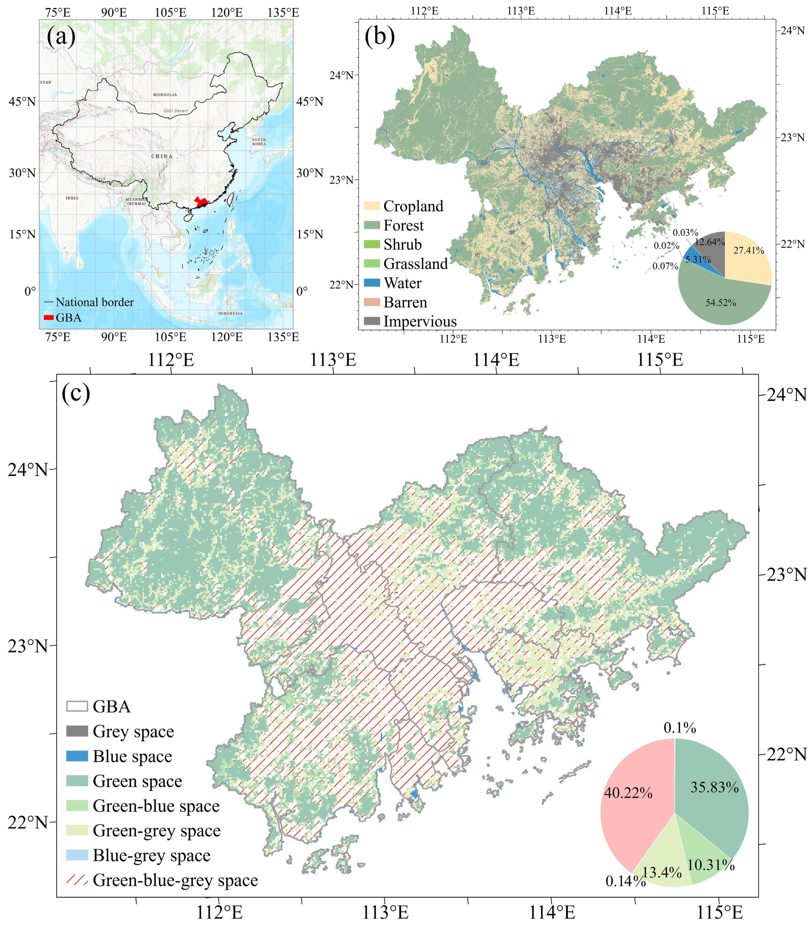
2.1. Study Area

The Guangdong-Hong Kong-Macao Greater Bay Area (GBA) is situated in southern China and has a subtropical monsoon climate, with an average annual temperature of 22 °C. The GBA includes Hong Kong, Macao, Guangzhou, Shenzhen, Zhuhai, Foshan, Huizhou, Dongguan, Zhongshan, Jiangmen, and Zhaoqing. The GBA has predominantly flat terrain, with plains covering 66.7% of its area. Hills, plateaus, and residual hills comprise about 20% of the area, while mountains cover just 3%. Located in the Pearl River Delta, the GBA has 102 major rivers stretching over 1700 km, forming a complex network of waterways. The GBA has undergone rapid urbanization since the 1980s. Urban expansion, fueled by high population density and extensive transportation networks, has intensified the urban heat island effect [11,66,67].

2.2. Data Sources and Preprocessing

2.2.1. Land Cover Data

In recent decades, rapid economic growth and population expansion in the GBA have driven significant changes in land cover. This study used the 30 m Annual China Land Cover Dataset (CLCD, available at http://doi.org/10.5281/zenodo.4417809) in 2020 to extract water bodies as blue spaces and impervious surfaces as grey spaces (Figure 1b). We then used Landsat 8 data to calculate the monthly Normalized Difference Vegetation Index (NDVI) on the Google Earth Engine (GEE) platform and categorized forests, shrubs, grasslands, and cropland as green spaces (Supplementary Figure S1). A 1 km spatial resolution grid was created to calculate the coverage of green, blue, and grey spaces within each cell. Based on these coverages, the GBA was classified into various spatial regions (Table 1). To explore the relationships between the blue, green, and grey spaces, we defined their combinations as the main study area (Figure 1c). In this study, green space, blue space, and grey space refer to the respective components within the green–blue–grey spaces (GBGSs).

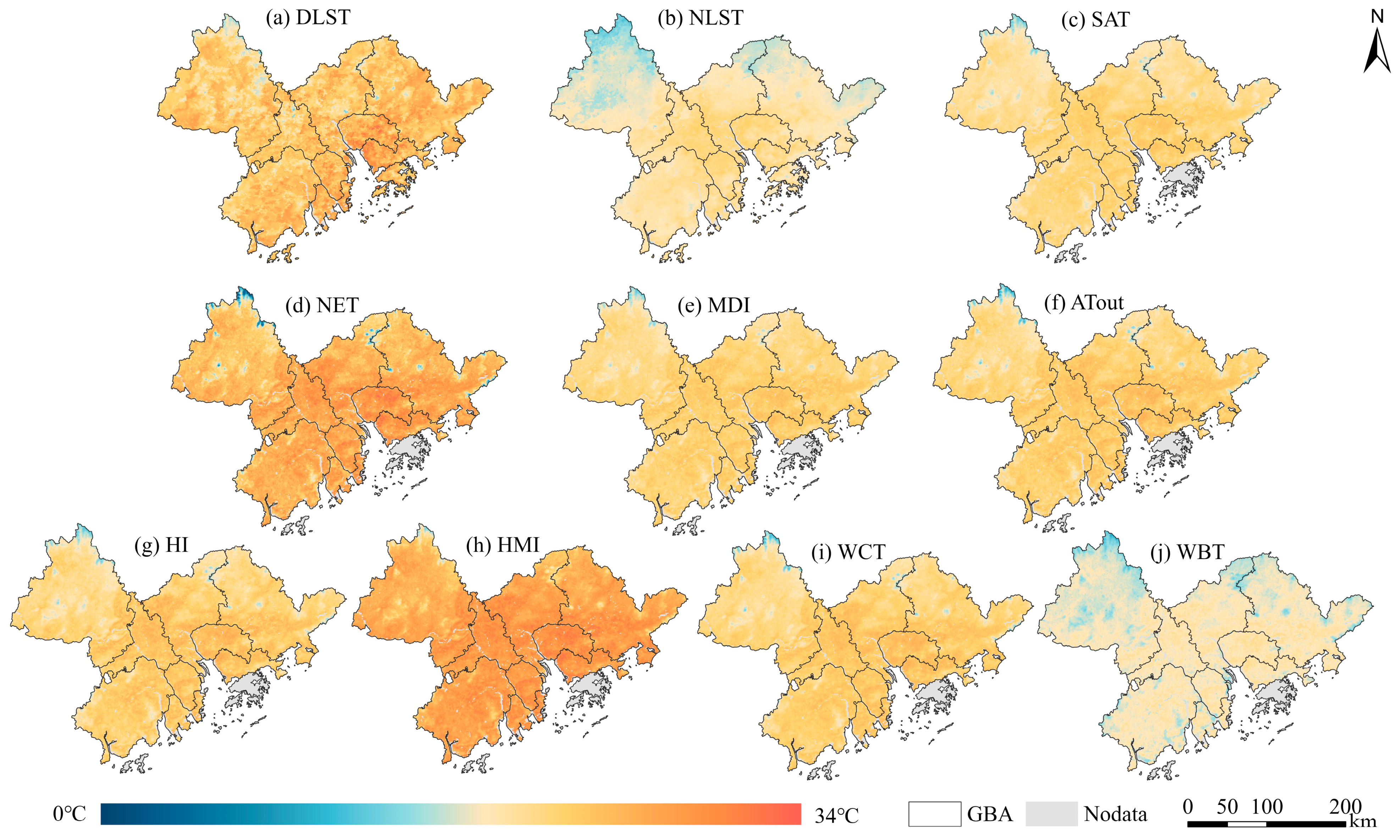
2.2.2. Indicators of Urban Thermal Environments

Urban thermal environment indicators include surface temperature, near-surface air temperature, and various human heat indices (Table 2). Surface and near-surface air temperatures represent surface urban thermal environments (STE), while human thermal indices reflect Perceptual Urban Thermal Environments (PTEs). Daytime land surface temperature (DLST) and nighttime land surface temperature (NLST) are widely used in urban heat environment studies due to their ability to effectively reflect the extent and intensity of UHI [64,68,69]. Zhang generated a 1 km human thermal index dataset (HiTIC-Monthly) for China from 2003 to 2020 based on machine learning and various factors [70]. This dataset characterizes human-perceived temperatures, including outdoor shaded temperature (ATout), net effective temperature (NET), heat stress index (HMI), heat index (HI), wind chill temperature (WCT), and wet-bulb temperature (WBT), among others. We extracted all thermal indices for the GBA region and calculated the annual mean for each index within the grid.

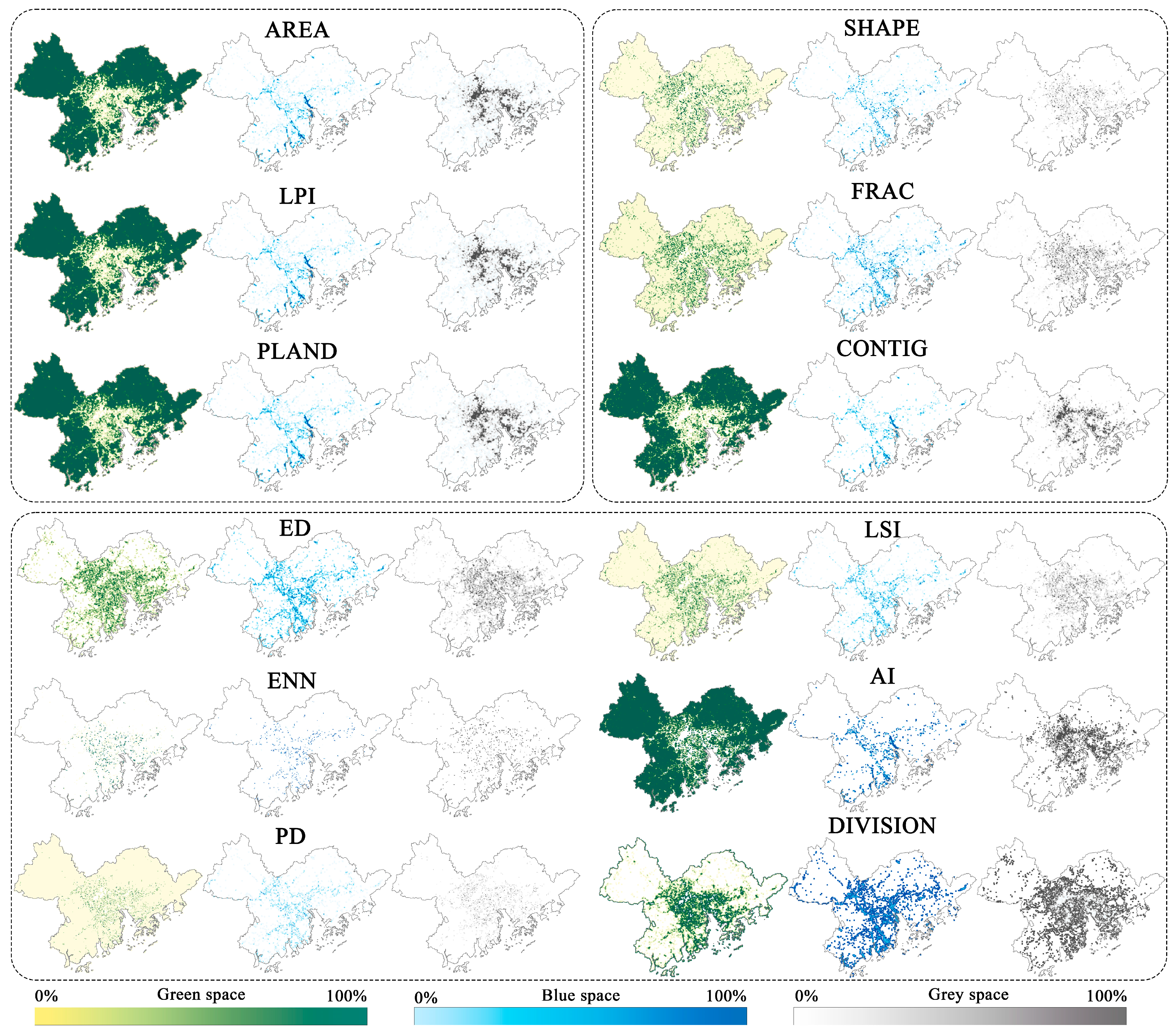
2.2.3. Indicators of Urban Space Coverage and Landscape

To investigate the impact of each index on the thermal environment, we used 13 indicators, including coverage and landscape of GBGS (Table 3). Coverage is calculated based on the area of spaces within each grid. The composition, configuration, and spatial complexity of landscape elements define the landscape pattern. Landscape indices (Area, Shape, and Aggregation) are calculated at the patch scale using Fragstats within a 1 km moving window. These indices were standardized to a range of 0 to 100, expressed as percentages.

2.3. Methods

2.3.1. Methodology for Analyzing the Relationship Between USCL and UTE

We used Pearson’s correlation coefficient, OPGD (Optimal Proportional Gradient Difference), and XGBoost (Extreme Gradient Boosting) to explore the relationship between USCL and UTE. We then calculated the CE of blue and green spaces and the WE of grey spaces to summarize the optimal spatial coverage and explored spatial patterns under different combination scenarios (Figure 2).
This study uses Pearson correlation coefficients, XGBoost, and the Optimal Parameters-based Geographical Detector (OPGD) to investigate the relationship between USCL and UTE. Pearson’s correlation coefficient is a statistical measure that quantifies the linear relationship between two variables, ranging from −1 to 1. A value of 1 indicates a perfect positive relationship, −1 is a perfect negative relationship, and 0 is no linear relationship. It is commonly used to analyze the relationship between land use types and urban thermal environments [37,71]. XGBoost (Extreme Gradient Boosting) is a machine learning algorithm based on gradient boosting, particularly effective for processing remote sensing data with limited sample sizes [71,72]. XGBoost evaluates the contribution of independent variables to the dependent variable by learning from sample data and variable features. This makes it valuable for explaining how spatial layout differences influence variations in the urban thermal environment. The Optimal Parameters-based Geographical Detector (OPGD) is a set of statistical methods designed to detect spatial heterogeneity and identify underlying driving factors [73]. It is widely used to distinguish, detect, and analyze interactions among driving factors [74,75,76,77].

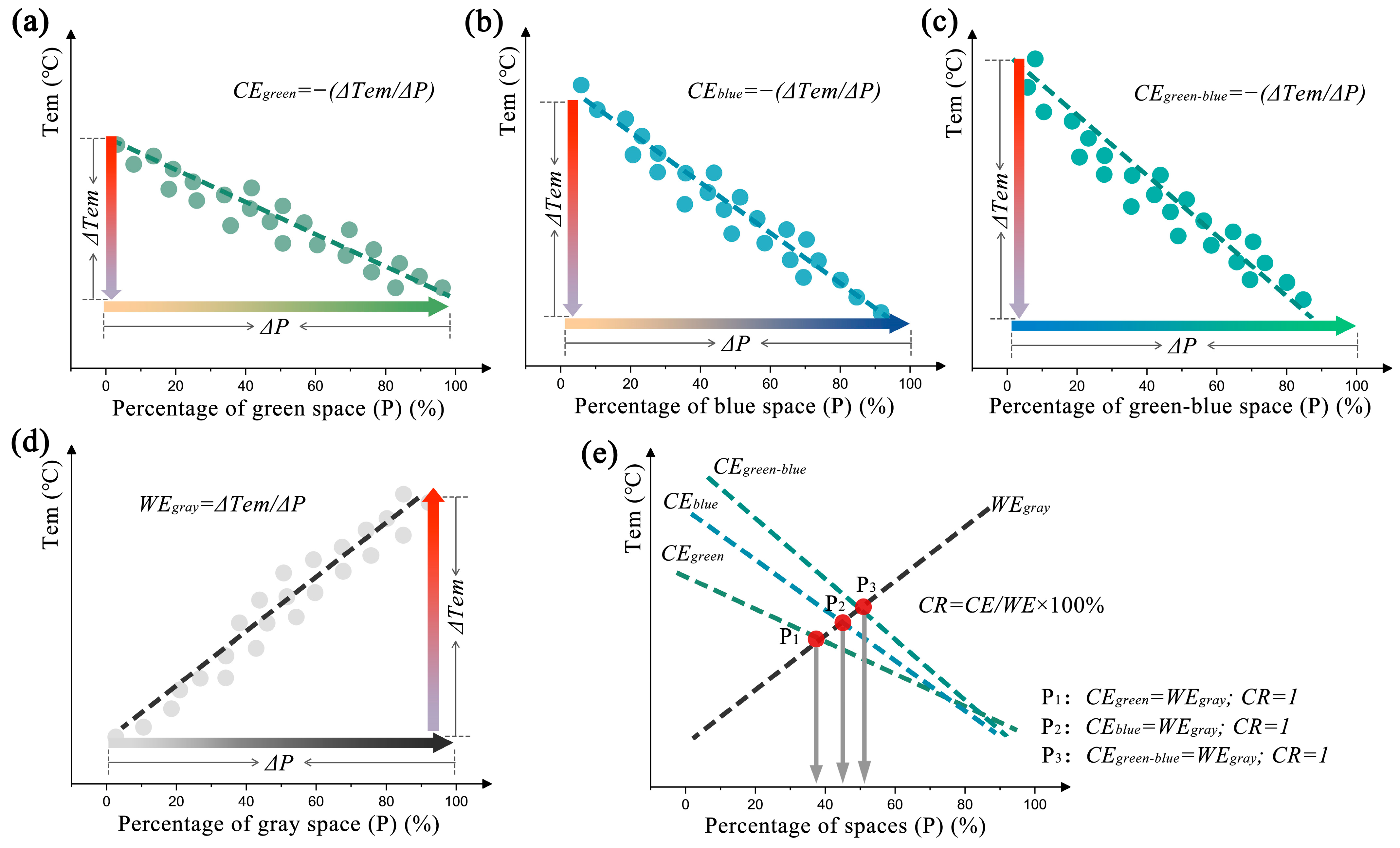
2.3.2. Cooling Efficiency and Warming Efficiency of USCL

Green and blue spaces significantly cool urban surface temperatures, while grey space tends to have a warming effect. Cooling efficiency (CE) refers to the temperature reduction resulting from a one-unit increase in cooling space patterns (e.g., a 1% increase in green space coverage). Warming efficiency (WE) refers to the temperature increase associated with a one-unit increase in warming space patterns (e.g., a 1% increase in grey space coverage). CE is calculated using the negative value of the coefficient from the Ordinary Least Squares (OLS) regression between green or blue space pattern indices and UTE indices (Figure 3a–c) (Equation (1)). WE is calculated using the coefficient from the regression between grey space pattern indices and UTE indices (Figure 3d) (Equation (2)).
C E i , j = Δ T e m i / Δ P j
W E i , j = Δ T e m i / Δ P j
where C E i , j represents the cooling efficiency, measured in °C/%; W E i , j represents the warming efficiency, measured in °C/%; Δ T e m represents the temperature difference between different grids; Δ P represents the difference in spatial pattern indices between different grids; i refers to the urban heat index (Table 2); j refers to the urban spatial pattern index (Table 3).
Cooling-to-Warming Ratio (CR) is defined as the ratio of the temperature increase from 1% additional grey space that can be offset by 1% of green or blue space. It is calculated as the ratio between the cooling efficiency of cooling spaces and the warming efficiency of warming spaces (Equation (3)).
C R i , j = C E i , j / W E i , j
where C R is the ratio of C E and W E ; i refers to the urban heat index (Table 1); j refers to the urban spatial pattern index (Table 2). When C R < 1, it means W E > C E , indicating that a 1% increase in cooling space cannot fully offset the warming effect of a 1% increase in warming space. When C R > 1, it means C E > W E , meaning that a 1% increase in cooling space can fully offset the warming effect of a 1% increase in warming space. When C R = 1, C E equals W E . Therefore, we can determine the intersection points between the fitted CE and WE equations (Figure 3e). P1 is the intersection of the green space fitting equation and the grey space equation, P2 is the intersection of the blue space fitting equation and the grey space equation, and P3 is where the combined green and blue space fitting equation intersects with the grey space equation. The x-values corresponding to P1, P2, and P3 represent spatial indices (e.g., space coverage), expressed as percentages. To maximize cooling efficiency and minimize warming efficiency, the coverage of cooling spaces should be at least P1, P2, or P3, while the maximum coverage of warming spaces should not exceed P1, P2, or P3. (For example, in green–grey spaces, the minimum green space coverage is P1 (%), and the maximum grey space coverage is P1 (%).)

3. Results

3.1. Spatial Distribution of Urban Spaces and Thermal Environments

The GBA is predominantly covered by forest, with impervious surfaces primarily concentrated in the core urban areas (Figure 1b). Rivers, lakes, and reservoirs form a network that is widely distributed across the GBA. Forests make up the largest share of land cover in the GBA (54.52%), primarily found in the northwest mountainous areas and the northern ecological development zone. Cropland ranks second (27.41%), mainly located in the eastern and western regions. A total of 12% of the impervious surfaces in the GBA are concentrated in the core urban area, where the Xijiang, Beijiang, and Dongjiang rivers converge. This region has a relatively high proportion of water. In terms of urban regions classified by grid coverage, GBGS is mainly concentrated in the core urban clusters of the Pearl River Delta (Figure 1c). The average proportion of green space in each grid is 64.16%, while blue space makes up 11.23%, and grey space accounts for 21.1%. Green–grey space ranks second in proportion, after composite space and pure green space, in the GBA. In this category, green space makes up 76.52%, while grey space accounts for 21.63%. Green–Blue space also has a relatively high proportion, with green space (86.67%) being 12 times greater than the average water share (7.16%). In blue–grey space, the proportion of blue space (32.53%) is double that of grey space (14.6%). These variations in area proportions result in different landscape patterns of green, blue, and grey spaces in the GBA (Figure 4).
The UTE in the GBA shows significant variation in layout (Figure 5). High-temperature areas are primarily concentrated in core cities of the Pearl River Delta, including Guangzhou, Shenzhen, Dongguan, Foshan, Hong Kong, and Macau. Sub-high-temperature zones are located in the urban areas of Jiangmen, Zhuhai, Huizhou, and Zhaoqing. Cool zones are concentrated in the mountainous regions of northern and eastern GBA. Specifically, while the spatial distributions of STE and PTE are similar, there are differences in temperature levels (Table 4). The 2020 annual average temperatures in the GBA were 23.04 °C for DLST, 18.76 °C for NLST, and 21.16 °C for SAT. The NET was 16.21 °C, while the ATout is 22.07 °C. The HI, HMI, and WCT were relatively high, with annual averages of 22.23 °C, 27.07 °C, and 22.17 °C, respectively. The average WBT was 18.32 °C, and the average discomfort index is 21.79 °C. Overall, the perceived temperature is slightly higher than LST and SAT.
Thermal differences also exist across different zones (Figure 6). Grids containing green space (such as green and green–blue) show a wider range between STE and PTE, with average temperatures lower than the overall regional average (Table 4). In contrast, grids with grey space (such as grey, green–grey, and blue–grey) have higher average temperatures than the regional average.

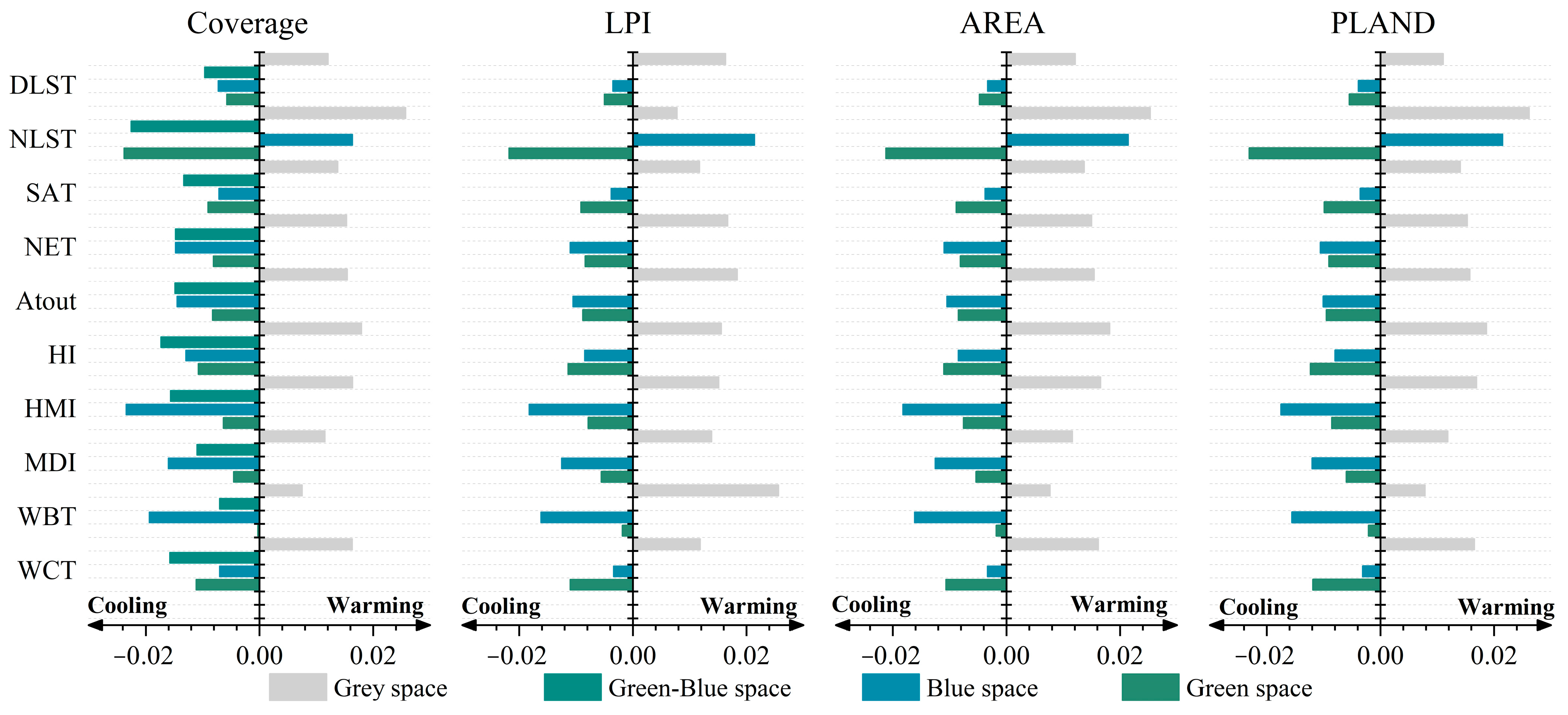
3.2. The Coverage and Landscape of Urban Spaces Significantly Affect the Thermal Environments

The Pearson correlation coefficient indicates a significant correlation between the coverage and landscape of urban spaces and the UTE (Figure 7a). The correlation between UTE and indices related to spatial perimeter and area is stronger than with those related to spatial shape and aggregation. Most green space indices are significantly negatively correlated with both perceived STE and PTE. ED, DIVISION, and ENN exhibit a significant positive correlation with the UTE. This suggests that green spaces have a substantial cooling effect on the regional thermal environment. Due to their strong heat absorption and limited heat dissipation, the coverage and landscape of grey spaces are significantly positively correlated with urban thermal indices. XGBoost contribution results show that grey space coverage has the greatest impact on UTE, followed by the PLAND and PD of grey spaces, the ED of green spaces, and the CONTIG and LPI of grey spaces (Figure 7b). Blue space indices are significantly negatively correlated with DLST and perceived temperature but significantly positively correlated with NLST. This suggests that larger blue spaces or more rational landscape distribution leads to lower daytime land surface temperatures and perceived temperatures. However, water’s slower heat dissipation results in higher temperatures at night. Interaction analysis results show that all USCL indices either exhibit a two-factor or nonlinear enhancement effect on UTE indices (Figure 7c). This indicates that the combined impact of urban space coverage and landscape on the urban thermal environment is greater than optimizing individual factors alone. Among them, the combination of green space edge density and grey space coverage has the greatest impact on DLST, SAT, NET, MDI, ATout, HI, HMI, and WBT. Conversely, blue space coverage and grey space AREA have the greatest impact on NLST and WCT.

3.3. Cooling and Warming Efficiency in Different Urban Spaces Coverage

Urban green spaces, blue spaces, and blue–green spaces have varying cooling efficiencies on the UTE, whereas grey spaces exhibit a significant warming effect (Figure 8). Coverage represents the cooling or warming effect resulting from a 1% increase in each space type within each grid. Blue spaces absorb significant solar radiation during the day and release it slowly at night, causing a warming effect on NLST with a WE of 0.1634 °C/%. However, blue spaces exert a cooling effect on other temperature indices, with an average CE of 0.0136 °C/%, while green spaces have a lower average CE of 0.0088 °C/% on the UTE. The CE difference between blue and green spaces is small for PTE, but blue spaces are more effective in cooling than green spaces for STE. Additionally, the average CE of blue–green spaces on the UTE is 0.1422 °C/%, indicating that the cooling effect of the combined blue and green space distribution is greater than that of either space type alone. In contrast, the average WE of grey spaces on the UTE is 0.1519 °C/%, higher than the CE of blue spaces, green spaces, and blue–green spaces. This means that a 1% increase in grey space requires more blue–green spaces to counterbalance the warming effect. LPI, AREA, and PLAND characterize the cooling and warming efficiencies of each 1% increase in maximum patch share, patch area, and patch percentage for different space types. Consistent with the coverage calculations, LPI, AREA, and PLAND of blue and green spaces contribute to cooling the urban thermal environment, whereas grey spaces intensify warming. However, the WE and CE do not fully offset each other.
CR (Cooling-to-Warming Ratio) measures the ability of blue and green spaces to mitigate the warming effect of grey spaces (Figure 9a). A 1% increase in green spaces can offset only 48.17% of the temperature rise caused by a corresponding increase in grey spaces for DLST, while a 1% increase in blue spaces offsets 60.4%, and in blue–green spaces, 80.26%. For SAT, a 1% increase in green spaces or blue spaces can offset 65.99% and 52.14% of the warming effect of grey spaces, respectively, while a 1% increase in blue–green spaces can offset 97.01%. For PTE, a 1% increase in blue–green spaces can offset more than 95% of the warming effect. For WBT, green spaces have a low cooling efficiency, while blue spaces exhibit a highly significant cooling effect. Green spaces have a higher CE for STE than for PTE, whereas blue spaces have a stronger cooling effect for PTE than for STE. Furthermore, the results highlight that relying solely on green spaces to counteract the warming effect of impermeable surfaces may be less effective. Increasing the area of blue spaces and improving the layout of blue–green combined spaces is the most effective approach to mitigating the urban heat island effect.
The intersection points of the fitting lines for different spaces indicate the balance between the CE and WE of blue, green, and grey spaces (from Figure 9b–k). To the left of the intersection, the CE is greater than the WE; to the right, the WE exceeds the CE. The spatial proportions at the intersection correspond to the maximum coverage of grey spaces and the minimum coverage of blue or green spaces. The warming effect (WE) surpasses the cooling effect (CE) when green space falls below or grey space exceeds a certain threshold, with similar patterns observed for blue space and combined blue–green space. Specifically, for DLST, the threshold is 35.56% for green space, 17.37% for blue space, and 45.45% for blue–green space (Figure 9b). For NLST, these values are 42.6%, 38%, and 46.73% (Figure 9c), while for SAT, they are 40%, 18.1%, and 49.63% (Figure 9d). NET follows with thresholds of 38.26%, 16%, and 49.67% (Figure 9e), and MDI with 32.94%, 14.64%, and 47.83% (Figure 9f). Similarly, for HMI, the thresholds are 35.91%, 15.38%, and 49.37% (Figure 9g), for HI they are 38.62%, 16.77%, and 49.71% (Figure 9h), and for ATout they are 39.13%, 16.33%, and 50% (Figure 9i). WBT exhibits two sets of thresholds: 25.35%, 13.85%, and 50.71%, as well as 41.11%, 18.7%, and 49.69% (Figure 9j). These thresholds indicate the critical balance points where urban thermal conditions shift from a cooling-dominated to a warming-dominated state.
To balance cooling and warming across all temperature indices, a 1 km2 grid should include at least 37% green space, 18% blue space, or a combined 49% of both (Figure 9l). These proportions counteract the warming effect of an equivalent grey space area. For PTE cooling, an even higher proportion is required. For STE, the mean P1 value is 39.38%, indicating that when green space covers less than 40%, warming outweighs cooling, making the area predominantly warm. For PTE, the mean P1 value is 35.9%, suggesting that when green space falls below 36%, the warming effect intensifies. Similarly, the mean P2 values for STE and PTE are 24.49% and 15.95%, while the mean P3 values are 47.27% and 49.57%, respectively. This suggests that, for STE, at least 24.49% blue space and 47.27% combined blue–green space are needed to counteract grey space warming and enhance cooling. For PTE, at least 15.95% blue space and 49.56% combined blue–green space are required.

3.4. Optimal Configuration of Urban Space Coverage and Landscape

To ensure the cooling effect exceeds the warming effect, we combined the impacts of green, blue, and blue–green spaces on all temperature indices, STE, and PTE. The average coverage values calculated were 37.64% for green space, 20.22% for blue space, and 48.41% for blue–green combined space. To simplify the spatial combinations, we converted the coverage values into integers and established three scenarios: Plan A: Green space is dominant, with each grid containing at least 40% green space, and the grey space threshold equals that of green space, i.e., no more than 40%, resulting in 14 combinations (Figure 10a). Plan B: Blue space is dominant, with each grid containing at least 20% blue space, and the grey space threshold equals that of blue space, i.e., no more than 20%, resulting in 13 combinations (Figure 10b). Plan C: Blue–green combined space is dominant, with each grid containing at least 50% blue–green space, and the grey space threshold equals that of the blue–green combined space, i.e., no more than 50%, resulting in 20 combinations (Figure 10c). After removing duplicates, 30 unique combinations were identified (Figure 10d). We explored the optimal coverage and landscape combinations of urban blue, green, and grey spaces by comparing the cooling (CE) and warming (WE) effects across these 30 combinations.
Different coverages and landscape configurations of grey spaces lead to varying warming effects (Figure 11). When grey space covers less than 10%, the warming effect of FRAC is highest (WE = 0.062), while CONTIG, AI, and DIVISION show cooling effects. Therefore, lower connectivity and aggregation, combined with higher fragmentation, can reduce the ability of grey spaces to warm. However, as grey space coverage increases to 20%, the WE of FRAC significantly decreases, while the WE of DIVISION significantly increases. CONTIG and AI continues to show a cooling effect. Higher fragmentation, along with lower connectivity and aggregation, enhances the warming effect. As grey space forms larger, contiguous patches, its heat storage capacity increases, resulting in a significant warming effect. When grey space coverage is below 30%, the warming effect (WE) of SHAPE, LSI, ED, and PD remains around 0.01 °C/%. However, when coverage is between 30% and 50%, the WE of these indices ranges from −0.008 to 0.004 °C/%. This suggests that moderate grey space coverage, combined with optimized landscape characteristics, helps reduce local temperatures. ENN reaches an inflection point at 30% grey space coverage. When coverage is below 30%, increasing patch distance significantly raises temperatures. When coverage exceeds 30%, increasing patch distance significantly cools the area.
The CE of blue and green spaces varies with different landscape configurations under the same coverage of grey spaces (Figure 12). In a grid with 10% grey spaces, there are eight blue–green space scenarios (Figure 12a). When green space coverage is less than 40%, shape indices (SHAPE, FRAC) show higher CE. However, when green space exceeds 40%, the CE of shape indices becomes negative. This suggests that more complex green space shapes contribute to warming. Aggregation indices, in contrast, consistently show a slight cooling or warming effect. When blue space coverage is between 50% and 60%, FRAC shows relatively high CE, while DIVISION and ENN have a warming effect. Therefore, large, aggregated, and complex water is beneficial for cooling. In a grid with 20% grey spaces, there are seven blue–green space scenarios (Figure 12b). For green space, the coverage range of 30% to 40% marks the inflection points where shape and aggregation indices shift from cooling to warming. For blue space, FRAC shows the highest CE, but as coverage decreases, cooling efficiency diminishes. In a grid with 30% grey spaces, there are six blue–green space scenarios (Figure 12c). In these scenarios, the contribution of green space shape and aggregation to cooling is minimal. In contrast, blue spaces with more complex boundaries and higher fragmentation show more significant cooling benefits. In a grid with 40% grey spaces, there are five blue–green space scenarios (Figure 12d). When green space coverage is greater than 10% but less than 40%, the CE of shape indices is high, particularly FRAC and ENN. However, it shifts to a warming effect once coverage reaches 40%. For blue space, when coverage is between 40% and 50%, CE is relatively high across all indices, but ENN and DIVISION show warming effects. As blue space coverage decreases, the influence of shape and aggregation indices on temperature gradually weakens. In a grid with 50% grey spaces, there are four blue–green space scenarios (Figure 12c). When green space coverage is 20%, both shape and aggregation indices show relatively high CE. In addition to warming NLST, 30% blue space demonstrates a significant cooling effect on the overall urban thermal environment.

4. Discussion

4.1. Perceived Temperature and Its Role in Urban Thermal Environment

Human well-being is influenced by various environmental factors, one of which is the thermal state of the environment [78]. Unlike traditional studies that focus on the cooling efficiency of blue–green spaces, this study explores the effects of blue–green and grey spaces on perceived temperature and their respective cooling and warming efficiencies from a subjective perception standpoint. By integrating both physical and perceived thermal environments, this study explores optimal spatial proportions and layout strategies. Its goal is to reduce land surface and near-surface air temperatures while also considering residents’ comfort and well-being. Global warming, coupled with the urban heat island effect, has led to more frequent regional heatwaves and extreme heat events. This trend is expected to worsen, posing a significant threat to human physical and mental health [6,79,80]. However, most studies on urban heat environments have focused primarily on land surface or canopy height air temperatures [12,81], while human-perceived temperature—an intermediate measure between the physical thermal environment and human perception—requires more attention [78,80,82,83,84]. Spatial quantification of both physical and perceived thermal environments shows that human-perceived temperatures in the GBA differ from physical temperatures, suggesting that factors like humidity and wind speed influence how individuals experience temperature. Both are also influenced by urban land use patterns and spatial configurations [52,82]. Areas with a high proportion of blue–green spaces have lower physical and perceived temperatures, while areas dominated by grey spaces exhibit higher temperatures. This finding aligns with studies by Ferdinando Salata and Coccolo [79,85]. Furthermore, Pigliautile et al. integrated human physiological parameters into urban canopy models, highlighting that green space cools perceived temperature by reducing land surface temperature [82]. In addition to cooling benefits, green spaces and water bodies also promote mental well-being and have been shown to provide stronger cooling effects for socially vulnerable populations [59,86]. Therefore, a human-centered integrated research framework enables the quantitative analysis of the spatiotemporal evolution of the objective thermal environment. It also examines the impact of urban spatial layout on perceived temperature, offering new insights for future landscape optimization.

4.2. Optimal Combination of Green Blue and Grey Space for Urban Thermal Environment Cooling

Controlling urban expansion is critical to mitigating the urban heat island effect. However, replacing natural vegetation and water bodies with impervious surfaces is often inevitable during urban development. This study analyzes the proportions and spatial arrangements of green, blue, and grey spaces to assess their cooling (CE) and warming (WE) efficiencies. Impervious surfaces contribute to warming due to their high heat capacity and low reflectivity [43]. In the GBA, this study finds that when grey spaces coverage within a 1 km2 area is lower than 40%, the cooling efficiency of blue–green spaces outweighs the warming efficiency. Thus, controlling the proportion of impervious surfaces within this range is advisable. However, Gao et al. recommend a building coverage ratio of no more than 62% in Wuhan, Hubei Province [87]. Moreover, moderately dispersed, polycentric urban clusters can help reduce Surface Heat Urban Intensity (SHUI) [88]. Thus, future urban planning should prioritize controlling impervious surface proportions and increasing patch fragmentation [62,88].
However, thresholds for these factors vary across regions. Regional variations should be accounted for to effectively mitigate urban heat island effects and optimize thermal green spaces, which reduce radiative and air temperatures through shading and evaporation [41,89]. In the GBA, research shows that at least 35% vegetation coverage is needed for cooling efficiency to exceed warming efficiency. This threshold underscores the need to maintain and expand green spaces in urban areas to mitigate urban heat island effects and improve urban quality. The presence of water helps regulate the thermal environment by absorbing and storing heat during the day and releasing it gradually at night, thereby stabilizing temperature fluctuations and reducing the overall heat load in urban areas [56,90,91]. Integrating more water features in urban planning is a promising strategy for mitigating urban heat island effects, enhancing thermal comfort, and promoting sustainability to improve urban resilience [46,51,85]. Consistent with findings by Sameh Kotb Abd-Elmabod [51], Chen [36], Cai [92], and Mitchell [93], this study shows that water bodies have higher cooling efficiency than green spaces.
Additionally, the cooling effect of combined blue–green spaces is significantly greater than that of either green or blue space alone. This highlights the importance of incorporating both blue and green spaces in urban planning to optimize cooling and enhance resilience. Future urban planning should prioritize increasing water proportions, followed by expanding tree planting. In fixed-area scenarios, the shape and layout of blue–green spaces significantly influence heating and cooling effects. Research suggests that increasing building fragmentation and enhancing connectivity between green and blue spaces can improve cooling efficiency [37]. Simple-shaped blue–green spaces are more effective for cooling, as they facilitate efficient heat dissipation and better thermal regulation [94]. This approach fosters more effective and resilient urban landscapes [95]. Some scholars stress the importance of increasing blue–green space patches to create a more fragmented landscape [58,88]. This perspective is shaped by variations in urban development and climate across regions [56,96]. In the GBA, a balanced level of complexity and fragmentation in the urban landscape can mitigate the urban heat island effect. Although the conclusions regarding the spatial layout of blue, green, and grey spaces in the GBA may not be applicable to cities with different climates, the methods of using CE and WE to offset are transferable and can be applied to regional analyses of other cities to determine spatial coverage thresholds and optimal configurations.

4.3. Limitations of the Study

This study focuses solely on the planar combination of grey, green, and blue spaces in urban spatial configurations. In practice, blue and green space proportions can be increased through spatial layering, such as green roofs, which are an effective cooling strategy [97,98]. Factors like building height and ventilation corridor design are crucial for improving airflow and mitigating urban heat islands. Wu et al. found that 2D morphological indicators have a greater impact than 3D indicators [39]. Thus, this study examines optimal spatial layouts at the two-dimensional level. While most studies emphasize the cooling effect of vegetation on urban thermal environments, they typically focus on urban trees or shrubs as green spaces. In this study, forests, shrubs, grasslands, and croplands identified through NDVI calculations are classified as green spaces. However, the study does not consider that some vegetation in high-latitude cities is seasonal and provides cooling benefits only during the growing season. Further research is needed to synthesize qualitative and quantitative perspectives to explore urban spatial configurations in temperate and cold regions, as well as the differences between urban centers and rural areas. In terms of data usage, we downplay the temporal characteristics of the data to focus on the spatial impact on temperature. The different spatial combinations of green, blue, and grey spaces may exhibit seasonal variations or changes due to extreme weather events, which warrants further investigation.

5. Conclusions

This study analyzed the spatial distribution pattern of physical and perceived thermal environments in the GBA. Moreover, the cooling and warming efficiencies were calculated based on the coverage and landscape of GBGS to identify optimal spatial configurations. The main conclusions are as follows:
  • There is a significant spatial consistency between the physical and perceived thermal environments in the GBA. Humidity and wind speed contribute to discrepancies between perceived temperature and physical environmental temperature. Perceived temperatures, including sultry and humid-heat temperatures, are lower than daytime land surface temperatures but higher than near-surface air temperatures. Discomfort temperatures exceed all temperature indices by 4 to 10 °C. Both thermal environments, however, are influenced by land use patterns and landscape configurations;
  • Green and blue spaces offer substantial cooling benefits to both physical and perceived urban thermal environments, while grey spaces contribute to warming. While blue spaces can warm nighttime land surface temperatures, their overall cooling effect on the urban thermal environment remains significant. The cooling efficiency (CE) of combined blue–green spaces (average CE of 0.014 °C/%) exceeds that of green spaces alone (average CE of 0.009 °C/%) or blue spaces alone (average CE of 0.013 °C/%);
  • Spatial coverage significantly impacts the regional thermal environment. Urban planning should limit the expansion of grey spaces, keeping their proportion below 30–40% per square kilometer. Green spaces should make up at least 35%, while blue spaces should comprise 15–25%. On average, a 1% increase in green space can offset 54% of the warming caused by an equivalent increase in grey space, while the same increase in blue space can offset 87%. A combination of blue and green spaces can mitigate up to 95% of the warming effect;
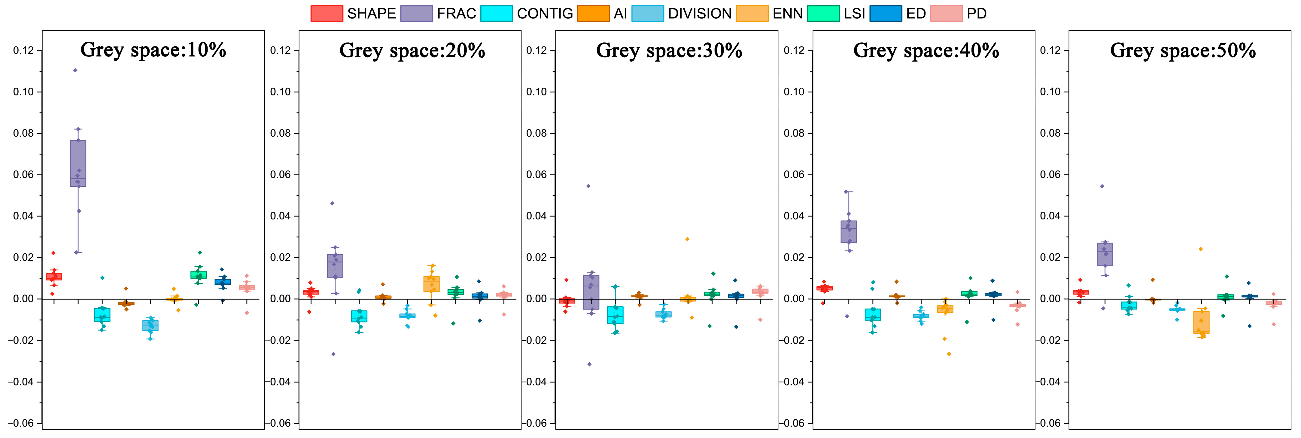
  • The shapes and degrees of aggregation of GBGS also influence regional temperatures. In grids with low grey space proportions (10–20%), increasing blue space and simplifying the shapes of green spaces improve overall cooling efficiency. When the grey space proportion is moderate (30–40%), increasing the boundary complexity of blue spaces should be prioritized. In grids with a high grey space proportion (50%), blue space should be maintained at approximately 30%, while optimizing green space aggregation and shape, and enhancing cooling capacity through a green space network.
These findings emphasized the critical role of GBGS in mitigation of urban thermal environment. Urban planning should regulate the proportion of grey spaces and optimize the configuration of blue–green spaces to mitigate urban thermal stress and enhance cooling efficiency. Additionally, integrating human thermal comfort considerations by optimizing spatial morphology, improving ventilation, and increasing blue–green space connectivity can enhance urban livability.

Supplementary Materials

The following supporting information can be downloaded at https://www.mdpi.com/article/10.3390/land14030645/s1. Figure S1: The monthly NDVI values for forests, croplands, shrublands, and grasslands in the GBA region; Figure S2: The ordinary least squares regression fitting results of the coverage of green, blue, blue-green combined spaces, and grey space with temperature indices; Table S1: The cooling efficiency and warming efficiency offset ratios and areas of different spaces; Table S2: 30 unique combinations and the number of grids corresponding to different types; Table S3–S32: The cooling efficiency/warming efficiency of green, blue and grey spaces landscape patterns with different coverage ratio.

Author Contributions

W.Z.: Conceptualization, Methodology, Visualization, Writing—original draft and Writing—review and editing. K.Y.: Conceptualization, Supervision. S.Z.: Conceptualization, Visualization, Supervision and Writing—review and editing. C.B.: Methodology and Writing—original draft. J.L. and X.Y.: Conceptualization. Y.R.: Visualization. Y.M.: Methodology. All authors have read and agreed to the published version of the manuscript.

Funding

This work was supported by the National Natural Science Foundation of China (42071381 and 42471469).

Data Availability Statement

The original contributions presented in this study are included in the article; further inquiries can be directed to the corresponding authors.

Conflicts of Interest

The authors declare no conflicts of interest.

Abbreviations

The following abbreviations are used in this manuscript:
GBGSGreen Blue Grey Spaces
LSTLand Surface Temperature
SATSurface Air Temperature
STESurface Urban Thermal Environments
PTEPerceptual Urban Thermal Environments
UTEUrban Thermal Environments
UHIUrban Heat Island
UCIUrban Cooling Island
GBAGuangdong-Hong Kong-Macao Greater Bay Area
USCLUrban Space Coverage and Landscape
CECooling Efficiency
WEWarming Efficiency
CRCooling-to-Warming Ratio
TVoEThreshold Values of Efficiency
CGCooling Gradient
CICooling Intensity
ASArtificial Surfaces
PETPhysiological Equivalent Temperature
UTCIUniversal Thermal Climate Index
DLSTDay Land Surface Temperature
NLSTNight Land Surface Temperature
NETNet Effective Temperature
ETEffective Temperature
ATApparent Temperature
HIHeat Index
HMIHumidex
DIDiscomfort Index
MDIModified Discomfort Index
WCTWind Chill Temperature
WBTWet-Bulb Temperature

References

  1. Bai, Y.; Wang, W.; Liu, M.; Xiong, X.; Li, S. Impact of urban greenspace on the urban thermal environment: A case study of Shenzhen, China. Sustain. Cities Soc. 2024, 112, 105591. [Google Scholar] [CrossRef]
  2. Massaro, E.; Schifanella, R.; Piccardo, M.; Caporaso, L.; Taubenbock, H.; Cescatti, A.; Duveiller, G. Spatially-optimized urban greening for reduction of population exposure to land surface temperature extremes. Nat. Commun. 2023, 14, 2903. [Google Scholar] [CrossRef]
  3. Raymond, C.; Matthews, T.; Horton, R.M. The emergence of heat and humidity too severe for human tolerance. Sci. Adv. 2020, 6, eaaw1838. [Google Scholar] [CrossRef] [PubMed]
  4. Guo, Y.; Gasparrini, A.; Armstrong, B.G.; Tawatsupa, B.; Tobias, A.; Lavigne, E.; Coelho, M.; Pan, X.; Kim, H.; Hashizume, M.; et al. Heat Wave and Mortality: A Multicountry, Multicommunity Study. Environ. Health Perspect. 2017, 125, 087006. [Google Scholar] [CrossRef]
  5. Tong, S.; Prior, J.; McGregor, G.; Shi, X.; Kinney, P. Urban heat: An increasing threat to global health. BMJ 2021, 375, n2467. [Google Scholar] [CrossRef]
  6. Estoque, R.C.; Ooba, M.; Seposo, X.T.; Togawa, T.; Hijioka, Y.; Takahashi, K.; Nakamura, S. Heat health risk assessment in Philippine cities using remotely sensed data and social-ecological indicators. Nat. Commun. 2020, 11, 1581. [Google Scholar] [CrossRef]
  7. Zhang, X.; Chen, F.; Chen, Z. Heatwave and mental health. J. Environ. Manag. 2023, 332, 117385. [Google Scholar] [CrossRef]
  8. Fouillet, A.; Rey, G.; Laurent, F.; Pavillon, G.; Bellec, S.; Guihenneuc-Jouyaux, C.; Clavel, J.; Jougla, E.; Hemon, D. Excess mortality related to the August 2003 heat wave in France. Int. Arch. Occup. Environ. Health 2006, 80, 16–24. [Google Scholar] [CrossRef]
  9. Yang, J.; Bao, L.; Dong, S.; Qiu, Y.; Gao, J.; Zou, S.; Tao, R.; Fan, X.; Yu, X. Integrating a heatscape index and a Patch CA model to predict land surface temperature under multiple scenarios of landscape composition and configuration. Sustain. Cities Soc. 2024, 100, 105033. [Google Scholar] [CrossRef]
  10. Jones, P.D.; New, M.; Parker, D.E.; Martin, S.; Rigor, I.G. Surface air temperature and its changes over the past 150 years. Rev. Geophys. 1999, 37, 173–199. [Google Scholar] [CrossRef]
  11. Geng, S.; Yang, L.; Sun, Z.; Wang, Z.; Qian, J.; Jiang, C.; Wen, M. Spatiotemporal patterns and driving forces of remotely sensed urban agglomeration heat islands in South China. Sci. Total Environ. 2021, 800, 149499. [Google Scholar] [CrossRef]
  12. Nichol, J.E.; Fung, W.Y.; Lam, K.-s.; Wong, M.S. Urban heat island diagnosis using ASTER satellite images and ‘in situ’ air temperature. Atmos. Res. 2009, 94, 276–284. [Google Scholar] [CrossRef]
  13. Sun, T.; Sun, R.; Chen, L. The Trend Inconsistency between Land Surface Temperature and Near Surface Air Temperature in Assessing Urban Heat Island Effects. Remote Sens. 2020, 12, 1271. [Google Scholar] [CrossRef]
  14. Rao, Y.; Zhang, S.; Yang, K.; Ma, Y.; Wang, W.; Niu, L. Scale Differences and Gradient Effects of Local Climate Zone Spatial Pattern on Urban Heat Island Impact—A Case in Guangzhou’s Core Area. Sustainability 2024, 16, 6656. [Google Scholar] [CrossRef]
  15. Venter, Z.S.; Chakraborty, T.; Lee, X. Crowdsourced air temperatures contrast satellite measures of the urban heat island and its mechanisms. Sci. Adv. 2021, 7, eabb9569. [Google Scholar] [CrossRef]
  16. Ho, H.C.; Knudby, A.; Xu, Y.; Hodul, M.; Aminipouri, M. A comparison of urban heat islands mapped using skin temperature, air temperature, and apparent temperature (Humidex), for the greater Vancouver area. Sci. Total Environ. 2016, 544, 929–938. [Google Scholar] [CrossRef] [PubMed]
  17. Martilli, A.; Roth, M.; Chow, W.T. Summer average urban-rural surface temperature differences do not indicate the need for urban heat reduction. Nature 2020, 573, 55–60. [Google Scholar]
  18. Givoni, B.; Noguchi, M.; Saaroni, H.; Pochter, O.; Yaacov, Y.; Feller, N.; Becker, S. Outdoor comfort research issues. Energy Build. 2003, 35, 77–86. [Google Scholar] [CrossRef]
  19. Nikolopoulou, M.; Baker, N.; Steemers, K. Thermal comfort in outdoor urban spaces: Understanding the human parameter. Sol. Energy 2001, 70, 227–235. [Google Scholar] [CrossRef]
  20. Rupp, R.F.; Vásquez, N.G.; Lamberts, R. A review of human thermal comfort in the built environment. Energy Build. 2015, 105, 178–205. [Google Scholar]
  21. Tseliou, A.; Tsiros, I.X.; Lykoudis, S.; Nikolopoulou, M. An evaluation of three biometeorological indices for human thermal comfort in urban outdoor areas under real climatic conditions. Build. Environ. 2010, 45, 1346–1352. [Google Scholar] [CrossRef]
  22. Höppe, P. The physiological equivalent temperature—A universal index for the biometeorological assessment of the thermal environment. Int. J. Biometeorol. 1999, 43, 71–75. [Google Scholar] [CrossRef]
  23. Coccolo, S.; Kämpf, J.; Scartezzini, J.-L.; Pearlmutter, D. Outdoor human comfort and thermal stress: A comprehensive review on models and standards. Urban Clim. 2016, 18, 33–57. [Google Scholar] [CrossRef]
  24. Reinhart, C.F.; Dhariwal, J.; Gero, K. Biometeorological indices explain outside dwelling patterns based on Wi-Fi data in support of sustainable urban planning. Build. Environ. 2017, 126, 422–430. [Google Scholar] [CrossRef]
  25. Matzarakis, A.; Mayer, H. Another kind of environmental stress: Thermal stress. WHO Newsl. 1996, 18, 7–10. [Google Scholar]
  26. Li, P.; Chan, S. Application of a weather stress index for alerting the public to stressful weather in Hong Kong. Meteorol. Appl. A J. Forecast. Pract. Appl. Train. Tech. Model. 2000, 7, 369–375. [Google Scholar] [CrossRef]
  27. Steadman, R.G. A universal scale of apparent temperature. J. Appl. Meteorol. Climatol. 1984, 23, 1674–1687. [Google Scholar] [CrossRef]
  28. Steadman, R.G. The assessment of sultriness. Part I: A temperature-humidity index based on human physiology and clothing science. J. Appl. Meteorol. Climatol. 1979, 18, 861–873. [Google Scholar] [CrossRef]
  29. Rothfusz, L.P. The Heat Index Equation (or, More Than You Ever Wanted to Know About Heat Index); NWS S. Reg. Headquarters: Forth Worth, TX, USA, 1990. [Google Scholar]
  30. Masterton, J.M.; Richardson, F. Humidex: A Method of Quantifying Human Discomfort Due to Excessive Heat And Humidity; Environment Canada, Atmospheric Environment: Downsview, ON, Canada, 1981. [Google Scholar]
  31. Sohar, E.; Adar, R.; Kaly, J. Comparison of the environmental heat load in various parts of Israel. Bull. Res. Counc. Isr. E 1963, 10, 111–115. [Google Scholar]
  32. Moran, D.; Shapiro, Y.; Epstein, Y.; Matthew, W.; Pandolf, K. A Modified Discomfort Index (MDI) as an Alternative to the Wet Bulb Globe Temperature (WBGT); Environmental Ergonomics VIII; Hodgdon, J.A., Heaney, J.H., Buono, M.J., Eds.; San Diego State University: San Diego, CA, USA, 1998; pp. 77–80. [Google Scholar]
  33. Osczevski, R.; Bluestein, M. The new wind chill equivalent temperature chart. Bull. Am. Meteorol. Soc. 2005, 86, 1453–1458. [Google Scholar] [CrossRef]
  34. Stull, R. Wet-bulb temperature from relative humidity and air temperature. J. Appl. Meteorol. Climatol. 2011, 50, 2267–2269. [Google Scholar] [CrossRef]
  35. Phelan, P.E.; Kaloush, K.; Miner, M.; Golden, J.; Phelan, B.; Silva III, H.; Taylor, R.A. Urban heat island: Mechanisms, implications, and possible remedies. Annu. Rev. Environ. Resour. 2015, 40, 285–307. [Google Scholar] [CrossRef]
  36. Chen, L.; Wang, X.; Cai, X.; Yang, C.; Lu, X. Combined Effects of Artificial Surface and Urban Blue-Green Space on Land Surface Temperature in 28 Major Cities in China. Remote Sens. 2022, 14, 448. [Google Scholar] [CrossRef]
  37. Sheng, S.; Wang, Y. Configuration characteristics of green-blue spaces for efficient cooling in urban environments. Sustain. Cities Soc. 2024, 100, 105040. [Google Scholar] [CrossRef]
  38. Wu, J.; Yang, S.; Zhang, X. Interaction Analysis of Urban Blue-Green Space and Built-Up Area Based on Coupling Model—A Case Study of Wuhan Central City. Water 2020, 12, 2185. [Google Scholar] [CrossRef]
  39. Wu, W.; Guo, F.; Elze, S.; Knopp, J.; Banzhaf, E. Deciphering the effects of 2D/3D urban morphology on diurnal cooling efficiency of urban green space. Build. Environ. 2024, 266, 112047. [Google Scholar] [CrossRef]
  40. Yang, F.; Yang, D.; Zhang, Y.; Guo, R.; Li, J.; Wang, H. Evaluating the multi-seasonal impacts of urban blue-green space combination models on cooling and carbon-saving capacities. Build. Environ. 2024, 266, 112045. [Google Scholar] [CrossRef]
  41. Guan, S.; Hu, H. Exploring the potential relationship between cooling green space and built-up area: Analysis of community green space characteristics based on GWPCA. Build. Environ. 2025, 267, 112190. [Google Scholar] [CrossRef]
  42. Wang, Y.; Ouyang, W.; Zhang, J. Matching supply and demand of cooling service provided by urban green and blue space. Urban For. Urban Green. 2024, 96, 128338. [Google Scholar] [CrossRef]
  43. Mohajerani, A.; Bakaric, J.; Jeffrey-Bailey, T. The urban heat island effect, its causes, and mitigation, with reference to the thermal properties of asphalt concrete. J Env. Manag. 2017, 197, 522–538. [Google Scholar] [CrossRef]
  44. Zhang, S.; Yang, K.; Ma, Y.; Li, M. The Expansion Dynamics and Modes of Impervious Surfaces in the Guangdong-Hong Kong-Macau Bay Area, China. Land 2021, 10, 1167. [Google Scholar] [CrossRef]
  45. Ma, Y.; Zhang, S.; Yang, K.; Li, M. Influence of spatiotemporal pattern changes of impervious surface of urban megaregion on thermal environment: A case study of the Guangdong–Hong Kong–Macao Greater Bay Area of China. Ecol. Indic. 2021, 121, 107106. [Google Scholar] [CrossRef]
  46. Peng, J.; Liu, Q.; Xu, Z.; Lyu, D.; Du, Y.; Qiao, R.; Wu, J. How to effectively mitigate urban heat island effect? A perspective of waterbody patch size threshold. Landsc. Urban Plan. 2020, 202, 103873. [Google Scholar] [CrossRef]
  47. Li, Y.; Svenning, J.C.; Zhou, W.; Zhu, K.; Abrams, J.F.; Lenton, T.M.; Ripple, W.J.; Yu, Z.; Teng, S.N.; Dunn, R.R.; et al. Green spaces provide substantial but unequal urban cooling globally. Nat. Commun. 2024, 15, 7108. [Google Scholar] [CrossRef]
  48. Lehnert, M.; Brabec, M.; Jurek, M.; Tokar, V.; Geletič, J. The role of blue and green infrastructure in thermal sensation in public urban areas: A case study of summer days in four Czech cities. Sustain. Cities Soc. 2021, 66, 102683. [Google Scholar] [CrossRef]
  49. Yu, Z.; Guo, X.; Jørgensen, G.; Vejre, H. How can urban green spaces be planned for climate adaptation in subtropical cities? Ecol. Indic. 2017, 82, 152–162. [Google Scholar] [CrossRef]
  50. Sun, R.; Chen, L. How can urban water bodies be designed for climate adaptation? Landsc. Urban Plan. 2012, 105, 27–33. [Google Scholar] [CrossRef]
  51. Abd-Elmabod, S.K.; Gui, D.; Liu, Q.; Liu, Y.; Al-Qthanin, R.N.; Jiménez-González, M.A.; Jones, L. Seasonal environmental cooling benefits of urban green and blue spaces in arid regions. Sustain. Cities Soc. 2024, 115, 105805. [Google Scholar] [CrossRef]
  52. Cheng, X.; Liu, Y.; Dong, J.; Corcoran, J.; Peng, J. Opposite climate impacts on urban green spaces’ cooling efficiency around their coverage change thresholds in major African cities. Sustain. Cities Soc. 2023, 88, 104254. [Google Scholar] [CrossRef]
  53. Xue, X.; He, T.; Xu, L.; Tong, C.; Ye, Y.; Liu, H.; Xu, D.; Zheng, X. Quantifying the spatial pattern of urban heat islands and the associated cooling effect of blue-green landscapes using multisource remote sensing data. Sci. Total Env. 2022, 843, 156829. [Google Scholar] [CrossRef]
  54. Jiao, M.; Zhou, W.; Zheng, Z.; Wang, J.; Qian, Y. Patch size of trees affects its cooling effectiveness: A perspective from shading and transpiration processes. Agric. For. Meteorol. 2017, 247, 293–299. [Google Scholar] [CrossRef]
  55. Tan, X.; Sun, X.; Huang, C.; Yuan, Y.; Hou, D. Comparison of cooling effect between green space and water body. Sustain. Cities Soc. 2021, 67, 102711. [Google Scholar] [CrossRef]
  56. Hu, N.; Wang, G.; Ma, Z.; Ren, Z.; Zhao, M.; Meng, J. The cooling effects of urban waterbodies and their driving forces in China. Ecol. Indic. 2023, 156, 111200. [Google Scholar] [CrossRef]
  57. Yu, Z.; Yang, G.; Zuo, S.; Jørgensen, G.; Koga, M.; Vejre, H. Critical review on the cooling effect of urban blue-green space: A threshold-size perspective. Urban For. Urban Green. 2020, 49, 126630. [Google Scholar] [CrossRef]
  58. Fan, H.; Yu, Z.; Yang, G.; Liu, T.Y.; Liu, T.Y.; Hung, C.H.; Vejre, H. How to cool hot-humid (Asian) cities with urban trees? An optimal landscape size perspective. Agric. For. Meteorol. 2019, 265, 338–348. [Google Scholar] [CrossRef]
  59. Zhou, W.; Huang, G.; Pickett, S.T.; Wang, J.; Cadenasso, M.; McPhearson, T.; Grove, J.M.; Wang, J. Urban tree canopy has greater cooling effects in socially vulnerable communities in the US. One Earth 2021, 4, 1764–1775. [Google Scholar] [CrossRef]
  60. Yang, F.; Yousefpour, R.; Zhang, Y.; Wang, H. The assessment of cooling capacity of blue-green spaces in rapidly developing cities: A case study of Tianjin’s central urban area. Sustain. Cities Soc. 2023, 99, 104918. [Google Scholar] [CrossRef]
  61. Qian, Y.; Zhou, W.; Pickett, S.T.; Yu, W.; Xiong, D.; Wang, W.; Jing, C. Integrating structure and function: Mapping the hierarchical spatial heterogeneity of urban landscapes. Ecol. Process. 2020, 9, 59. [Google Scholar] [CrossRef]
  62. Li, Y.; Schubert, S.; Kropp, J.P.; Rybski, D. On the influence of density and morphology on the Urban Heat Island intensity. Nat. Commun. 2020, 11, 2647. [Google Scholar] [CrossRef]
  63. Peng, J.; Xie, P.; Liu, Y.; Ma, J. Urban thermal environment dynamics and associated landscape pattern factors: A case study in the Beijing metropolitan region. Remote Sens. Environ. 2016, 173, 145–155. [Google Scholar] [CrossRef]
  64. Chen, Y.; Yang, J.; Yu, W.; Ren, J.; Xiao, X.; Xia, J.C. Relationship between urban spatial form and seasonal land surface temperature under different grid scales. Sustain. Cities Soc. 2023, 89, 104374. [Google Scholar] [CrossRef]
  65. Sun, Y.; Gao, C.; Li, J.; Wang, R.; Liu, J. Evaluating urban heat island intensity and its associated determinants of towns and cities continuum in the Yangtze River Delta Urban Agglomerations. Sustain. Cities Soc. 2019, 50, 101659. [Google Scholar] [CrossRef]
  66. Liu, W.; Meng, Q.; Allam, M.; Zhang, L.; Hu, D.; Menenti, M. Driving Factors of Land Surface Temperature in Urban Agglomerations: A Case Study in the Pearl River Delta, China. Remote Sens. 2021, 13, 2858. [Google Scholar] [CrossRef]
  67. Ma, Y.; Yang, K.; Zhang, S.; Li, M. Impacts of Large-Area Impervious Surfaces on Regional Land Surface Temperature in the Great Pearl River Delta, China. J. Indian Soc. Remote Sens. 2019, 47, 1831–1845. [Google Scholar] [CrossRef]
  68. Wang, Q.; Wang, H.; Ren, L.; Chen, J.; Wang, X. Hourly impact of urban features on the spatial distribution of land surface temperature: A study across 30 cities. Sustain. Cities Soc. 2024, 113, 105701. [Google Scholar] [CrossRef]
  69. Mohammad, P.; Goswami, A.; Chauhan, S.; Nayak, S. Machine learning algorithm based prediction of land use land cover and land surface temperature changes to characterize the surface urban heat island phenomena over Ahmedabad city, India. Urban Clim. 2022, 42, 101116. [Google Scholar] [CrossRef]
  70. Zhang, H.; Luo, M.; Zhao, Y.; Lin, L.; Ge, E.; Yang, Y.; Ning, G.; Cong, J.; Zeng, Z.; Gui, K.; et al. HiTIC-Monthly: A monthly high spatial resolution (1 km) human thermal index collection over China during 2003–2020. Earth Syst. Sci. Data 2023, 15, 359–381. [Google Scholar] [CrossRef]
  71. Zhou, W.; Cao, F. Effects of changing spatial extent on the relationship between urban forest patterns and land surface temperature. Ecol. Indic. 2020, 109, 105778. [Google Scholar] [CrossRef]
  72. Yu, S.; Chen, Z.; Yu, B.; Wang, L.; Wu, B.; Wu, J.; Zhao, F. Exploring the relationship between 2D/3D landscape pattern and land surface temperature based on explainable eXtreme Gradient Boosting tree: A case study of Shanghai, China. Sci. Total Env. 2020, 725, 138229. [Google Scholar] [CrossRef]
  73. Song, Y.; Wang, J.; Ge, Y.; Xu, C. An optimal parameters-based geographical detector model enhances geographic characteristics of explanatory variables for spatial heterogeneity analysis: Cases with different types of spatial data. GIScience Remote Sens. 2020, 57, 593–610. [Google Scholar] [CrossRef]
  74. Cen, Q.; Zhou, X.; Qiu, H. Exploration of urban neighborhood blue-green space quality patterns and influencing factors in waterfront cities based on MGWR and OPGD models. Urban Clim. 2024, 55, 101942. [Google Scholar] [CrossRef]
  75. Wang, W.; Hu, Y.; Song, R.; Guo, Z. Analysis of the Spatiotemporal Heterogeneity of Various Landscape Processes and Their Driving Factors Based on the OPGD Model for the Jiaozhou Bay Coast Zone, China. Land 2021, 11, 7. [Google Scholar] [CrossRef]
  76. Luo, K.; Samat, A.; Li, W.; Xu, W.; Abuduwaili, J. Assessing Ecological Quality Dynamics and Driving Factors in the Irtysh River Basin using AWBEI and OPGD approaches. IEEE J. Sel. Top. Appl. Earth Obs. Remote Sens. 2024, 18, 1153–1173. [Google Scholar] [CrossRef]
  77. Wang, J.F.; Li, X.H.; Christakos, G.; Liao, Y.L.; Zhang, T.; Gu, X.; Zheng, X.Y. Geographical detectors-based health risk assessment and its application in the neural tube defects study of the Heshun Region, China. Int. J. Geogr. Inf. Sci. 2010, 24, 107–127. [Google Scholar] [CrossRef]
  78. de Freitas, C.R.; Grigorieva, E.A. A comparison and appraisal of a comprehensive range of human thermal climate indices. Int. J. Biometeorol. 2017, 61, 487–512. [Google Scholar] [CrossRef]
  79. Salata, F.; Golasi, I.; Petitti, D.; de Lieto Vollaro, E.; Coppi, M.; de Lieto Vollaro, A. Relating microclimate, human thermal comfort and health during heat waves: An analysis of heat island mitigation strategies through a case study in an urban outdoor environment. Sustain. Cities Soc. 2017, 30, 79–96. [Google Scholar] [CrossRef]
  80. Huang, X.; Song, J.; Wang, C.; Chan, P.W. Realistic representation of city street-level human thermal stress via a new urban climate-human coupling system. Renew. Sustain. Energy Rev. 2022, 169, 112919. [Google Scholar] [CrossRef]
  81. Mashhoodi, B.; Unceta, P.M. Urban form and surface temperature inequality in 683 European cities. Sustain. Cities Soc. 2024, 113, 105690. [Google Scholar] [CrossRef]
  82. Pigliautile, I.; Pisello, A.L.; Bou-Zeid, E. Humans in the city: Representing outdoor thermal comfort in urban canopy models. Renew. Sustain. Energy Rev. 2020, 133, 110103. [Google Scholar] [CrossRef]
  83. Kruger, E.L.; Costa, T. Interferences of urban form on human thermal perception. Sci. Total Env. 2019, 653, 1067–1076. [Google Scholar] [CrossRef]
  84. Potchter, O.; Cohen, P.; Lin, T.P.; Matzarakis, A. Outdoor human thermal perception in various climates: A comprehensive review of approaches, methods and quantification. Sci. Total Environ. 2018, 631–632, 390–406. [Google Scholar] [CrossRef]
  85. Coccolo, S.; Pearlmutter, D.; Kaempf, J.; Scartezzini, J.-L. Thermal Comfort Maps to estimate the impact of urban greening on the outdoor human comfort. Urban For. Urban Green. 2018, 35, 91–105. [Google Scholar] [CrossRef]
  86. Ha, J.; Kim, H.J.; With, K.A. Urban green space alone is not enough: A landscape analysis linking the spatial distribution of urban green space to mental health in the city of Chicago. Landsc. Urban Plan. 2022, 218, 104309. [Google Scholar] [CrossRef]
  87. Gao, J.; Gong, J.; Yang, J.; Li, J.; Li, S. Measuring Spatial Connectivity between patches of the heat source and sink (SCSS): A new index to quantify the heterogeneity impacts of landscape patterns on land surface temperature. Landsc. Urban Plan. 2022, 217, 104260. [Google Scholar] [CrossRef]
  88. Liu, H.; Huang, B.; Zhan, Q.; Gao, S.; Li, R.; Fan, Z. The influence of urban form on surface urban heat island and its planning implications: Evidence from 1288 urban clusters in China. Sustain. Cities Soc. 2021, 71, 102987. [Google Scholar] [CrossRef]
  89. Sodoudi, S.; Zhang, H.; Chi, X.; Müller, F.; Li, H. The influence of spatial configuration of green areas on microclimate and thermal comfort. Urban For. Urban Green. 2018, 34, 85–96. [Google Scholar] [CrossRef]
  90. Xu, J.; Wei, Q.; Huang, X.; Zhu, X.; Li, G. Evaluation of human thermal comfort near urban waterbody during summer. Build. Environ. 2010, 45, 1072–1080. [Google Scholar] [CrossRef]
  91. Ampatzidis, P.; Kershaw, T. A review of the impact of blue space on the urban microclimate. Sci. Total Environ. 2020, 730, 139068. [Google Scholar] [CrossRef]
  92. Cai, Z.; Guldmann, J.M.; Tang, Y.; Han, G. Does city-water layout matter? Comparing the cooling effects of water bodies across 34 Chinese megacities. J. Environ. Manag. 2022, 324, 116263. [Google Scholar] [CrossRef]
  93. Mitchell, V.G.; Cleugh, H.A.; Grimmond, C.S.B.; Xu, J. Linking urban water balance and energy balance models to analyse urban design options. Hydrol. Process. 2007, 22, 2891–2900. [Google Scholar] [CrossRef]
  94. Masoudi, M.; Tan, P.Y.; Fadaei, M. The effects of land use on spatial pattern of urban green spaces and their cooling ability. Urban Clim. 2021, 35, 100743. [Google Scholar] [CrossRef]
  95. Masoudi, M.; Tan, P.Y. Multi-year comparison of the effects of spatial pattern of urban green spaces on urban land surface temperature. Landsc. Urban Plan. 2019, 184, 44–58. [Google Scholar] [CrossRef]
  96. Zhou, W.; Wang, J.; Cadenasso, M.L. Effects of the spatial configuration of trees on urban heat mitigation: A comparative study. Remote Sens. Environ. 2017, 195, 1–12. [Google Scholar] [CrossRef]
  97. Wang, X.; Li, H.; Sodoudi, S. The effectiveness of cool and green roofs in mitigating urban heat island and improving human thermal comfort. Build. Environ. 2022, 217, 109082. [Google Scholar] [CrossRef]
  98. He, B.-J. Towards the next generation of green building for urban heat island mitigation: Zero UHI impact building. Sustain. Cities Soc. 2019, 50, 101647. [Google Scholar] [CrossRef]
Figure 1. Location of the study area. (a) The location of the GBA in China. (b) Land cover in the GBA in 2020. (c) Urban regions based on the coverage of green space, blue space, and grey space.
Land 14 00645 g001
Figure 2. Framework for this study.
Land 14 00645 g002
Figure 3. Schematic diagram illustrating the quantification of CE, WE, and CR. (a) The CE of green space. (b) The CE of blue space. (c) The CE of green–blue space. (d) The WE of grey space. (e) The CR of these spaces.
Land 14 00645 g003
Figure 4. Landscape of GBGS in the GBA. The green spaces in Eastern, Western, and Northern Guangdong are highly concentrated, with large areas and strong connectivity. Blue spaces are sparse, with complex shapes, while grey spaces are small in area and low in density. In the Pearl River Delta, green spaces are small, fragmented, and complex in shape. Blue spaces have larger areas with high connectivity and aggregation, while grey spaces are also large in area with strong connectivity and aggregation.
Land 14 00645 g004
Figure 5. Spatial distribution of UST in GBA. (ac) are the distribution of STE, and (dj) are the distribution of PTE.
Land 14 00645 g005
Figure 6. Physical and perceptual temperatures of different spaces.
Land 14 00645 g006
Figure 7. The impact of urban space coverage and landscape on the urban thermal environment. (a) the results of the Pearson correlation analysis. (b) The results of the XGBoost analysis. (c) The results of the OPGD analysis.
Land 14 00645 g007
Figure 8. The cooling and warming efficiency of the area indices for green, blue, and grey spaces.
Land 14 00645 g008
Figure 9. Cooling-to-Warming ratio and the intersection analysis of the CEgreen, CEblue, CEgreen–blue and WEgrey. (a) The CR of green and blue spaces in STE and PET cooling. (bk) The intersection points of CEs and WE for DLST, NLST, SAT, NET, HI, HMI, ATout, MDI, WBT, and WCT. (l) Coverage analysis based on intersections.
Land 14 00645 g009
Figure 10. Combination scenarios of green, blue, and grey spaces. (a) Green spaces as the dominant feature. (b) Blue spaces as the dominant feature. (c) Green–blue spaces are the dominant feature. (d) All scenarios across different plans.
Land 14 00645 g010
Figure 11. Warming efficiency of shape and aggregation indices in different grey space coverage. The vertical axis represents WE, where a value greater than 0 indicates a warming effect, and a value less than 0 indicates a cooling effect.
Land 14 00645 g011
Figure 12. The CE and WE of the spaces landscape in different scenarios. (a) The scenarios with 10% grey spaces. (b) The scenarios with 20% grey spaces. (c) The scenarios with 30% grey spaces. (d) The scenarios with 40% grey spaces. (e) The scenarios with 50% grey spaces. The vertical axis represents CE, where a value greater than 0 indicates a cooling effect, and a value less than 0 indicates a warming effect.
Land 14 00645 g012
Table 1. The region classified based on the coverage of the three types of space in the grid.
Urban RegionsDescriptionsNumber of Grids
100% green spaceThe area consists of complete green space in the grid.21,453
100% blue spaceThe area consists of complete blue space in the grid.472
100% grey spaceThe area consists of complete grey space in the grid.385
Green–blue spaceThe grid where the proportions of green and blue spaces are both greater than 0% but less than 100%, indicating a coexistence of green and blue spaces without grey space.4550
Green–grey spaceThe grid where the proportions of green and grey spaces are both greater than 0% but less than 100%, indicating a coexistence of green and grey spaces without blue space.10,664
Blue–grey spaceThe grid where the proportions of blue and grey spaces are both greater than 0% but less than 100%, indicating a coexistence of blue and grey spaces without green space.89
Green–blue–grey spaceThe grid where the proportions of green, blue, and grey spaces are all greater than 0% but less than 100%, indicating the coexistence of all three types of space. The green space, blue space, and grey space mentioned in this study refer to the component of the grid of green–blue–grey space.23,831
Table 2. Indicators of urban thermal environments.
AbbreviationIndexSpatial ResolutionData Source
DLSTLand surface temperature of day500 mMODIS Aqua satellite (13:30 P.M.)
NLSTLand surface temperature of night500 mMODIS Aqua satellite
(01:30 A.M.)
SATSurface air temperature0.1°https://doi.org/10.5281/zenodo.6895533 [70]
NETNet effective temperature0.1°
AToutApparent temperature (outdoors, in the shade)0.1°
HIHeat index0.1°
HMIHumidex0.1°
MDIModified discomfort index0.1°
WBTWet-bulb temperature0.1°
WCTWind chill temperature0.1°
Table 3. Indicators of urban space coverage and landscape (USCL).
MetricsIndexUnitDescription
CoverageCoverage%Coverage of spaces in each grid
AreaPatch Area Distribution (AREA)ha Area (m2) of the patch, converted to hectares by dividing by 10,000.
Percentage of Landscape (PLAND)%Percentage of the landscape occupied by the corresponding patch type.
Largest Patch Index (LPI)%Percentage of the total landscape area comprised by the largest patch. A higher LPI indicates greater dominance by a single landscape patch.
ShapeShape Index Distribution (SHAPE)-Mean ratio between the actual perimeter of the patches and the square root of the patch area.
Fractal Index Distribution (FRAC)-Reflects the complexity and diversity of the landscape.
Contiguity Index Distribution (CONTIG)-Measures the contiguity of landscape patches.
AggregationAggregation Index (AI)%Reflects the proximity of landscape components. Higher values indicate greater aggregation of similar patch types.
Landscape Shape Index (LSI)-Degree of landscape shape complexity.
Landscape Division Index (DIVISION)%Sum of the lengths (m) of all edge segments involving the corresponding patch type, divided by the total landscape area (m2), then multiplied by 10,000.
Edge Density (ED)m/haEquals the sum of the lengths (m) of all edge segments involving the corresponding patch type, divided by the total landscape area (m2), multiplied by 10,000 (to convert to hectares)
Patch Density (PD)n/100 haDegree of fragmentation and heterogeneity within a landscape.
Euclidean Nearest Neighbor Distance Distribution (ENN)mMean distance from each landscape patch to its nearest neighbor, compared to the hypothetical value assuming random distribution.
Note: n indicates the number of patches inside the grid.
Table 4. Average temperatures of different spaces (°C).
Index100% Green Space100% Blue Space100% Grey SpaceGreen–BlueGreen–GreyBlue–GreyGreen–Blue–GreyGBA
DLST21.4921.8123.6021.9923.9624.2422.9423.04
NLST17.1919.1520.5817.8019.0421.0119.1818.76
SAT19.9921.6022.6321.1921.6022.4022.0421.17
NET15.1116.3317.9016.2316.7217.3816.9816.21
MDI20.7621.8623.1921.8122.2222.7822.5421.79
ATout20.7922.3423.7722.1222.6123.3722.9822.07
HI20.7122.5924.3822.1822.7823.7423.3722.23
HMI25.4427.4929.2827.1327.7328.5328.2527.07
WCT20.8222.8923.8622.1622.6823.6423.1822.17
WBT17.5118.0019.3518.4018.6818.8618.8818.32
Disclaimer/Publisher’s Note: The statements, opinions and data contained in all publications are solely those of the individual author(s) and contributor(s) and not of MDPI and/or the editor(s). MDPI and/or the editor(s) disclaim responsibility for any injury to people or property resulting from any ideas, methods, instructions or products referred to in the content.

