

When to Use What: A Comparison of Three Approaches to Quantify Relationships Among Ecosystem Services


Abstract
1. Introduction
2. Materials and Methods
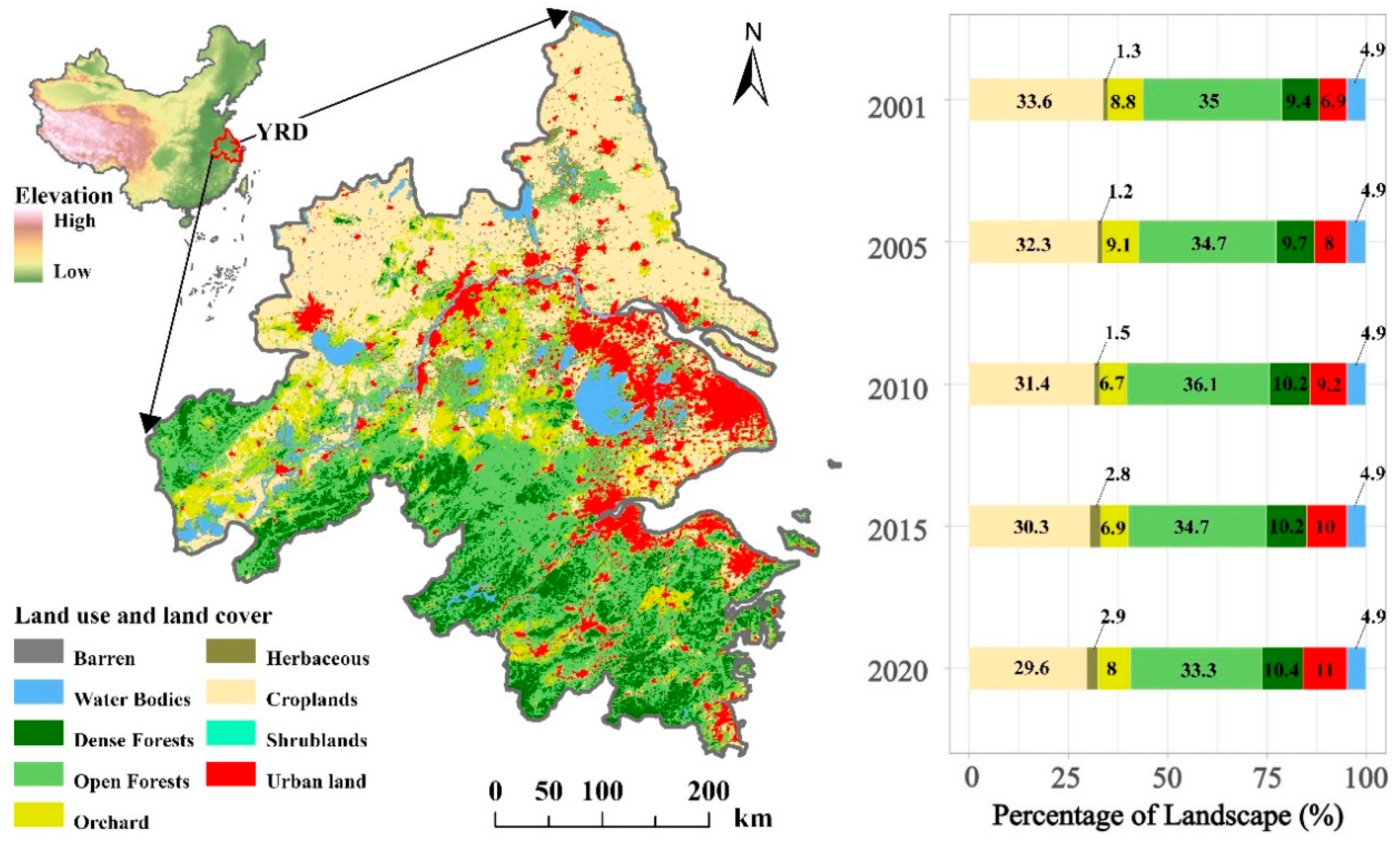
2.1. Study Area
2.2. Data Acquisition and Pre-Processing
2.3. Three Approaches for Calculating Ecosystem Service Trade-Offs and Synergies
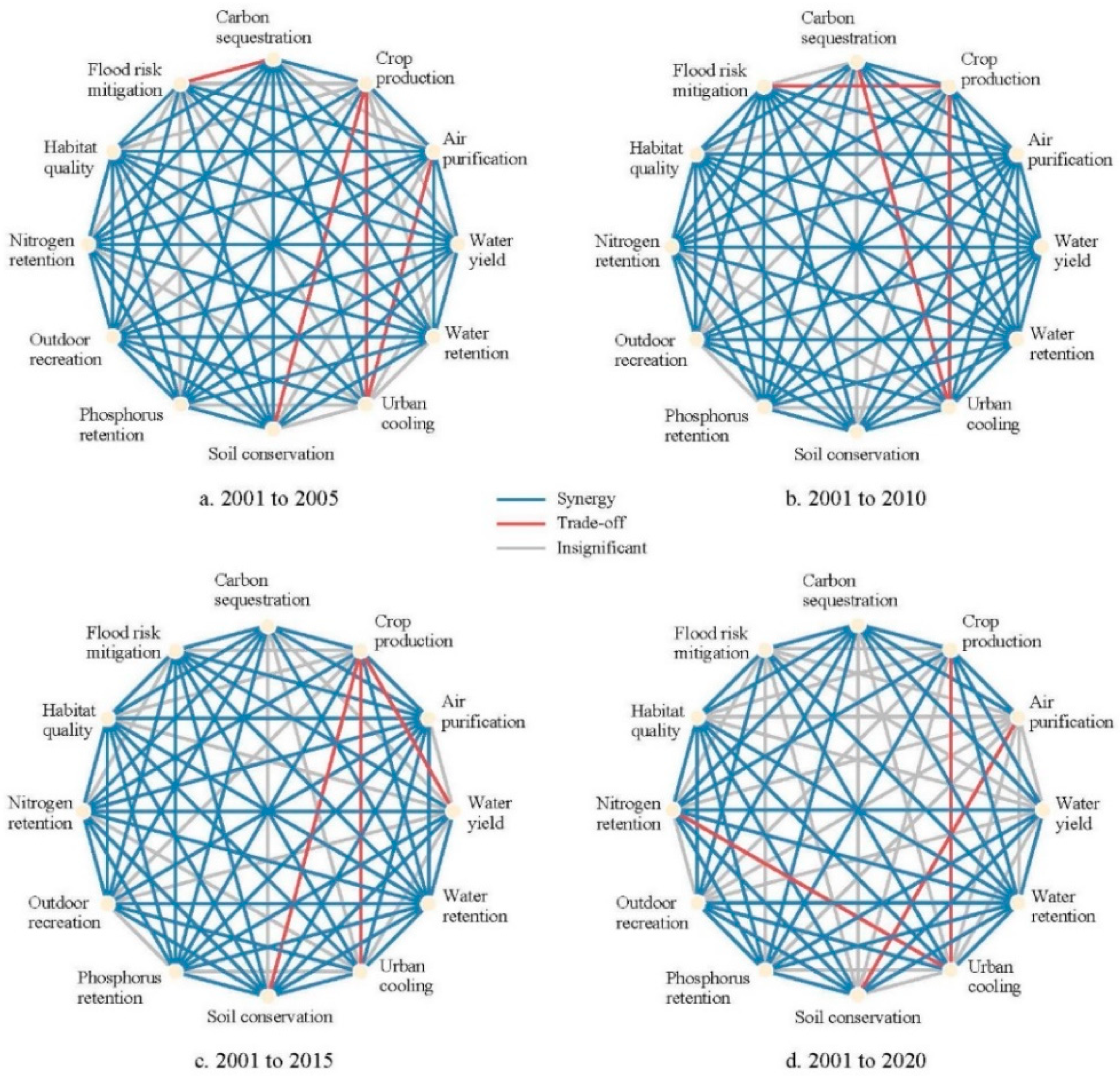
2.3.1. Space-for-Time Approach
2.3.2. Landscape Baseline-Adjusted Space-for-Time Approach
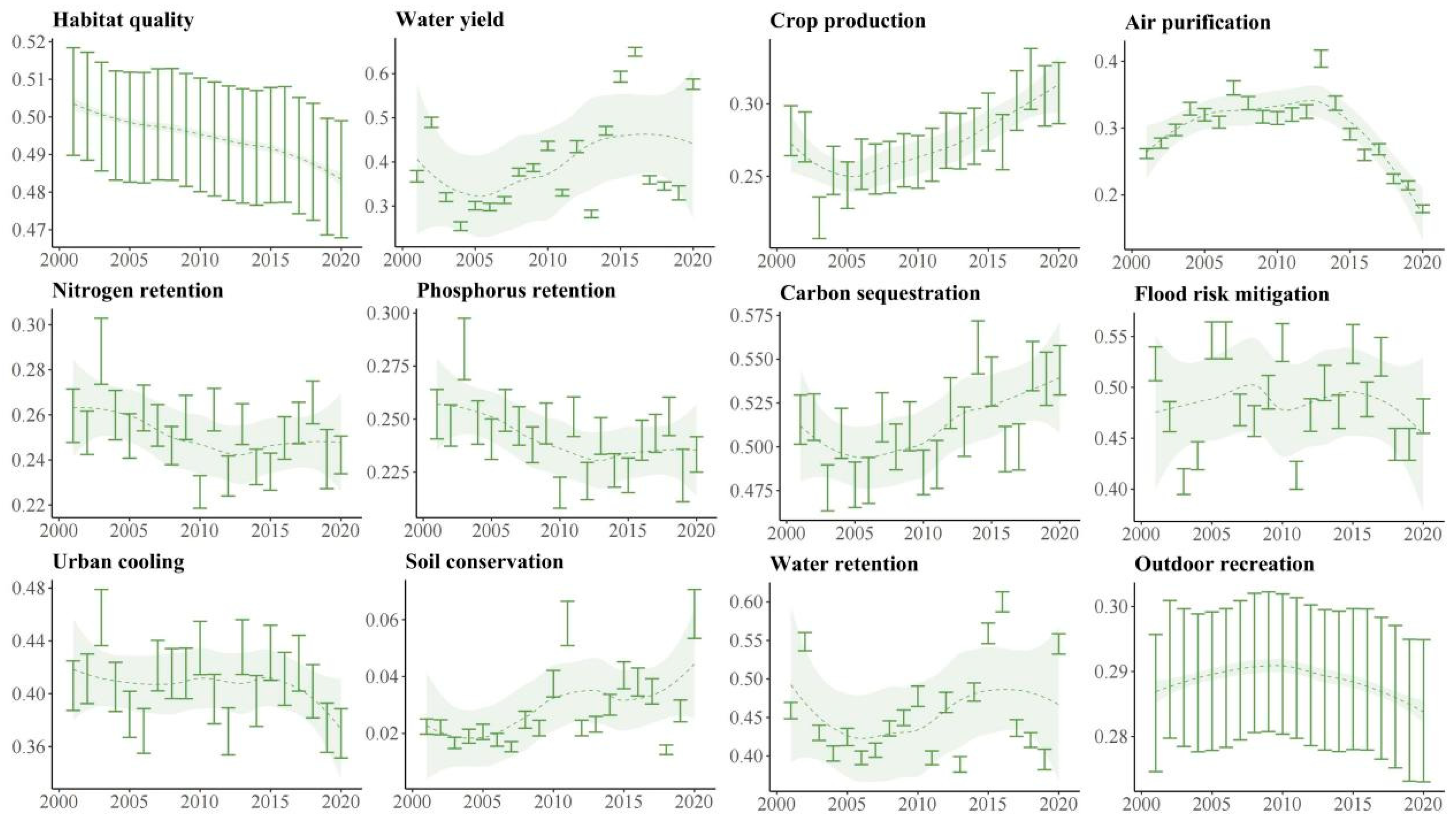
2.3.3. Temporal Trend Approach
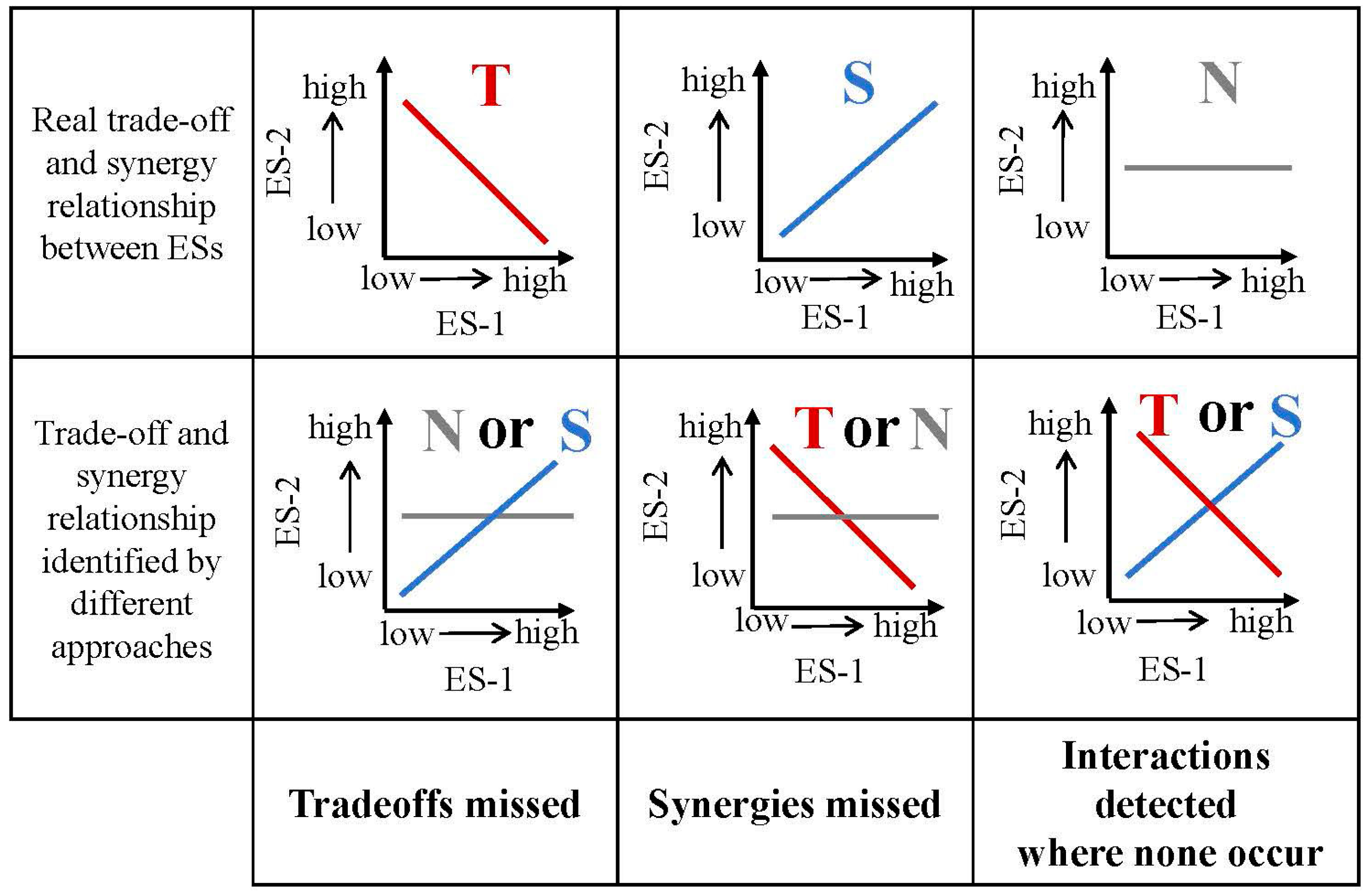
2.4. Three Possible Incorrect Ecosystem Service Relationships
3. Results
3.1. Space-for-Time Approaches in Different Time Frames
3.2. Landscape Baseline-Adjusted Space-for-Time Approach
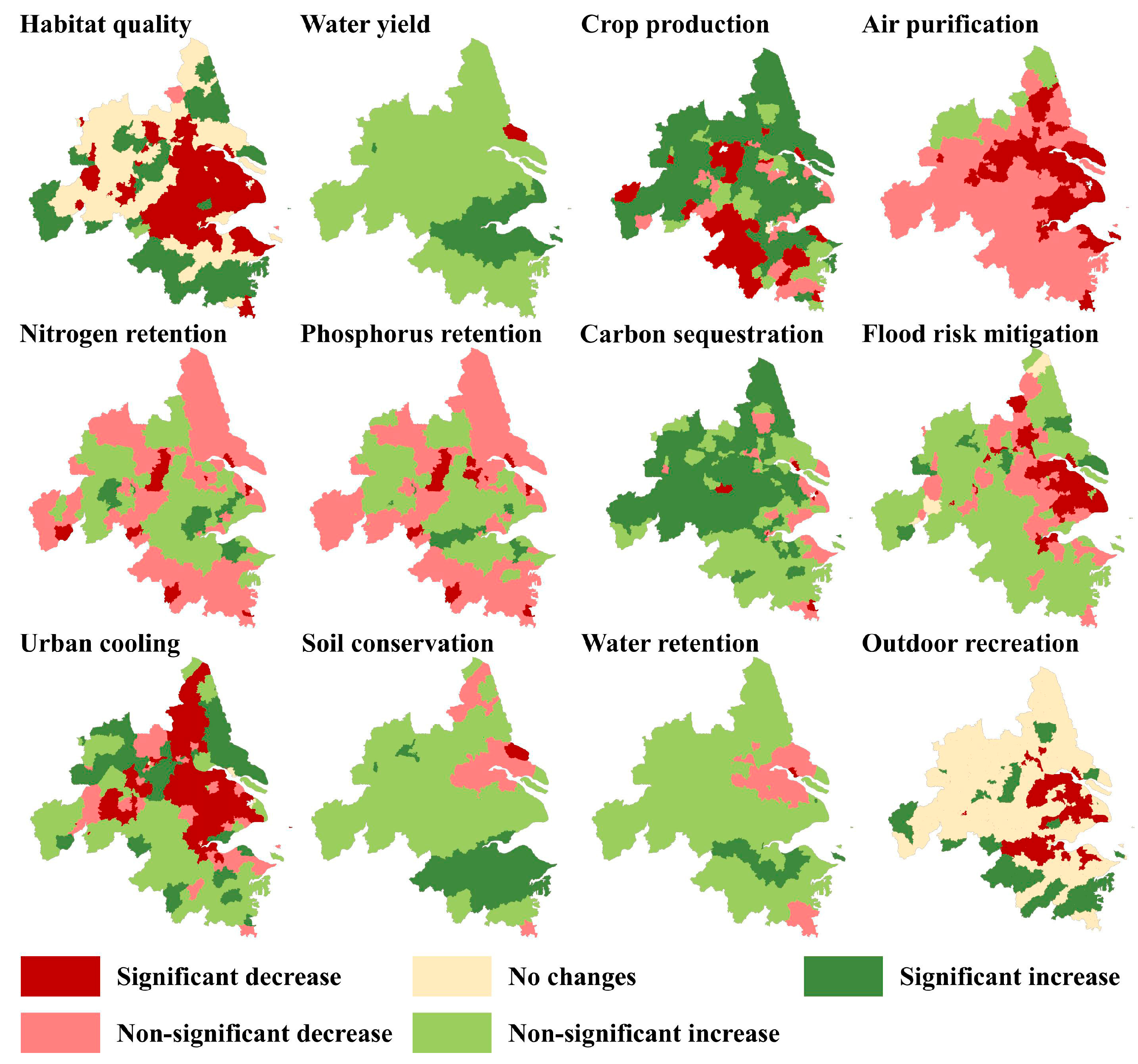
3.3. Temporal Trend Approach
4. Discussion
4.1. Little Disagreement Between Three Approaches
4.2. Mechanisms by Which the Three Approaches Produce Different ES Relationships
4.2.1. Ignoring the Assumptions of the SFT Method May Lead to the Identification of Incorrect ES Relationships
4.2.2. The Lack of Sufficiently Early Landscape Background ES Data Leads to the Misidentification of ES Relationships by the BA-SFT Method
4.2.3. The Time Span of Time Series Data, Data Aggregation Effects, and Time Lag Effects Lead to Errors in Identifying Relationships Between ES in the TT Method
4.3. Implications for Choosing Suitable Methods for Calculating ES Relationships
5. Conclusions
Supplementary Materials
Author Contributions
Funding
Data Availability Statement
Conflicts of Interest
References
- Wu, J. Landscape sustainability science: Ecosystem services and human well-being in changing landscapes. Landsc. Ecol. 2013, 28, 999–1023. [Google Scholar] [CrossRef]
- Fang, X.; Ma, Q.; Liu, Z.; Wu, J. Landscape sustainability and land sustainability: A bibliometric analysis. Land Use Policy 2024, 147, 107374. [Google Scholar] [CrossRef]
- Pereira, P.; Zhao, W. Geography and geographical knowledge contribute decisively to all sustainable development goals and targets. Geogr. Sustain. 2025, 6, 100267. [Google Scholar] [CrossRef]
- Dade, M.C.; Bonn, A.; Eigenbrod, F.; Felipe-Lucia, M.R.; Fisher, B.; Goldstein, B.; Holland, R.A.; Hopping, K.A.; Lavorel, S.; lede Polain Waroux, Y.; et al. Landscapes—A lens for assessing sustainability. Landsc. Ecol. 2025, 40, 28. [Google Scholar] [CrossRef]
- Qiu, J.; Nassauer, J.I.; Ahern, J.; Huang, L.; Reed, J.; Ding, S.; Guo, J.; Liu, Z.; Ou, W.; Ouyang, Z.; et al. Advancing landscape sustainability science: Key challenges and strategies for integration with landscape design and planning. Landsc. Ecol. 2025, 40, 1–10. [Google Scholar] [CrossRef]
- Fu, B.; Wu, X.; Wang, S.; Zhao, W. Scientific principles for accelerating the Sustainable Development Goals. Geogr. Sustain. 2024, 5, 157–159. [Google Scholar] [CrossRef]
- Rodríguez, J.P.; Beard, T.D., Jr.; Bennett, E.M.; Cumming, G.S. Trade-offs across Space, Time, and Ecosystem Services. Ecol. Soc. 2005, 11, 709–723. [Google Scholar] [CrossRef]
- Chan, K.M.; Shaw, M.R.; Cameron, D.R.; Underwood, E.C.; Daily, G.C. Conservation planning for ecosystem services. PLoS Biol. 2006, 4, e379. [Google Scholar] [CrossRef]
- Tallis, H.; Kareiva, P.; Marvier, M.; Chang, A. An ecosystem services framework to support both practical conservation and economic development. Proc. Natl. Acad. Sci. USA 2008, 105, 9457–9464. [Google Scholar] [CrossRef]
- Bennett, E.M.; Peterson, G.D.; Gordon, L.J. Understanding relationships among multiple ecosystem services. Ecol. Lett. 2009, 12, 1394–1404. [Google Scholar] [CrossRef]
- Raudsepp-Hearne, C.; Peterson, G.D.; Bennett, E.M. Ecosystem service bundles for analyzing tradeoffs in diverse landscapes. Proc. Natl. Acad. Sci. USA 2010, 107, 5242–5247. [Google Scholar] [CrossRef] [PubMed]
- Qiu, J.; Turner, M.G. Spatial interactions among ecosystem services in an urbanizing agricultural watershed. Proc. Natl. Acad. Sci. USA 2013, 110, 12149–12154. [Google Scholar] [CrossRef] [PubMed]
- Tomscha, S.A.; Gergel, S.E. Ecosystem service trade-offs and synergies misunderstood without landscape history. Ecol. Soc. 2016, 21, 43. [Google Scholar] [CrossRef]
- Xia, H.; Yuan, S.; Prishchepov, A.V. Spatial-temporal heterogeneity of ecosystem service interactions and their social-ecological drivers: Implications for spatial planning and management. Resour. Conserv. Recycl. 2023, 189, 106767. [Google Scholar] [CrossRef]
- Liu, L.; Wu, J. Space cannot substitute for time in the study of the ecosystem services-human wellbeing relationship. Geogr. Sustain. 2025, 6, 100221. [Google Scholar] [CrossRef]
- Cao, Y.; Cao, Y.; Li, G.; Tian, Y.; Fang, X.; Li, Y.; Tan, Y. Linking ecosystem services trade-offs, bundles and hotspot identification with cropland management in the coastal Hangzhou Bay area of China. Land Use Policy 2020, 97, 104689. [Google Scholar] [CrossRef]
- Pereira, P.; Inácio, M.; Pinto, L.; Kalinauskas, M.; Bogdzevic, K.; Zhao, W. Mapping ecosystem services in urban and peri-urban areas. A systematic review. Geogr. Sustain. 2024, 5, 491–509. [Google Scholar] [CrossRef]
- Pickett, S.T. Space-for-time substitution as an alternative to long-term studies. In Long-Term Studies in Ecology: Approaches and Alternatives; Springer: Berlin/Heidelberg, Germany, 1989; pp. 110–135. [Google Scholar]
- Haase, D.; Schwarz, N.; Strohbach, M.; Kroll, F.; Seppelt, R. Synergies, Trade-offs, and Losses of Ecosystem Services in Urban Regions: An Integrated Multiscale Framework Applied to the Leipzig-Halle Region, Germany. Ecol. Soc. 2012, 17, 22. [Google Scholar] [CrossRef]
- Renard, D.; Rhemtulla, J.M.; Bennett, E.M. Historical dynamics in ecosystem service bundles. Proc. Natl. Acad. Sci. USA 2015, 112, 13411–13416. [Google Scholar] [CrossRef]
- Qiu, J.; Carpenter, S.R.; Booth, E.G.; Motew, M.; Zipper, S.C.; Kucharik, C.J.; Loheide Ii, S.P.; Turner, M.G. Understanding relationships among ecosystem services across spatial scales and over time. Environ. Res. Lett. 2018, 13, 054020. [Google Scholar] [CrossRef]
- Bürgi, M.; Silbernagel, J.; Wu, J.; Kienast, F. Linking ecosystem services with landscape history. Landsc. Ecol. 2014, 30, 11–20. [Google Scholar] [CrossRef]
- Shifaw, E.; Sha, J.; Li, X.; Bao, Z.; Ji, J.; Ji, Z.; Kassaye, A.Y.; Lai, S.; Yang, Y. Ecosystem services dynamics and their influencing factors: Synergies/tradeoffs interactions and implications, the case of upper Blue Nile basin, Ethiopia. Sci. Total Environ. 2024, 938, 173524. [Google Scholar] [CrossRef] [PubMed]
- Hu, B.; Kang, F.; Han, H.; Cheng, X.; Li, Z. Exploring drivers of ecosystem services variation from a geospatial perspective: Insights from China’s Shanxi Province. Ecol. Indic. 2021, 131, 108188. [Google Scholar] [CrossRef]
- Wang, J.; Zhou, W.; Guan, Y. Optimization of management by analyzing ecosystem service value variations in different watersheds in the Three-River Headwaters Basin. J. Environ. Manag. 2022, 321, 115956. [Google Scholar] [CrossRef]
- Liu, X.; Li, L.; Qin, F.; Li, Y.; Chen, J.; Fang, X. Ecological policies enhanced ecosystem services in the Hunshandak sandy land of China. Ecol. Indic. 2022, 144, 109450. [Google Scholar] [CrossRef]
- Zhong, Z.; Fang, X.; Li, J.; Ma, Q.; Zhou, R.; Hu, Y.; Du, S. Linear and non-linear dynamics of ecosystem services supply, demand, and mismatches across a rapidly urbanizing region. Ecol. Indic. 2024, 158, 111614. [Google Scholar] [CrossRef]
- Zhang, Z.; Liu, Y.; Wang, Y.; Liu, Y.; Zhang, Y.; Zhang, Y. What factors affect the synergy and tradeoff between ecosystem services, and how, from a geospatial perspective? J. Clean. Prod. 2020, 257, 120454. [Google Scholar] [CrossRef]
- Deng, X.; Li, Z.; Gibson, J. A review on trade-off analysis of ecosystem services for sustainable land-use management. J. Geogr. Sci. 2016, 26, 953–968. [Google Scholar] [CrossRef]
- Sun, X.; Ye, D.; Shan, R.; Peng, Q.; Zhao, Z.; Sun, J. Effect of physical geographic and socioeconomic processes on interactions among ecosystem services based on machine learning. J. Clean. Prod. 2022, 359, 131976. [Google Scholar] [CrossRef]
- Li, X.; Deng, S.; Ma, X. Mechanism analysis of ecosystem services (ES) changes under the proposed supply-demand framework: A case study of Jiangsu Province, China. Ecol. Indic. 2022, 144, 109572. [Google Scholar] [CrossRef]
- Rova, S.; Meire, P.; Müller, F.; Simeoni, M.; Pranovi, F. A Petri net modeling approach to explore the temporal dynamics of the provision of multiple ecosystem services. Sci. Total Environ. 2019, 655, 1047–1061. [Google Scholar] [CrossRef] [PubMed]
- Fang, X.; Li, J.; Ma, Q.; Zhou, R.; Du, S. A quantitative review of nature-based solutions for urban sustainability (2016–2022): From science to implementation. Sci. Total Environ. 2024, 927, 172219. [Google Scholar] [CrossRef] [PubMed]
- Reid, W.V.; Mooney, H.A.; Cropper, A.; Capistrano, D.; Carpenter, S.R.; Chopra, K.; Dasgupta, P.; Dietz, T.; Duraiappah, A.K.; Hassan, R. Ecosystems and Human Well-Being-Synthesis: A Report of the Millennium Ecosystem Assessment; Island Press: Washington, DC, USA, 2005. [Google Scholar]
- Xu, X.; Yang, G.; Tan, Y.; Liu, J.; Hu, H. Ecosystem services trade-offs and determinants in China’s Yangtze River Economic Belt from 2000 to 2015. Sci. Total Environ. 2018, 634, 1601–1614. [Google Scholar] [CrossRef]
- Gao, J.; Yu, Z.; Wang, L.; Vejre, H. Suitability of regional development based on ecosystem service benefits and losses: A case study of the Yangtze River Delta urban agglomeration, China. Ecol. Indic. 2019, 107, 105579. [Google Scholar] [CrossRef]
- Liu, W.; Zhan, J.; Zhao, F.; Zhang, F.; Teng, Y.; Wang, C.; Chu, X.; Kumi, M.A. The tradeoffs between food supply and demand from the perspective of ecosystem service flows: A case study in the Pearl River Delta, China. J. Environ. Manage. 2022, 301, 113814. [Google Scholar] [CrossRef]
- Nowak, D.J.; Hirabayashi, S.; Bodine, A.; Hoehn, R. Modeled PM2.5 removal by trees in ten U.S. cities and associated health effects. Environ. Pollut. 2013, 178, 395–402. [Google Scholar] [CrossRef]
- Jiang, B.; Bai, Y.; Chen, J.; Alatalo, J.M.; Xu, X.; Liu, G.; Wang, Q. Land management to reconcile ecosystem services supply and demand mismatches—A case study in Shanghai municipality, China. Land Degrad. Dev. 2020, 31, 2684–2699. [Google Scholar] [CrossRef]
- Paracchini, M.L.; Zulian, G.; Kopperoinen, L.; Maes, J.; Schägner, J.P.; Termansen, M.; Zandersen, M.; Perez-Soba, M.; Scholefield, P.A.; Bidoglio, G. Mapping cultural ecosystem services: A framework to assess the potential for outdoor recreation across the EU. Ecol. Indic. 2014, 45, 371–385. [Google Scholar] [CrossRef]
- Chen, Y.; Liu, J. Derivation and generalization of the urban gravitational model using fractal idea with an application to the spatial cross-correlation between Beijing and Tianjin. Geogr. Res. 2002, 21, 742–752. [Google Scholar]
- Wei, Z.; Ren, Z.; Zhang, C. Analysis on the time-lag correlation between vegetation and climatic factors: Take Guangxi as an example. Ecol. Environ. Sci. 2013, 22, 1757–1762. [Google Scholar]
- Asadolahi, Z.; Salmanmahiny, A.; Sakieh, Y.; Mirkarimi, S.H.; Baral, H.; Azimi, M. Dynamic trade-off analysis of multiple ecosystem services under land use change scenarios: Towards putting ecosystem services into planning in Iran. Ecol. Complex. 2018, 36, 250–260. [Google Scholar] [CrossRef]
- Ouyang, Z.; Zheng, H.; Xiao, Y.; Polasky, S.; Liu, J.; Xu, W.; Wang, Q.; Zhang, L.; Xiao, Y.; Rao, E.; et al. Improvements in ecosystem services from investments in natural capital. Science 2016, 352, 1455–1459. [Google Scholar] [CrossRef] [PubMed]
- Tao, Y.; Tao, Q.; Sun, X.; Qiu, J.; Pueppke, S.G.; Ou, W.; Guo, J.; Qi, J. Mapping ecosystem service supply and demand dynamics under rapid urban expansion: A case study in the Yangtze River Delta of China. Ecosyst. Serv. 2022, 56, 101448. [Google Scholar] [CrossRef]
- Sun, X.; Li, F. Spatiotemporal assessment and trade-offs of multiple ecosystem services based on land use changes in Zengcheng, China. Sci. Total Environ. 2017, 609, 1569–1581. [Google Scholar] [CrossRef]
- Li, B.; Chen, N.; Wang, Y.; Wang, W. Spatio-temporal quantification of the trade-offs and synergies among ecosystem services based on grid-cells: A case study of Guanzhong Basin, NW China. Ecol. Indic. 2018, 94, 246–253. [Google Scholar] [CrossRef]
- De’Ath, G. Multivariate regression trees: A new technique for modeling species–environment relationships. Ecology 2002, 83, 1105–1117. [Google Scholar]
- Zuo, L.; Gao, J. Investigating the compounding effects of environmental factors on ecosystem services relationships for Ecological Conservation Red Line areas. Land Degrad. Dev. 2021, 32, 4609–4623. [Google Scholar] [CrossRef]
- Zheng, D.; Wang, Y.; Hao, S.; Xu, W.; Lv, L.; Yu, S. Spatial-temporal variation and tradeoffs/synergies analysis on multiple ecosystem services: A case study in the Three-River Headwaters region of China. Ecol. Indic. 2020, 116, 106494. [Google Scholar] [CrossRef]
- Sun, X.; Jiang, Z.; Liu, F.; Zhang, D. Monitoring spatio-temporal dynamics of habitat quality in Nansihu Lake basin, eastern China, from 1980 to 2015. Ecol. Indic. 2019, 102, 716–723. [Google Scholar] [CrossRef]
- Chen, D.; Jiang, P.; Li, M. Assessing potential ecosystem service dynamics driven by urbanization in the Yangtze River Economic Belt, China. J. Environ. Manag. 2021, 292, 112734. [Google Scholar] [CrossRef]
- Donohue, R.J.; Roderick, M.L.; McVicar, T.R. Roots, storms and soil pores: Incorporating key ecohydrological processes into Budyko’s hydrological model. J. Hydrol. 2012, 436, 35–50. [Google Scholar] [CrossRef]
- Budyko, M.I. Climate and Life; Academic Press: Cambridge, MA, USA, 1974. [Google Scholar]
- Allen, R.G.; Pereira, L.S.; Raes, D.; Smith, M.J.F. Crop evapotranspiration-Guidelines for computing crop water requirements-FAO Irrigation and drainage paper 56. FAO Irrig. Drain. Pap. 1998, 56, 29–64. [Google Scholar]
- González-García, A.; Palomo, I.; González, J.A.; López, C.A.; Montes, C. Quantifying spatial supply-demand mismatches in ecosystem services provides insights for land-use planning. Land Use Policy 2020, 94, 104493. [Google Scholar] [CrossRef]
- Zhou, R.; Lin, M.; Gong, J.; Wu, Z. Spatiotemporal heterogeneity and influencing mechanism of ecosystem services in the Pearl River Delta from the perspective of LUCC. J. Geogr. Sci. 2019, 29, 831–845. [Google Scholar] [CrossRef]
- Wischmeier, W.H.; Smith, D.D. Predicting Rainfall Erosion Losses: A Guide to Conservation Planning; Department of Agriculture, Science and Education Administration: Washington, DC, USA, 1978.
- Zawadzka, J.; Harris, J.A.; Corstanje, R.J.L.; Planning, U. Assessment of heat mitigation capacity of urban greenspaces with the use of InVEST urban cooling model, verified with day-time land surface temperature data. Landsc. Urban Plan. 2021, 214, 104163. [Google Scholar] [CrossRef]
- Stewart, I.D.; Oke, T.R. Local climate zones for urban temperature studies. Bull. Am. Meteorol. Soc. 2012, 93, 1879–1900. [Google Scholar] [CrossRef]
- Taha, H.; Akbari, H.; Rosenfeld, A.; Huang, J. Residential cooling loads and the urban heat island—The effects of albedo. Build. Environ. 1988, 23, 271–283. [Google Scholar] [CrossRef]
- NRCS, USDA. Estimation of direct runoff from storm rainfall. In National Engineering HandbookÀPart; NRCS, USDA: Washington, DC, USA, 2004; p. 630. [Google Scholar]
- Zhong, Z.; Fang, X.; Zhang, Y.; Shu, X.; Guo, D. Mapping Ecosystem Service Supply–Demand Bundles for an Integrated Analysis of Tradeoffs in an Urban Agglomeration of China. Land 2022, 11, 1558. [Google Scholar] [CrossRef]
- Jiang, H.; Peng, J.; Dong, J.; Zhang, Z.; Xu, Z.; Meersmans, J. Linking ecological background and demand to identify ecological security patterns across the Guangdong-Hong Kong-Macao Greater Bay Area in China. Landsc. Ecol. 2021, 36, 2135–2150. [Google Scholar] [CrossRef]
- Hamel, P.; Guerry, A.D.; Polasky, S.; Han, B.; Douglass, J.A.; Hamann, M.; Janke, B.; Kuiper, J.J.; Levrel, H.; Liu, H.; et al. Mapping the benefits of nature in cities with the InVEST software. Npj Urban Sustain. 2021, 1, 25. [Google Scholar] [CrossRef]
- Wu, Y.; Tao, Y.; Yang, G.; Ou, W.; Pueppke, S.; Sun, X.; Chen, G.; Tao, Q. Impact of land use change on multiple ecosystem services in the rapidly urbanizing Kunshan City of China: Past trajectories and future projections. Land Use Policy 2019, 85, 419–427. [Google Scholar] [CrossRef]
- Zhao, J.; Li, C. Investigating Ecosystem Service Trade-Offs/Synergies and Their Influencing Factors in the Yangtze River Delta Region, China. Land 2022, 11, 106. [Google Scholar] [CrossRef]
- Natural Capital Project. InVEST 3.12.0.post26+ug.g230fb3d User’s Guide; Stanford University, University of Minnesota, Chinese Academy of Sciences, The Nature Conservancy, World Wildlife Fund, and Stockholm Resilience Centre. 2022. Available online: https://storage.googleapis.com/releases.naturalcapitalproject.org/invest-userguide/latest/index.html (accessed on 15 March 2025).
- Villamagna, A.M.; Angermeier, P.L.; Bennett, E.M. Capacity, pressure, demand, and flow: A conceptual framework for analyzing ecosystem service provision and delivery. Ecol. Complex. 2013, 15, 114–121. [Google Scholar] [CrossRef]
- Licheng, L.; Chunfang, L.; Chuan, W.; Pengjie, L.I. Supply and demand matching of ecosystem services in loess hilly region: A case study of Lanzhou. Prog. Chem. 2019, 74, 1921. [Google Scholar]


| Ecosystem Service Types | Description | Quantification Methods |
|---|---|---|
| The ability of ecosystems to provide organisms with resources for survival and reproduction | InVEST |
| Capacity of farmland to produce crop | [37] |
| Capacity of ecosystems to provide freshwater | InVEST |
| Capacity of ecosystems to reduce the urban heat island effect | Urban InVEST |
| Capacity of urban ecosystems to reduce urban flood risk | Urban InVEST |
| Reduction in soil erosion due to the presence of vegetation | InVEST |
| Available water retained by ecosystems | InVEST |
| Amount of airborne pollutants absorbed by ecosystems. | [38] |
| Amount of nitrogen pollutants prevented from entering runoff by ecosystems | InVEST |
| Amount of phosphorus pollutants prevented from entering runoff by ecosystems | InVEST |
| Amount of carbon dioxide fixed by ecosystems | [39] |
| Opportunities for outdoor activities provided by ecosystems | [40] |
| Ecosystem Service Types | SFT & BA-SFT (%) | SFT & TT (%) | BA-SFT & TT (%) | Three Approaches (%) |
|---|---|---|---|---|
| Air purification | 33.33 | 25.00 | 75.00 | 16.67 |
| Crop production | 66.67 | 41.67 | 41.67 | 33.33 |
| Carbon sequestration | 58.33 | 16.67 | 33.33 | 16.67 |
| Flood risk mitigation | 58.33 | 16.67 | 58.33 | 16.67 |
| Habitat quality | 66.67 | 33.33 | 41.67 | 33.33 |
| Nitrogen retention | 41.67 | 16.67 | 41.67 | 16.67 |
| Outdoor recreation | 66.67 | 8.33 | 33.33 | 8.33 |
| Phosphorus retention | 41.67 | 25.00 | 41.67 | 25.00 |
| Soil conservation | 33.33 | 25.00 | 50.00 | 16.67 |
| Urban cooling | 58.33 | 16.67 | 58.33 | 16.67 |
| Water retention | 58.33 | 33.33 | 41.67 | 25.00 |
| Water yield | 33.33 | 8.33 | 50.00 | 8.33 |
| All | 46.97 | 15.15 | 42.42 | 1.45 |
Disclaimer/Publisher’s Note: The statements, opinions and data contained in all publications are solely those of the individual author(s) and contributor(s) and not of MDPI and/or the editor(s). MDPI and/or the editor(s) disclaim responsibility for any injury to people or property resulting from any ideas, methods, instructions or products referred to in the content. |
© 2025 by the authors. Licensee MDPI, Basel, Switzerland. This article is an open access article distributed under the terms and conditions of the Creative Commons Attribution (CC BY) license (https://creativecommons.org/licenses/by/4.0/).
Share and Cite
Zhong, Z.; Zhou, B.; Kong, L.; Fang, X. When to Use What: A Comparison of Three Approaches to Quantify Relationships Among Ecosystem Services. Land 2025, 14, 644. https://doi.org/10.3390/land14030644
Zhong Z, Zhou B, Kong L, Fang X. When to Use What: A Comparison of Three Approaches to Quantify Relationships Among Ecosystem Services. Land. 2025; 14(3):644. https://doi.org/10.3390/land14030644
Chicago/Turabian StyleZhong, Zhen, Bochuan Zhou, Lingqiang Kong, and Xuening Fang. 2025. "When to Use What: A Comparison of Three Approaches to Quantify Relationships Among Ecosystem Services" Land 14, no. 3: 644. https://doi.org/10.3390/land14030644
APA StyleZhong, Z., Zhou, B., Kong, L., & Fang, X. (2025). When to Use What: A Comparison of Three Approaches to Quantify Relationships Among Ecosystem Services. Land, 14(3), 644. https://doi.org/10.3390/land14030644