Article

autoRA: An Algorithm to Automatically Delineate Reference Areas—A Case Study to Map Soil Classes in Bahia, Brazil

by
Hugo Rodrigues
1,*,
Marcos Bacis Ceddia
1,2,
Gustavo Mattos Vasques
3,
Sabine Grunwald
4,
Ebrahim Babaeian
5 and
André Luis Oliveira Villela
6
1
Laboratory of Soil and Water in Agroecosystems (LASA), Postgraduation in Soil Science, Agronomy Institute, Federal Rural University of Rio de Janeiro, Seropédica 23890-000, Brazil
2
Agrotechnology and Sustainability Department, Agronomy Institute, Federal Rural University of Rio de Janeiro, Seropédica 23890-000, Brazil
3
Brazilian Research Brazilian Agricultural Research Corporation—Soils, Rio de Janeiro 22460-000, Brazil
4
Pedometrics, Landscape Analysis & GIS Laboratory, Soil, Water, and Ecosystem Sciences Department, University of Florida, Gainesville, FL 32611, USA
5
Environmental Soil Physics Lab, Soil, Water, and Ecosystem Sciences Department, University of Florida, Gainesville, FL 32611, USA
6
Technical College of the Federal Rural University of Rio de Janeiro, Rio de Janeiro 23897-000, Brazil
*
Author to whom correspondence should be addressed.
Land 2025, 14(3), 604; https://doi.org/10.3390/land14030604
Submission received: 8 February 2025 / Revised: 1 March 2025 / Accepted: 11 March 2025 / Published: 13 March 2025
(This article belongs to the Special Issue Predictive Soil Mapping Contributing to Sustainable Soil Management)

Abstract

:
The reference area (RA) approach has been frequently used in soil surveying and mapping projects, since it allows for reduced costs. However, a crucial point in using this approach is the choice or delineation of an RA, which can compromise the accuracy of prediction models. In this study, an innovative algorithm that delineates RA (autoRA—automatic reference areas) is presented, and its efficiency is evaluated in Sátiro Dias, Bahia, Brazil. autoRA integrates multiple environmental covariates (e.g., geomorphology, geology, digital elevation models, temperature, precipitation, etc.) using the Gower’s Dissimilarity Index to capture landscape variability more comprehensively. One hundred and two soil profiles were collected under a specialist’s manual delineation to establish baseline mapping soil taxonomy. We tested autoRA coverages ranging from 10% to 50%, comparing them to RA manual delineation and a conventional “Total Area” (TA) approach. Environmental heterogeneity was insufficiently sampled at lower coverages (autoRA at 10–20%), resulting in poor classification accuracy (0.11–0.14). In contrast, larger coverages significantly improved performance: 30% yielded an accuracy of 0.85, while 40% and 50% reached 0.96. Notably, 40% struck the best balance between high accuracy (kappa = 0.65) and minimal redundancy, outperforming RA manual delineation (accuracy = 0.75) and closely matching the best TA outcomes. These findings underscore the advantage of applying an automated, diversity-driven strategy like autoRA before field campaigns, ensuring the representative sampling of critical environmental gradients to improve DSM workflows.

1. Introduction

Soil sampling is essential for characterizing soil classes and properties in environmental, agronomic, and natural resource studies [1,2,3,4,5]. One common way to structure soil sampling is to define a reference area (RA), which are small subregions that capture the variability of soil-forming factors and represent larger areas [6,7,8,9]. Traditionally, experts manually delineate RAs using their knowledge and covariate maps such as land use, geomorphology, and climate to establish boundaries encompassing the variability of soil properties within the broader area of interest [9,10,11]. While this approach leverages professional experience, it can suffer from limited reproducibility, objectivity, and scalability [8,12]. These challenges stem from difficulty applying an expert’s mental model and synthesizing complex environmental information in highly variable areas, potentially compromising the RA methodology.
Despite the promise of RA methodologies in optimizing soil sampling, they face significant limitations due to the lack of automated techniques for identifying the most variable areas. Studies have demonstrated various challenges, such as those of Lagacherie et al. [13]. who highlighted the difficulty in ensuring that small RAs accurately represent more significant regions using mathematical soilscape distances, which may not always be reliable. Arruda et al. [8] achieved an accuracy of 82% using artificial neural networks with RAs, but the approach remains preliminary and may not capture the complexity of larger areas. Lagacherie et al. [13,14] and Yigini and Panagos [15] encountered issues in accurately predicting soil properties and ensuring data transferability from RAs to broader regions. Additionally, Gonçalves et al. [16] reported only moderate accuracy when extrapolating soil maps from small to large areas, indicating that current RA methods may struggle with scalability and representativity. While RA approaches provide a structured framework for soil mapping, the absence of automated methods to identify and delineate the most variable areas limits their effectiveness and scalability in large, environmentally complex regions.
The total area (TA) approach, widely used in digital soil mapping (DSM) workflows, treats the entire study region as a single dataset [17,18,19,20,21,22]. This method requires that soil sampling covers the whole area, which can be resource-intensive and time-consuming, especially for large and complex regions. The dataset is typically divided randomly into training and validation subsets, commonly using a 70/30 split. To validate the trained models, various statistical methods are employed, including cross-validation, which repeatedly trains and tests the model on different data subsets; k-fold cross-validation, which partitions the data into k folds and iteratively trains on k−1 folds while validating on the remaining fold; and out-of-the-bag (OOB) validation, often used with ensemble methods like random forests, which utilizes bootstrap samples for training and the unused samples for validation. These validation techniques are applied across multiple iterations, and the results are aggregated to assess model reproducibility and classification performance [23].
In pursuit of more systematic methods, researchers in Pedometrics and DSM have developed advanced sampling schemes that leverage modern computational and sensor technologies [24,25,26,27]. Conditioned Latin hypercube sampling (cLHS), for example, statistically balances soil covariates by partitioning the covariate space to ensure all quartiles of key soil-forming factors are represented [28,29]. However, cLHS does not rely on the RA hypothesis and instead depends on the TA approach, requiring comprehensive sampling across the entire study region. To enhance cLHS’s practicality, Malone et al. [29] addressed challenges such as optimizing sample size, relocating inaccessible sites, and prioritizing under-sampled areas by providing customized R scripts, making cLHS more adaptable to real-world field conditions. Additionally, Saurette et al. [30] introduced divergence metrics like Kullback–Leibler and Jensen–Shannon divergences to determine optimal training sample sizes, improving the methodological framework for DSM by ensuring more accurate and efficient sample designs.
Despite these advancements, both cLHS and the methodologies proposed by Saurette et al. remain grounded in the TA approach, as they do not incorporate the RA framework. In this study, we hypothesize that an automated method for delineating RA significantly reduces subjectivity and makes the approach more effective (better accuracy of prediction models and lower cost for soil mapping). This automation enhances reproducibility and scalability, facilitating the broader adoption of RA-based methods within the Pedometrics community.
We introduce autoRA (automatic reference area), a novel algorithm that locates and delineates RA based on covariate maps commonly applied in DSM workflows using Gower’s Dissimilarity Index. Costa et al. [31] (in Pedometrics in Brazil) utilized this index to identify the most heterogeneous regions in Rio de Janeiro, highlighting that the covariate values were notably high, indicating significant regional differences. This high variability suggests that sampling soil from these heterogeneous areas can yield a diverse dataset, which is crucial for effective digital soil modeling. Their approach underscores the importance of selecting representative regions to enhance the accuracy and reliability of predictive models in soil science.
AutoRA allows the user to generate a new RA for an area without previous mapping (legacy data) and can also be used to evaluate whether a given RA, previously delimited conventionally (manually), could be better delineated (size and shape). In this study, we present autoRA to (i) assess how well soil class maps are generated via autoRA compared to those produced from a manually delineated RA and (ii) to evaluate both RA-based methods (manually and by autoRA) against the TA approach in terms of sampling efficiency, reproducibility, and classification accuracy.

2. Materials and Methods

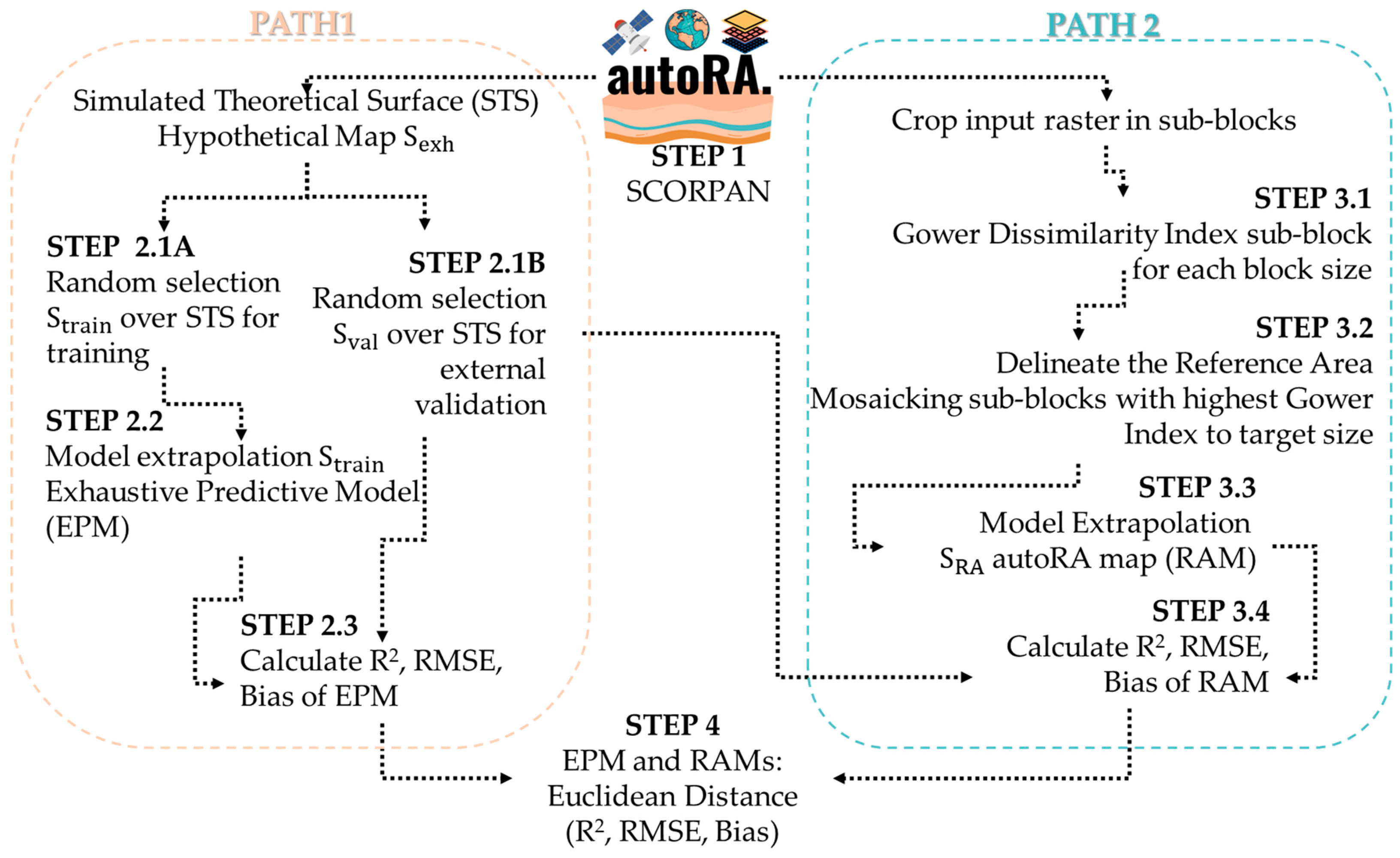
2.1. The autoRA Algorithm

Figure 1 summarizes the patented autoRA approach (BR1020240208676; trademark 937505684) for the automatic delineation of RAs in soil mapping, which is already registered in Brazil and will soon be registered at the United States Patent Office. In STEP 1, the user assembled the geospatial datasets { X 1 , X 2 , , X p } representing SCORPAN factors (soil, climate, organisms, relief, parent material, age, and spatial neighborhood) [32]. Each X j can be numeric (continuous/discrete) or categorical (nominal/ordinal). The original resolution of these covariates constrains the minimal block size that can later be used in RA delineation.
The workflow proceeded along Path 1 and Path 2 in parallel. Path 1 began with STEP 2.1A, where randomly sampled n training points { ( x i , y i , s i ) } from an “exhaustive” simulated soil surface (Sexh or STS) represent a hypothetical ground truth of the soil property of interest S e x h . Every pixel in the AOI had a known value s i , and this was used to build a random forest model [33] to predict S e x h from the covariates  f RF : X 1 , , X p s ^ e x h .
In STEP 2.1B, an independent validation set { ( x i , y i , s i ) } j = i m was also randomly sampled over the entire area of interest to assess model accuracy via the performance metrics R2 (Equation (1)), RMSE (Equation (2)), and bias (Equation (3)) for observed s j vs. predicted s ^ j .
R 2 = 1 j = 1 m ( s ^ j s j ) 2 j = 1 m ( s ¯ j s j ) 2
where s ¯ j = 1 m j = 1 m s j
R M S E = 1 m j = 1 m ( s ^ j s j ) 2
B i a s = 1 m j = 1 m ( s ^ j s j ) 2
STEP 2.2 applied f R F to the entire AOI’s covariate stacks to produce the “exhaustive” predictive surface S E P M , and STEP2.3 served as an ideal reference for subsequent performance comparisons. S E P M finalizes this “exhaustive” predictive model (EPM) as a ground truth benchmark.
Our study uses the term “Benchmark MU map” to denote a gold standard target map derived from extensive field data. We do not intend this term to be interpreted as a formal jargon or an extension of the well-established concept of Benchmark Soils. Instead, it is employed descriptively to identify the most reliable and representative mapping product against which alternative soil mapping approaches (e.g., RA manual is the benchmark and autoRA, and TA are comparisons) are evaluated. This clarification ensures that our focus remains on using the Benchmark MU map as a practical reference point for assessing mapping accuracy and methodological improvements, independent of the traditional Benchmark Soils framework [34].
It is important to note that the STS represents the gold standard or an exhaustive theoretical map reflecting one possible reality of the soilscape related to the interaction among the covariates used. However, in this study, since the original fieldwork and sampling design were based on the hypothesis of a reference area manually developed by a specialist, the STS created in autoRA Path 1 was replaced by the final soil map classes (RA manual) produced using the RA manual approach.
Path 2 represented the part of the algorithm that effectively created the RAs by cropping the input raster maps (RA by autoRA—Figure 1). It performed the autoRA sensitivity analysis to delineate RAs using two adjustable parameters—block size (5 to 150 pixels) and RA target area (10 to 50% of the AOI, in 10% increments).
In STEP 3.1, Gower’s Dissimilarity Index was computed per block for the SCORPAN covariates. For continuous covariates, a pair of blocks, i , j , represent the partial distance. X k is shown in Equation (4).
d k ( i , j ) = X k ( i ) X k ( j ) m a x X k ( i ) m i n X k ( i )
When dealing with categorical covariates, they were transformed to be dummy-based. For a nominal X l ,
d l ( i , j ) = 0 ,   i f   X l ( i ) = X l ( j ) 1 ,   otherwise
When dealing with ordinal variables, a rank was transformed into [0, 1] and treated as continuous. Finally, the combined Gower’s Dissimilarity for p covariates is given by Equation (5).
d G ( i , j ) = k = 1 p δ k ( i , j ) d k ( i , j ) k = 1 p δ k ( i , j )
where δ k ( i , j ) = 1 if both X k ( i ) and X k ( j ) are non-missing; otherwise, δ k ( i , j ) = 0 .
STEP 3.2 mosaiced the highest dissimilarity values above the mean, defining RA boundaries and generating multiple RAs of varying sizes. The block size parameter variation aggregated blocks of pixels in sizes from 5 to 150 pixels. The pixels with high dissimilarity were mosaicked, whose average d G concerned the AOI average if exceeding d ¯ G . These were merged to form candidate RAs. The final aggregation of high-dissimilarity pixels constrained the resulting RA to 10–50% of the total AOI (in increments of 10%) by adjusting thresholds on d G .
STEP 3.3 then sampled a fixed number of point samplings within each RA, drawing a fixed number of training points {( x r , y r )} to produce a new model fit for training a Reference Area Model (RAM) S ^ R A (using RF or another learner) in order to predict soil properties across the entire AOI while using just the RA sampled for training. The RAM validation process used an independent validation set to evaluate each RA’s predictive surface with the same metrics (R2, RMSE, and bias).
Finally, STEP 4 compared the RAM predictions from Path 2 to the EPM (from Path 1) using R2, RMSE, and bias. Euclidean Distance (ED) was calculated for each RA, as defined from a performance vector ( R R A 2 , R M S E R A , B i a s R A ) using Equation (6).
E D ( R A ) = ( R R A 2 1 ) 2 + R M S E R A 2 + B i a s R A 2
The RA that most minimized the ED (RA) was deemed the “best-performing”. The EPM from Path 1 serves as a benchmark to gauge how well each RA (Path 2) extrapolated to the entire AOI.
By coupling the STS benchmark with RA-based modeling, autoRA thus provided a robust way to test different RA dimensions and ensure accurate soil property predictions.

2.2. autoRA Heterogeneous Coverage and Extrapolation Formalization

Let Ω be the set of all possible spatial units (blocks or pixels) in an AOI. Each spatial unit x Ω was characterized by a feature vector X ( x ) R p , where p is the number of covariates, including both continuous and categorical covariates. Define the dissimilarity function d G [35] over Ω , and let D(Ω) be the maximum dissimilarity range found in the AOI, which is defined as the largest pairwise dissimilarity between any two spatial units in Ω, as given by Equation (7)
D Ω = max x , y Ω d G X x , X y
Equation (7) defines D(Ω) as the maximum dissimilarity, meaning the greatest observed distance between any two feature vectors in the AOI according to the Gower dissimilarity function. We aimed to find a subset Ω Ω , referred to as the RA, that “covers” a large portion of the AOI’s heterogeneity. Formally, we wanted
x Ω , r Ω such   that d G X x , X r δ ,
for some small δ > 0.
Suppose the AOI satisfied a Lipschitz-like condition [36] for a soil property  S , meaning that there existed a Lipschitz constant L > 0, such that [37]
S x S y L d G X x , X y , x , y Ω ,
for all spatial units x , y Ω , where   d G X x , X y was the dissimilarity between the feature vectors X x and X y and L > 0 was a constant that scaled the upper bound of the difference in S x .
In this way, small changes in the covariates led to proportionally small changes in S , with L controlling the sensitivity of S to variations in the covariate space. If Ω is an RA for which
m a x x , y Ω m i n r Ω d G X x , X r δ
a predictive model f trained on Ω can be extrapolated to Ω with the maximum error bounded by L δ [38]:
max x Ω S x f x L δ .
An RA Ω that captured the most heterogeneous pixels in the covariate space ensured good predictive coverage [39]. Under mild assumptions, if the RA encloses the full range of environmental variability, a soil model (e.g., using random forest algorithm) trained on Ω can be extrapolated to the remainder of the AOI, with limited error bounded by L δ . This underpins the autoRA rationale on which a small portion of the area is rich in heterogeneity, meaning that any unvisited point in the AOI remains “close” to some training point in Ω .

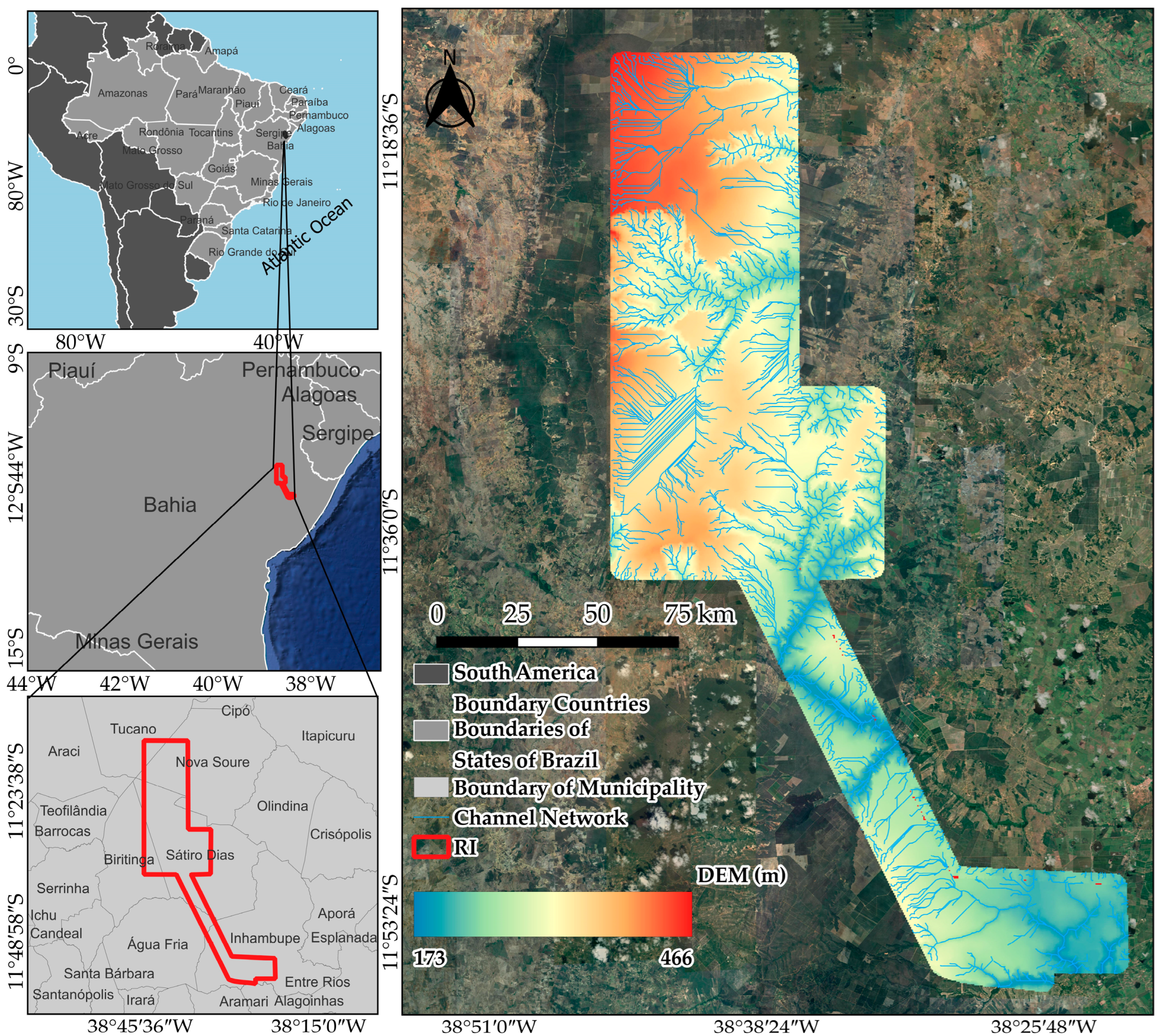
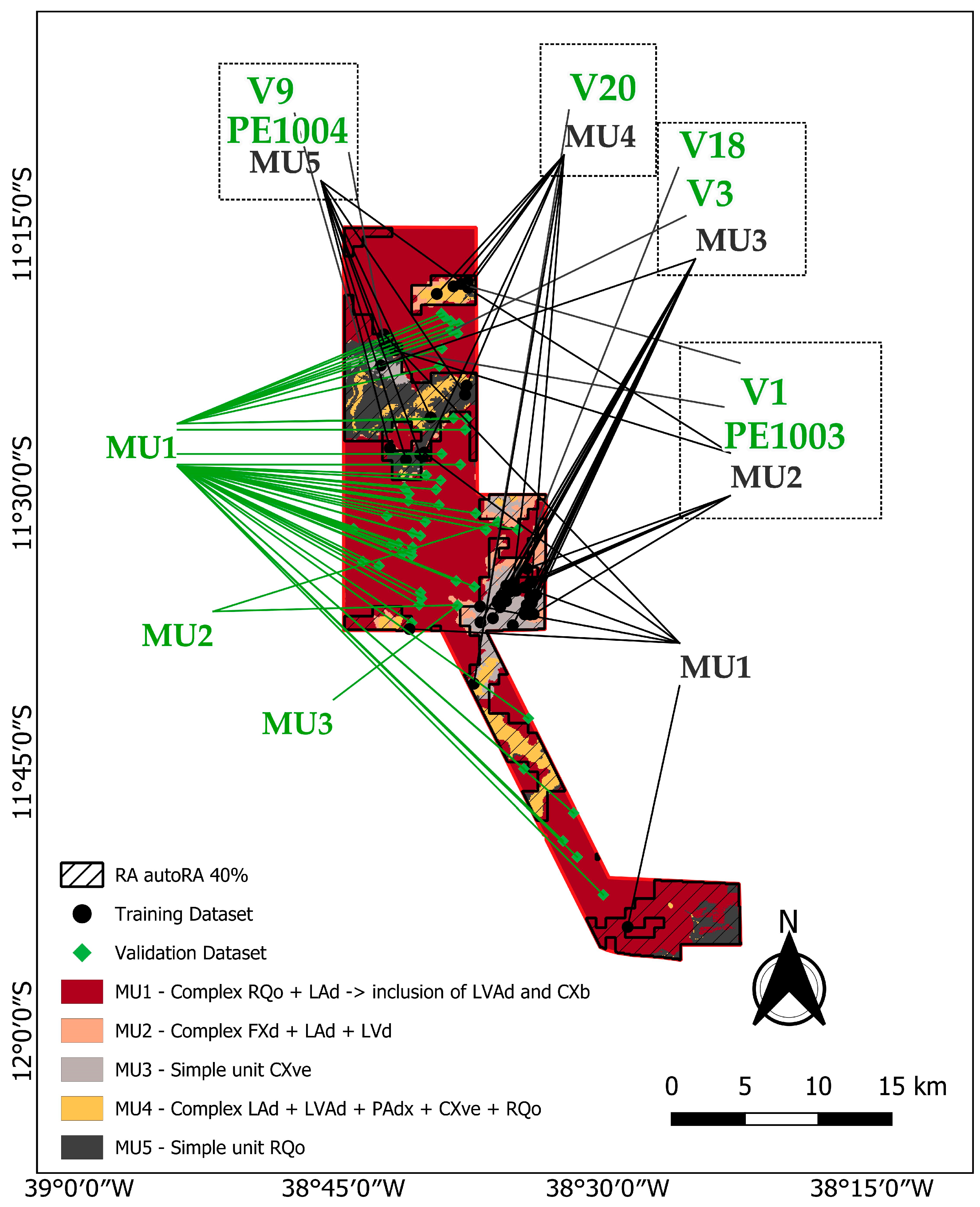
2.3. Study Area, Data Preparation, and Manual Delineation of Reference Area

The study was conducted in Sátiro Dias, Bahia, Brazil, covering a region of interest (RI) of 901 km2 (Figure 2). Before initiating fieldwork, the specialist compiled spatial co-variates influencing soil formation in the area. These covariates included geology, geomorphology, and pedology maps from the Brazilian Institute of Geography and Statistics (IBGE) at a 1:250,000 scale [40]. To enhance the environmental covariates for better comprehension, the specialist also considered the climatic data from WorldClim Version 2, representing monthly averages from 1970 to 2000, available at spatial resolutions ranging from 30 arc seconds (~1 km2) [41], including average annual precipitation and temperature maps. Additionally, the digital elevation model (DEM) from the Shuttle Radar Topography Mission provided by NASA was included [42], with a spatial resolution of 1 arc second (~30 m at the Equator). These data were critical for understanding the terrain-related factors influencing soil formation and representing the SCORPAN model [32]. The maps of the covariates used are presented in Figure 3.
The next step in delineating the RA manual is reviewing each covariate layer individually. The experts began by examining the covariate maps representing the key factors influencing soil formation (e.g., geology, geomorphology, climate, topography, vegetation). For each layer, the goal was to identify regions that collectively capture most of the variation or diversity in that layer. The cases with categorical layers identified polygons that include most (if not all) distinct classes (e.g., different geological units or geomorphology types). In a continuous layer, locating areas represented the full range of values (e.g., minimum to maximum elevations or precipitation). Once the experts pinpointed high-diversity regions for a specific layer, they delineated small polygons around these areas. These polygons effectively serve as “high-variation zones” for that layer—places where many classes or a broad range of values can be found in a relatively compact space.
After these diversity polygons were delineated for each covariate layer, they were overlaid and stacked in a GIS environment. This superposition allowed the experts to visualize where the diversity polygons from different layers intersected or overlapped, thereby revealing areas simultaneously representative of multiple factors (e.g., geology and topography). The experts drew a boundary encompassing all or most of the diverse polygons across layers to synthesize these overlapping polygons into a cohesive region. By doing so, they ensured that this final polygon—referred to as the “RA manual”—captured a broad spectrum of environmental conditions without becoming too large or unwieldy.
The RA manual was constrained to cover no more than 30% of the total region of interest (RI) to maintain feasibility for detailed soil investigations. Through iterative adjustments, the experts arrived at a final RA manual spanning approximately 212 km2 (Figure 3), striking a balance between capturing environmental heterogeneity and stabilizing the sampling area [43,44,45]. This approach was intended to ensure that the RA manual includes diverse environmental conditions while maintaining a manageable area for intensive soil.
Following the RA manual, the specialist applied the conditioned Latin hypercube algorithm [46] to allocate 74 sampling points within the RA manual using the environ-mental covariates listed. These points were used for the detailed observation and description of complete soil profiles, forming the primary dataset for model training. Additionally, 28 points were randomly distributed outside the RA manual to serve as an external validation dataset, ensuring the accuracy of models and maps constructed during the study (Figure 3).
The methodology comprised three main stages: (1) delineation of reference areas (RAs), (2) soil sampling simulation, and (3) soil classification modeling (Figure 4). Two approaches were used to delineate RAs: first, experts manually delineated an RA covering 212 km2 (RA manual), and second, the autoRA algorithm was employed to identify areas of maximum dissimilarity via Gower’s Dissimilarity Index (RA autoRA). By applying thresholds of 10%, 20%, 30%, 40%, and 50% of the highest dissimilarity values, multiple RA autoRA subsets were produced, each reflecting different levels of landscape variability.
In addition to these RA-based methods, a total area (TA) approach was implemented, treating the entire 901 km2 as a single dataset, randomly split into 70% for training and 30% for validation, repeated 100 times to minimize bias [47,48,49].
For the RA manual, 74 samples inside the boundary were used to train the soil classification model, and 28 samples outside were used for external validation (102 total). For each RA autoRA, boundaries were intersected with the aggregate (training + validation) soil sample dataset, defining samples within each RA as training points and those outside as external validation. In this way, only the autoRA Path 2 is applied to this research once there was no demand for a simulated theoretical surface.
The final soil classification stage involved creating three models: (1) RA manual-based models using the manually delineated RA samples, (2) RA autoRA-based models built from the various threshold-defined RA autoRA subsets, and (3) TA-based models using the entire dataset under the repeated 70/30 splits. Model performance was evaluated using overall accuracy and the kappa index, comparing manual and automated RA delineation alongside the aggregated TA approach, whose results were averaged over 100 iterations. An overview of the workflow applied in the present study is shown in Figure 4.
Table 1 presents the MU generated for the area of Sátiro Dias and their respective landscape characteristics. After correlating the soil types with the landscape attributes, five MUs were delineated as follows:
MU1—Plateau, flat to gently undulating relief: Soil complex composed of the main classes Quartzipsamment (RQo) and Dystrudept (CXvd), with a sandy loam texture and moderate A horizon, including Haplustox (LAd).
MU2—Upper and middle third of the plateau slopes: Soil complex composed of the main classes Petroplinthic Paleudult (FXd) and Petroplinthic Haplustox (LAd), with a sandy loam texture, moderate A horizon, and phase with epipedons, including Dystric Haplustox (LVd).
MU3—Region of hills at lower altitudes than plateaus (Sátiro Dias central region): Simple unit dominated by the class Typic Eutrudept (CXve), with a medium-clay texture and moderate A horizon, including occurrences of Argic Eutrudept (CXve), Paleudalf (LV), and Natric Haplotert (CXv) with moderate A horizons.
MU4—Region of hills within canyons: Soil complex composed of the classes Haplustox (LAd), Dystric Haplustox (LVAd), Petroplinthic Paleudult (PAdx), Typic Eutrudept (CXve), and Quartzipsamment (RQo).
MU5—Lowlands within canyons (North of Sátiro Dias): Simple unit occurrence of Quartzipsamment (RQo) with a very sandy texture and weak A horizon.
Figure 5 shows the map of soil classes (MU) in the region of Sátiro Dias. The MU1 (RQo + LAd + CXvd complex) is the one with the highest territorial expression (71%) since areas of sandy plateaus predominate. The MU with the second most significant territorial expression is MU3 (single unit CXve, 11%). This mapping unit is associated with hills at an altitude lower than the plateaus in the central region of Sátiro Dias. In this mapping unit, soils with clay of high activity and high base saturation (Ca++, Mg++, K+, and Na+) stand out.

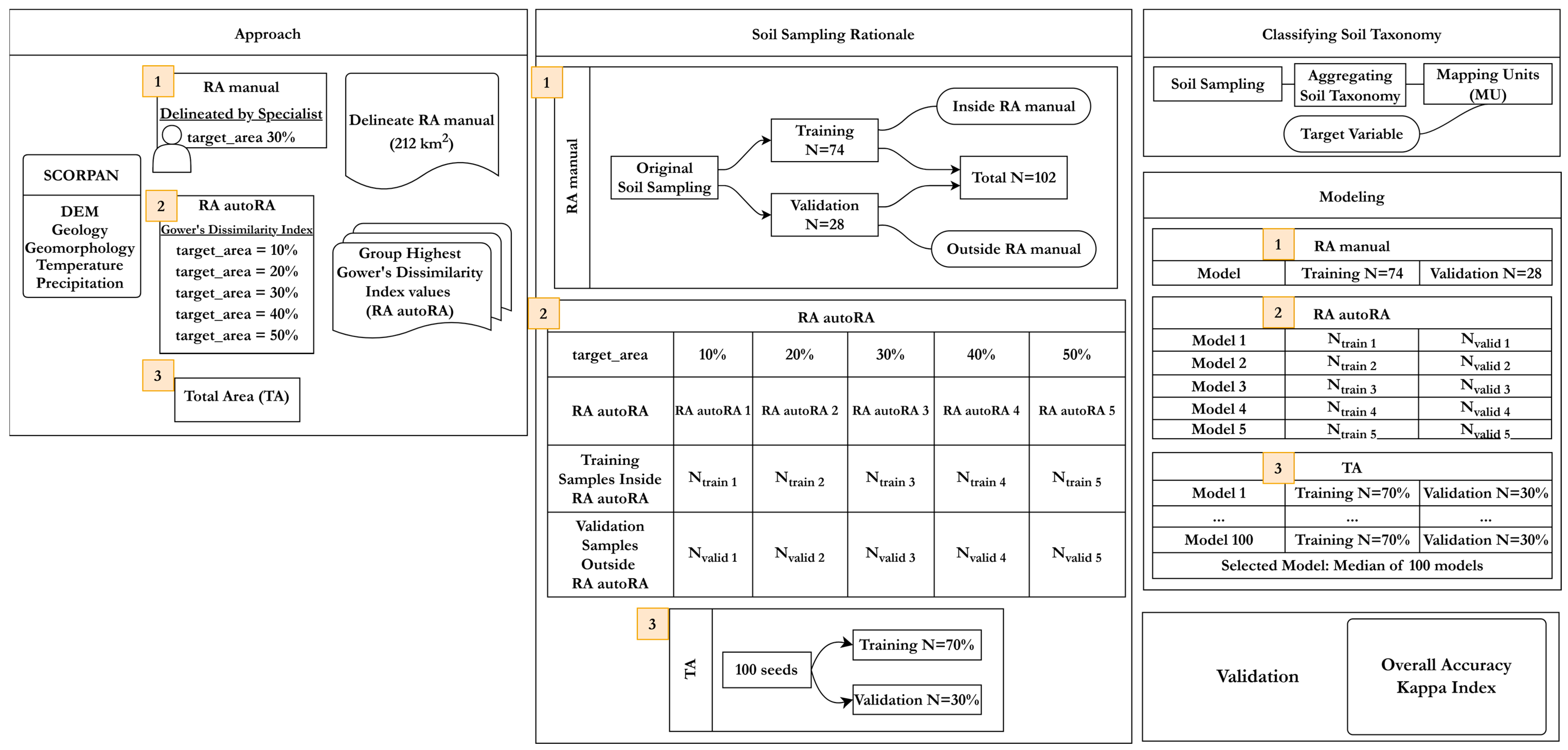
2.4. Soil Sampling Regrouping and Spatial Prediction Using the Reference Area and the Total Area Dataset

The original soil sampling dataset comprised 102 points, 74 designated for training and 28 for external validation, collected both within and outside the RA manual, respectively. These 102 soil profiles were used to simulate the dataset for the RA autoRA. To assess the efficacy of RA autoRA delineations, the sampling points were reassigned based on their spatial relation to each RA autoRA subset. Points intersected within the RA autoRA boundaries for each threshold (10%, 20%, etc.) were designated as part of the training set for that specific RA autoRA scenario. In contrast, points located outside the RA autoRA boundaries were reserved as the external validation set.
For all approaches tested (manual RA, RA autoRA, and total area—TA), the random forest (RF) algorithm was used to predict the five mapping units. The package random forest [33] present in the R software (Version 4.4.3) [50] was used. For the RA autoRA mapping procedure, the training dataset varied regarding the number of profiles. The number of training and validation profiles for each RA was a direct consequence of the intersection of the RA polygon generated by autoRA (10, 20, 30, 40, and 50%) with the profile points surveyed in the field (102). Thus, the profiles inside the reference RA polygon were used for training, while those outside were used to validate the prediction models. For the TA approach, the 102 soil samples were split into training and validation using the 70% and 30% ratio, respectively. To reduce the randomization effect during the sampling process, it was repeated 100 times, and, consequently, 100 RF were adjusted.
The RF’s fit parameters of the model were maintained by the default defined by the package’s authors, in which the number of trees was 500. The minimum amount of data in each terminal node parameter has been set to the default of five for each terminal node. Regarding the number of variables used in each tree, for classification problems, the default value is one-third of the total predictor variables.

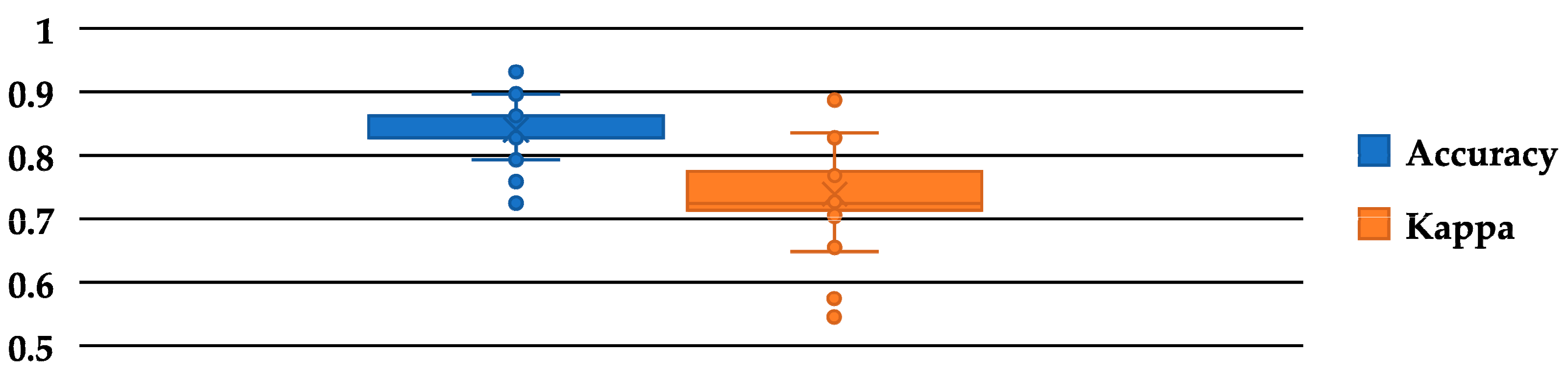
2.5. Accuracy of the Mapping Unit Maps

The following quality measures were used to assess the quality of the predicted MU maps: overall accuracy (OA), kappa coefficient of agreement, User’s Accuracy (UA), and Producer’s Accuracy (PA). All of them were based on the confusion matrix [3] and were calculated as the proportion of the samples or soil types correctly predicted over the total number of validation locations (reference field data). The OA was given by Equation (8) [3].
O A = i = 1 c E i j n
in which E is the confusion or error matrix of dimensions c × c and n is the number of samples (observations). In the literature, overall accuracy is also called overall purity, map purity, global accuracy, and general accuracy [3]. UA is given by Equation (9).
U A = E u E i u
in which E i u denotes the number of points mapped as the mapping unit u, that is, the sum of the rows in the confusion matrix, and E u are the classes correctly classified in unit u, the main diagonal of the confusion matrix. The complement of UA (1 − UA) is referred to as the error of commission (inclusion), that is, the error ruled by including pixels from other classes in the class in question. In the literature, other synonyms are also used for User’s Accuracy, such as map unit purity [3], which is about predicted classes (map) [51]. The PA is given by Equation (10).
P A = E u E j u
in which E j u denotes the number of points mapped as the mapping unit u, that is, the sum of the columns in the confusion matrix, and E u are the classes correctly classified in unit u, the main diagonal of the confusion matrix. The complement of PA (1 − PA) is referred to as the omission errors (exclusion) when a pixel ceases to be classified correctly in that mapping unit and is incorrectly classified as another unit. In the literature, other synonyms are also used for Producer’s Accuracy, such as class representation or ground truth (reference field data) [51]. The kappa index is given by Equation (11).
k ^ = n i = 1 c E i j i = 1 c E i E j n 2 i = 1 c E i E j
where c is the number of classes on the matrix, E i j represents the values on row i and column i , E i is the total on row i , E j is the total on column  j , and  n  is the number of samples (observations).
Finally, as different soil maps of the same study site using RA manual, RA autoRA, and TA approaches were compared, the indexes WPAI (Weighted Producer Accuracy Index) and WUAI (Weighted User Accuracy Index) were also computed (Equations (12) and (13), respectively).
Generating the WUAI and WPAI indices aimed to give a global view of each map’s user and producer accuracy. Thus, as in each map, the mapping units had different territorial expressions. Both indexes were weighted averages of user and producer accuracy. The weighting was performed by multiplying this OA by the area of each MU divided by the total area of the map (A).
The WUAI and WPAI indices allowed us to know how the types of errors are distributed (commission or omission, respectively) in each map (give an overview of these errors for a specific map). Thus, after comparing the OA and the kappa index, before entering into the detailed evaluation of the types of errors per mapping unit (which is conventionally carried out), we used the WUAI and WPAI indices to compare the relevance of commission and omission errors on each map (five generated by RA autoRA, one by TA, and one by RA manual generated by RF). The index values range from 0 to 1, with 0 lacking OA and 1 being the maximum OA.
W P A I = j n E u E j u * a u A
in which E j u denotes the number of points mapped as the mapping unit u , that is, the sum of the columns in the confusion matrix; E u represents the classes correctly classified in that unit u , the main diagonal of the confusion matrix; a u is the surface area of the mapped unit u ; and A is the total surface area of the map.
W U A I = i n E u E i u * a u A
in which E i u denotes the number of points mapped as the mapping unit u , that is, the sum of the rows in the confusion matrix; E u are the classes correctly classified in that unit u , the main diagonal of the confusion matrix; a u is the surface area of the mapped unit u ; and A is the total surface area of the map.

3. Results and Discussion

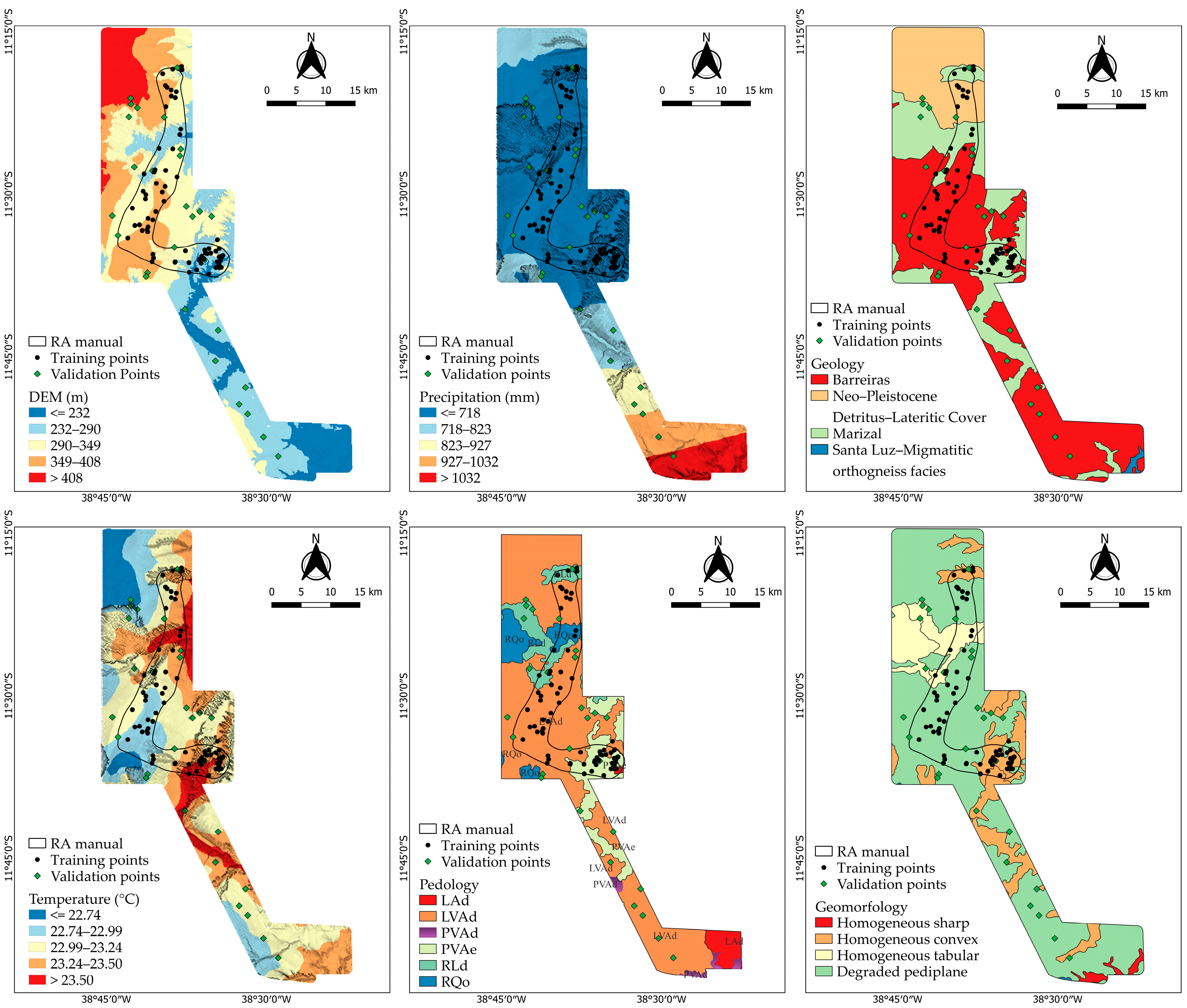
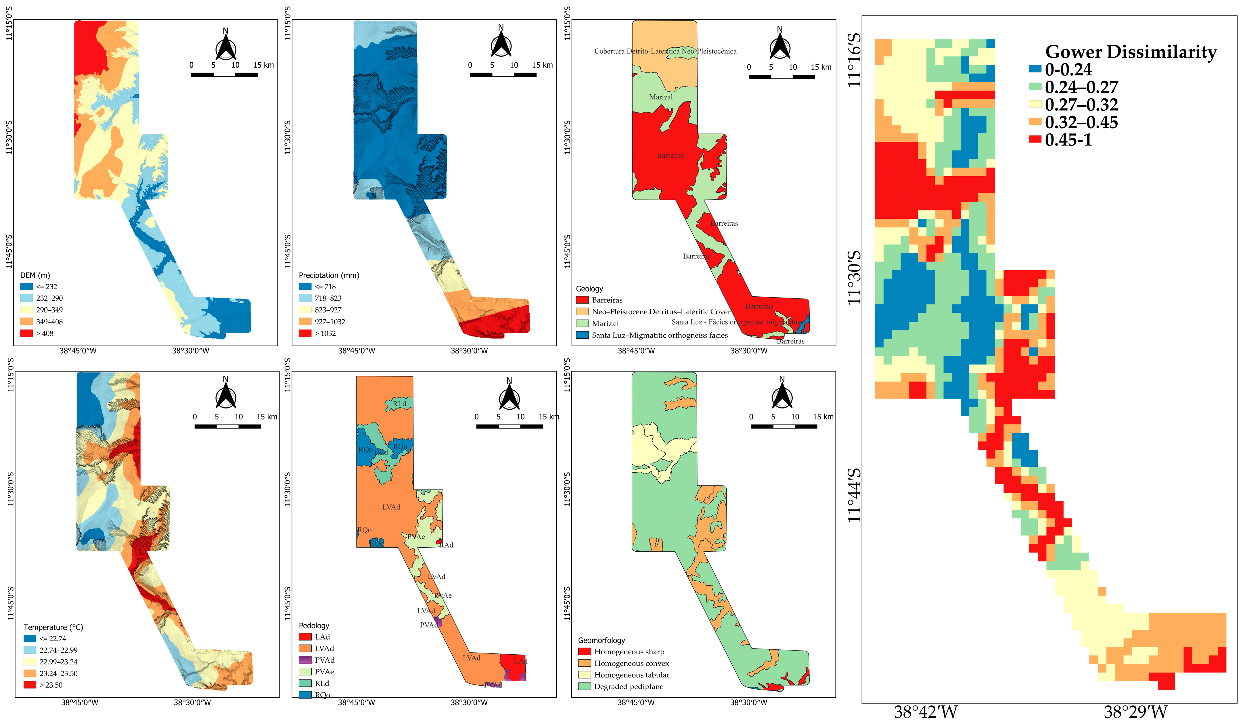
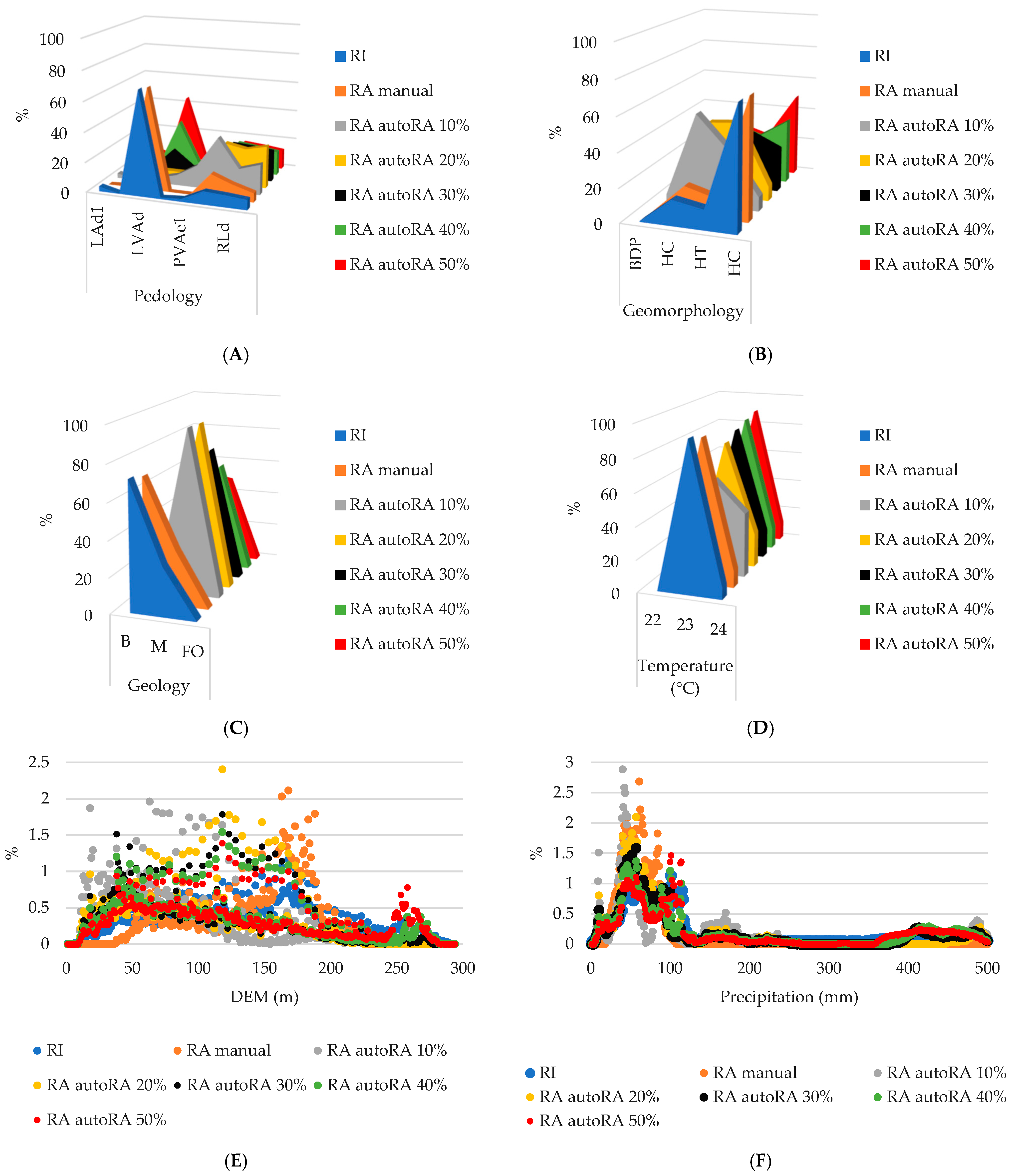
3.1. Soil Landscape Relationship and Spatial Distribution

The benchmark for this study was the MU map created during the original field campaign project, which serves as a reference for detailing the manually delineated reference areas (RA manual) and associated soil profiles. It is important to clarify that our use of the “Benchmark MU map” is intended to designate the target or reference map representing the highest achievable quality in our study, rather than introducing a new technical term derived from the concept of Benchmark Soils [34].
To provide an in-depth understanding, the study area has been divided into seven sections (Sections 1 through 7), each highlighting key soil profiles and their characteristics. These sections included detailed photos and descriptions of important profiles to illustrate the spatial variability and transitions within the region.
The first subregion (Section 1), as illustrated in Figure 6, covered the northern part of the RI, encompassing profiles PE006, PE007, and PE1008. Profile PE006, situated in an elevated and well-drained area, has sandy textures, whereas PE1008, located in flatter terrain, shows organic matter accumulation in the upper layers due to reduced drainage [52]. These differences align with the variability in geological and pedological covariates, emphasizing the critical influence of parent material and topography on soil properties in the region.
Additionally, profiles PE0006, PE0007, and PE1008 were representative soil types of transition characteristics between canyon and plateau regions in Nova Soure (Neighbor Municipality of Sátiro Dias). These profiles exhibited a medium-to-high degree of development on gently-to-strongly undulating slopes, occupying the middle and upper thirds of the landscape. A notable feature in this geological context (Marizal formation) is the frequent presence of surface gravel, ranging from slightly gravel to extremely gravel. In the subsurface, the soils display yellowish, reddish-yellow, and/or yellowish-red hues, resembling plateau soils but differing in the absence of surface gravel and exhibiting deeper, more developed profiles.
PE0006 may show mottling in the C horizons, linked to parent material fragments, reflecting the soil–rock interface’s transitional nature [53,54]. In the lower part of this region, sandy, deep, and sharply drained soils such as PE1008 are found (Figure 6). Despite its darker color, the soil was very sandy and had relatively homogeneous horizons between them. The horizons of these soils had a weak aggregation or even simple grain and a predominantly loose dry and wet consistency, in addition to not having plasticity and stickiness.
Figure 7 represents Section 2, which features soil profiles PE1003 and PE1004 and the external validation point V2. Situated on a typical plateau, V2 represented the characteristic soil of upland regions, shaped by higher elevations and distinct geomorphological features. These soils are generally deep, well drained, and exhibit minimal surface stoniness, indicative of stable environmental conditions [20].
In contrast, PE1004 is located in a flat lowland area and is characterized by sandy, weathered, drained soils with a lighter color and no rocky material. The covariates, such as precipitation and geology, highlighted the influence of hydrological and geomorphic processes in these lowland terrains [55]. PE1003 occupies a transitional zone between the plateau and lowland regions. While it shares some characteristics with plateau soils, its moderate elevation and geomorphological transitions give it unique soil attributes that are reflective of its intermediary position.
Section 3, depicted in Figure 8, highlights the central portion of the region of interest (RI), focusing on profiles P806, PE808, and PE1007. Similarly to the patterns observed in the northern area (Figure 5), this central region distinguishes between lowland and plateau soils.
Profile P806 represents the lowland soils characterized by sandy, deep, and excessively drained conditions with minimal aggregation. In contrast, plateau soils, exemplified by profile PE808, occur in flat terrains free of stones and rocks. These soils are deep, well developed, and well drained, with sandy textures and subsurface colors ranging from brown to light brown, reflecting stable geomorphic conditions [56,57].
A notable feature in this section was the presence of mottling in profile PE1007, similar to that observed in PE006. This characteristic is attributed to the influence of the soil’s parent material and distinguishes it from the upper-third transitions and topsoil layers, where mottling is absent.
Section 4, representing the southern part of the RI, was illustrated in Figure 9 and features profiles P826, P834, and P853, demonstrating notable geological and geomorphological variability. Profile P853, situated on rocky substrata, has shallow horizons influenced by lithic contact, while P826 exhibits deeper profiles with significant clay accumulation in the subsurface. These variations align with earlier pedology maps, underscoring the critical role of geological features in driving soil variability and emphasizing the importance of accounting for geomorphological heterogeneity in soil classification and management strategies [58].
The central portion of Section 4 focuses on plateau soils near the municipalities of Sátiro Dias and Biritinga. These soils, derived predominantly from Marizal formation geological material, are deep, well drained, and well developed. They occur in non-stony, non-rocky terrain under native forest cover and in texture from sandy to medium. Subsurface colors exhibit a range from 5 YR to 7.5 YR hues, including yellow-brown, brown-yellow, brown, red-yellow, and reddish-brown tones, reflecting subtle but meaningful diversity in soil development processes.
Texturally, sandy loam dominates, but clay–silty loam and clayey loam were also present, highlighting the region’s complexity and variation. This diversity, shaped by the interaction of parent material, geomorphological setting, and vegetation cover, illustrates the area’s nuanced soil–landscape relationships.
Section 5, summarized in Figure 10, focused on the southeastern corner of the RI and highlighted profiles V11, V12, and PE003. This region captures significant climatic and geomorphological transitions, as reflected in the covariate data. Profiles V11 and V12 demonstrate distinct drainage characteristics shaped by local topography, while pedology and geology maps reveal variations in soil-forming processes, emphasizing the critical role of integrating topographic and climatic data for precise soil delineation [59].
In the eastern plateau region (Figure 10), profiles generally follow the patterns described for plateau soils. Profile V11 is characterized by a brown color and a loam-to-silty loam texture, while PE003 displays a red hue with a clay–silty loam texture. Both profiles are deep, well developed, and sharply drained, with minimal horizon differentiation and no surface stoniness. The redder coloration of PE003, compared to P868, likely reflects differences in parent material. This profile is located at the transition zone from the plateau, resembling PE1003, to an area where two canyons begin to diverge.
Profile V12, situated in a transition zone between the plateau and the canyon, is located on the upper third of a slope with undulating relief. The soil in this position is stony, well drained, and shallower than similar transitions observed in the northern region. Unlike northern counterparts, the soils here are more influenced by erosive and clayey processes, suggesting variability in source material despite the underlying geology associated with the Marizal formation [60]. Additionally, the soil exhibits mottling due to its parent material, with a brownish-yellow background color indicative of its transitional nature.
Section 6, illustrated in Figure 11, represents the western part of the region of interest (RI), highlighting profiles P875, P888, and V19. Profile P875 is characterized by reddish soils rich in iron oxides, reflecting its formation from specific geological materials, while profile P888 displays lighter horizons which are indicative of pronounced leaching and lower mineral content. These profiles underscore the influence of geological and climatic covariates on soil mineralogy, offering valuable insights for refined soil classification and management strategies [61].
In the southwestern region of Sátiro Dias, profiles from the extreme south of Section 6, such as V19, share similarities with previously described plateau soils. These profiles are typically brown with sandy loam textures, exhibiting characteristics consistent with stable geomorphic conditions under native forest cover. In contrast, profiles P875 and P888 have loam textures with distinct red-yellow and reddish-brown hues, respectively, reflecting variability in parent material and soil-forming processes.
The soils in this section are predominantly well-to-excessively drained, with textures ranging from loam to sandy loam. They are characterized by aggregates of weak development and small-to-minimal size, transitioning from granular structures at the surface to subangular blocks in the subsurface. A notable feature of plateau soils in this region is the presence of shallow horizons with a low degree of development, often classified as weakly developed or, at best, moderately developed diagnostic surface horizons [62]. This variability highlights the interaction of parent material, drainage, and geomorphic processes in shaping soil characteristics across the region.
Section 7, illustrated in Figure 12, highlights the southwestern corner of the region of interest (RI) and features profiles P868, PE005, and PE1006. Profile P868 is notable for its sharp transitions between horizons, indicative of high variability in soil-forming factors. At the same time, PE005 and PE1006 exemplify the influence of geomorphological patterns and precipitation gradients on soil development.
Profiles PE005 and PE1006 showcase significant differences despite their proximity. PE005 is characterized by a reddish color with dark red mottling, influenced by rock fragments rich in ferromagnesian minerals [63]. This young soil, situated on the upper third of a hill with undulating relief, exhibits abundant stoniness and a clay–silty loam texture with a high content of primary minerals, reflecting its less-developed state and strong lithological influence.
In contrast, PE1006, located in a flatter landscape nearby, represents a deep, well-developed soil with uniform horizons. Unlike PE005, it lacks stoniness or rockiness and aligns with the typical characteristics of plateau soils, illustrating the pronounced impact of landscape position on soil properties. These profiles highlight the intricate interplay between geomorphology, parent material, and drainage in shaping soil variability within this region.

3.2. The Gower Dissimilarity Index Map

The Gower Dissimilarity Index is a multivariate measure accommodating continuous and categorical variables. It is particularly suited for comparing diverse SCORPAN covariates (e.g., climate, topography, geology) in digital soil mapping. In Figure 13, the Gower Dissimilarity Index values are grouped into five classes (≤0.24 in blue, 0.24–0.27 in green, 0.27–0.32 in yellow, 0.32–0.45 in orange, and >0.45 in red), offering a spatially explicit overview of how similar or dissimilar different areas of the RI are in terms of their underlying environmental attributes.
Lower Gower Dissimilarity Index values (blue/green) highlight more uniform regions where soil and landscape characteristics remain relatively consistent—commonly aligned with dominant classes such as Typic Udults or Tabular Homogeneous. In contrast, the highest dissimilarities (red) mark zones of pronounced variability, often associated with transitions between markedly different geological or pedological settings, as seen in areas where Lithic Entisols and Eutrophic Udults with smooth relief converge or where “Tabular Homogeneous” meets “Degraded Pediplane”. The intermediate ranges (yellow/orange) capture subtle shifts or gradients, such as the southern part of the map where geology changes from “Barreiras” to “Santa Luz”.
Beyond indicating regions of high or low environmental uniformity, the Gower Dissimilarity Index map also aligns with variations in DEM and precipitation (notably higher in the northwest and lower in the south). By integrating multiple covariates into a single measure, the Gower Dissimilarity Index reveals the distinct soil-forming environments and the transitional zones that may warrant closer investigation or targeted sampling in future studies [64].

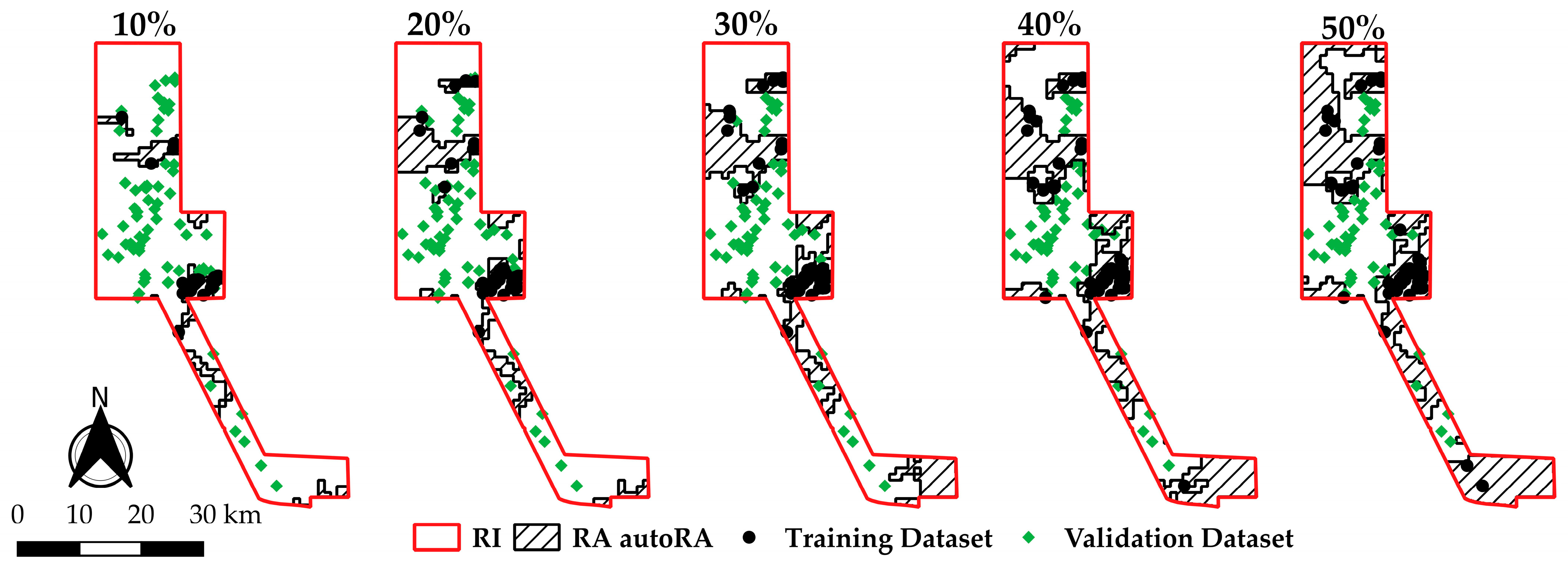
3.3. Reference Area Delineation Using autoRA and Associated Training and Validation Datasets

Figure 14 shows the spatial distribution of the training and validation datasets within the RA autoRA at varying target area percentages of the RI (10%, 20%, 30%, 40%, and 50%). The validation datasets (green points in Figure 14) remain distributed outside the autoRA-defined RA, serving as an external validation dataset to evaluate the performance of models constructed using the training data within each RA autoRA delineation.
At 10% coverage, the autoRA delineation captures 22 training points within the RA autoRA 10%, primarily focusing on areas with the highest Gower’s Dissimilarity Index values. The remaining 80 points fell outside the RA autoRA 10%, serving as validation data. As the RA autoRA expands to 20% and 30%, the number of training points increases to 38 and 43, respectively, while the validation points decrease correspondingly. This trend continues with larger RA autoRA target area sizes, reaching 51 training points and 51 validation points at 40% coverage and 53 training points and 49 validation points at 50% coverage. The manually delineated RA manual includes 74 training points within its boundaries, leaving 28 points for validation.
Figure 14 highlights the autoRA methodology’s capacity to adapt the RA boundaries to different levels of coverage while preserving the representativeness of soil-forming factors. Including points within regions with high Gower’s Dissimilarity Index values in smaller RA autoRA target area sizes demonstrates the algorithm’s focus on maximizing variability. Conversely, larger RAs enable a broader representation of the RI, which may benefit applications requiring wide spatial coverage.
Figure 15 compares the pixel distributions of the study’s covariates—pedology, geomorphology, geology, temperature, DEM, and precipitation—using RI (employed by the TA to capture overall area variability), manual RA, and autoRA at reduction levels of 10%, 20%, 30%, 40%, and 50%. The results indicate that as the reference area increases, autoRA effectively captures diverse patterns while reducing the Gower dissimilarity value. This aligns with McBratney’s concept in the Homosoils framework [9], where defining the optimal Gower Index cutoff is crucial for balancing representation and variability.
AutoRA at 30–40% closely matches RIs across all covariates. In pedology, LVAd and PVAd each represent ~35–40%, similar to RI’s ~40%, whereas manual RA over-represents LAd1 (~40%) and under-represents LVAd and PVAd (~25–30%). For geomorphology, autoRA at 30–50% balances BDP (~60–70%), HC (~30%), and HT (~10–15%) in alignment with RI, while manual RA over-represents HC (~35%) and under-represents BDP (~50%).
In geology, autoRA at 30–40% mirrors RI with category B (~40%), FO (~25%), and M (~35%), compared to manual RA, which over-represents category B (~70%) and under-represents FO (~10%) and M (~20%). Temperature is accurately captured by autoRA at 30–50%, maintaining the dominant 23 °C range (~60%) and adjacent transitions at 22 °C (~20–25%) and 24 °C (~15–20%), unlike manual RA, which under-represents the 23 °C range (~40%) and fails to capture adjacent temperatures.
For DEM, autoRA at 30–50% balances elevations across peaks (~250–300 m) and lower areas (~0–200 m), closely mirroring RI, whereas manual RA smooths the distribution and under-represents higher elevations. In precipitation, autoRA at 30–40% closely matches RI by distributing low (~2–3%), moderate (~1.5–2%), and high (~0.5%) precipitation ranges. At the same time, manual RA oversimplifies the distribution, over-representing low precipitation (~4%) and under-representing moderate (~1%) and high (<0.5%) ranges.
To further substantiate these findings, the Gower Index cutoff values for each % of RA (10, 20, 30, 40, and 50%) highlight how autoRA objectively determines the optimal balance between variability and representativeness. Lower autoRA thresholds (10–20%) significantly diverge from RI, whereas autoRA at 30–40% minimizes dissimilarity while maintaining diversity. A 50% reduction introduces minor over-representations in some variables, such as lower elevations in DEM and LAd1 in pedology.

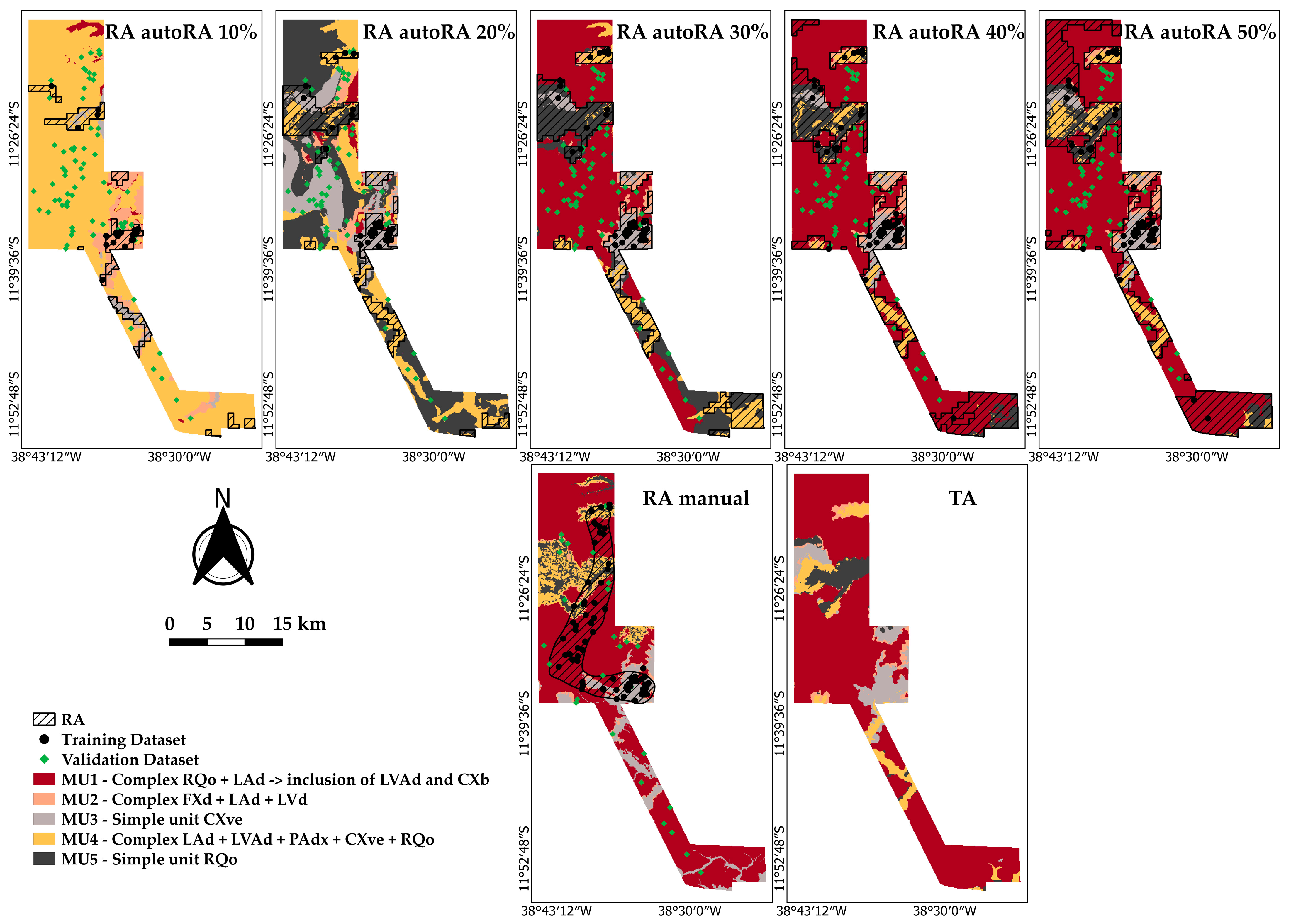
3.4. Soil Maps and Performance

Figure 16 displays the MU maps for Sátiro Dias created by three approaches—RA manual (benchmark), autoRA, and TA—each with respective accuracy and agreement measures (Table 1). The RA manual approach, intentionally adopted during the sampling design survey, achieved 0.75 accuracies and a kappa of 0.50, thus establishing a baseline for comparison with the other methods, autoRA and TA.
The accuracy of the three modeling approaches tested is presented in Table 2. The autoRA method performed poorly at 10% and 20% target areas, with accuracy dropping to around 0.14–0.11 and minimal kappa (0.06–0.01). These low scores highlight that insufficient spatial coverage (only 10–20% of the territory) fails to capture environmental variability, leading to weak model training. However, at 30% coverage, the autoRA-based model displayed a considerable leap in accuracy (0.85) and a moderate kappa (0.42), suggesting that a broader spatial representation bolsters predictive performance by sampling more heterogeneous zones. When coverage reached 40% and 50%, the model attained accuracies of 0.96 (kappa = 0.65 for 40% and 0.49 for 50%), surpassing the RA manual and nearly matching the top performance of the TA approach.
The TA method allocates training/validation sets randomly across the entire domain, yielding an overall accuracy of 0.84 and a kappa of 0.74, with the best splits achieving 0.93 and 0.89, respectively (Figure 17). This indicates that randomly sampling the TA—and repeating splits to stabilize estimates—can generate highly reliable models [23,32].
Nonetheless, autoRA at 30%, 40%, and 50% successfully narrowed the gap. This indicates that a targeted and oriented sampling design considering spatially diverse units can outperform a static RA manual design and challenge the comprehensive TA approach. In particular, 40% autoRA stands out for balancing coverage and modeling success, suggesting that automated, diversity-driven approaches can reduce fieldwork while preserving (and sometimes surpassing) accuracy in this proportional RI-reduced area.
Figure 18 shows the MU frequencies across the training datasets (RA manual, RA autoRA-target areas, and TA), revealing each approach’s strengths and shortcomings. The TA dataset, typical in DSM workflows, relied heavily on MU1 and underrepresented MU2, MU4, and MU5, risking poor model generalization for those classes [65,66,67]. Meanwhile, the RA manual—guided by expert judgment—also concentrates on MU1, indicating potential subjective bias.
In contrast, RA autoRA at higher percentages (40% and 50%) balances MU representation, notably improving the coverage of MU4 and MU5 and reducing MU1’s dominance, thus enhancing reproducibility and scalability. The validation dataset confirmed that RA autoRA consistently encompasses a broader range of units (especially MU3, MU4, and MU5) than the TA or RA manual methods, underscoring its capacity to produce more comprehensive datasets during the training soil sampling design.
The confusion matrix in Table 3 highlights a significant concentration of MU1, demonstrating that autoRA’s optimized sampling distribution provides a superior representation of soil variability compared to the RA manual and TA methods. This is particularly evident when mitigating the overrepresentation of dominant units. When autoRA coverage is low (10–20%), it fails to capture sufficient heterogeneity, resulting in weaker model performance and higher misclassification rates [67,68]. In contrast, increasing autoRA coverage to 30–50% leads to a more even distribution of samples across MUs, enhancing overall model performance by capturing more significant soil heterogeneity and reducing classification errors, especially in underrepresented mapping units. Although the TA method encompasses the full range of RI variability, its overall accuracy does not consistently surpass that of autoRA, suggesting that a selective, diversity-driven approach can be advantageous [69].
Evaluating the RA manual, autoRA, and TA methods reveals MU representation and accuracy differences using the Weighted Producer Accuracy Index (WPAI), Weighted User Accuracy Index (WUAI), and area extension metrics. Under the RA manual approach, MU1 achieves a high User’s Accuracy (0.95) and perfect Producer’s Accuracy, indicating reliable classification in a significant, homogeneous region. The RA manual also included MU3, MU4, and MU5 profiles in the external validation dataset, as shown in the confusion matrix. Specifically, MU3 and MU4 had moderate representation, whereas MU5 exhibited low classification accuracy due to limited validation samples (User’s Accuracy of 0.5 and 0, respectively). The WPAI for MU1 (0.71) further validates the RA manual’s effectiveness in capturing large, consistent MUs while exposing its limitations in addressing variability within smaller classes [70].
Conversely, autoRA’s performance across different sample proportions demonstrates its capability to account for more diverse MU variability. At 10% coverage, high User’s Accuracy (0.95) for MU3 and MU5 indicates the successful detection of dominant variability, supported by a WPAI of 0.76 for MU1. However, the low Producer’s Accuracy for MU5 (0.05) highlights the difficulty in fully representing smaller or more variable units with sparse sampling. Increasing coverage to 20% improves Producer’s Accuracy for MU1 (0.95) and introduces additional MUs (e.g., MU2, MU5) into the validation set, as indicated by a WUAI of 0.59 for MU1 [51]. At 30% coverage, MU1’s User’s Accuracy (0.92) and WPAI (0.59) reflect enhanced classification stability, while coverage levels of 40–50% achieve near-perfect performance for MU1. This underscores autoRA’s increasing reliability when the training set encompasses sufficient variability [71,72].
Figure 19 demonstrates that MU distribution under autoRA 40% coverage is the most balanced among the tested scenarios. For the RA manual method, MU3, MU4, and MU5 were adequately represented in the validation dataset, ensuring balanced external validation. However, with autoRA 40% coverage, MU3, MU4, and MU5 lack validation points in the external validation dataset because their profiles were incorporated into the training dataset. Specifically, for MU5, profiles V9 and PE1004, initially designated for validation, were included in the training. Similarly, for MU4, profile V20 was selected for training, and for MU3, profiles V18 and V3 were also allocated to the training set. Additionally, for MU2, validation profiles V1 and PE1003 were included in the training set by autoRA 40%. This imbalance highlights autoRA’s emphasis on selecting profiles with higher dissimilarity, which shifted specific profiles from validation to training. Meanwhile, the highly sampled MU1 and MU2 were retained in the validation dataset due to their lower dissimilarity scores.
This distribution indicates that while the RA manual method ensured the representation of smaller classes like MU3, MU4, and MU5 in the validation dataset, autoRA prioritized diversity in training, resulting in different trade-offs. The TA method provides a valuable baseline: for MU1, a User’s Accuracy of 1 and a WPAI of 0.84 confirm strong agreement across its extensive distribution (652.88 km2). However, smaller or more variable classes, such as MU3 (User’s Accuracy of 0.7), remain challenging to consistently capture across the domain. While RA manual effectively characterizes large, consistent units, autoRA addresses variability and shows improved performance as sampling proportions increase [73,74]. The WPAI and WUAI indices illustrate how sampling strategies and inherent heterogeneity influence accuracy and reliability. Ultimately, autoRA is distinguished by its ability to accommodate high variability, steadily enhancing performance as the proportion of training samples increases.

3.5. Filling the Research Gap on Automatic Delineation of Reference Area in Digital Soil Mapping

Our findings underscore that autoRA decisively addresses the gap in objective reference area delineation, offering clear practical advantages over manual RA delineation and traditional approaches. By leveraging quantitative environmental covariates to define reference zones, autoRA minimizes subjective bias in site selection [75] and significantly reduces the time and cost associated with soil surveys [8], all while improving sampling efficiency through the more informed targeting of soil variability. This aligns with previous research showing that mapping a small representative area and extrapolating its soil–landscape relationships to similar broader regions can effectively capture soil heterogeneity and serve as a low-cost alternative to full-scale surveys [16].
Moreover, using automated similarity metrics such as Gower’s index to compare environmental conditions between areas provides an objective means to ensure that reference sites encompass the diversity of soil-forming factors, thereby improving the representation of soil variability in digital maps [76]. In Brazil, the adoption of autoRA could have broad impacts on digital soil mapping and environmental planning by expediting initiatives like the PronaSolos national program—saving time, money, and manpower in soil mapping [64]—while ensuring that its implementation aligns with sustainable land management practices. Overall, this study reinforces the importance of autoRA as an innovative tool in digital soil mapping that enhances sampling efficiency and consistency and ultimately supports more informed, sustainable land use decisions.

4. Conclusions

The results underscore the pivotal role of delineating an adequately sized reference area (RA) and ensuring sufficient training points for accurately mapping soil MUs. Applying autoRA based on the highest similarity index values was key to capturing the full range of environmental variability, enhancing the agreement between generated MU maps and the benchmark MU map. As the RA increased from 10% to 50%—and training points grew accordingly—external validation metrics (overall accuracy and index kappa) rose markedly, confirming that broader RA coverage strengthens model performance.
Lower coverage at 10% and 20% yielded insufficient performance (accuracies of 0.14 and 0.11), demonstrating that minimal training data fail to capture environmental complexity. Moving to 30% triggered a step change (accuracy = 0.85, kappa = 0.42), while 40% and 50% produced even higher accuracy (0.96), with 40% offering the best balance (kappa = 0.65). Although the 50% map was also accurate, redundancy in the extensive RA reduced agreement (kappa = 0.49). Meanwhile, manual RA mapping, although moderately effective (accuracy = 0.75, kappa = 0.50), struggled with complex transitions, evidencing the merits of data-driven automation by autoRA.
Comparisons with the total area (TA) approach—where points span the entire study region—indicate that TA can deliver strong results but does not consistently surpass autoRA at 40%. While TA benefits from the broader coverage of the study area, it may also oversample specific features and fail to capture key environmental gradients systematically. In contrast, autoRA strategically pinpoints diverse zones, avoiding redundancy and enhancing modeling performance.
Thus, autoRA emerges as a tool for pre-campaign planning, allowing users to delineate small RAs that encapsulate essential environmental variability and will orient a sampling design with high diversity areas regarding soil forming factors. Specifically, a well-calibrated RA of around 40% proved highly effective, balancing resource demands compared to conventional splitting DSM workflows.

Author Contributions

Conceptualization, M.B.C., H.R., S.G., G.M.V., E.B. and A.L.O.V.; methodology, M.B.C., H.R., S.G., G.M.V. and E.B.; formal analysis, M.B.C., H.R., S.G., G.M.V. and E.B.; investigation, M.B.C., H.R., S.G., G.M.V. and E.B.; resources, M.B.C., H.R., S.G., G.M.V. and E.B.; data curation, M.B.C., H.R., S.G., G.M.V. and E.B.; writing—H.R.; writing—M.B.C., H.R., S.G., G.M.V. and E.B.; visualization, M.B.C., H.R., S.G., G.M.V. and E.B.; supervision, M.B.C., H.R., S.G., G.M.V. and E.B.; project administration, M.B.C., G.M.V., A.L.O.V. and H.R. All authors have read and agreed to the published version of the manuscript.

Funding

This research was funded by Coordenação de Aperfeiçoamento de Pessoal de Nível Superior (CAPES), with a Ph.D. scholarship for the author under the number 161334/2021-0.

Data Availability Statement

The original contributions presented in the study are included in the article, further inquiries can be directed to the corresponding author.

Conflicts of Interest

Author Gustavo Mattos Vasques was employed by the company Brazilian Research Brazilian Agricultural Research Corporation—Soils. The remaining authors declare that the research was conducted in the absence of any commercial or financial relationships that could be construed as a potential conflict of interest.

References

  1. Biswas, A.; Zhang, Y. Sampling Designs for Validating Digital Soil Maps: A Review. Pedosphere 2018, 28, 1–15. [Google Scholar] [CrossRef]
  2. Brus, D.J. Statistical Sampling Approaches for Soil Monitoring. Eur. J. Soil Sci. 2014, 65, 779–791. [Google Scholar] [CrossRef]
  3. Brus, D.J.; Kempen, B.; Heuvelink, G.B.M. Sampling for Validation of Digital Soil Maps. Eur. J. Soil Sci. 2011, 62, 394–407. [Google Scholar] [CrossRef]
  4. Carter, M.R.; Gregorich, E.G. (Eds.) Soil Sampling and Methods of Analysis; CRC Press: Boca Raton, FL, USA, 2007; ISBN 978-0-429-12622-2. [Google Scholar]
  5. Khomutinin, Y.; Fesenko, S.; Levchuk, S.; Zhebrovska, K.; Kashparov, V. Optimising Sampling Strategies for Emergency Response: Soil Sampling. J. Environ. Radioact. 2020, 222, 106344. [Google Scholar] [CrossRef]
  6. Lagacherie, P.; Legros, J.P.; Burrough, P.A. A Soil Survey Procedure Using the Knowledge of Soil Pattern Established on a Previously Mapped Reference Area. Geoderma 1995, 65, 283–301. [Google Scholar] [CrossRef]
  7. Lagacherie, P.; Robbez-Masson, J.M.; Nguyen-The, N.; Barthès, J.P. Mapping of Reference Area Representativity Using a Mathematical Soilscape Distance. Geoderma 2001, 101, 105–118. [Google Scholar] [CrossRef]
  8. de Arruda, G.P.; Demattê, J.A.M.; Chagas, C.d.S.; Fiorio, P.R.; e Souza, A.B.; Fongaro, C.T. Digital Soil Mapping Using Reference Area and Artificial Neural Networks. Sci. Agric. 2016, 73, 266–273. [Google Scholar] [CrossRef]
  9. Mallavan, B.P.; Minasny, B.; McBratney, A.B. Homosoil, a Methodology for Quantitative Extrapolation of Soil Information Across the Globe. In Digital Soil Mapping; Boettinger, J.L., Howell, D.W., Moore, A.C., Hartemink, A.E., Kienast-Brown, S., Eds.; Springer: Dordrecht, The Netherlands, 2010; pp. 137–150. ISBN 978-90-481-8862-8. [Google Scholar]
  10. Voltz, M.; Lagacherie, P.; Louchart, X. Predicting Soil Properties over a Region Using Sample Information from a Mapped Reference Area. Eur. J. Soil Sci. 1997, 48, 19–30. [Google Scholar] [CrossRef]
  11. Ferreira, A.C.d.S.; Ceddia, M.B.; Costa, E.M.; Pinheiro, É.F.M.; do Nascimento, M.M.; Vasques, G.M. Use of Airborne Radar Images and Machine Learning Algorithms to Map Soil Clay, Silt, and Sand Contents in Remote Areas under the Amazon Rainforest. Remote Sens. 2022, 14, 5711. [Google Scholar] [CrossRef]
  12. Ferreira, A.C.S.; Pinheiro, É.F.M.; Costa, E.M.; Ceddia, M.B. Predicting Soil Carbon Stock in Remote Areas of the Central Amazon Region Using Machine Learning Techniques. Geoderma Reg. 2023, 32, e00614. [Google Scholar] [CrossRef]
  13. Lagacherie, P.; Voltz, M. Predicting Soil Properties over a Region Using Sample Information from a Mapped Reference Area and Digital Elevation Data: A Conditional Probability Approach. Geoderma 2000, 97, 187–208. [Google Scholar] [CrossRef]
  14. Lagacherie, P.; Ledreux, C.; Legros, J.-P. Modélisation de la connaissance d’un pédologue cartographe. Mappemonde 1993, 32, 12–13. [Google Scholar] [CrossRef]
  15. Yigini, Y.; Panagos, P. Reference Area Method for Mapping Soil Organic Carbon Content at Regional Scale. Procedia Earth Planet. Sci. 2014, 10, 330–338. [Google Scholar] [CrossRef]
  16. Gonçalves, T.G.; Pons, N.A.D.; Melloni, E.G.P.; Mancini, M.; Curi, N. Digital Soil Mapping: Predicting Soil Classes Distribution in Large Areas Based on Existing Soil Maps from Similar Small Areas. Ciênc. E Agrotecnologia 2021, 45, e007921. [Google Scholar] [CrossRef]
  17. Dornik, A.; Cheţan, M.A.; Drăguţ, L.; Dicu, D.D.; Iliuţă, A. Optimal Scaling of Predictors for Digital Mapping of Soil Properties. Geoderma 2022, 405, 115453. [Google Scholar] [CrossRef]
  18. Grunwald, S. Current State of Digital Soil Mapping and What Is Next. In Digital Soil Mapping: Bridging Research, Environmental Application, and Operation; Boettinger, J.L., Howell, D.W., Moore, A.C., Hartemink, A.E., Kienast-Brown, S., Eds.; Springer: Dordrecht, The Netherlands, 2010; pp. 3–12. ISBN 978-90-481-8863-5. [Google Scholar]
  19. Boettinger, J.L. (Ed.) Digital Soil Mapping: Bridging Research, Environmental Application, and Operation; Progress in soil science; Springer: Dordrecht, The Netherlands; London, UK, 2010; ISBN 978-90-481-8862-8. [Google Scholar]
  20. Horst-Heinen, T.Z.; Dalmolin, R.S.D.; ten Caten, A.; Moura-Bueno, J.M.; Grunwald, S.; Pedron, F.d.A.; Rodrigues, M.F.; Rosin, N.A.; da Silva-Sangoi, D.V. Soil Depth Prediction by Digital Soil Mapping and Its Impact in Pine Forestry Productivity in South Brazil. For. Ecol. Manag. 2021, 488, 118983. [Google Scholar] [CrossRef]
  21. Khaledian, Y.; Miller, B.A. Selecting Appropriate Machine Learning Methods for Digital Soil Mapping. Appl. Math. Model. 2020, 81, 401–418. [Google Scholar] [CrossRef]
  22. Saurette, D.D.; Heck, R.J.; Gillespie, A.W.; Berg, A.A.; Biswas, A. Sample Size Optimization for Digital Soil Mapping: An Empirical Example. Land 2024, 13, 365. [Google Scholar] [CrossRef]
  23. Carvalho, W.D.; Pereira, N.R.; Fernandes, E.I.; Calderano, B.; Pinheiro, H.S.K.; Chagas, C.D.S.; Bhering, S.B.; Pereira, V.R.; Lawall, S. Sample Design Effects on Soil Unit Prediction with Machine: Randomness, Uncertainty, and Majority Map. Rev. Bras. Ciênc. Solo 2020, 44, e0190120. [Google Scholar] [CrossRef]
  24. Casa, R.; Castaldi, F.; Pascucci, S.; Basso, B.; Pignatti, S. Geophysical and Hyperspectral Data Fusion Techniques for In-Field Estimation of Soil Properties. Vadose Zone J. 2013, 12, 1–10. [Google Scholar] [CrossRef]
  25. Grunwald, S.; Vasques, G.M.; Rivero, R.G. Fusion of Soil and Remote Sensing Data to Model Soil Properties. In Advances in Agronomy; Elsevier: Amsterdam, The Netherlands, 2015; Volume 131, pp. 1–109. ISBN 978-0-12-802136-1. [Google Scholar]
  26. Ji, W.; Adamchuk, V.I.; Chen, S.; Mat Su, A.S.; Ismail, A.; Gan, Q.; Shi, Z.; Biswas, A. Simultaneous Measurement of Multiple Soil Properties through Proximal Sensor Data Fusion: A Case Study. Geoderma 2019, 341, 111–128. [Google Scholar] [CrossRef]
  27. Rodrigues, H.; Ceddia, M.B.; Tassinari, W.; Vasques, G.M.; Brandão, Z.N.; Morais, J.P.S.; Oliveira, R.P.; Neves, M.L.; Tavares, S.R.L. Remote and Proximal Sensors Data Fusion: Digital Twins in Irrigation Management Zoning. Sensors 2024, 24, 5742. [Google Scholar] [CrossRef] [PubMed]
  28. Minasny, B.; McBratney, A.B. A Conditioned Latin Hypercube Method for Sampling in the Presence of Ancillary Information. Comput. Geosci. 2006, 32, 1378–1388. [Google Scholar] [CrossRef]
  29. Malone, B.P.; Minansy, B.; Brungard, C. Some Methods to Improve the Utility of Conditioned Latin Hypercube Sampling. PeerJ 2019, 7, e6451. [Google Scholar] [CrossRef]
  30. Saurette, D.D.; Heck, R.J.; Gillespie, A.W.; Berg, A.A.; Biswas, A. Divergence Metrics for Determining Optimal Training Sample Size in Digital Soil Mapping. Geoderma 2023, 436, 116553. [Google Scholar] [CrossRef]
  31. de Carvalho Junior, W.; Saraiva Koenow Pinheiro, H.; Bacis Ceddia, M.; Souza Valladares, G. Pedometrics in Brazil; Springer: Cham, Switzerland, 2024; ISBN 978-3-031-64579-2. [Google Scholar]
  32. McBratney, A.B.; Mendonça Santos, M.L.; Minasny, B. On Digital Soil Mapping. Geoderma 2003, 117, 3–52. [Google Scholar] [CrossRef]
  33. Liaw, A.; Wiener, M. Classification and Regression by randomForest. R News 2002, 2, 18–22. [Google Scholar]
  34. USDA/NRCS. Dynamic Soil Property Guide Version 3; USDA/NRCS: Washington, DC, USA, 2024. [Google Scholar]
  35. Gower, J.C. A General Coefficient of Similarity and Some of Its Properties. Biometrics 1971, 27, 857–871. [Google Scholar] [CrossRef]
  36. Gauld, D.B. Topological Properties of Manifolds. Am. Math. Mon. 1974, 81, 633–636. [Google Scholar] [CrossRef]
  37. Adams, R.A.; Fournier, J.J.F. (Eds.) 4-The Sobolev Imbedding Theorem. In Pure and Applied Mathematics; Sobolev Spaces; Elsevier: Amsterdam, The Netherlands, 2003; Volume 140, pp. 79–134. [Google Scholar]
  38. Ferry, S.; Weinberger, S. Quantitative Algebraic Topology and Lipschitz Homotopy. Proc. Natl. Acad. Sci. USA 2013, 110, 19246–19250. [Google Scholar] [CrossRef]
  39. Falconer, K.J.; Marsh, D.T. On the Lipschitz Equivalence of Cantor Sets. Mathematika 1992, 39, 223–233. [Google Scholar] [CrossRef]
  40. IBGE. Mapeamento de Recurso Naturais do Brasil Escala 1:250.000; Documentação Técnica Geral; Diretoria de Geociências, Coordenação de Recursos Naturais e Estudos Ambientais: Rio de Janeiro, Brazil, 2018. [Google Scholar]
  41. Fick, S.E.; Hijmans, R.J. WorldClim 2: New 1-Km Spatial Resolution Climate Surfaces for Global Land Areas. Int. J. Climatol. 2017, 37, 4302–4315. [Google Scholar] [CrossRef]
  42. Farr, T.G.; Rosen, P.A.; Caro, E.; Crippen, R.; Duren, R.; Hensley, S.; Kobrick, M.; Paller, M.; Rodriguez, E.; Roth, L.; et al. The Shuttle Radar Topography Mission. Rev. Geophys. 2007, 45, RG2004. [Google Scholar] [CrossRef]
  43. Bornand, M.; Favrot, J.C. Cartographie des sols et gestion de l’eau, depuis l’échelle régionale jusqu’a l’échelon parcellaire: L’exemple en France du Languedoc-Roussillon. Bull. Reseau Eros. 1998, 18, 405–418. [Google Scholar]
  44. Favrot, J.C. Pour Une Approche Raisoneé Du Drainage Agricole En France. La Méthode Des Secteurs de Référence. CR Académie Agric. Fr. 1981, 67, 716–723. [Google Scholar]
  45. Favrot, J.-C.; Lagacherie, P. La cartographie automatisee des sols: Une aide a la gestion ecologique des paysages ruraux. Comptes Rendus De L’académie D’agriculture De Fr. 1993, 79, 61–76. [Google Scholar]
  46. Roudier, P.; Hewitt, A.E.; Beaudette, D.E. A Conditioned Latin Hypercube Sampling Algorithm Incorporating Operational Constraints. In Digital Soil Assessments and Beyond; CRC Press: Boca Raton, FL, USA, 2012. [Google Scholar]
  47. Ellili, Y.; Walter, C.; Michot, D.; Pichelin, P.; Lemercier, B. Mapping Soil Organic Carbon Stock Change by Soil Monitoring and Digital Soil Mapping at the Landscape Scale. Geoderma 2019, 351, 1–8. [Google Scholar] [CrossRef]
  48. Keskin, H.; Grunwald, S.; Harris, W.G. Digital Mapping of Soil Carbon Fractions with Machine Learning. Geoderma 2019, 339, 40–58. [Google Scholar] [CrossRef]
  49. Padarian, J.; Minasny, B.; McBratney, A.B. Using Deep Learning for Digital Soil Mapping. SOIL 2019, 5, 79–89. [Google Scholar] [CrossRef]
  50. R Core Team. R: A Language and Environment for Statistical Computing; R Foundation for Statistical Computing: Vienna, Austria, 2024. [Google Scholar]
  51. Costa, E.M.; Ceddia, M.B.; dos Santos, F.N.; Silva, L.d.O.; de Rezende, I.P.T.; Fernandes, D.A.C. Training Pedologist for Soil Mapping: Contextualizing Methods and Its Accuracy Using the Project Pedagogy Approach. Rev. Bras. Ciênc. Solo 2021, 45, 33. [Google Scholar] [CrossRef]
  52. Cheng, X.; Luo, Y.; Xu, X.; Sherry, R.; Zhang, Q. Soil Organic Matter Dynamics in a North America Tallgrass Prairie after 9 Yr of Experimental Warming. Biogeosciences 2011, 8, 1487–1498. [Google Scholar] [CrossRef]
  53. Owens, P.R.; Rutledge, E.M. MORPHOLOGY. In Encyclopedia of Soils in the Environment; Hillel, D., Ed.; Elsevier: Oxford, UK, 2005; pp. 511–520. ISBN 978-0-12-348530-4. [Google Scholar]
  54. Clothier, B.E.; Pollok, J.A.; Scotter, D.R. Mottling in Soil Profiles Containing a Coarse-Textured Horizon. Soil Sci. Soc. Am. J. 1978, 42, 761–763. [Google Scholar] [CrossRef]
  55. Ceddia, M.B.; Villela, A.L.O.; Pinheiro, É.F.M.; Wendroth, O. Spatial Variability of Soil Carbon Stock in the Urucu River Basin, Central Amazon-Brazil. Sci. Total Environ. 2015, 526, 58–69. [Google Scholar] [CrossRef]
  56. da Silva Freitas, L.C.; Cavalcanti, L.C.S.; Neto, J.J.F. Geoenvironmental Diagnosis of the Protected Areas of the Spix’s Macaw, Bahia. Rev. Bras. Geogr. Fis. 2024, 17, 3416–3449. [Google Scholar] [CrossRef]
  57. Silva, M.D.S.D.; Barreto-Garcia, P.A.B.; Monroe, P.H.M.; Pereira, M.G.; Pinto, L.A.D.S.R.; Nunes, M.R. Physically Protected Carbon Stocks in a Brazilian Oxisol under Homogeneous Forest Systems. Geoderma Reg. 2025, 40, e00915. [Google Scholar] [CrossRef]
  58. Junior, P.R.P.R.; Nascimento, F.R.D. Environment, geology-geomorphology and water availability in the Guandu river basin/Rio de Janeiro. William Morris Davis-Rev. Geomorfol. 2022, 3, 1–20. [Google Scholar] [CrossRef]
  59. Gonçalves, R.V.S.; Cardoso, J.C.F.; Oliveira, P.E.; Raymundo, D.; de Oliveira, D.C. The Role of Topography, Climate, Soil and the Surrounding Matrix in the Distribution of Veredas Wetlands in Central Brazil. Wetl. Ecol. Manag. 2022, 30, 1261–1279. [Google Scholar] [CrossRef]
  60. Momoli, R.S.; Cooper, M. Water Erosion on Cultivated Soil and Soil under Riparian Forest. Pesqui. Agropecu. Bras. 2016, 51, 1295–1305. [Google Scholar] [CrossRef]
  61. van Westen, C.J.; Castellanos, E.; Kuriakose, S.L. Spatial Data for Landslide Susceptibility, Hazard, and Vulnerability Assessment: An Overview. Eng. Geol. 2008, 102, 112–131. [Google Scholar] [CrossRef]
  62. Fernandes, K.; Júnior, J.M.; Ribon, A.A.; de Almeida, G.M.; Moitinho, M.R.; de Lima Dias Delarica, D.; Bahia, A.S.R.d.S.; da Silva Oliveira, D.M. Characterization and Detailed Mapping of C by Spectral Sensor for Soils of the Western Plateau of São Paulo. Sci. Rep. 2024, 14, 17311. [Google Scholar] [CrossRef]
  63. Pereira, M.G.; Anjos, L.H.C. Formas extraíveis de ferro em solos do estado do Rio de Janeiro. Rev. Bras. Ciênc. Solo 1999, 23, 371–382. [Google Scholar] [CrossRef]
  64. Costa, E.M.; Rodrigues, H.M.; Ferreira, A.C.D.S.; Ceddia, M.B.; Fernandes, D.A.C. Using Legacy Soil Data to Plan New Data Collection: Study Case of Rio de Janeiro State: Brazil. In Pedometrics in Brazil; De Carvalho Junior, W., Saraiva Koenow Pinheiro, H., Bacis Ceddia, M., Souza Valladares, G., Eds.; Progress in Soil Science; Springer Nature: Cham, Switzerland, 2024; pp. 101–113. ISBN 978-3-031-64578-5. [Google Scholar]
  65. Neyestani, M.; Sarmadian, F.; Jafari, A.; Keshavarzi, A.; Sharififar, A. Digital Mapping of Soil Classes Using Spatial Extrapolation with Imbalanced Data. Geoderma Reg. 2021, 26, e00422. [Google Scholar] [CrossRef]
  66. Baruck, J.; Nestroy, O.; Sartori, G.; Baize, D.; Traidl, R.; Vrščaj, B.; Bräm, E.; Gruber, F.E.; Heinrich, K.; Geitner, C. Soil Classification and Mapping in the Alps: The Current State and Future Challenges. Geoderma 2016, 264, 312–331. [Google Scholar] [CrossRef]
  67. Odgers, N.P.; McBratney, A.B.; Carré, F. Soil Profile Classes. In Pedometrics; McBratney, A.B., Minasny, B., Stockmann, U., Eds.; Springer International Publishing: Cham, Switzerland, 2018; pp. 265–288. ISBN 978-3-319-63439-5. [Google Scholar]
  68. Devine, S.M.; Steenwerth, K.L.; O’Geen, A.T. A Regional Soil Classification Framework to Improve Soil Health Diagnosis and Management. Soil Sci. Soc. Am. J. 2021, 85, 361–378. [Google Scholar] [CrossRef]
  69. Zhang, L.; Zhu, A.-X.; Liu, J.; Ma, T.; Yang, L.; Zhou, C. An Adaptive Uncertainty-Guided Sampling Method for Geospatial Prediction and Its Application in Digital Soil Mapping. Int. J. Geogr. Inf. Sci. 2023, 37, 476–498. [Google Scholar] [CrossRef]
  70. Henrys, P.A.; Mondain-Monval, T.O.; Jarvis, S.G. Adaptive Sampling in Ecology: Key Challenges and Future Opportunities. Methods Ecol. Evol. 2024, 15, 1483–1496. [Google Scholar] [CrossRef]
  71. Huang, J.; McBratney, A.B.; Minasny, B.; Triantafilis, J. Monitoring and Modelling Soil Water Dynamics Using Electromagnetic Conductivity Imaging and the Ensemble Kalman Filter. Geoderma 2017, 285, 76–93. [Google Scholar] [CrossRef]
  72. Gomes, L.C.; Beucher, A.M.; Møller, A.B.; Iversen, B.V.; Børgesen, C.D.; Adetsu, D.V.; Sechu, G.L.; Heckrath, G.J.; Koch, J.; Adhikari, K.; et al. Soil Assessment in Denmark: Towards Soil Functional Mapping and Beyond. Front. Soil Sci. 2023, 3, 1090145. [Google Scholar] [CrossRef]
  73. Zhang, Y.; Saurette, D.D.; Easher, T.H.; Ji, W.; Adamchuk, V.I.; Biswas, A. Comparison of Sampling Designs for Calibrating Digital Soil Maps at Multiple Depths. Pedosphere 2022, 32, 588–601. [Google Scholar] [CrossRef]
  74. Abdulraheem, M.I.; Zhang, W.; Li, S.; Moshayedi, A.J.; Farooque, A.A.; Hu, J. Advancement of Remote Sensing for Soil Measurements and Applications: A Comprehensive Review. Sustainability 2023, 15, 15444. [Google Scholar] [CrossRef]
  75. Zhou, Y.; Biswas, A.; Hong, Y.; Chen, S.; Hu, B.; Shi, Z.; Li, S. Enhancing Soil Profile Analysis with Soil Spectral Libraries and Laboratory Hyperspectral Imaging. Geoderma 2024, 450, 117036. [Google Scholar] [CrossRef]
  76. Khosravani, P.; Baghernejad, M.; Taghizadeh-Mehrjardi, R.; Mousavi, S.R.; Moosavi, A.A.; Fallah Shamsi, S.R.; Shokati, H.; Kebonye, N.M.; Scholten, T. Assessing the Role of Environmental Covariates and Pixel Size in Soil Property Prediction: A Comparative Study of Various Areas in Southwest Iran. Land 2024, 13, 1309. [Google Scholar] [CrossRef]
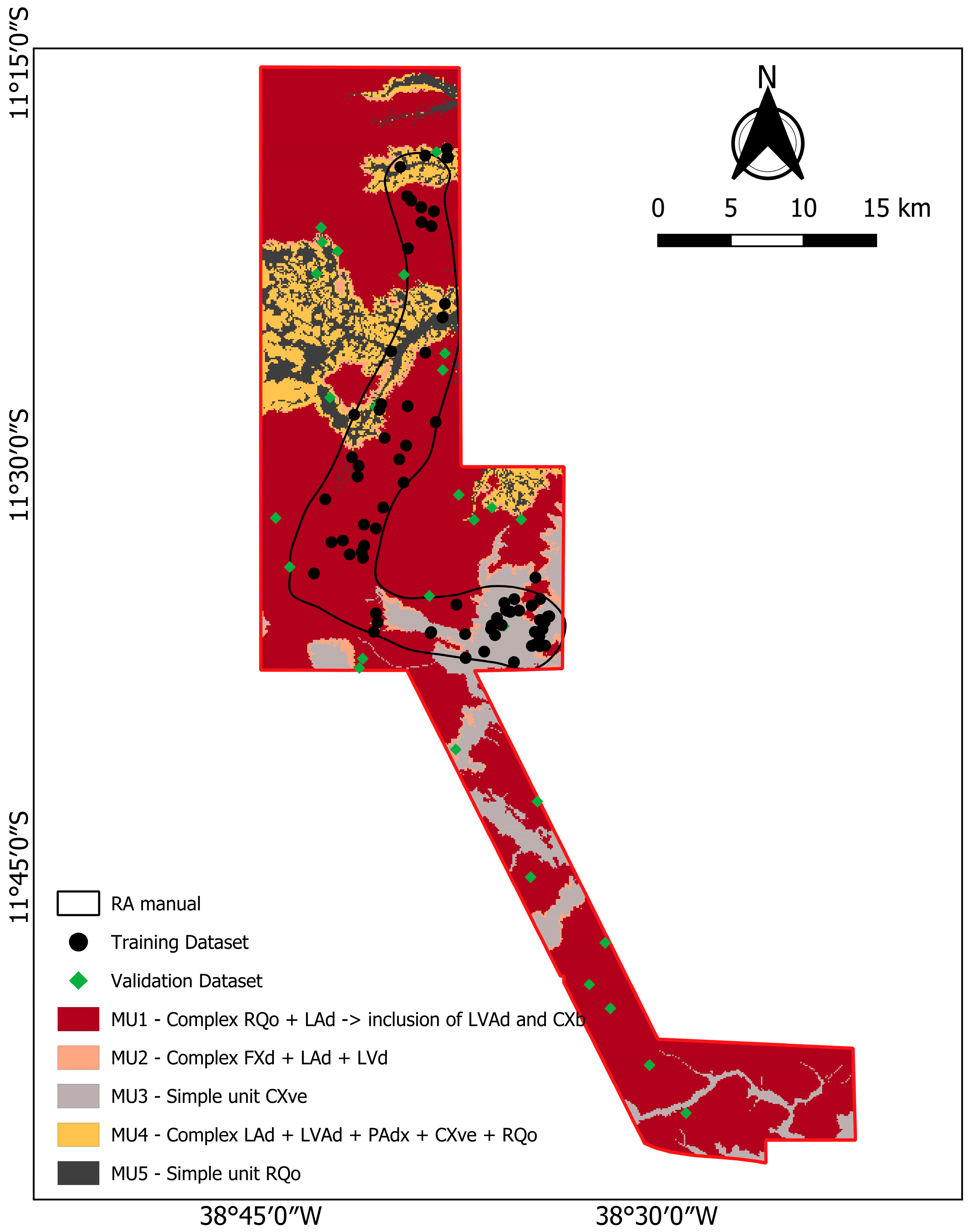
Figure 1. The general workflow of the autoRA algorithm.
Land 14 00604 g001
Figure 2. Location of the study area of Sátiro Dias with the RA manual. A DEM in the background to aid in understanding the physiography of the landscape.
Land 14 00604 g002
Figure 3. Maps of the covariates are used to define the manual RA and automatic RA using the autoRA algorithm. Overview of the research workflow.
Land 14 00604 g003
Figure 4. A flowchart of the methodology implemented in the research compares the RA manual, RA autoRA, and the total area. Characterization of mapping units. (1) RA manual-based models using manually delineated RA samples, (2) RA autoRA-based models from threshold-defined RA autoRA subsets, and (3) TA-based models using the full dataset with repeated 70/30 splits.
Land 14 00604 g004
Figure 5. Map of soil classes in Sátiro Dias developed from soil samples using the RA manual approach used as the benchmark for comparison with the autoRA and the TA approach.
Land 14 00604 g005
Figure 6. Section 1 for explaining the covariates and the soil type described.
Land 14 00604 g006
Figure 7. Section 2 for explaining the covariates and the soil type described.
Land 14 00604 g007
Figure 8. Section 3 for explaining the covariates and the soil type described.
Land 14 00604 g008
Figure 9. Section 4 explains the covariates and the soil type described.
Land 14 00604 g009
Figure 10. Section 5 for explaining the covariates and the soil type described.
Land 14 00604 g010
Figure 11. Section 6 explains the covariates and the soil type described.
Land 14 00604 g011
Figure 12. Section 7 for explaining the covariates and the soil type described.
Land 14 00604 g012
Figure 13. The covariates used in the Gower’s Dissimilarity Index map calculus.
Land 14 00604 g013
Figure 14. Reference areas delineated by autoRA start at 10% of target area coverage concerning the region of interest (RI) with increments of 10% until 50%. The training and validation datasets were reclassified based on the intersection of the outlined RA autoRAs, with the training dataset considered the inner points and the external validation dataset considered the validation points.
Land 14 00604 g014
Figure 15. Graph comparing the capabilities of the autoRA and retrieving the most heterogeneous information of the covariates by representing the pixel frequency at each class/value. (A) Pedology: LAd1, Typic Udults; LAd2, Typic Udults (clayed texture); LVAd, Typic Udults with mixed hematite and goethite; PVAd, Typic Ultisol; PVAe1, Eutrophic Udults on smooth relief; PVAe2, Eutrophic Udults on wave relief; RLd, Lithic Entisols. RQo, Orthic Entisol. (B) Geomorphology: BDP, Buried Degraded Pediplain; HC, Homogeneous Convex; HT, Homogeneous Tabular; HS, Homogeneous Sharp. (C) Gelogy: B, Barreiras Group; M, Marizal Group; FO, Orthogneiss–Migmatite Facies; (D) Average year temperature in °C; (E) DEM, digital elevation model in meters; (F) Average year precipitation in millimeters.
Land 14 00604 g015
Figure 16. Mapping units from the dataset located within the manually delineated reference area (RA). Overlap: RA boundaries dashed, training points in black circles, and external validation points in green lozenges; TA, total area.
Land 14 00604 g016
Figure 17. Variation in the overall accuracy and index kappa results for the 100 sampling seeds splitting to mapping units using the total area (TA) approach.
Land 14 00604 g017
Figure 18. The frequency of MU class on each dataset is used for training and validation.
Land 14 00604 g018
Figure 19. RA autoRA at 40% alongside the corresponding MU map and detailed validation profiles, illustrating their inclusion in the training dataset.
Land 14 00604 g019
Table 1. Soil mapping units in Sátiro Dias.
MUDescriptionEnvironmentArea (km2)%Brazilian Soil Classification SystemUSDA Soil Taxonomy Correspondence
MU1Complex RQo + LAd + CXbdPlateau, flat to gently undulating relief636.9271NEOSSOLO QUARTZARÊNICO Órtico típico, LATOSSOLO AMARELO Distrófico textura média, CAMBISSOLO HÁPLICO Tb Distrófico, textura média-arenosa, A moderadoRQo: Entisols (Typic Quartzipsamments); LAd: Oxisols (Typic Hapludox); CXbd: Inceptisols (Typic Dystrudepts)
MU2Complex FXd + LAd + LVdUpper and middle slopes of plateaus28.493PLINTOSSOLO HÁPLICO Distrófico petroplíntico, LATOSSOLO AMARELO Distrófico petroplíntico, A moderado, fase epipedregoso, Inclusão de LATOSSOLO VERMELHO Distrófico textura médiaFXd: Inceptisols (Aquic Dystrudepts); LAd: Oxisols (Petroplinthic Haplustox); LVd: Oxisols (Typic Hapludox)
MU3Simple unit CXveHills with lower elevation than plateaus (Center of Sátiro Dias)95.4511CAMBISSOLO HÁPLICO Ta Eutrófico típico, textura média-argilosa, Inclusões: LUVISSOLO HÁPLICO Pálico típico, VERTISSOLO HÁPLICO SódicoCXve: Inceptisols (Typic Eutrudepts); Luvisolo: Alfisols (Typic Haplustalfs); Vertissolo: Vertisols (Typic Haplusterts)
MU4Complex LAd + LVAd + PAdx + CXve + RQoHill regions within canyons78.048LATOSSOLO AMARELO Distrófico textura média, LATOSSOLO VERMELHO-AMARELO Distrófico textura média, ARGISSOLO AMARELO Distrófico petroplíntico, CAMBISSOLO HÁPLICO Ta Eutrófico típico, textura média-argilosa, NEOSSOLO QUARTZARÊNICO Órtico típicoLAd: Oxisols (Typic Haplustox); LVAd: Oxisols (Typic Kandiudox); PAdx: Alfisols (Plinthic Kandiustalfs); CXve: Inceptisols (Typic Eutrudepts); RQo: Entisols (Typic Quartzipsamments)
MU5Simple unit RQoLowlands within canyons (north of Sátiro Dias)61.827NEOSSOLO QUARTZARÊNICO Órtico típico, textura muito arenosa, A fracoRQo: Entisols (Typic Quartzipsamments)
TOTAL--900.72100--
Table 2. External validation metrics for each mapping unit map obtained from the different groupings of training data in association with the reference area approach (RA manual and autoRA) method and total area (TA).
N TrainingN ValidationAccuracyKappa
RA manual74280.750.50
RA autoRA 10%22720.140.06
RA autoRA 20%38640.110.01
RA autoRA 30%43590.850.42
RA autoRA 40%51510.960.65
RA autoRA 50%53490.960.49
TA74280.840.74
Table 3. Confusion matrix of RA manual, RA autoRA, and total area (TA).
RA manual
ReferenceMU1MU2MU3MU4MU5TotalUser’s AccuracyArea (km2)WPAIWUAI
MU1190001200.95636.960.710.00
MU2010001128.6
MU30011020.595.29
MU4021*25---78.1
MU50000*0---62.12
Total19321328---
Producer’s Accuracy10.330.500------
AR autoRA 10%
ReferenceMU1MU2MU3MU4MU5TotalUser’s AccuracyArea (km2)WPAIWUAI
MU1*0005353*14.890.760.00
MU20*0000*96.42
MU30070180.9529.79
MU4102*47*746.44
MU51000340.950
Total20906172---
Producer’s Accuracy**0.78*0.05------
AR autoRA 20%
ReferenceMU1MU2MU3MU4MU5TotalUser’s AccuracyArea (km2)WPAIWUAI
MU144181314530.0826.550.030.59
MU21*2115*33.58
MU302*002*193.41
MU40001120.5228.04
MU50000221405.96
Total5620151864---
Producer’s Accuracy0.95**0.070.11------
AR autoRA 30%
ReferenceMU1MU2MU3MU4MU5TotalUser’s AccuracyArea (km2)WPAIWUAI
MU1480004520.92506.480.590.46
MU21100130.3333.18
MU302*002*60.05
MU4000*11*96.09
MU50000111191.74
Total49300759---
Producer’s Accuracy0.980.33**0.14------
AR autoRA 40%
ReferenceMU1MU2MU3MU4MU5TotalUser’s AccuracyArea (km2)WPAIWUAI
MU1480000481637.680.760.22
MU2010001139.57
MU302*002*58.23
MU4000*00*56.95
MU50000*0*95.11
Total48300049---
Producer’s Accuracy10.33***------
AR autoRA 50%
ReferenceMU1MU2MU3MU4MU5TotalUser’s AccuracyArea (km2)WPAIWUAI
MU1470000471631.640.760.00
MU20*0000*43.36
MU302*002*58.95
MU4000*00*78.35
MU50000*0*75.24
Total47200049---
Producer’s Accuracy1****------
Total Area
MU1MU2MU3MU4MU5TotalUser’s AccuracyArea (km2)WPAIWUAI
MU1160000161652.880.840.00
MU20*0000*27.19
MU302701100.7080.9
MU40001120.569.96
MU50001*1*56.61
Total16272229---
Producer’s Accuracy1*10.5*------
* There is no reference class in the validation dataset. The gray background signs the diagonal that represents the correctly classified sample points.
Disclaimer/Publisher’s Note: The statements, opinions and data contained in all publications are solely those of the individual author(s) and contributor(s) and not of MDPI and/or the editor(s). MDPI and/or the editor(s) disclaim responsibility for any injury to people or property resulting from any ideas, methods, instructions or products referred to in the content.

