Integrating Environmental Variables into Geostatistical Interpolation: Enhancing Soil Mapping for the MEDALUS Model in Montenegro

Abstract

Geostatistical methods are important in analyzing natural resources providing input data for complex mathematical models that address environmental processes and their spatial distribution. Ten interpolation methods and one empirical-based classification grounded in empirical knowledge, with a total of 929 soil samples, were used to create the most accurate spatial prediction maps for clay, sand, humus, and soil depth in Montenegro. These analyses serve as a preparatory phase and prioritize the practical application of the obtained results for the implementation and improvement of the MEDALUS model. This model, used to assess sensitivity to land degradation, effectively integrates into broader current and future research. The study emphasizes the importance of incorporating auxiliary variables, such as topography, climate, and vegetation data, enhancing explanatory power and accuracy in delineating the environmental characteristics, ensuring better adaptability to the studied area. The results were validated by the coefficient of determination (R²) and root mean square error (RMSE). For the clay, EBKRP (empirical Bayesian kriging regression prediction) achieved R² = 0.35 and RMSE = 6.95%, for the sand, it achieved R² = 0.34 and RMSE = 17.38%, for the humus, it achieved R² = 0.50 and RMSE = 3.80%, and for the soil depth, it achieved R² = 0.76 and RMSE = 5.36 cm. These results indicate that EBKRP is the optimal method for accurately mapping soil characteristics in future research in Montenegro.

1. Introduction

The age of modern science usually implies the application of geospatial analysis that typically relies on software programs to handle complex data processing and visualization [1]. This is particularly important in studies involving soil characteristics analysis, including both physical and chemical properties. Therefore, advancements in the field of digital soil mapping over the past 20 years have resulted in improving and developing new methods for predicting soil properties [2,3]. Some authors believe that digital soil mapping is a unique aspect of soil science, which Minasny et al. [4] call a “sub-discipline” of soil science, due to the advancements in data collection and processing capabilities. From the earliest stages of digital land mapping [5] to more recent works [6], many authors have written about it; however, this study focuses solely on interpolation techniques. The process involves transforming point data (soil samples) through the interpolation method into processable data, i.e., a continuous surface, applicable to any study area worldwide. According to Meng et al. [7], spatial interpolation is defined as a method used to predict the values of soil properties at unmeasured locations between known sampled locations. In environmental science, accurate interpolation is a crucial part of the field analyses that allows understanding of the variability in soil properties over a given area. Geospatial tools provide useful information for effective land management, crop planning, and environmental conservation in a way that combines diverse and complex databases, improving the quality of the input data and mathematical models’ projections.

Soil mapping research should not only compare and improve interpolation methods but also take into account practical applications. The numerous research findings should be required for better assessment of any sustainable agricultural planning [8,9], land use planning, and resource management [10] applications in precision agriculture [11]. Briefly, these findings should be taken into consideration in any research setting that involves soil properties and environmental variables [12,13]. Additionally, research is justified by providing a data map while reducing cost, time, and effort, utilizing geostatistics as optimal solution for soil analyses [14]. Furthermore, the results of this paper will contribute to the practical goal of this research, which is degradation sensitivity assessment.

Although the interpolation method is frequently used in this field of science, choosing the right method is particularly challenging. The availability of different interpolation methods raises the question of which method is the most accurate. Unfortunately, finding a simple answer to this question is challenging because of the diversity of factors and the large number of spatial variables at play. The main sources of soil data variability are the type of data being interpolated and all soil-forming factors that characterize each specific area [11]. Soil properties differ in factors such as topography, climate, vegetation, hydrology, and parent material [15]. Topography and hydrology are emphasized as major form factors by some authors [16,17,18,19,20], while other authors prioritize vegetation and climate factors [21]. Although these factors can complicate the selection of interpolation methods and prevent uniformity, they can also be incorporated as spatial explanatory information into the prediction process [22]. Topography attributes (elevation, slope, aspect, terrain curvature) are used as explanatory variables for the prediction of soil carbon [22]. Additionally, there are examples of using the hydrological network layout to estimate soil texture [23] and different terrain attributes for soil depth prediction by Hengl et al. [24] and Penížek and Borůvka [25]. When using any model, the methods must be adapted to the study area, as is the case here, in order to find the right interpolation method. Universality does not characterize nature and its processes. There is no exception here: simply reviewing the literature’s numerous methods and their application alone is not enough; instead, a calibration and validation process is required. Therefore, a method that is not widely used (empirical Bayesian kriging regression prediction (EBKRP)), according to our knowledge, has demonstrated why this process is important and necessary. Other methods were selected by reviewing numerous studies in the literature, which are integrated throughout this paper, and the inclusion of a larger number of methods is motivated by the desire not to rule out the possibility that the next method could be the most accurate.

The use of advanced technologies enables the obtainment of auxiliary variables through geographic information systems (GISs), satellite imagery, remote sensing, and machine learning, and data modeling enables better explanation of the variable being interpolated [4,11,25,26,27,28,29]. Machine learning has become one of the most widely used methods by authors as a predictive model for spatial interpolation [3,30,31]. Technology development as stated and the expanding availability of data have probably led to the increased use of machine learning [32] and expanding interest in “data science” [33]. Nevertheless, geostatistical models continue to be valuable as they are better at identifying specific spatial patterns compared to machine learning models [3]. The integration of machine learning and spatial interpolation has produced promising results to date [34]. This comparison was carried out with simple interpolation techniques and has results very similar to the most accurate method. However, according to Padarian et al. [33], advanced methods generally lead to more accurate results than simpler methods. Consequently, this research utilized statistical models and the above-mentioned geospatial technologies to determine soil forming factors and integrate them to accurately define the soil mapping process. Research on soil mapping has rapidly increased to predict soil characteristics at locations where data is unavailable [2,35]. The widespread use of satellite imagery facilitates the identification and analysis of spatial relationships between soil characteristics and environmental data [2,36]. The normalized difference vegetation index (NDVI) is one example of how satellite imagery and remote sensing can be used as an auxiliary variable [27,37,38].

Based on our knowledge, there is only one previous study related to this type of research in Montenegro. However, while the study area is within Montenegro, it covers only 400 km² and focuses on phosphorus interpolation, with the best method achieving a correlation of R² = 0.23 [39].

In this paper, ten interpolation methods were used to estimate the spatial distribution of clay, sand, and humus, and the soil depth. Those are inverse distance weighting method (IDW), ordinary kriging (OK), compositional kriging (COK), universal kriging (UK), geographically weighted regression (GWR), geographically weighted regression kriging (GWRK), spline interpolation (SI), radial basis functions method (RBF), empirical Bayesian kriging (EBK), empirical Bayesian kriging regression prediction (EBKRP), and an experimental method for soil classification grounded in empirical knowledge (empirical-based classification (EBC)). The interpolation parameters in this study were selected based on the potential future application of these interpolated soil characteristics as part of the research on soil degradation processes in Montenegro. This approach ensures that the results of the spatial prediction of the soil characteristics can be effectively integrated into broader and future environmental studies, especially in the context of climate change.

The aim of the study is to determine the most accurate method for the geospatial interpolation of the selected soil parameters (clay, sand, and humus content, soil depth), to provide input data for the implementation and improvement of the MEDALUS (Mediterranean desertification and land use) model to assess soil degradation sensitivity under various climate scenarios for the Montenegro study area. We hypothesize that the inclusion of auxiliary variables improves the soil characteristic interpolation accuracy. Additionally, it is infeasible to universally apply one interpolation method across different study areas, due to the variability in environmental conditions.

2. Materials and Methods

2.1. Study Area

Montenegro is a country in southeastern Europe, located in the western Balkans and covering an area of 13,812 km². It is bordered by Croatia (to the southwest), Bosnia and Herzegovina (to the northwest), Serbia (to the northeast), Albania (to the southeast), and the Adriatic Sea, with a coastline spanning approximately 316 km [40].

The relief in Montenegro is very specific and is characterized by a pronounced geomorphology mostly of mountainous character with small plain areas along the coastline and in the Skadar Lake basin. Supporting this, up to one-third of the entire territory falls into the category of slopes greater than 35%, with nearly another third (30%) falling into the second-steepest slope category of 18% to 35% (

Table 1. (a–d) Empirical-based classification parameters.

(a) Pedology (WBR, 2011)	Area (km2)	Area (%)
Leptosols	6769.9	48.74
Leptic Cambisol	5386.4	38.78
Feralic Cambisol	838.4	6.04
Haplic Gleysol	246.2	1.77
Fluvisol	183.5	1.32
Colluvic Regosol	150.1	1.08
Arenosols	8.5	0.06
Regosols	7.1	0.05
Haplic Planosol	5.7	0.04
Haplic Cambisol	4.9	0.04
Molic Umbrisol	3.1	0.02
Fluvic Cambisol	2.7	0.02
Calcaric	1.5	0.01
Mollic Fluvisol	0.4	0.003
Salt production	0.4	0.003
Histosol	0.2	0.001
Island	0.2	0.001
Haplic Cambisol and Anthrosol	0.1	0.001
Water	280.4	2.02
Settlements	2.5	0.02
(b) CLC Code (2018)	Area (km2)	Area (%)
111	1.8	0.01
112	194.8	1.4
121	16.2	0.1
131	17.3	0.1
141	4.8	0.03
211	7.6	0.1
221	28.6	0.2
231	266.9	1.9
241	1.3	0.0
242	291.4	2.1
243	1629.5	11.7
311	3669.6	26.4
312	986.9	7.1
313	1053.7	7.6
321	1025.0	7.4
322	5.3	0.0
323	109.4	0.8
324	2926.6	21.1
332	167.0	1.2
333	949.9	6.8
334	76.3	0.5
411	108.8	0.8
421	1.0	0.01
(c) Elevation (m)	Area (km2)	Area (%)
<600	2512.7	18.1
600–1200	5967.5	43.0
1200–1800	3447.6	24.8
1800–2400	1950.6	14.1
>2400	0.5	0.004
(d) Slope (%)	Area (km2)	Area (%)
<6	1365.7	9.8
6–18	3723.7	26.8
18–35	4215.7	30.4
>35	4573.7	33.0

d). The northern half of the country is occupied by mountainous terrain, with the highest peak of Zla Kolata in Prokletije, with an altitude of 2534 m.a.s.l. in the eastern part of the country (Figure 1). It is characterized by a Mediterranean climate, defined by warm and somewhat dry summers and moderately cold and fairly wet winters. The proximity of the Adriatic and Mediterranean Seas, alongside the direction of the mountain range and its diversity in altitude and relief, all have an impact on its climate, creating small areas with large differences between the climate of the coast and the climate of the high mountain region, with numerous transitional regional climates between them. The average annual air temperature ranges from 4.6 °C to 15.8 °C from the area of Žabljak, with an altitude of 1450 m, to the coast (0 m). The average annual rainfall ranges from 800 mm to around 5000 mm from the north to the southwest, but for the whole country the average is around 1300 mm, with the formation of snow cover at altitudes above 400 m [41].

According to the Koppen system, Montenegro has two climate classes. The first climate class (C) is characterized by two climate types, Cs and Cf. The Cs is divided into subtypes Csa and Csb, which represent the Mediterranean climate with a hot summer and a variant of the Etesian climate with a warm summer. The Cf has only one subtype, the humid warm temperate climate type (Cfb). The second climate class (D) is characterized by one climate type (Df) and two subtypes, a humid cold temperate climate with a warm summer (Dfb) and a humid boreal climate with a cool summer (Dfc) [42]. According to the Koppen system, three climate types and five subtypes can be found in Montenegro.

The most common type of geological substrate in Montenegro is massive and layered limestones, with dolomites occurring sporadically, accounting for nearly a third of the total country area (32.08%). The dolomites and dolomitic limestones occupy 23.13%, while argillaceous schists, phyllites, sandstones, conglomerates, sporadically with limestones and conglomerates, sandstones, breccia, shales, marls, and marly limestones occupy about 12% each. Other types of geological substrates individually occupy less than 6% of the territory. Leptosols are the most common soil type in the country, with 48.74%, followed by Leptic Cambisol (38.78%) and Feralic Cambisol (6%). Each of the other soil types accounts for less than 2% of the country’s territory (WBR 2011) (Figure 2, Table 1a). Rendzina soils (Leptosols, 48.74%) are rich in humus and typically shallow developing from carbonate or sulfate-rich parent material. They are predominantly found in mountainous regions, where they form on loose substrates with a high proportion of skeletal material. Brow soils (Leptic Cambisol, 38.78%) are generally described as having moderate fertility (low fertility in highlands and higher fertility in valleys), a strong dependence on parent material with significant skeletoid profile, and geographical distribution across specific regions, with variations in soil depth [43]. Montenegro is characterized by shallow soils with low fertility potential and, therefore, limited suitability for plant development [44]. According to Fuštić and Đuretić [43], there are five categories of soil fertility. Soils with high fertility (I and II) occupy only 1.5% of the country’s territory, while those with medium fertility (III and IV) cover 4.3%. Soils with limited fertility (V and VI) occupy a quarter of the territory, whereas low-fertility soils account for 46.2% (VII and VIII), and infertile soils make up as much as 22.7%. The limited availability of soil as a resource, or rather its low fertility, where the first two categories, high and medium fertility, occupy only 5.8% of the territory, raises the issue of protecting this important resource from further degradation. The Land Use Land Cover (LULC) classes for the country of Montenegro were derived from the CORINE Land Cover (CLC) database (2018), which provides comprehensive land cover information at a scale of 1:100,000, with the CLC codes given in the parentheses. Broad-leaved forest (311) occupies 3669.6 km², which is 26.44% of the country’s total area, followed by transitional woodland–shrub (324) at 21.09%. Agriculture occupies the majority of the land, with natural vegetation (243) occupying 11.74%, natural grasslands (321), coniferous forest (312), and sparsely vegetated areas (333) each occupying around 7% (Table 1b).

2.2. Soil Sampling and Analysis

For the purposes of this paper, samples from the book “Soils of Montenegro” were digitized as primary soil samples. This book contains detailed physical and chemical analyses of the soil samples, the data collected for pedogenetic studies, and the creation of a pedological map of Montenegro on a scale of 1:50,000, whose creation took from 1965 to 1988 (Figure 2) [43].

Establishing a database with 929 samples required a significant amount of work. Finding accurate locations and digitizing sampling sites, entering the measured values into numerous tables, and transforming and combining all the data to form a spatial database in GIS were the required steps. The samples represent soil profiles whose characteristics are measured by soil horizons. The Kocman method was used to determine the humus content, and the granulometric composition was classified using Atterberg’s limit values and Stokes’ law of free settling in water.

A total of 929 soil samples of clay, sand, humus, and depth were digitized. The rest of text I agree with. For the soil depth, to the primary soil samples (929), samples identified as bare rock (soil depth 0 cm) were added. They could not be included in the original group of samples because there was no soil that could be sampled and analyzed to create a pedological map. Therefore, remote sensing data were used in combination with CORINE Land Cover (CLC 2018) to create a completed group of samples for determining the soil depth, resulting in an additional 1864 samples from the bare land category (CLC code 332 and 333, certified with remote sensing data), with a soil depth of 0 cm (Figure 2). According to the CORINE definition and classification, these two classes (332 and 333) fall into the category of very shallow soil (a few cm) or no soil at all. The samples of clay, sand, and humus (929 soil samples) were taken as weighted averages for a depth of 0–20 cm.

As previously stated, the parameters were selected with the intention of describing and evaluating the degradation process, and thus their sampling depth was chosen. Soil degradation primarily affects the removal of topsoil from the land surface [45,46]. The substantial impact of the destructive effect of the degradation process occurs in the surface layer and restricts important soil processes and the formation of vegetation cover [47]. Most of the root density is located in topsoil and therefore interacts with degradation processes [48]. Soils in Montenegro are shallow, and since rendzines are characterized as “humus-rich shallow soils” that occupy nearly half of the country [44], the sampling depth in this study was selected (weighted averages 0–20 cm). The soil depth parameter is interpolated without alteration, as this parameter affects the soil’s characteristics.

To assess the spatial distribution of the samples, we used a Moran’s I test and obtained results for all the soil properties—clay, sand, humus, and soil depth—confirming their clustered nature. The Moran’s I values ranged from 0.435 to 1.034, the Z-scores were between 1.796 and 4.211, and the p-values ranged from 0.072 to 0.000025. This outcome is expected, given the large number of samples and the presence of many closely spaced sample points with logically similar characteristics.

2.3. Geostatistical Analysis and Interpolation Methods

All the data and interpolation methods utilized for this paper were processed using the GIS software packages ArcMAP (v.10.7.1.) and ArcGIS Pro (v. 3.2.2.) in conjunction. A total of ten interpolation methods and an empirical approach were used as the experimental classification method in order to compare their performance and determine the most suitable method for interpolating soil characteristics in Montenegro. The selection of these methods results from a review of numerous previous applications in similar studies, their relevance to soil property mapping, and, in some cases, their relevance to computational efficiency [27,29,49,50,51,52,53,54]. Additionally, the interpolation methods were chosen for their practical application; therefore, methods that can be applied in ArcMAP and ArcGIS Pro were selected. Cross-validation was performed as an integrated process that is included when using the ArcMAP (v.10.7.1.) and ArcGIS Pro (v. 3.2.2.) software. This feature belongs to the Geostatistical Analyst tool in the ArcMAP (v.10.7.1.) software. Straightforward interpolations such as IDW and kriging variants, etc. were used to compare the bases for more “complex” time-consuming methods (e.g., EBKRP, GWRK). Their complexity is reflected in the multi-stage calculation process and the ability to incorporate auxiliary variables, which improves prediction accuracy. The application of EBKRP is less common than the other methods. The following methods were used:

• Inverse distance weighting method (IDW);
• Ordinary kriging (OK);
• Compositional kriging (COK);
• Universal kriging (UK);
• Geographically weighted regression (GWR);
• Geographically weighted regression kriging (GWRK);
• Spline interpolation (SI);
• Radial basis functions method (RBF);
• Empirical Bayesian kriging (EBK);
• Empirical Bayesian kriging regression prediction (EBKRP);
• Empirical-based classification (EBC).

2.3.1. Inverse Distance Weighting Method (IDW)

The basic principle behind the IDW spatial interpolation method is that values are estimated by assigning weights to the input samples based on their distances to the predicted location [55,56]. This deterministic method assigns a weighted average inversely proportional to the distance from each input sample to the predicted location [57]. The easy calculation and application of this method also have limitations. When the sampling location has an uneven distribution, the method may produce inaccurate results [7]. Equal weights are assigned to input points within the specified radius, which can unduly influence the interpolated values through outliers or erroneous data [58]. The selection of a power parameter whose influence decreases with distance significantly affects the accuracy of the results [59].

2.3.2. Ordinary Kriging (OK)

Ordinary kriging, as one of the fundamental techniques in the field [60], is also among the most widely utilized interpolation methods [27,29]. Kriging, a geostatistical method, utilizes observed values and their spatial arrangement to estimate values at unsampled locations by computing a weighted average of neighboring points within a defined area [52,61]. In general, the OK method is susceptible to outliers and the density of sampling points, leading to some biased estimates and reduced accuracy in heterogeneous environments [27,59].

2.3.3. Compositional Kriging (COK)

Compositional kriging is a geostatistical technique that endeavors to enhance interpolation precision by incorporating additional auxiliary variables [52,62]. Improving estimation accuracy by utilizing the strong spatial correlation between primary variables and auxiliary variables [63,64] to estimate the values at unsampled locations. In this study, simple cokriging outperforms the commonly used ordinary cokriging.

2.3.4. Universal Kriging (UK)

Universal kriging incorporates a polynomial function of spatial locations into its methodology [62]. This is particularly useful when there is a discernible surface trend in the data, as the polynomial function helps capture and model this trend effectively [7]. This approach estimates values at unsampled locations while considering systematic spatial variation beyond the observed data’s captured variability [65].

2.3.5. Geographically Weighted Regression (GWR)

Geographically weighted regression is a statistical technique developed with an emphasized application to the relationships between variables that spatially change [66]. This variation and the acknowledgment that relationships between parameters can spatially differ across the study area mean that GWR provides flexible estimations of observations [51,67]. The GWR method implies a multiple linear regression model between a target variable and explanatory variables that expands upon the conventional linear regression model to handle non-stationary relationships [27,68]. The prediction for unsampled locations incorporates a distance decay function using a weighted matrix to accommodate the nonuniformity of the study area [66,67].

2.3.6. Geographically Weighted Regression Kriging (GWRK)

Geographically weighted regression kriging combines aspects of the GWR and kriging methods, thereby expanding upon GWR’s capabilities. GWRK involves two distinct components: the deterministic component, first simulated by the GWR model to predict trends from the target variable and auxiliary variables [27], and the stochastic component, where residuals are kriged and added to the trend estimates [51].

2.3.7. Spline Interpolation (SI)

Spline interpolation functions by describing segments of a line or surface that are fitted together to form a smooth representation of the data. These segments are composed of polynomials [11]. Spline interpolation is especially useful for irregularly spaced sampled locations [69], as well as for surfaces with gentle variations [70]. Potential sources of error may occur when extrapolating beyond the range of known sampled locations [71] and when there are significant fluctuations in surface values over a short horizontal span [70].

2.3.8. Radial Basis Functions Method (RBF)

In essence, RBF as a deterministic method is concisely explained by the authors Meng et al. [7], who said that “RBF can be defined as a weighted sum of translations of a radial symmetric function augmented by a polynomial term”. Unlike the IDW method, this method provides accurate approximations when sampling locations are irregularly spatially spaced [72,73], and which consist of a substantial number of data points and minimal variability [27].

2.3.9. Empirical Bayesian Kriging (EBK)

Empirical Bayesian kriging is a geostatistical interpolation method based on the kriging method that utilizes a Bayesian framework to enhance the accuracy of spatial predictions by generating numerous semivariograms from the provided data, taking into account the uncertainty in estimating the semivariogram [74]. EBK can effectively predict spatial datasets with variations or changes in statistical properties across the study area [75]. However, limitations arise when working with large datasets because the estimation of the variogram parameters relies on restricted maximum likelihood, which imposes constraints [74].

2.3.10. Empirical Bayesian Kriging Regression Prediction (EBKRP)

Empirical Bayesian kriging regression prediction combines empirical Bayesian kriging (EBK) with auxiliary variables that have a strong correlation with the data being interpolated [54]. Regarding this, the advancement in geostatistical interpolation results from the combination of kriging with regression analysis [76]. EBKRP combines EBK interpolation with least squares regression, leveraging additional explanatory variables to enhance spatial predictions and addressing multicollinearity through Principal Components Analysis (PCA) [54,76].

2.3.11. Empirical-Based Classification (EBC)

This method was developed for the purpose of this study. It is based on experience and knowledge of one of the primary soil formation variables that can be overlapped and used to determine the spatial distribution of the soil parameter. For this method, the soil type was used as a primary factor, with the general characteristics of a soil type identified (pedological map) (Figure 2). Further, parameter combinations were added, including elevation, slope, aspect, and CLC. The elevation, slope, and aspect were derived from a digital elevation model (DEM) in 30 × 30 m resolution [77]. The intersections between the soil property layers formed clusters, from which the average values of the clay, sand, humus, and soil depth parameters were computed. These values were then assigned to polygons within the same cluster type that lacked direct field observations (Figure 3).

The best results, in the form of the best combination of parameters, were soil type, elevation, and slope for the clay, sand, and soil depth, while soil type, elevation, and CLC (2018) were the best combination for the humus, as determined by the validation methods coefficient of determination (R²) and root mean square error (RMSE), which is explained in detail in the Results and Discussion sections. Many parameters were used. Those that gave the best results are shown in Table 1.

2.4. Auxiliary Variables

Achieving a more precise determination of the interpolated soil characteristics in this paper, such as depth and clay, sand, and humus content, can pose significant challenges, especially in regions with complex geomorphological and climatological features. The pronounced relief of Montenegro, which is characterized by significant topographic variations over short distances and the presence of a diverse climate from the north to the south, emphasizes the necessity of integrating auxiliary variables such as relief (slope, TWI, and plan curvature), climate (air temperature, precipitation), and NDVI. Interpolation techniques are utilized to incorporate additional variables, increasing the explanatory power and accuracy in delineating the characteristics of the study area. These auxiliary variables are directly or indirectly associated with the values being interpolated.

The auxiliary variables used in this paper (

Table 2. Summary table of the implemented auxiliary variables.

			Clay	Sand	Humus	Depth
Number of soil samples		Interpolation	829	829	829	2613
		Validation	100	100	100	180
			auxiliary variables
Interpolation method	IDW		/	/	/	/
	OK		/	/	/	/
	COK		R	slope	DEM	NDVI
	UK		/	/	/	/
	GWR		TWI, R, T *	DEM *, slope, NDVI	DEM *, slope, NDVI, R	DEM, slope, NDVI *, TWI, R, and plan curvature
	GWRK		TWI, R, T *	DEM *, slope, NDVI	DEM *, slope, NDVI, R	DEM, slope, NDVI *, TWI, R, and plan curvature
	SI		/	/	/	/
	RBF		/	/	/	/
	EBK		/	/	/	/
	EBKRP		TWI, R, T *	DEM *, slope, NDVI	DEM *, slope, NDVI, R	DEM, slope, NDVI *, TWI, R, and plan curvature
	EBC		soil type, DEM, slope	soil type, DEM, slope	soil type, DEM, CLC	soil type, DEM, slope

* The auxiliary variables with the highest individual explanatory power.

) are topographic factors derived from a digital elevation model (DEM) with a 30 × 30 m resolution, including terrain slope, terrain wetness index (TWI), and curvature of terrain (plan curvature) [14,28,77,78]. It is well-established that relief factors have a significant influence on soil formation, like elevation and slope [79]. The TWI quantifies moisture availability according to the topographic features of the study area [80], whereas the plan curvature indicates the soil sensitivity to erosion, i.e., changes in soil properties, as determined by the degree of the terrain surface curvature [81,82].

Previous authors [20,83,84] support the use of geostatistical analysis with topographical factors as auxiliary variables to improve the accuracy of interpolated soil properties. Remote sensing data were used to obtain a normalized difference vegetation index (NDVI) as an additional auxiliary variable with the same 30 × 30 m resolution [77,85], by using Equation (1):

$$\mathrm{N}\mathrm{D}\mathrm{V}\mathrm{I}={\displaystyle \frac{{\mathrm{B}\mathrm{a}\mathrm{n}\mathrm{d}}_5-{\mathrm{B}\mathrm{a}\mathrm{n}\mathrm{d}}_4}{{\mathrm{B}\mathrm{a}\mathrm{n}\mathrm{d}}_5+{\mathrm{B}\mathrm{a}\mathrm{n}\mathrm{d}}_4}}$$

(1)

where Band₄ and Band₅ correspond to red and near-infrared (NIR) in the Landsat 9 satellite images (LC09_L2SP_187030_20230719_20230802_02_T1 and LC09_L2SP_186031_20230728_20230802_02_T1).

Temperature (T), precipitation (R), and vegetation exert significant influence on soil formation, operating through various mechanisms and processes [86,87,88]. This study used annual average temperature and rainfall data for 21 years (2000–2020) [41].

To select appropriate explanatory variables for a better understanding of both the interpolation method and the soil characteristics being interpolated, ordinary least squares (OLS) regression was performed. This involved testing numerous parameters to establish connections between the soil characteristics and auxiliary variables (over 12), and only those with high statistical significance are utilized in the interpolation process in this paper. The interpolation methods that use auxiliary variables are COK, GWR, GWRK, and EBKRP (Table 2).

2.5. Validation Methods

The prediction accuracy of the soil characteristics is determined by comparing the actual measured values with the predicted values obtained through interpolation. The data accuracy is compared using Pearson’s correlation (r) and coefficient of determination (R²) (Equation (2)) as well as the root mean square error (RMSE) between datasets (Equation (3)):

$$R^2=1-{\displaystyle \frac{{\sum }_1^n{(y_i-{\widehat{y}}_i)}^2}{{\sum }_1^n{(y_i-{\overline{y}}_i)}^2}}$$

(2)

$$RMSE=\sqrt{{\displaystyle \frac{1}{n}}\sum _{i=1}^n{(y_i-{\widehat{y}}_i)}^2}$$

(3)

The validation process of the interpolation methods for soil characteristics is considered confirmatory [89]. A higher R² indicates a stronger correlation between the interpolated and actual values, while a lower RMSE indicates reduced error, both indicating improved model performance, as seen in many studies [7,11,27,29].

From a total of 929 soil samples of clay, sand, humus, and depth 100 samples were initially separated for validation, and interpolation methods were implemented with 829 soil samples. For the soil depth, an additional 1864 samples, recognized as bare rock (soil depth 0 cm), were used for interpolation, of which 80 samples were separated for validation. This brings the total number of interpolation samples to 2613, with 180 used for validation. The reason for using 80 additional soil depth samples is that the areas identified through satellite imagery, combined with the CLC data, reveal clusters of bare rock surfaces. As a result, each validation sample point can accurately represent the entire rocky surface. The sample points for validation were selected randomly using ArcMAP (using tool subset features). All the samples were obtained from the research presented in the book by Fuštić and Đuretić [43].

3. Results

Four parameters, clay, sand, and humus content and soil depth, were analyzed and determined using the ten interpolation methods to identify the most accurate method suitable for the study area of Montenegro, as well as an experimental soil classification method based on empirical knowledge.

Pearson correlation analysis was used to assess the degree of connections among the soil characteristics and auxiliary variables. Only those with high statistical significance (p-value < 0.01) were included. For the interpolation of clay, the parameters TWI, R, and T were used, explaining approximately 10% of the variability (R² = 0.1). The same result was obtained for the sand, although with different parameters (DEM, slope, and NDVI). The parameters DEM, slope, NDVI, and R were utilized to explain the humus variability, accounting for approximately 20% of the variability (R² = 0.2). The interpolation of soil depth with the parameters DEM, slope, NDVI, TWI, R, and plan curvature resulted in the highest coefficient of determination (R² = 0.3)

The correlation results show relationships not only between the auxiliary variables and soil characteristics but also within the auxiliary variables themselves. In order to mitigate the multicollinearity issue, diagnostics were conducted on the ordinary least squares (OLS) regression model, indicating redundancy among some explanatory variables. Based on the results, appropriate steps were taken, such as removing highly correlated variables. A set of parameters that best describes the individual soil characteristics was selected. Consequently, a combination of parameters that best describes the individual soil characteristics was selected, as shown in Table 2.

3.1. Descriptive Statistics

The analysis of the soil characteristics reveals significant variability across the samples (

Table 3. Descriptive analysis of measured soil characteristics in Montenegro.

Soil Characteristics	Min	Max	Mean	Standard Deviation
Clay (%)	0	51.0	9.6	7.4
Sand (%)	0	89.3	32.6	20.3
Humus (%)	0.1	43.6	5.4	5.4
Depth (cm)	0	160.0	15.7	28.4

). The clay content varied from 0 to 51%, with an arithmetical mean of 9.6% and a standard deviation of 7.4%. The sand content exhibited a broader range, spanning 0.0 to 89.3%, with an arithmetical mean of 32.6% and a standard deviation of 20.3%. The humus content showed a range from 0.1 to 43.6%, with an arithmetical mean value of 5.4% and a standard deviation of 5.4%. The soil depth varied from 0.0 to 160 cm, with an average depth of 15.7 cm and a standard deviation of 28.4 cm. In summary, the soil properties showed diverse characteristics with substantial variability, particularly in the sand content and soil depth, which is expected, considering that the samples represent the entire country of Montenegro.

3.2. Comparative Analysis of Different Interpolation Methods

To evaluate the accuracy of the interpolation method, we utilized the coefficient of determination (R²) and the root mean square error (RMSE) (

Table 4. Prediction accuracy results of soil characteristics using coefficient of determination (R²) and RMSE as comparison criteria.

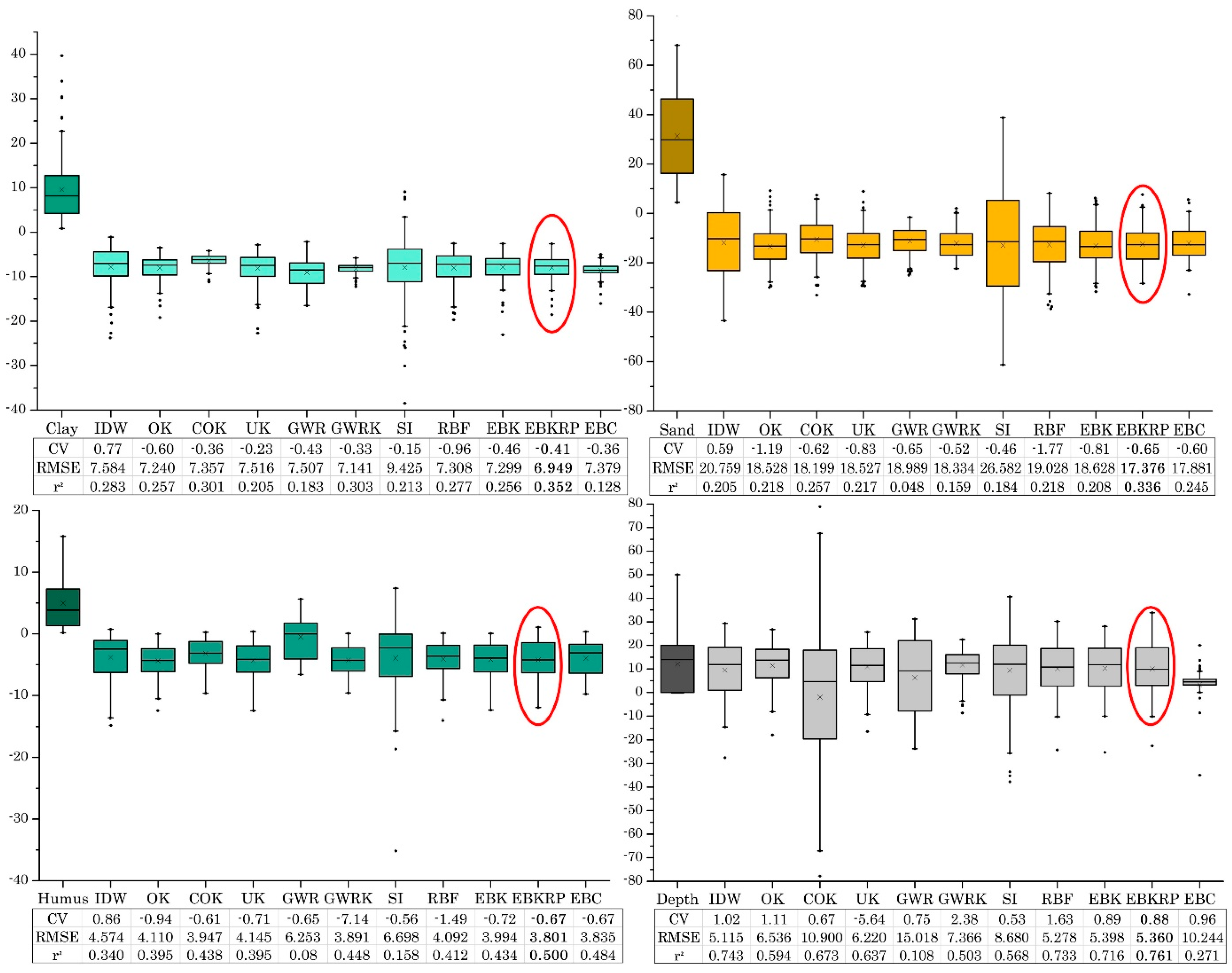
		Clay		Sand		Humus		Depth
		R2	RMSE	R2	RMSE	R2	RMSE	R2	RMSE
Interpolation method	IDW	0.283	7.584	0.205	20.759	0.340	4.574	0.743	5.115
	OK	0.257	7.240	0.218	18.528	0.395	4.110	0.594	6.536
	COK	0.301	7.357	0.257	18.199	0.438	3.947	0.673	10.9
	UK	0.205	7.516	0.217	18.527	0.395	4.145	0.637	6.220
	GWR	0.183	7.507	0.048	18.989	0.080	6.253	0.108	15.018
	GWRK	0.303	7.141	0.159	18.334	0.448	3.891	0.503	7.366
	SI	0.213	9.425	0.184	26.582	0.158	6.698	0.568	8.680
	RBF	0.277	7.308	0.218	19.028	0.412	4.092	0.733	5.278
	EBK	0.256	7.299	0.208	18.628	0.434	3.994	0.716	5.398
	EBKRP	0.352	6.949	0.336	17.376	0.500	3.801	0.761	5.360
	EBC	0.128	7.379	0.245	17.881	0.484	3.835	0.271	10.244

Values with highest R² and lowest RMSE.

).

For the clay interpolation method assessment, EBKRP has the highest determination coefficient (R² = 0.352) and the lowest RMSE of 6.948. GWRK has the second highest coefficient of determination of R² = 0.303 and an RMSE of 7.140, which is slightly better than COK with R² = 0.301 and an RMSE of 7.357. The IDW method has a determination coefficient of R² = 0.283, which is 0.006 better than the RBF coefficient (R² = 0.277) but has a lower RMSE of 7.308. The OK and EBK methods have a better RMSE of 7.24 and 7.299 than IDW and RBF, but a lower determination coefficient, with similar values to the third decimal place, R² = 0.257 and R² = 0.256 for EBK. The UK method has R² = 0.205 and an RMSE of 7.516. The interpolation method with the highest root mean square error is SI (9.425) with a determination coefficient of R² = 0.213, and the GWR method had the lowest R² = 0.183 and an RMSE of 7.507 (Figure 4, Table 4).

The interpolation method evaluation for the sand indicates that the most accurate method is EBKRP, with R² = 0.336 and an RMSE of 17.376. The COK method has a determination coefficient of R² = 0.257 and an RMSE of 18.199 as the second-best score, with a significant gap with the determination coefficient from EBKRP. OK and RBF have the same determination coefficient of R² = 0.218 and RMSE values of 18.528 and 19.028. UK has similar values to OK and RBF of R² = 0.217 and an RMSE of 18.527. Similarly, the EBK and IDW methods have almost the same results for the determination coefficient, R² = 0.208 and R² = 0.205 with RMSE values of 18,628 and 20,759. SI has R² = 0.184 and the worst result for the RMSE (26.582). The determination coefficient (R²) of the GWRK method is 0.159 and with an RMSE of 18.334 and GWR has the lowest determination coefficient (R² = 0.048) and a similar RMSE to GWRK, of 18.989 (Figure 4, Table 4).

For the humus, the EBKRP method has a value of R² = 0.500 and an RMSE of 3.801, which indicates that is the most accurate interpolation method for this soil characteristic. The GWRK, COK, and EBK methods have similar determination coefficients R² = (0.448, 0.438, 0.434) and also similar RMSE values of 3.891, 3.947, and 3.994. RBF has R² = 0.412 and an RMSE of 4.092. The UK and OK methods have the same coefficient of determination (R² = 0.395) and roughly the same RMSE values of 4.145 and 4.110. The determination coefficient of R² = 0.340 and RMSE of 4.574 correspond to the IDW method. SI has R² = 0.158 and the highest RMSE of 6.98, and the GWR method, as in the interpolation of the clay and sand, has the lowest determination coefficient (R² = 0.080) and an RMSE of 6.253. (Figure 4, Table 4).

For the soil depth, the top three methods after validation that prove to be the most accurate are EBKRP (R² = 0.761), IDW (R² = 0.743), and RBF (R² = 0.733) with the following RMSE values: EBKRP (5.360), IDW (5.115), and RBF (5.278). Immediately following this set of values is the EBK method, with R² = 0.716 and an RMSE of 5.398. The COK method has a value of R² = 0.673 and an RMSE of 10.9. The UK method has a determination coefficient of R² = 0.647 and an RMSE of 6.220, with similar results to OK with R² = 0.594 and an RMSE value of 6.536. SI has a higher determination coefficient than GWRK (R² = 0.568 > R² = 0.503) and a higher RMSE value (SI (8.680) > GWRK (7.366)), which has the opposite meaning compared to the determination coefficient. The method with the lowest determination coefficient and highest root mean square error is GWR (R² = 0.108 and RMSE = 15.018) (Figure 4, Table 4).

The results for EBC classification are separate because it is not a classical interpolation method, although the outcome is the same in determining the soil characteristics’ spatial distribution. For the clay, the EBC method has a value of R² = 0.128 and an RMSE of 7.379. For the sand, the results improve, with a value of R² = 0.245 and an RMSE of 17.881. The humus has the most accurate results, with R² = 0.484 and an RMSE of 3.835. For the soil depth, the EBC method has a value of R² = 0.271 and an RMSE of 10.244.

4. Discussion

While there are numerous scientific papers on interpolation and related topics, there is no definitive answer that defines a single method universally applicable even for a specific parameter across different study areas. The selection of the best method for a study area involves the consideration of multiple variables, necessitating the determination of the most suitable method for specific environmental circumstances and variables. These circumstances relate to many applied methods but no matching parameters [27]; conversely, the parameters are the same (depth) but not environmentally the same, with a majority of agricultural land and relatively flat land, which, compared to Montenegro, is the complete opposite in Penížek and Borůvka [25].

For humus interpolation, there are similar parameters as in carbon (C) interpolation in Ref. [37], which studied an area with comparable geomorphology but within a small watershed of only 8.05 km². There are various studies on texture interpolation [50,52,90,91] but according to this paper, the most accurate method differs from those used in previous studies. The EBKRP was not even considered in those papers. Therefore, there is always a necessity to determine the optimal method for the study area’s specific environmental conditions and the variables being interpolated. Overall, the interpolation parameters in this study were selected to support future research on soil degradation processes in Montenegro. Therefore, the spatial prediction results are relevant for the current analysis and can be effectively integrated into broader ongoing and future environmental studies.

The obtained and analyzed results show that the EBKRP method provides the most accurate interpolation for all the soil characteristics data in this study area. Although some interpolation methods have debatably close predictions, such as the IDW method’s prediction of soil depth [91], the EBKRP method consistently performs better across all four soil parameters. Additional comparative results are presented in Table 4. It is interesting that there are not many studies applying this method, as is the case with other methods from the study, yet the EBKRP method is considerably more accurate for soil characteristics other than soil depth. This may be attributed to the inclusion of auxiliary variables that better define the study area [25,54]. The soil depth was more accurately interpolated across all the methods, particularly those incorporating the additional variables, due to the clearer relationship of auxiliary variables such as slope, DEM, TWI, and plan curvature compared to the auxiliary variables’ relationship with the clay, sand, and humus, which is confirmed by correlation. Especially in Montenegro, the variables that better define complex geomorphological features from mountainous regions to coastal regions, with large variations in elevation and terrain slopes, sudden changes occur that can also be difficult for the methods to recognize. All of this is accompanied by the climate conditions that characterize the region. This is further supported by the fact that out of all the tested auxiliary variables (over 12), those that concern relief and climate were statistically identified and segregated [79,86,87,88]. Although interpolation in environmentally complex areas is a challenge for any interpolation method, the inclusion of related variables allows for a better explanation of those characteristics and a more accurate result for soil mapping. Environmental variables have a significant impact, for instance, on soil organic carbon [92], and these very variables play an important role in determining spatial distribution [93]. The exception to this is the GWR method, which, through the interpolation of all the soil characteristics, achieved the most inaccurate results. All the other interpolation methods that require auxiliary variables, i.e., the COK, GWRK, and EBKRP methods, produce significantly better results [11,27] and, according to other authors, this is also observed in certain circumstances [2,39]. The auxiliary variables that recur throughout the soil parameters are characterized as the main variables of the soil formation due to their consistent occurrence, without diminishing the importance of those that appear occasionally. NDVI, slope, and DEM all appear as explanatory factors for the sand, humus, and soil depth. Additionally, the precipitation factor (R) appears in the parameters of clay, humus, and soil depth. The auxiliary variables with the highest individual explanatory power are DEM, for the sand and humus, temperature (T) for the clay, and NDVI for the soil depth (Table 2) [11,28,86]. Perhaps future studies with an enriched database may include variables that help to better explain the study area and improve the soil interpolation, both for less accurate methods (GWR) and for potentially more accurate ones (COK, GWRK, and EBKRP).

The leading interpolation methods for the clay include RBF, GWRK, and IDW, with EBKRP being the most accurate, showing a range of values (R² = 0.352–0.277 and RMSE = 6.950–7.580). The most accurate methods for the sand are EBKRP, RBF, COK, and OK, with R² values ranging from 0.336 to 0.218 and RMSE from 17.376 to 19.028. Numerous studies have explored the interpolation of soil texture [50,89,91]. However, aside from EBKRP, which was not even considered in those papers, the most accurate methods correspond to the works mentioned earlier. For the humus interpolation, EBKRP, EBK, GWRK, RBF, and COK are prominent, with R² values ranging from 0.50 to 0.412 and RMSE values from 3.801 to 4.092. Some authors [11,51,94] report similar results, and the most accurate methods in their comparison are also being applied in this study, with the exception of interpolation soil organic carbon and carbon not humus. The clay, sand, and humus interpolations show that EBKRP is the most accurate method, as opposed to depth interpolation, where EBKRP and IDW are the two most accurate methods. The prominent methods for interpolating the soil depth are EBKRP, EBK, RBF, and IDW, with R² values ranging from 0.761 to 0.716 and RMSE values from 5.115 to 5.398 (Table 4).

The interpolation errors are randomly distributed, shown by Moran’s I test, indicating that the interpolation methods are not biased. Because there is no clear spatial pattern in the errors, this suggests that all the interpolation steps were carried out correctly and that the results are reliable. The same, most accurate, interpolation methods consistently appear across the different analyses, such as EBKRP, RBF, and EBK. Previous studies have shown much less success in this area, which is impossible to compare because it is about phosphorus interpolation on only a portion of the study area of 400 km². The regression kriging model is the most accurate method for that study, with an R² value of 0.23. Although regression kriging was not used in this paper, the IDW and OK methods that were used also showed poor results [39]. According to the findings, the GWRK method is more accurate for clay and humus interpolation but performs poorly for sand and soil depth interpolation. RBF, unlike the IDW method, provides accurate approximations when sampling locations are irregularly spatially spaced, which is somewhat true, as for the clay (with smaller errors in RBF) and depth, the values are quite close, whereas for the sand and humus, the RBF method produces better results. EBKRP incorporates localized error estimation for accurate predictions of non-stationary data; this adaptability makes it more suitable for areas with complex characteristics [49]. The results obtained from the GWR and SI methods indicated performed poorly, ranking them as the least efficient for spatial prediction of soil characteristics in this study, which somewhat consistent with Shen et al. [27]. In general, the GWR method produces good results [28,95]. The low performance observed in our study could be attributed to the fact that GWR is less effective for the spatial prediction of soil characteristics in regions with high environmental variability and general sensitivity to outliers and extreme values [96]. Complexity reduces the effectiveness of simpler interpolation techniques, such as IDW (for some soil characteristics) and SI, which have limitations in study areas with significant variations. The possibility of obtaining varying results can be related to any method, not just GWR, and is influenced by the size of the area being interpolated as well as differences in local and regional interpolation scales [91,97,98]. Reviewing the results, both the stochastic and deterministic methods groups performed well in interpolating the different soil characteristics. Therefore, further discussion based on this classification would not be meaningful.

The results of the EBC method are very interesting. In the case of the spatial distribution of the clay, the results are inaccurate according to the determination coefficient, with the lowest value of R² = 0.128 and an RMSE of 7.379. For the soil depth classification, the EBC method ranks second to last compared with other interpolation methods, with an R² value of 0.271 and an RMSE of 10.244. However, the classification of sand and humus produces completely opposite results. The EBC method applied to the sand has a value of R² = 0.245 and an RMSE of 17.881, making it the third most accurate method, right behind EBKRP and COK. For the humus, this method achieved the second most accurate result with R² = 0.484 and an RMSE of 3.835. Although the results for the clay and soil depth are inaccurate, the results obtained for the sand and humus provide insights that we are on the right path. This simple classification, based on layering (Figure 3), has great potential to be perfected and become more precise and applicable.

As previously stated, additional variables were defined and extracted using the Pearson correlation coefficient. There was a lower correlation between the soil characteristics and selected additional variables, explaining approximately 10% of the variability for the clay and sand, 20% for the humus, and 30% for the soil depth. Despite having a lower coefficient of determination between the sets of auxiliary variables and soil characteristics, they have enhanced the explanatory power and accuracy of the interpolated parameters, as shown in Table 4, through the improved results.

Selecting additional variables involves multiple statistical tests. To determine the auxiliary variables for the humus, the initial correlation included DEM, slope, NDVI, R, and T, with an R² value of 0.198. The parameter T was identified as redundant due to multicollinearity issues. For example, in the EBKRP and GWRK methods, the determination coefficient during the validation of the interpolation showed better results when the parameter T was excluded (method EBKRP: R² = 0.50 compared to 0.472 and GWRK: R² = 0.448 compared to 0.420). Therefore, the statistical diagnostics indicating redundancy among the variables were supported through the correlation results, both for the humus and for the other soil characteristics.

Other methods, such as the COK method, were also similarly configured. Although ordinary cokriging is more commonly applied to interpolation with auxiliary variables with the highest correlation with soil characteristics, this was not the case here. Combinations of all the variables, as well as the individual introduction of variables, were used to interpolate the soil characteristics with various types of cokriging. Through validation processes, it was determined that simple cokriging performed best with rainfall variables for the clay, terrain slope for the sand, DEM for the humus, and NDVI for the soil depth (Table 2).

5. Conclusions

Ten interpolation methods and one empirical-based classification were used to generate spatial prediction maps for clay, sand, humus, and soil depth. The validation analysis reveals some differences in the results predicted by different methods. Among all methods for interpolating soil characteristics in Montenegro, EBKRP stands out as the most accurate. The prediction accuracy results of EBKRP using the coefficient of determination (R²) and the root mean square error (RMSE) as validation and comparison criteria are as follows: for the clay, R² = 0.352 and RMSE = 6.949, for the sand, R² = 0.336 and RMSE = 17.376, for the humus, R² = 0.50 and RMSE = 3.801, and for the soil depth, R² = 0.761 and RMSE = 5.360. It is possible that EBKRP is more accurate because it incorporates auxiliary variables that better determine the spatial distribution of soil characteristics. The reason it performs better than other methods that also use additional variables is most likely due to the different functioning of the method itself, whereas these methods are characterized by adaptability and accurate predictions of non-stationary data with the incorporation of localized error estimation. Other interpolation methods produced accurate results but they were not consistent across all the soil characteristics interpolated in this study. Surprisingly, the obtained results from the GWR interpolation method performed below expectations, giving the least accurate results. We assume that high environmental variability and extreme values contributed to this. Regarding the empirical-based classification, despite inaccuracies for the clay and soil depth, the promising results for the sand and humus indicate that this simple layering-based classification has significant potential for refinement and thus increased precision in the future.

The analysis presented in this paper indicates that results vary depending on the specificity of the case study. It is important to select the best interpolation method for predicting soil attributes spatially before combining them with environmental models. The validation of interpolation results is critical due to the unique ecological characteristics present in study locations such as Montenegro, which can lead to varying results. Nevertheless, if it were simply a matter of comparing the methods’ accuracy, none of this would be significant. This work also has broader scientific significance: the assessment of degradation sensitivity represents the practical objective of this research in the future. The obtained results, with potential improvements, will be included as input parameters in the MEDALUS model. As research progresses and the database evolves, potential improvements will be considered, such as the use of alternative methods for including additional auxiliary variables. Improvements would also come from using proven methods and refining them with additional variables for more accurate data predictions.

The incorporation of geospatial analysis and mathematical models such as MEDALUS in soil and land use management marks a crucial advancement toward the sustainable development goals, UNCCD (United Nations Convention to Combat Desertification) implementation, and natural resource preservation. A multidisciplinary approach not only improves our understanding of natural resources but also helps us in predicting future trends and, as technology continues to advance, the potential applications of soil mapping and geospatial analysis in understanding complex natural environments become limitless.

References

- Longley, P.A.; Goodchild, M.F.; Maguire, D.J.; Rhind, D.W. Geographic Information Science and Systems; John Wiley & Sons: New York, NY, USA, 2015. [Google Scholar]
- McBratney, A.; Mendonça Santos, M.; Minasny, B. On Digital Soil Mapping. Geoderma 2003, 117, 3–52. [Google Scholar] [CrossRef]
- Chen, S.; Arrouays, D.; Leatitia Mulder, V.; Poggio, L.; Minasny, B.; Roudier, P.; Libohova, Z.; Lagacherie, P.; Shi, Z.; Hannam, J.; et al. Digital Mapping of GlobalSoilMap Soil Properties at a Broad Scale: A Review. Geoderma 2022, 409, 115567. [Google Scholar] [CrossRef]
- Minasny, B.; McBratney, A.B. Digital Soil Mapping: A Brief History and Some Lessons. Geoderma 2016, 264, 301–311. [Google Scholar] [CrossRef]
- Yaalon, D.H. The Earliest Soil Maps and Their Logic. Bulletin of the International Society of Soil Science; International Society of Soil Science: Wageningen, The Netherland, 1989. [Google Scholar]
- Miller, B.A.; Schaetzl, R.J. The Historical Role of Base Maps in Soil Geography. Geoderma 2014, 230–231, 329–339. [Google Scholar] [CrossRef]
- Meng, Q.; Liu, Z.; Borders, B.E. Assessment of Regression Kriging for Spatial Interpolation—Comparisons of Seven GIS Interpolation Methods. Cartogr. Geogr. Inf. Sci. 2013, 40, 28–39. [Google Scholar] [CrossRef]
- Aboelsoud, H.; Abdel-Rahman, M. Rapid Field Technique for Soil Salinity Appraisal in North Nile Delta Using EM38 through Some Empirical Relations. Int. J. Plant Soil Sci. 2017, 14, 1–9. [Google Scholar] [CrossRef] [PubMed]
- AbdelRahman, M.A.; Shalaby, A.; Aboelsoud, M.H.; Moghanm, F.S. GIS Spatial Model Based for Determining Actual Land Degradation Status in Kafr El-Sheikh Governorate, North Nile Delta. Model. Earth Syst. Environ. 2017, 4, 359–372. [Google Scholar] [CrossRef]
- Lee, E.M.; Griffiths, J.S. The Importance of Pedological Soil Survey in Land Use Planning, Resource Assessment and Site Investigation. Geol. Soc. Lond. Eng. Geol. Spec. Publ. 1987, 4, 453–466. [Google Scholar] [CrossRef]
- Kumar, S.; Singh, R.P. Spatial Distribution of Soil Nutrients in a Watershed of Himalayan Landscape Using Terrain Attributes and Geostatistical Methods. Environ. Earth Sci. 2016, 75, 6. [Google Scholar] [CrossRef]
- Webster, R.; Oliver, M. Geostatistics for Environmental Scientists; John Wiley & Sons: Brisbane, Australia, 2001. [Google Scholar]
- Zhang, C.; McGrath, D. Geostatistical and GIS Analyses on Soil Organic Carbon Concentrations in Grassland of Southeastern Ireland from Two Different Periods. Geoderma 2004, 119, 261–275. [Google Scholar] [CrossRef]
- AbdelRahman, M.A.; Zakarya, Y.M.; Metwaly, M.M.; Koubouris, G. Deciphering Soil Spatial Variability through Geostatistics and Interpolation Techniques. Sustainability 2020, 13, 194. [Google Scholar] [CrossRef]
- Ruhe, R.V. Elements of the Soil Landscape. In Proceedings of the 7th International Soil Classification Congress, Madison, WI, USA, 5–13 August 1960; International Society of Soil Science: Madison, WI, USA, 1960. [Google Scholar]
- Moore, I.D.; Gessler, P.E.; Nielsen, G.A.; Peterson, G.A. Soil Attribute Prediction Using Terrain Analysis. Soil Sci. Soc. Am. J. 1993, 57, 443–452. [Google Scholar] [CrossRef]
- Iqbal, J.; Read, J.J.; Thomasson, A.J.; Jenkins, J.N. Relationships Between Soil–Landscape and Dryland Cotton Lint Yield. Soil Sci. Soc. Am. J. 2005, 69, 872–882. [Google Scholar] [CrossRef]
- Rezaei, S.A.; Gilkes, R.J. The Effects of Landscape Attributes and Plant Community on Soil Chemical Properties in Rangelands. Geoderma 2005, 125, 167–176. [Google Scholar] [CrossRef]
- Herbst, M.; Diekkrüger, B.; Vereecken, H. Geostatistical Co-regionalization of Soil Hydraulic Properties in a Micro-scale Catchment Using Terrain Attributes. Geoderma 2006, 132, 206–221. [Google Scholar] [CrossRef]
- Zhang, S.; Huang, Y.; Shen, C.; Ye, H.; Du, Y. Spatial Prediction of Soil Organic Matter Using Terrain Indices and Categorical Variables as Auxiliary Information. Geoderma 2012, 171–172, 35–43. [Google Scholar] [CrossRef]
- Janzen, H.; Campbell, C.; Izaurralde, R.; Cesar, C.; Ellert, B.H.; Juma, N.G.; McGill, W.B.; Zentner, R.P. Management Effects on Soil C Storage on the Canadian Prairies. Soil Tillage Res. 1998, 47, 181–195. [Google Scholar] [CrossRef]
- Mueller, T.G.; Pierce, F.J. Soil Carbon Maps. Soil Sci. Soc. Am. J. 2003, 67, 258. [Google Scholar] [CrossRef]
- Kalivas, D.; Triantakonstantis, D.; Kollias, V. Spatial Prediction of Two Soil Properties Using Topographic Information. Global NEST J. 2002, 4, 41–49. [Google Scholar]
- Hengl, T.; Heuvelink, G.; Stein, A. Comparison of Kriging with External Drift and Regression-Kriging; Geo-Information Science and Earth Observation; University of Twente: Enschede, The Netherlands, 2003. [Google Scholar]
- Penížek, V.; Borůvka, L. Soil Depth Prediction Supported by Primary Terrain Attributes: A Comparison of Methods. Plant Soil Environ. 2006, 52, 424–430. [Google Scholar] [CrossRef]
- Kadović, R.; Bohajar, Y.A.M.; Perović, V.; Belanović-Simić, S.; Todosijević, M.; Tošić, S.; Anđelić, M.; Mlađan, D.; Dovezenski, U. Land Sensitivity Analysis of Degradation Using MEDALUS Model: Case Study of Deliblato Sands, Serbia. Arch. Environ. Prot. 2016, 42, 114–124. [Google Scholar] [CrossRef]
- Shen, Q.; Wang, Y.; Wang, X.; Liu, X.; Zhang, X.; Zhang, S. Comparing Interpolation Methods to Predict Soil Total Phosphorus in the Mollisol Area of Northeast China. Catena 2019, 174, 59–72. [Google Scholar] [CrossRef]
- Wang, K.; Zhang, C.; Li, W. Comparison of Geographically Weighted Regression and Regression Kriging for Estimating the Spatial Distribution of Soil Organic Matter. GISci. Remote Sens. 2012, 49, 915–932. [Google Scholar] [CrossRef]
- Pham Gia, T.; Kappas, M.; Huynh Van, C.; Nguyen, H.K.L. Application of Ordinary Kriging and Regression Kriging Method for Soil Properties Mapping in Hilly Region of Central Vietnam. ISPRS Int. J. Geo-Inf. 2019, 8, 147. [Google Scholar] [CrossRef]
- Li, J.; Heap, A.D. Spatial Interpolation Methods Applied in the Environmental Sciences: A Review. Environ. Model. Softw. 2014, 53, 173–189. [Google Scholar] [CrossRef]
- Wadoux, A.M.J.-C.; Minasny, B.; McBratney, A.B. Machine Learning for Digital Soil Mapping: Applications, Challenges and Suggested Solutions. Earth-Sci. Rev. 2020, 210, 103359. [Google Scholar] [CrossRef]
- Jordan, M.I.; Mitchell, T.M. Machine Learning: Trends, Perspectives, and Prospects. Science 2015, 349, 255–260. [Google Scholar] [CrossRef] [PubMed]
- Padarian, J.; Minasny, B.; McBratney, A.B. Machine Learning and Soil Sciences: A Review Aided by Machine Learning Tools. Soil 2020, 6, 35–52. [Google Scholar] [CrossRef]
- Sekulić, A.; Kilibarda, M.; Heuvelink, G.B.M.; Nikolić, M.; Bajat, B. Random Forest Spatial Interpolation. Remote Sens. 2020, 12, 1687. [Google Scholar] [CrossRef]
- Sorenson, P.; Bedard-Haughn, A.K.; St. Luce, M. Combining Predictive Soil Mapping and Process Models to Estimate Future Carbon Sequestration Potential under No-Till. Can. J. Soil Sci. 2024, 104, 469–481. [Google Scholar] [CrossRef]
- Ren, L.; Lu, H.; He, L.; Zhang, Y. Characterization of Monochlorobenzene Contamination in Soils Using Geostatistical Interpolation and 3D Visualization for Agrochemical Industrial Sites in Southeast China. Arch. Environ. Prot. 2016, 42, 17–24. [Google Scholar] [CrossRef]
- Kumar, P.; Pandey, P.C.; Singh, B.K.; Katiyar, S.; Mandal, V.P.; Rani, M.; Tomar, V.; Patairiya, S. Estimation of Accumulated Soil Organic Carbon Stock in Tropical Forest Using Geospatial Strategy. Egypt. J. Remote Sens. Space Sci. 2016, 19, 109–123. [Google Scholar] [CrossRef]
- Wang, S.; Zhuang, Q.; Wang, Q.; Jin, X.; Han, C. Mapping Stocks of Soil Organic Carbon and Soil Total Nitrogen in Liaoning Province of China. Geoderma 2017, 305, 250–263. [Google Scholar] [CrossRef]
- Salković, E.; Djurović, I.; Knežević, M.; POpović-Bugarin, V.; Topalović, A. Digitization and Mapping of National Legacy Soil Data of Montenegro. Soil Water Res. 2018, 13, 83–89. [Google Scholar] [CrossRef]
- Government of Montenegro. Third National Report of Montenegro on Climate Change; UNDP: Podgorica, Montenegro, 2020.
- ZHMS. Institute of Hydrometeorology and Seismology. Available online: https://www.meteo.co.me (accessed on 5 April 2023).
- Buric, D.; Ducic, V.; Mihajlovic, J. The Climate of Montenegro: Modificators and Types—Part Two. Glas. Srp. Geogr. Drus. 2014, 94, 73–90. [Google Scholar] [CrossRef]
- Fuštić, B.; Đuretić, G. Soils of Montenegro; University of Montenegro: Podgorica, Montenegro, 2000. [Google Scholar]
- Spalević, V. Pedological Characteristics of Montenegro. Speleol. Monten. 2024, 85, 97. [Google Scholar] [CrossRef]
- FAO. World Fertilizer Trends and Outlook to 2018; Food and Agriculture Organization of the United Nations: Rome, Italy, 2015. [Google Scholar]
- Boardman, J.; Poesen, J. Soil Erosion in Europe: Major Processes, Causes and Consequences. In Soil Erosion in Europe; Wiley: Hoboken, NJ, USA, 2006; pp. 477–487. [Google Scholar] [CrossRef]
- Lal, R. Soil Degradation by Erosion. Land Degrad. Dev. 2001, 12, 519–539. [Google Scholar] [CrossRef]
- Gyssels, G.; Poesen, J.; Bochet, E.; Li, Y. Impact of Plant Roots on the Resistance of Soils to Erosion by Water: A Review. Prog. Phys. Geogr. Earth Environ. 2005, 29, 189–217. [Google Scholar] [CrossRef]
- Gribov, A.; Krivoruchko, K. Empirical Bayesian Kriging Implementation and Usage. Sci. Total Environ. 2020, 722, 137290. [Google Scholar] [CrossRef]
- Radočaj, D.; Jurišić, M.; Zebec, V.; Plaščak, I. Delineation of Soil Texture Suitability Zones for Soybean Cultivation: A Case Study in Continental Croatia. Agronomy 2020, 10, 823. [Google Scholar] [CrossRef]
- Kumar, S.; Lal, R.; Liu, D. A Geographically Weighted Regression Kriging Approach for Mapping Soil Organic Carbon Stock. Geoderma 2012, 189–190, 627–634. [Google Scholar] [CrossRef]
- Li, J.; Wan, H.; Shang, S. Comparison of Interpolation Methods for Mapping Layered Soil Particle-Size Fractions and Texture in an Arid Oasis. Catena 2020, 190, 104514. [Google Scholar] [CrossRef]
- Giustini, F.; Ciotoli, G.; Rinaldini, A.; Ruggiero, L.; Voltaggio, M. Mapping the Geogenic Radon Potential and Radon Risk by Using Empirical Bayesian Kriging Regression: A Case Study from a Volcanic Area of Central Italy. Sci. Total Environ. 2019, 661, 449–464. [Google Scholar] [CrossRef]
- Lötter, M.; Le Maitre, D. Fine-Scale Delineation of Strategic Water Source Areas for Surface Water in South Africa Using Empirical Bayesian Kriging Regression Prediction; South African National Biodiversity Institute (SANBI): Pretoria, South Africa, 2021. [Google Scholar]
- Pesquer, L.; Cortés, A.; Pons, X. Parallel Ordinary Kriging Interpolation Incorporating Automatic Variogram Fitting. Comput. Geosci. 2010, 37, 464–473. [Google Scholar] [CrossRef]
- Zhao, Z.; Luo, S.; Zhao, X.; Zhang, J.; Li, S.; Luo, Y.; Dai, J. A Novel Interpolation Method for Soil Parameters Combining RBF Neural Network and IDW in the Pearl River Delta. Agronomy 2024, 14, 2469. [Google Scholar] [CrossRef]
- Lu, G.Y.; Wong, D.W. An Adaptive Inverse-Distance Weighting Spatial Interpolation Technique. Comput. Geosci. 2008, 34, 1044–1055. [Google Scholar] [CrossRef]
- Li, J.; Heap, A.D. A Review of Comparative Studies of Spatial Interpolation Methods in Environmental Sciences: Performance and Impact Factors. Ecol. Inform. 2011, 6, 228–241. [Google Scholar] [CrossRef]
- Isaaks, E.H.; Srivastava, R.M. An Introduction to Applied Geostatistics; Oxford University Press: New York, NY, USA, 1989. [Google Scholar]
- Oliver, M.A.; Webster, R. How Geostatistics Can Help You. Soil Use Manag. 1991, 7, 206–217. [Google Scholar] [CrossRef]
- Wongsosaputro, J.; Pauwels, L.L.; Chan, F. Testing for Structural Breaks in Discrete Choice Models. In Proceedings of the 19th International Congress on Modelling and Simulation (MODSIM2011), Perth, Australia, 12–16 December 2011; Chan, F., Marinova, D., Anderssen, R., Eds.; Modelling and Simulation Society of Australia and New Zealand: Perth, Australia, 2011; pp. 1153–1159. [Google Scholar]
- Goovaerts, P. Geostatistics for Natural Resources Evaluation; Oxford University Press: New York, NY, USA, 1997. [Google Scholar]
- Goovaerts, P. Ordinary Cokriging Revisited. Math. Geol. 1998, 30, 21–42. [Google Scholar] [CrossRef]
- Li, Z.; Zhang, Y.K.; Schilling, K.; Skopec, M. Cokriging Estimation of Daily Suspended Sediment Loads. J. Hydrol. 2006, 327, 389–398. [Google Scholar] [CrossRef]
- Hengl, T.; Heuvelink, G.B.; Rossiter, D.G. About Regression-Kriging: From Equations to Case Studies. Comput. Geosci. 2007, 33, 1301–1315. [Google Scholar] [CrossRef]
- Fotheringham, A.S.; Brunsdon, C.A.; Charlton, M.E. Geographically Weighted Regression: The Analysis of Spatially Varying Relationships; John Wiley & Sons: New York, NY, USA, 2002. [Google Scholar]
- Brunsdon, C.; Fotheringham, A.S.; Charlton, M.E. Geographically Weighted Regression: A Method for Exploring Spatial Nonstationarity. Geogr. Anal. 1996, 28, 281–298. [Google Scholar] [CrossRef]
- Yu, D.; Peterson, N.A.; Reid, R.J. Exploring the Impact of Non-Normality on Spatial Non-Stationarity in Geographically Weighted Regression Analyses: Tobacco Outlet Density in New Jersey. GISci. Remote Sens. 2009, 46, 329–346. [Google Scholar] [CrossRef]
- de Boor, C. A Practical Guide to Splines; Springer: New York, NY, USA, 2001. [Google Scholar]
- Robinson, T.; Metternicht, G. Testing the Performance of Spatial Interpolation Techniques for Mapping Soil Properties. Comput. Electron. Agric. 2006, 50, 97–108. [Google Scholar] [CrossRef]
- Press, W.H.; Teukolsky, S.A.; Vetterling, T.W.; Flannery, B.P. Numerical Recipes in C++: The Art of Scientific Computing; Cambridge University Press: New York, NY, USA, 2002. [Google Scholar]
- Buhmann, M.D. Radial Basis Functions: Theory and Implementations; Cambridge University Press: Cambridge, UK, 2003. [Google Scholar]
- Zhang, J.; Peng, J.; Chen, X.; Shi, X.; Feng, Z.; Meng, Y.; Chen, W.; Liu, Y. Comparative Study on Different Interpolation Methods and Source Analysis of Soil Toxic Element Pollution in Cangxi County, Guangyuan City, China. Sustainability 2024, 16, 3545. [Google Scholar] [CrossRef]
- Basu, K. Spatio-Temporal Mapping of Tuberculosis Using Log-Empirical Bayesian; Indian Statistical Institute/Applied Statistics Unit: Kolkata, India, 2016. [Google Scholar]
- Krivoruchko, K. Empirical Bayesian Kriging: Implemented in ArcGIS; ESRI: New York, NY, USA, 2012; Volume 5. [Google Scholar]
- ESRI. What Is EBK Regression Prediction? Available online: https://pro.arcgis.com/en/pro-app/latest/help/analysis/geostatistical-analyst/what-is-ebk-regression-prediction-.htm (accessed on 5 September 2024).
- USGS. U.S. Geological Survey. Available online: https://www.usgs.gov/ (accessed on 12 October 2023).
- Lian, G.; Guo, X.D.; Fu, B.J. Spatial Distribution of Soil Properties in a Small Catchment. Sci. Geogr. Sin. 2008, 1, 554–558. [Google Scholar]
- Hengl, T.; Mendes de Jesus, J.; Heuvelink, G.B.M.; Ruiperez Gonzalez, M.; Kilibarda, M.; Blagotić, A.; Shangguan, W.; Wright, M.N.; Geng, X.; Bauer-Marschallinger, B.; et al. SOILGRIDS250M: Global Gridded Soil Information Based on Machine Learning. PLoS ONE 2017, 12, e0169748. [Google Scholar] [CrossRef]
- Beven, K.J.; Kirkby, M.J. A Physically Based, Variable Contributing Area Model of Basin Hydrology. Hydrol. Sci. Bull. 1979, 24, 43–69. [Google Scholar] [CrossRef]
- Blaga, L. Aspects Regarding the Significance of the Curvature Types and Values in the Studies of Geomorphometry Assisted by GIS. Univ. Oradea 2012, 6, 1145. [Google Scholar]
- Kornejady, A.; Ownegh, M.; Bahremand, A. Landslide Susceptibility Assessment Using Maximum Entropy Model with Two Different Data Sampling Methods. Catena 2017, 152, 144–162. [Google Scholar] [CrossRef]
- Mondal, A.; Khare, D.; Kundu, S.; Mondal, S.; Mukherjee, S.; Mukhopadhyay, A. Spatial Soil Organic Carbon (SOC) Prediction by Regression Kriging Using Remote Sensing Data. Egypt J. Remote Sens. Space Sci. 2017, 20, 61–70. [Google Scholar] [CrossRef]
- Cao, S.; Lu, A.; Wang, J.; Huo, L. Modeling and Mapping of Cadmium in Soils Based on Qualitative and Quantitative Auxiliary Variables in a Cadmium Contaminated Area. Sci. Total Environ. 2017, 580, 430–439. [Google Scholar] [CrossRef]
- Propastin, P.A.; Kappas, M. Reducing Uncertainty in Modeling the NDVI-Precipitation Relationship: A Comparative Study Using Global and Local Regression Techniques. GISci. Remote Sens. 2008, 45, 47–67. [Google Scholar] [CrossRef]
- Prietzel, J.; Christophel, D. Organic Carbon Stocks in Forest Soils of the German Alps. Geoderma 2014, 221–222, 28–39. [Google Scholar] [CrossRef]
- Girona-García, A.; Badía-Villas, D.; Jiménez-Morillo, N.T.; de la Rosa, J.M.; González-Pérez, J.A. Soil C and N Isotope Composition After a Centennial Scots Pine Afforestation in Podzols of Native European Beech Forests in NE-Spain. Catena 2018, 165, 434–441. [Google Scholar] [CrossRef]
- Zanella, A.; Jabiol, B.; Ponge, J.; Sartori, G.; De Waal, R.; Van Delft, B.; Englisch, M. A European Morpho-Functional Classification of Humus Forms. Geoderma 2011, 164, 3–4. [Google Scholar] [CrossRef]
- An, D.; Zhao, G.; Chang, C.; Wang, Z.; Li, P.; Zhang, T.; Jia, J. Hyperspectral Field Estimation and Remote-Sensing Inversion of Salt Content in Coastal Saline Soils of the Yellow River Delta. Int. J. Remote Sens. 2016, 37, 455–470. [Google Scholar] [CrossRef]
- Keshavarzi, A.; Tuffour, H.O.; Brevik, E.C.; Ertunç, G. Spatial Variability of Soil Mineral Fractions and Bulk Density in Northern Ireland: Assessing the Influence of Topography Using Different Interpolation Methods and Fractal Analysis. Catena 2021, 207, 105646. [Google Scholar] [CrossRef]
- Barrena-González, J.; Lavado Contador, J.F.; Pulido Fernández, M. Mapping Soil Properties at a Regional Scale: Assessing Deterministic vs. Geostatistical Interpolation Methods at Different Soil Depths. Sustainability 2022, 14, 10049. [Google Scholar] [CrossRef]
- Minasny, B.; McBratney, A.B.; Mendonça-Santos, M.L.; Odeh, I.O.; Guyon, B. Prediction and Digital Mapping of Soil Carbon Storage in the Lower Namoi Valley. Soil Res. 2006, 44, 233. [Google Scholar] [CrossRef]
- Hunt, E.R., Jr.; Everitt, J.H.; Ritchie, J.C.; Moran, M.S.; Booth, D.T.; Anderson, G.L.; Clark, P.E.; Seyfried, M.S. Applications and Research Using Remote Sensing for Rangeland Management. Photogramm. Eng. Remote Sens. 2003, 69, 675–693. [Google Scholar] [CrossRef]
- Gao, L.; Huang, M.; Zhang, W.; Qiao, L.; Wang, G.; Zhang, X. Comparative Study on Spatial Digital Mapping Methods of Soil Nutrients Based on Different Geospatial Technologies. Sustainability 2021, 13, 3270. [Google Scholar] [CrossRef]
- Mishra, U.; Lal, R.; Liu, D.; Van Meirvenne, M. Predicting the Spatial Variation of the Soil Organic Carbon Pool at a Regional Scale. Soil Sci. Soc. Am. J. 2010, 74, 906–914. [Google Scholar] [CrossRef]
- Holt, J.B.; Lo, C.P. The Geography of Mortality in the Atlanta Metropolitan Area. Comput. Environ. Urban Syst. 2008, 32, 149–164. [Google Scholar] [CrossRef]
- Wang, K.; Zhang, C.; Li, W. Predictive Mapping of Soil Total Nitrogen at a Regional Scale: A Comparison between Geographically Weighted Regression and Cokriging. Appl. Geogr. 2013, 42, 73–85. [Google Scholar] [CrossRef]
- Peng, Y.; Xiong, X.; Adhikari, K.; Knadel, M.; Grunwald, S.; Greve, M.H. Modeling Soil Organic Carbon at Regional Scale by Combining Multi-Spectral Images with Laboratory Spectra. PLoS ONE 2015, 10, e0142295. [Google Scholar] [CrossRef]