Abstract
Analyzing the complex dynamics of land use, accurately assessing ecosystem service values (ESVs), and predicting future trends in land use and ESVs alterations within the spatial constraints of policies are essential for policymaking and advancing sustainable development objectives. This study analyzed land use/land cover (LULC) changes in Yunnan Province from 2005 to 2020. Policy constraints were incorporated into the scenario simulations, and an improved equivalent factor method, Markov-PLUS model, global spatial autocorrelation, and the Getis-Ord Gi* method were applied to predict and analyze LULC and ESVs under different scenarios for 2030. The findings revealed the following: (1) Forests and grasslands were the dominant land use categories in YNP, with notable alterations in land use patterns recorded between 2005 and 2020. (2) The total ESVs in the study area increased by CNY 8.152 billion during this period, exhibiting an initial decline followed by gradual recovery. (3) Simulations for 2030 indicated that the natural development scenario would lead to the most extensive urbanization, while the ecological conservation scenario would yield the greatest increase in total ESVs. In contrast, only the farmland conservation scenario led to an increase in food production-related ESVs, but resulted in the lowest total ESVs among the three scenarios. These results contribute to understanding the impacts of land use changes on ESVs, and provide insights for formulating scientifically sound and effective ecological protection and development policies.
1. Introduction
In 2015, the United Nations (UN) introduced the Sustainable Development Goals (SDGs) during the UN Summit on Sustainable Development, aiming to promote coordinated and sustainable development across social, economic, and environmental dimensions [1]. In alignment with these global objectives, China introduced the “Beautiful China” strategy, emphasizing the integration of ecological civilization into national development planning [2]. Ecosystem services refer to the diverse benefits that humans obtain from ecosystems, including both direct and indirect contributions from their structures, functions, and processes [3]. They are categorized into four main types—provisioning, regulating, supporting, and cultural services, each of which is essential for human well-being and global sustainable development, contributing to food production, climate regulation, and more [4,5,6]. Ensuring the sustainable provision of ecosystem services is essential to achieving the “Beautiful China” strategy. However, in recent years, land use/land cover (LULC) changes driven by China’s rapid economic growth, urbanization and population expansion have led to a significant decline in ecosystem services (ESs) [7,8]. Effective policy constraints can limit the evolution of land use conversions and patterns, and mitigate the environmental impacts of rapid urbanization and economic expansion, which are essential for maintaining these services and promoting sustainable development [9,10,11,12,13]. Therefore, it is of great significance to study the spatial and temporal evolution patterns of LULCs and ecosystem service values (ESVs), and to predict the future trends of LULCs and ESVs under policy constraints in multiple scenarios, which will help to explore the relationship between LULC changes and ecosystem service values under different policy guides, and to provide support for policymakers.
Ecosystem service values are a key metric for quantifying ecosystem changes and natural resource benefits. They are widely used in ecological restoration and sustainable development policymaking [14,15,16]. The equivalent factor method is the most commonly applied approach for calculating ESVs, converting ecosystem service functions into economic values based on unit economic value and physical quantities [10]. Costanza et al. pioneered its application to estimate global ESVs in a study that received widespread attention. Subsequent advancements, such as the Millennium Ecosystem Assessment in 2005, further established standardized ESV quantification frameworks, elevating ESV research as a key topic in ecology and geography [4,17]. Tolessa analyzed ESVs in Ethiopia over the past 40 years, and found significant reductions in services such as nutrient cycling and raw material supply [18]. Rahman assessed ESVs in Dhaka, and analyzed the impact of land use and cover change on them [19]. To address China-specific conditions, Xie and colleagues refined Costanza’s model, making it a critical reference for China’s ESV studies [20]. However, many studies employing this method assume that built-up land provides no ESs, setting its ESVs to zero [7,21,22]. This assumption ignores the fact that built-up land is an integral part of the ecosystem, and also participates in the exchange of material and energy in the ecosystem to maintain its function [23]. The impacts of built-up land on ecosystem provisioning services and regulatory services should not be ignored when assessing ESVs. Therefore, to address these issues and overcome these shortcomings, we incorporate the unit ESVs of built-up land into the assessment system to improve the accuracy and comprehensiveness of ESV evaluation.
LULC change is a critical driver of both human activity and environmental transformation, significantly influencing ESs [24,25,26,27,28]. It illustrates the dynamic interactions between humans and the environment, and profoundly impacts ESs [29]. LULC changes are influenced by various factors, including urban expansion and agricultural intensification [30]. Current LULC models incorporate spatial features, such as patch morphology, boundaries, and unique attributes, to evaluate the cumulative impacts of human and environmental factors on LULC distribution. These models are also utilized to simulate and predict LULC changes [31]. Widely adopted models include the Cellular Automata (CA)–Markov model [3,15,32,33,34], the Future Land Use Simulation (FLUS) model [35,36,37], and the Patch Generation Land Use Simulation (PLUS) model [38,39,40,41]. Luan et al. compared the simulation accuracies of these three models in LUCC, and found that the newly developed nonlinear PLUS model, based on Cellular Automata and integrating LULC demand and competitive effects, demonstrated higher simulation accuracy [16]. Recent studies have utilized the PLUS model to perform multi-scenario simulations of regional LULC changes. For instance, Wu and Wei et al. predicted LULC changes in Guizhou and Xinjiang under different scenarios, and proposed corresponding development policies [21,42]. Earlier research primarily constructed land use scenarios by adjusting the land use transition constraint matrix, which often restricted land conversions to align with intended outcomes [43]. Existing studies have often conducted simulations based on historical land use change trends only, with less consideration of the impacts of spatial constraints imposed by policies on future land use and ESVs. This may result in a failure to realize the simulation of future scenarios under different priorities of policy objectives. Therefore, to address this issue, this study incorporates spatial policy constraints into the scenario setting in order to better understand how different policies may affect future LULCs and ESVs.
Yunnan Province (YNP) is a crucial ecological barrier in southwestern China, abundant in ecological resources. Its rich biodiversity and complex geography make it a key water conservation and ecological protection area in China, as well as an ideal region for examining the relationship between LULC changes and ESVs. Consequently, investigating shifts in LULC and ESVs under various policy development scenarios in this region is highly significant for balancing ecological protection, farmland protection, and urbanization needs, thereby promoting sustainable and coordinated development.
YNP was selected as the study area to construct a comprehensive ESV assessment model that meets regional conditions and incorporates the impact of built-up land. The spatiotemporal dynamics of LULC and ESVs from 2005 to 2020 were quantified and analyzed. Future scenarios were developed by integrating ecological conservation and farmland conservation policies, and the LULC and ESVs for 2030 were predicted under these scenarios. This study contributes to a more comprehensive assessment of the ecosystem service value of YNP, and an understanding of the impacts of policy spatial constraints on the future land use change and ecosystem service value of ecologically important regions such as YNP. It provides theoretical references for managers to formulate effective land use policies and enhance ecosystem service values.
2. Study Area and Data Sources
2.1. Overview of the Study Area
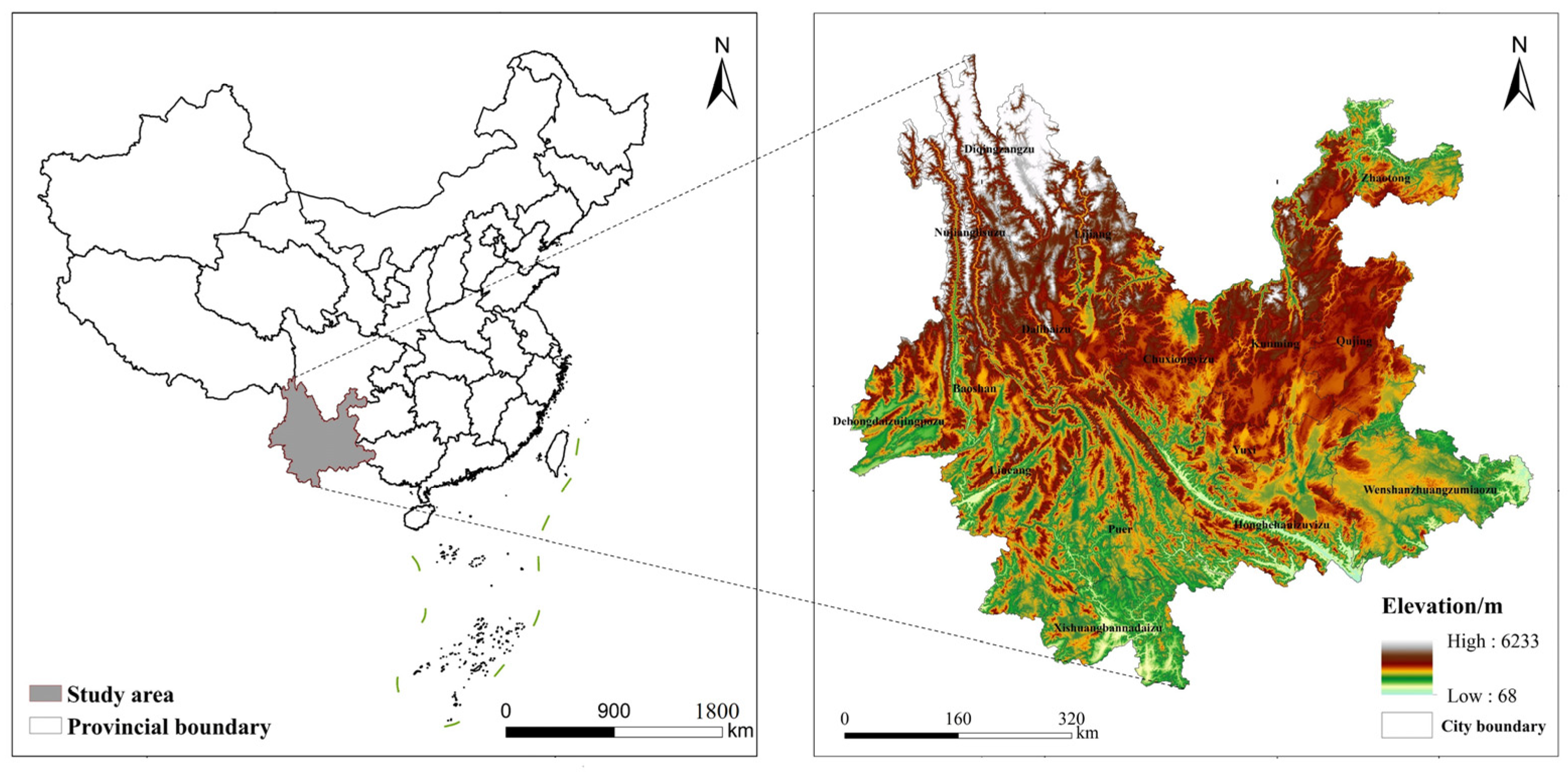
Yunnan Province is located in the southwestern part of China (Figure 1). The province features complex terrain, primarily consisting of plateau mountains, with numerous karst landforms and deep valleys. The elevation difference is 6663.6 m, with significant variations in altitude. The climate conditions in the study area are diverse, ranging from a temperate climate in the north to a subtropical climate in the south. Precipitation varies between 540 mm and 2300 mm. YNP is abundant in lakes and boasts a well-developed water system, offering ample water resources. The diverse climatic conditions and unique natural geographical features contribute to the province’s complex and diverse ecosystems, making it a crucial ecological barrier and a key area for water conservation. Economically, YNP’s main industries are agriculture and tourism. Over the past few years, as urbanization has rapidly increased, the province’s GDP has continued to grow, but it also faces challenges related to land use changes. Agricultural expansion and urban construction have strained land resources, resulting in the deterioration of some natural ecosystems. Many tourist attractions are close to ecologically important areas, and the development of tourism has led to more frequent land use changes in these areas [44]. In particular, around important water bodies like Dianchi Lake and Erhai Lake, pollution from urbanization and unreasonable development has led to ecological issues, including declining water quality and decreasing wetlands [45,46].
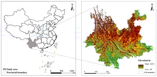
Figure 1.
Location of the YNP.
These issues pose a threat to the ESs and the stability of YNP’s environment, while also having negative impacts on the region’s sustainable development. YNP tries to implement ecological red line policy and basic farmland policy to protect forests, grassland and high-quality farmland to cope with land use change. Therefore, it is necessary to study the response of YNP regional ESV to land use change, and explore the future evolution trend of LULC and ESV under policy constraints, so as to provide advice for managers to optimize policies and help with sustainable development.
2.2. Data Sources and Processing
This study uses a variety of data, including LUCC data, topographic data, meteorological data, road network traffic data, NDVI, population data, GDP, and other multi-source datasets (Table 1). According to the research requirements, land use types for the years 2005, 2010, 2015, and 2020 were classified into six categories—farmland, forest land, grassland, water bodies, unused land, and built-up land. The spatial coordinates of the raster data were projected and transformed, and land use data were extracted based on the administrative boundaries of YNP. The data were rasterized and resampled to a resolution of 100 m × 100 m. To facilitate the ESVs calculation and visualization, we used the fishnet tool in ArcGIS to partition the study area into 4188 grids of 10 km × 10 km. Land use data for each grid were statistically analyzed, and the corresponding total ESVs for each grid were computed.

Table 1.
Data sources in this study.
3. Methodology
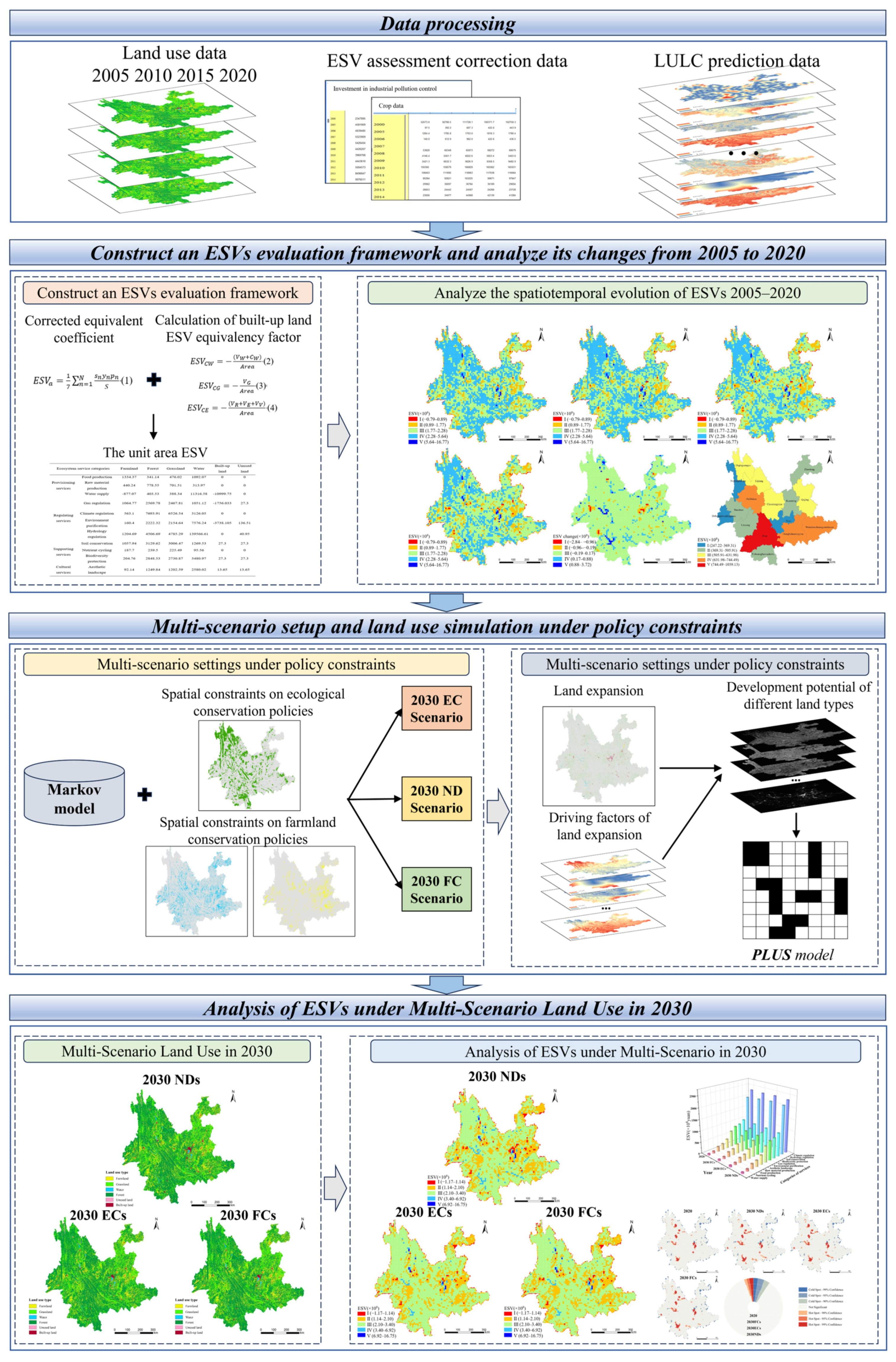
The workflow of this research is illustrated in Figure 2. Firstly, based on data cropping and coordinate transformation, the historical evolution characteristics of LULC in 2005, 2010, 2015 and 2020 are analyzed to extract land expansion patches, and the developmental potentials of various land types are calculated based on the selected influencing factors. Utilizing the spatial constraints of ecological conservation policy and farmland conservation policy to set up ECs and FCs, the Markov model is applied to calculate the land use demand prediction in 2030 under NDs, and is corrected again to get the demand prediction of ECs and FCs on the basis of the same. Following these steps, the PLUS model is utilized to obtain the LULC under different scenarios in 2030. Secondly, the ESVs equivalent unit table of YNP is constructed by correcting the existing ESVs equivalent coefficients and measuring the ESVs per unit of built-up land, considering the negative effects of built-up land. The spatiotemporal evolutions of ESVs from 2005 to 2020 and under different scenarios for 2030 are analyzed by combining the LULC data. Finally, the response characteristics of ESVs to LULC under different scenarios are analyzed, and suggestions are made regarding the future development of YNP.

Figure 2.
The framework diagram of this study (Note: ESVs—ecosystem service values, NDs—natural development scenarios, ECs—ecological conservation scenarios, FCs—farmland conservation scenarios).
3.1. Assessment of Ecosystem Service Values
The ESVs calculation method employs the unit coefficient method, which uses equivalent coefficients per unit area for computation. Using the ESVs assessment framework proposed by [4], Xie established the land ecosystem unit area ESVs assessment table for China and enhanced it in 2015 [47,48]. However, this coefficient was calculated at the national scale, and regional disparities result in variations in unit ESVs across provinces. Directly applying this coefficient to specific provinces introduces significant errors, so it must be adjusted according to local conditions. Based on previous research, this work calibrates the ESVs equivalent factors for YNP. The standard economic value of the unit factor for ESs is equivalent to 1/7 of the average market value of cereals per year. The formula is as follows:
where represents the planting area of the corresponding crop; denotes the yield level of the corresponding crop; is the market price of the corresponding crop; refers to the total planting area of all primary food crops; and represents the total number of categories for these key food crops.
In this study, the major food crops in YNP during the study period, namely, rice, maize, and wheat, are selected. The average price during the study period is used as the unit price for the crops, and the average unit yield of these three crops is used for calculation. This results in the base equivalent value coefficient for YNP of CNY 1334.37 per hectare.
Xie and most scholars consider the equivalent factor of built-up land to be zero [7,10,21,22]. However, in reality, the existence and development of built-up land depend on ecosystems, and they exert a detrimental influence on ESs through the generation of noise, the discharge of wastewater, exhaust gases, and solid waste [49]. This study employs the approach developed by Zhao to evaluate ESs provided by built-up land [23], including regulation, water supply, and environmental purification, and to assign specific values to the equivalent factors of built-up land. The specific formula is as follows:
is the water resource supply value per unit area of built-up land, is the cost of wastewater treatment for built-up land, is the water supply cost for built-up land, and represents the total area of built-up land.
is the gas regulation value per unit area of built-up land, and is the cost of exhaust gas treatment for built-up land.
represents the environmental purification value per unit area of built-up land. is the cost of residential waste treatment, is the cost of industrial waste treatment, and is the cost of noise pollution mitigation.
In conclusion, the unit area ESVs of YNP is shown in Table 2.
Table 2.
Ecosystem services value per unit area in YNP (unit: CNY/ha).
3.2. Spatiotemporal Analysis of Ecosystem Service Values
3.2.1. Spatial Autocorrelation
Global spatial autocorrelation is an effective method for describing the spatial distribution patterns of variables across an entire region [23]. The calculation formula is as follows:
where represents the total number of spatial units for ESVs evaluation, and represent the attribute values of the and spatial units, respectively, denotes the average ESVs, and represents the spatial weight value.
3.2.2. Hot Spot Analysis
Cold and hot spot analysis (Getis-Ord Gi*) is a widely utilized method for identifying the spatial distribution of cold and hot spot areas. It addresses the limitation of global spatial autocorrelation in determining the specific locations of clusters or dispersions, and accurately assesses the clustering degree of ESVs spatial distribution at high and low values [50]. The formula is as follows:
where represents the attribute value of feature , denotes the spatial weight between features and , and is the total number of features.
3.3. Future Land Use Multi-Scenario Simulation Based on the Markov-PLUS Model
3.3.1. Markov-PLUS Model
The PLUS model is a land use simulation model established within the framework of Cellular Automata (CA). It combines the Land Expansion Analysis Strategy (LEAS) with a CA model that utilizes multi-class random patch seeds (CARS) [39]. The LEAS module utilizes the random forest algorithm to explore the intrinsic relationships between land use expansion patterns and their driving factors, predicting the potential evolution probabilities of various land use types. Based on these predictions, the CA model simulates and forecasts future land use landscape patterns.
Compared to traditional land use simulation models, the PLUS model improves the accuracy of simulating land use/land cover (LULC) changes at the patch level by more effectively capturing nonlinear relationships [51]. It integrates various influencing factors, including topography, socio-economic conditions, and climate, to generate highly accurate and precise LULC spatial distribution results [39,52].
Overall, the PLUS model not only enhances the predictive accuracy of LULC modeling, but also contributes to offering deeper insights into the underlying mechanisms of ecosystems influenced by LULC changes, viewed through the lens of complex systems theory [53]. In this study, Patch-generating Land Use Simulation Model v1.4 was used for data processing and calculations.
3.3.2. Selection of Land Expansion Driving Factors
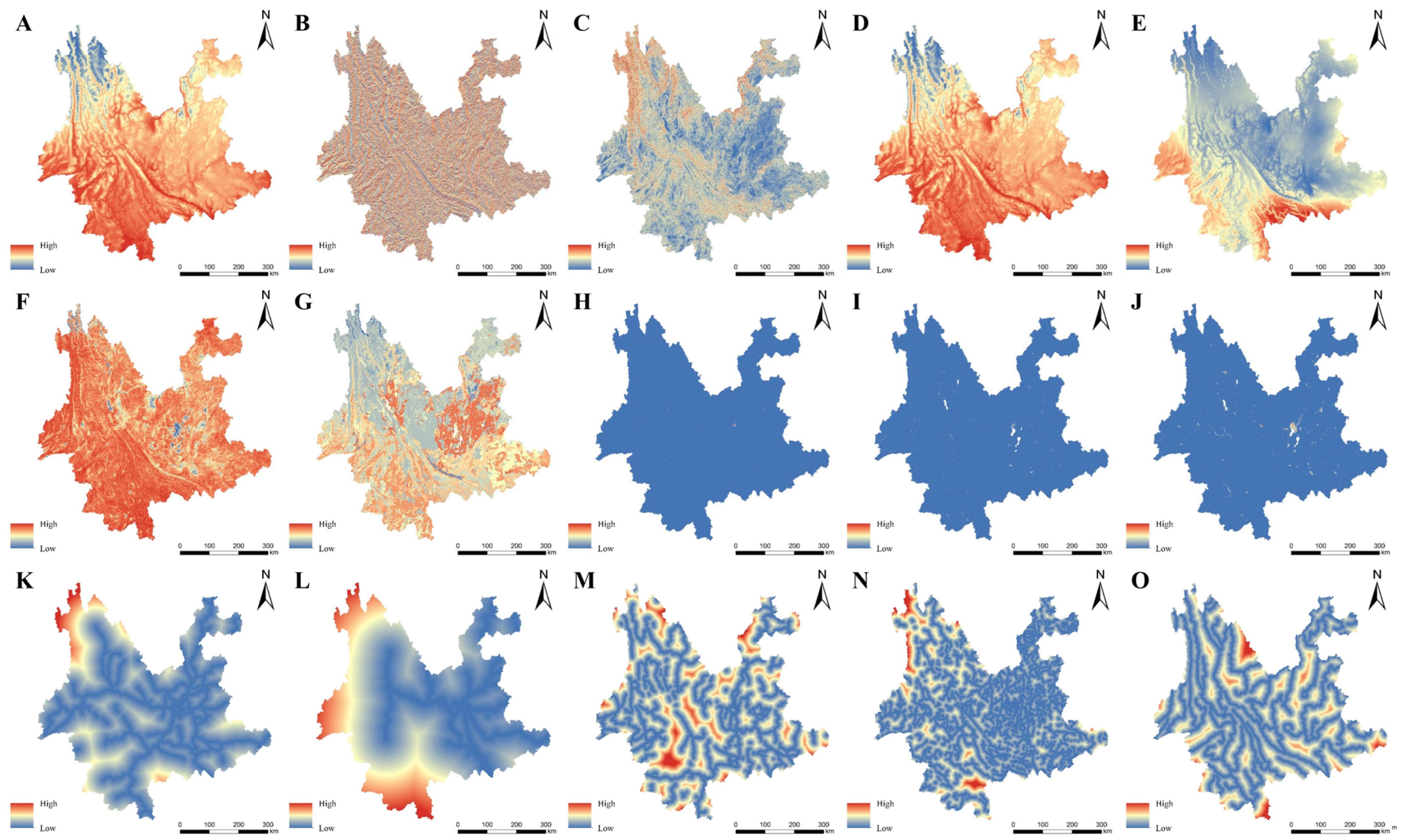
Land use patterns are directly or indirectly influenced by driving factors. Based on existing research experience, the characteristics of the YNP, data availability, and the quantifiability of driving factors, this study selects 15 driving factors for land use simulation, including elevation, slope, aspect, temperature, precipitation, normalized difference vegetation index (NDVI), distance to highways and railways, population density, and GDP density (Figure 3).
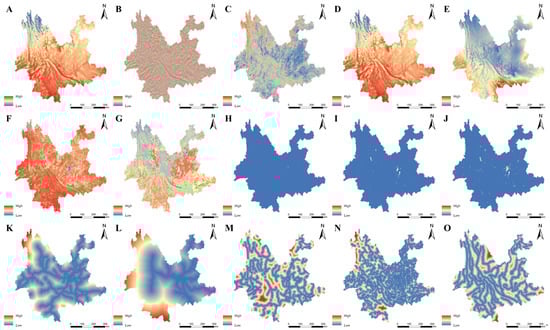
Figure 3.
Driving factors of land expansion. (A) DEM, (B) Aspect, (C) Slope, (D) Temperature, (E) Precipitation, (F) NDVI, (G) Soil type, (H) GDP, (I) Population, (J) Night light, (K) Distance to highway, (L) Distance to railway, (M) Distance to urban main roads, (N) Distance to urban secondary roads, (O) Distance to water.
3.3.3. Accuracy Verification
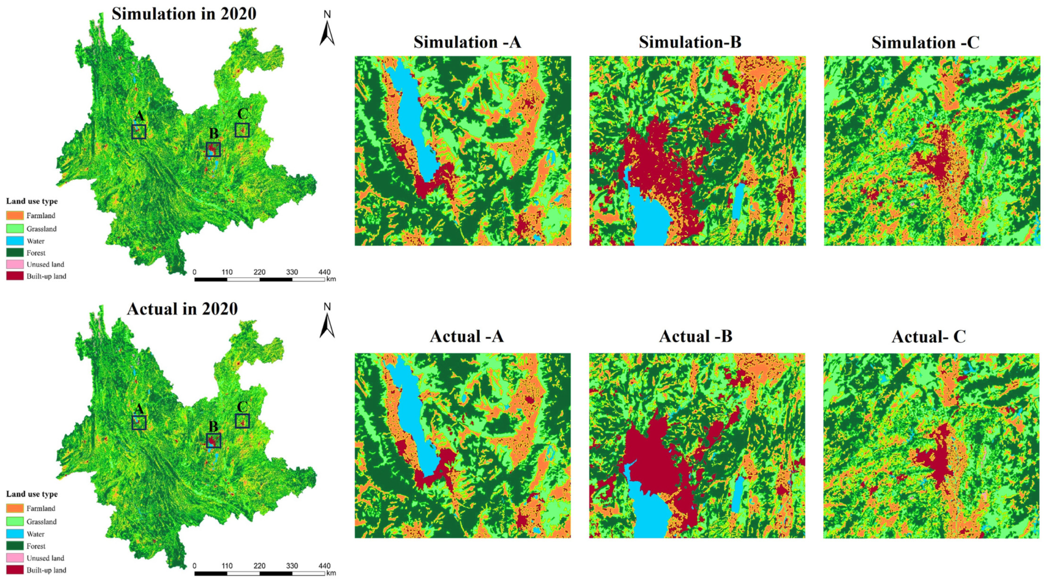
This study has utilized the 2010 land use data of YNP to simulate the 2020 land use data, which are subsequently compared with the real 2020 land use data to verify the model simulation’s correctness (Figure 4).

Figure 4.
Comparison of actual and modeled land use in 2020.
When evaluating the accuracy of the simulated data, the overall accuracy (OA) and the Kappa coefficient are here used as metrics to assess the overall precision of the simulated images. The formulas are as follows:
where represents the total number of grid cells, is the number of land use categories, indicates the number of correctly modeled grid cells for land use type , represents the total number of grid cells for this type in the simulation results, and represents the total number of grid cells for this type in the actual scenario. The OA index represents the likelihood that each random sample aligns with the actual LULC data, ranging from 0 to 1. Higher values, closer to 1, signify greater accuracy. A Kappa coefficient exceeding 0.75 signifies a strong agreement between observed and simulated results.
In this study, the PLUS model achieved a Kappa coefficient of 0.8914, surpassing the 0.75 threshold, along with an OA coefficient of 0.9022. These results strongly validate the PLUS model’s effectiveness and accuracy in forecasting future land use changes in YNP, making it a reliable tool for simulating land use dynamics in the province through 2030.
3.3.4. Multi-Scenario Settings Based on Policy Space Constraints
Scenario design is intended to help investigate potential pathways for future land use transition within YNP and to evaluate alterations in ESVs across various development trajectories, offering valuable insights for policymakers. Considering the current development status of YNP and its alignment with national land use planning and ecological protection strategies, three development scenarios were established. The specific rules for scenario setting are as follows:
- (1)
- Natural development scenario (NDs). Without considering human intervention or policy constraints, this scenario leverages historical land use data to model the region’s intrinsic development trajectory. No additional constraints are applied to the conversion processes, and the PLUS model is utilized to forecast land use patterns for 2030, forming the foundation for the analysis of the other two scenarios;
- (2)
- Ecological conservation scenarios (ECs). Through the implementation of the ecological red line policy, China has been enforcing the strict protection of key ecological function areas. In this scenario, for land within the ecological red line, the conversion of forest land, grassland and watershed land types will be strictly controlled, and for land outside the red line control area, the probability of conversion of other land types to forest land will be increased and the loss of forest land will be reduced, in order to meet the requirements for ecological conservation and maximize the ecological benefits of various land use types. Specific adjustments include decreasing the probability of forest land being converted into farmland, grassland, or built-up land by 80%, enhancing the probability of unused land transforming into farmland, grassland, or forest land by 30%, boosting the chance of farmland transitioning to forest land or grassland by 30% while lowering its conversion to built-up land by 30%, increasing the probability of grassland transitioning to forest land by 30% and reducing its shift to built-up land by 30%, and keeping all other conversion probabilities unchanged;
- (3)
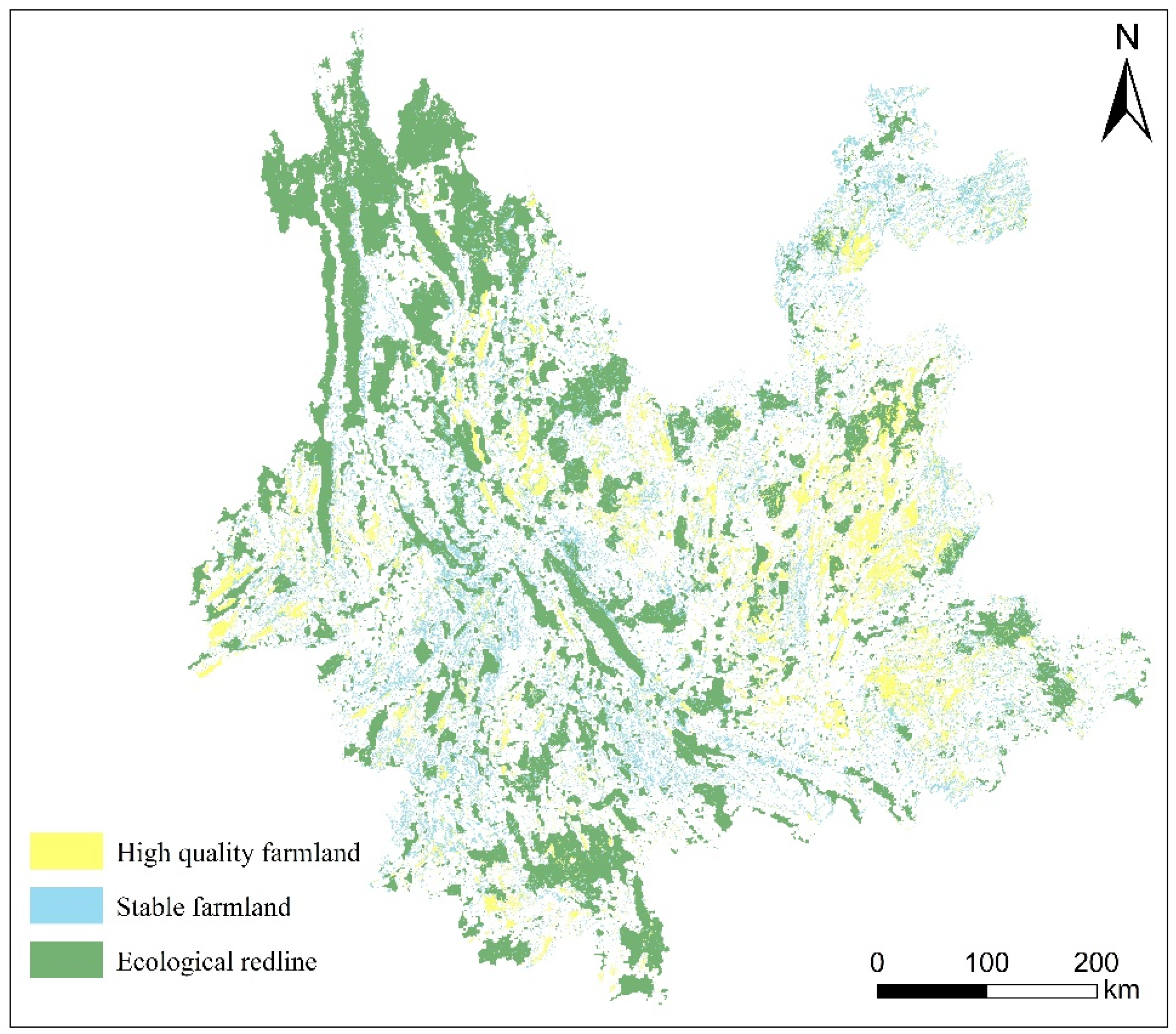
- Farmland conservation scenario (FCs). Farmland protection is closely tied to national food security. China’s permanent basic farmland policy ensures the strict preservation of high-quality farmland and stable farming areas, prohibiting their conversion to other land types. In this scenario, the farmland data for YNP from 2005, 2010, 2015, and 2020 are overlaid to identify consistently cultivated areas, representing stable farming lands, while areas with slopes less than 6° are identified as high-quality farmlands. These stable and high-quality farmland areas are designated as restricted zones for conversion (Figure 5). Additionally, the likelihood of conversion from farmland to built-up land outside the boundaries of the restricted area is reduced by 60%, the probability of transition from other land types is kept unchanged, and the conservation of farmland is strictly enforced.
 Figure 5. Restricted conversion areas in YNP.
4. Results
4.1. Spatiotemporal Analysis of Land Use/Land Cover Dynamics from 2005 to 2020
By analyzing the land use structure at four time points during the study period, it can be observed that forestland and grassland were the dominant land types in YNP (Supplementary Table S1). Together, these two categories consistently accounted for over 75% of the total area, reflecting the province’s abundant ecological resources. Among these, forestland occupied the largest proportion and showed a gradual upward trend during the study period, increasing from 219,026 km2 in 2005 to 220,011 km2 in 2020. Grassland exhibited a declining trend, decreasing from 88,885 km2 in 2005 to 86,066 km2 in 2020, a total reduction of 2819 km2. Its proportion dropped from 23.16% to 22.42%. Built-up land experienced the most notable expansion, with an increase of 2580 km2, reflecting the rapid pace of urbanization. Besides forestland and built-up land, the water area also grew by 1018 km2. Conversely, farmland and unused land showed overall reductions. Farmland decreased by 1196 km2, while unused land declined by 568 km2.
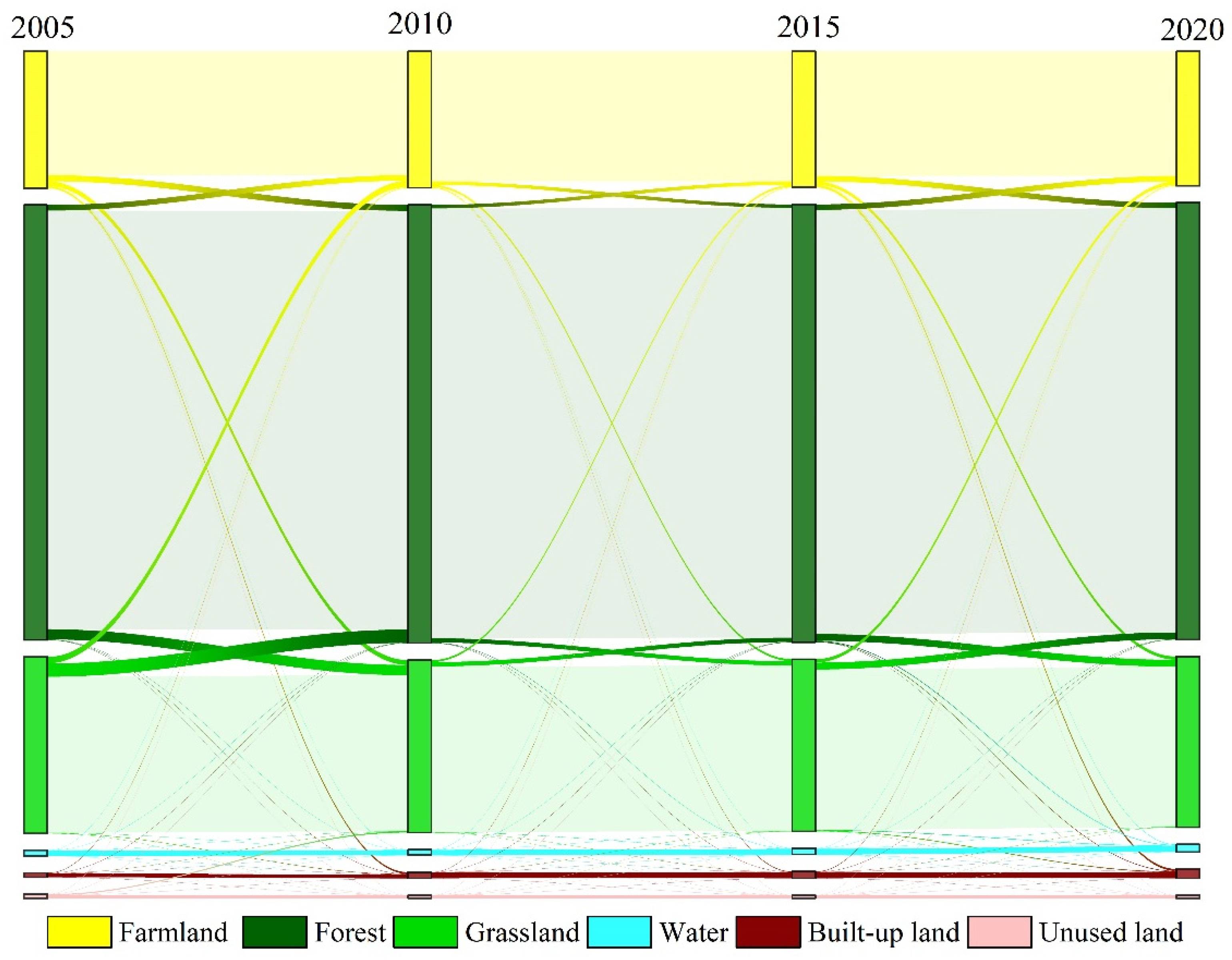
In terms of transition processes, the most prominent land use changes were grassland transitioning to forestland (8689.44 km2), forestland converting to grassland (7081.32 km2), and farmland transforming into forestland (4569.09 km2) (Figure 6). In addition to the mutual transitions among farmland, forestland, and grassland, notable changes also occurred from farmland and grassland to built-up land, with areas of 1829.43 km2 and 617.32 km2, respectively. From the perspective of final transition results, built-up land has emerged as the category with the largest inflow area.

Figure 6.
Land ese transfer Sankey map 2005–2020.
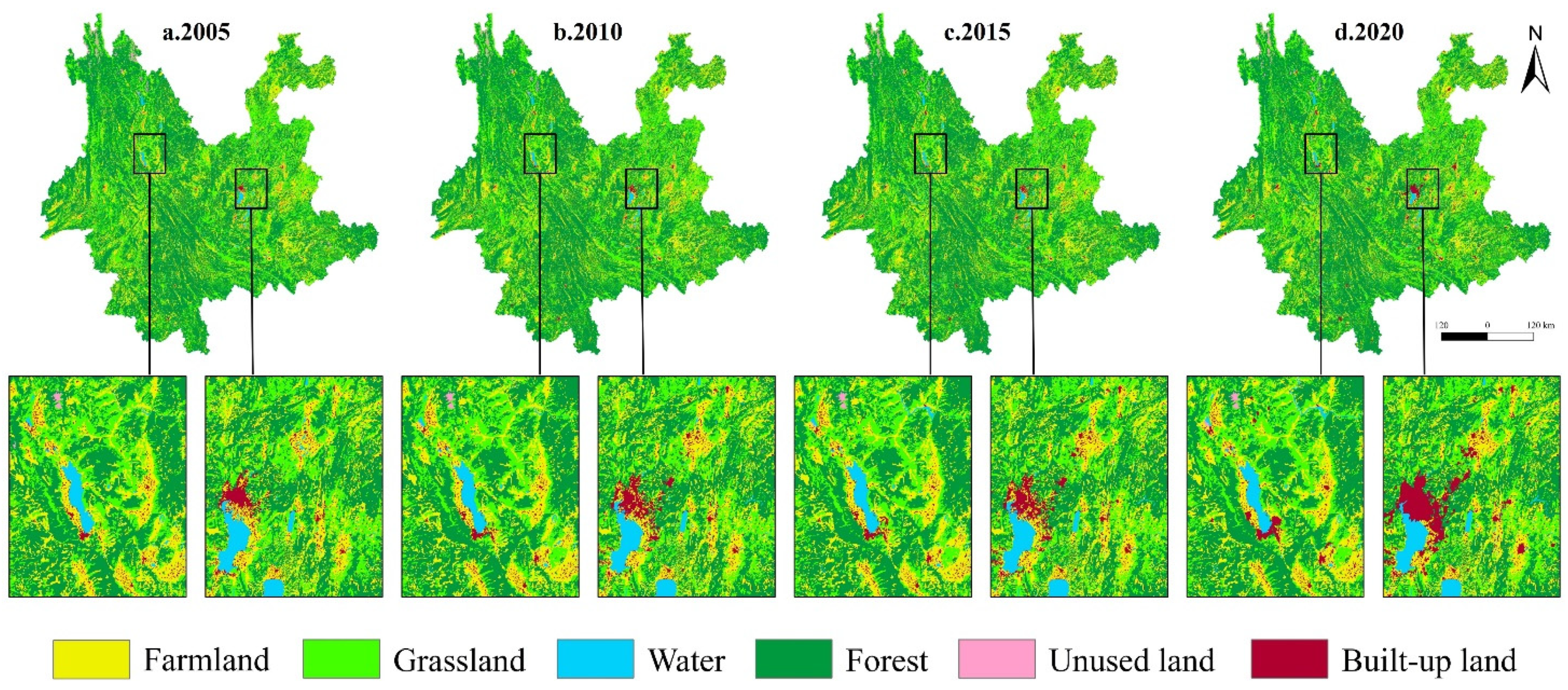
A deeper examination of the spatial distribution patterns of land use changes reveals significant spatial heterogeneity across YNP (Figure 7). The southwestern and northwestern parts of YNP contain a substantial portion of forestland resources. Farmland is predominantly located in the northeastern section, while built-up land is more densely clustered, primarily in the central–eastern region of YNP.

Figure 7.
Spatial patterns of land use in YNP between 2005 and 2020.
4.2. Analysis of Temporal and Spatial Evolution of Ecosystem Service Values in YNP (2005–2020)
Between 2005 and 2020, the total ESVs of YNP showed an initial decrease, subsequently followed by an increase. The ESVs for the four study points were CNY 870.426 billion, 869.491 billion, 873.009 billion, and 878.578 billion, respectively (Table 3). The ESVs in 2010 decreased slightly by CNY 0.935 billion compared to 2005, primarily due to the significant reduction in grassland ESVs, which led to the overall decline. However, from 2010 to 2020, ESVs consistently increased, resulting in a total growth of CNY 8.152 billion over the entire study period.
Table 3.
Changes of ESVs in YNP between 2005 to 2020 (unit: CNY billion).
Among the several land use types, water bodies experienced the largest increase in ESVs, with a growth of CNY 17.448 billion. This was followed by forestland, which remained the largest contributor to ESVs across all land use categories. Despite its limited area growth, forestland still accounted for a CNY 2.561 billion increase. On the other hand, the ESVs contributions from farmland, grassland, built-up land, and unused land all declined. Grassland experienced the largest decline, with its ESVs decreasing by CNY 6.954 billion, followed by built-up land, whose rapid expansion led to a reduction in ESVs by CNY 4.238 billion.
In YNP, the values of regulatory services and supporting services are relatively high, comprising an average of 66.39% and 22.94% of the total ESVs, respectively. Provisioning services and cultural services contribute 6.15% and 4.52% of the total ESVs, respectively. From the standpoint of ecosystem service categories, the ESVs of hydrological regulation and aesthetic landscape functions showed an increasing trend during the past 15 years. Conversely, the ESVs of other ecosystem service functions declined to differing extents.
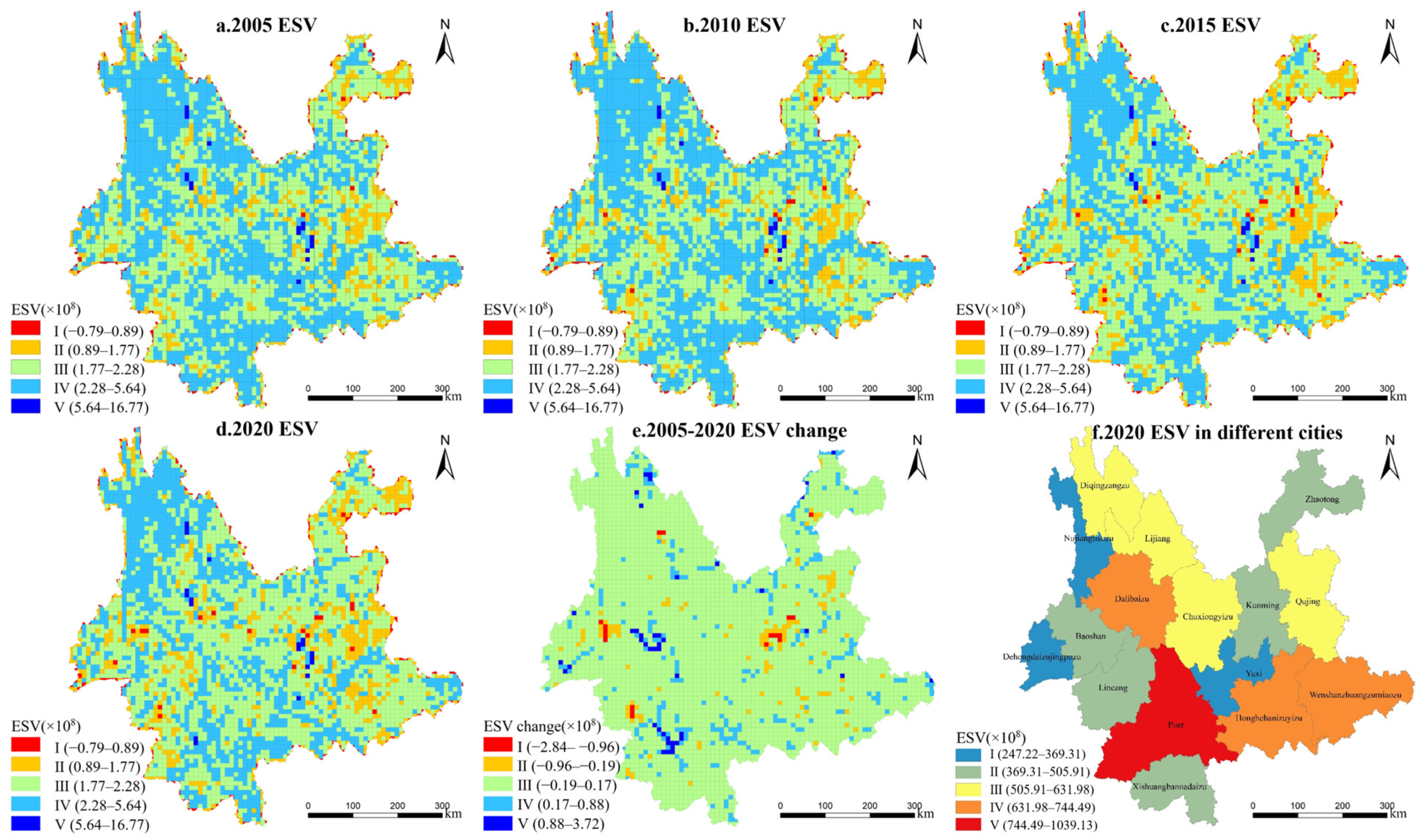
To further analyze the spatial patterns of ESV changes in YNP, the grid tool in ArcGIS has been used to create a mesh grid. The ESV intensity for each grid cell was calculated. Considering the study area’s size, topography, and terrain factors, a grid size of 10 km × 10 km was determined. The natural breaks method was utilized to categorize ESV intensities into five classifications, as follows: low-value regions, moderately low-value regions, medium-value regions, moderately high-value regions, and high-value regions. This has produced an ESVs intensity spatial distribution map (Figure 8). High-ESV areas are primarily located in the northwest and central regions, whereas low-ESV areas are predominantly distributed in the eastern and northeastern regions. Additionally, changes in ESV exhibit significant spatial and temporal heterogeneity. From 2005 to 2020, ESVs in the southeastern region remained stable. In contrast, the frequent land use changes in the southwestern and central areas due to urbanization led to significant spatial variations in ESVs. Areas with significant increases in ESVs were predominantly situated in the southwestern and southern areas. Conversely, substantial declines in ESVs were concentrated in the central areas. From an administrative perspective, the results show that Puer City has the highest total ESVs, while Dehong Dai and Jingpo Autonomous Prefecture have the lowest.

Figure 8.
Spatial and temporal variations in ESVs between 2005 and 2020.
4.3. Multi-Scenario Land Use Simulation
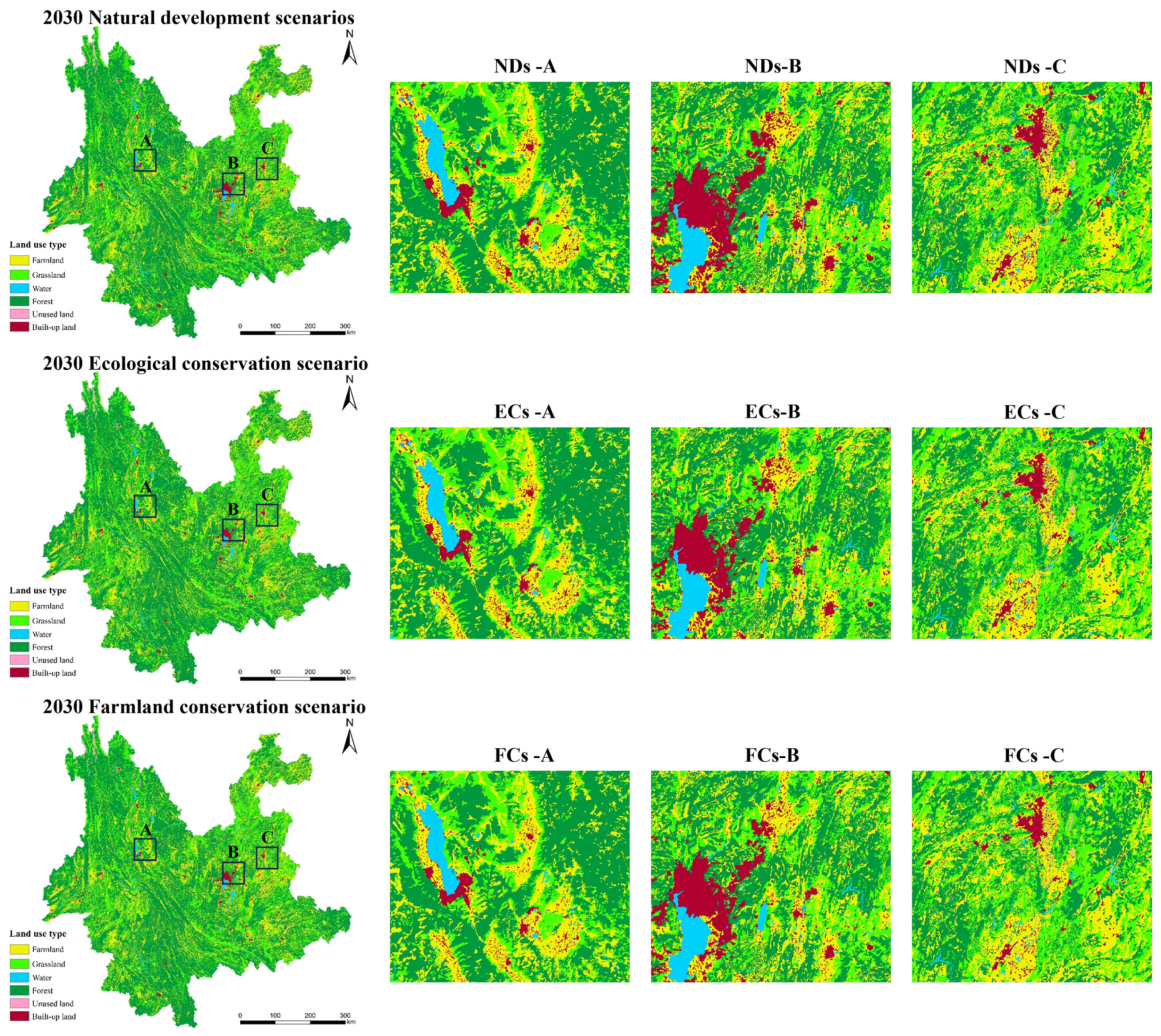
Using the PLUS model, the land use patterns in YNP for 2030 under three scenarios have been simulated, resulting in different spatial distributions (Figure 9). Forestland remains the most dominant land use type, widely distributed across the province, while farmland and grassland are primarily located in the lower-elevation areas of the eastern and western parts. Under NDs, the growth of built-up land occurs at a markedly quicker pace than in the other two scenarios, primarily at the expense of forestland and farmland surrounding existing urban areas. The spatial distribution patterns of land use under ECs and FCs are similar. The key difference lies in ECs, where the prioritization of forestland protection results in a greater presence of scattered forest patches near built-up areas. In contrast, the farmland protection scenario shows a lower degree of farmland fragmentation. The trend of urban expansion encroaching on farmland is more effectively curtailed, particularly in the eastern areas, where built-up land and farmland are centralized in low-lying areas. This difference is more pronounced in these flatter regions.

Figure 9.
Spatial and temporal patterns of ESVs dynamics from 2005 to 2020.
Further analysis of the quantitative characteristics of land use types under different scenarios reveals their respective area proportions (Supplementary Table S2). Compared with 2020, farmland area decreases under both NDs and ECs, by 844 km2 and 3102 km2, respectively. However, under FCs, farmland area shows an upward trend, increasing by 615 km2, consistent with the scenario’s prioritization of farmland conservation. Forestland area decreases under NDs and FCs by 718 km2 and 618 km2, respectively, while under ECs, forestland significantly expands, increasing by 4636 km2 while maintaining its original spatial pattern. Grassland area declines across all three scenarios, with ECs experiencing the largest decrease of 2739 km2, followed by decreases of 724 km2 and 706 km2 under NDs and FCs, respectively. In contrast, built-up land area increases under all three scenarios, albeit to varying extents. NDs continue the rapid urban expansion observed from 2005 to 2020, with their proportion rising from 1.24% in 2020 to 1.62% in 2030, an increase of 1463 km2. However, the expansion of built-up land is effectively curbed under ECs and FCs, with increases of 394 km2 and 270 km2, respectively. Notably, the growth of built-up land is smaller under FCs compared to the ECs.
The water area under FCs is 3829 km2, smaller than that under NDs (4658 km2) and ECs (4671 km2). The increase in farmland suppresses the trend of water area expansion. Unused land constitutes a minor portion of the total area, and exhibits no notable trend of change over time. However, compared with 2020, its area decreases across all three scenarios, indicating an increase in the development and utilization of unused land for urban purposes.
4.4. Ecosystem Service Value and Its Changes Under Simulated Scenarios
In YNP, the 2030 ESVs under NDs, ECs, and FCs are CNY 886.292 billion, 895.972 billion, and 883.805 billion, respectively. In comparison to 2020, NDs show an increase in ESVs of CNY 7.714 billion (Table 4). Among all land use types, water bodies exhibit the largest ESVs change, increasing by CNY 14.227 billion, while the ESVs for all other land use types decline. ECs demonstrate the most significant ESVs growth, with a rise of CNY 17.394 billion. Water bodies again contribute the largest growth, with an increase of CNY 14.437 billion, followed by forests, which add CNY 12.047 billion. Grasslands experience the largest decline, with a reduction in ESVs of CNY 6.756 billion. Under FCs, the ESVs see the smallest increase, at CNY 5.228 billion. However, this is the only scenario where the ESVs of farmland increase, showing an increase of CNY 0.334 billion. Additionally, this scenario records the smallest decrease in the ESVs of built-up land, with a drop of only CNY 0.443 billion.
Table 4.
ESVs under three simulated scenarios (unit: CNY billion).
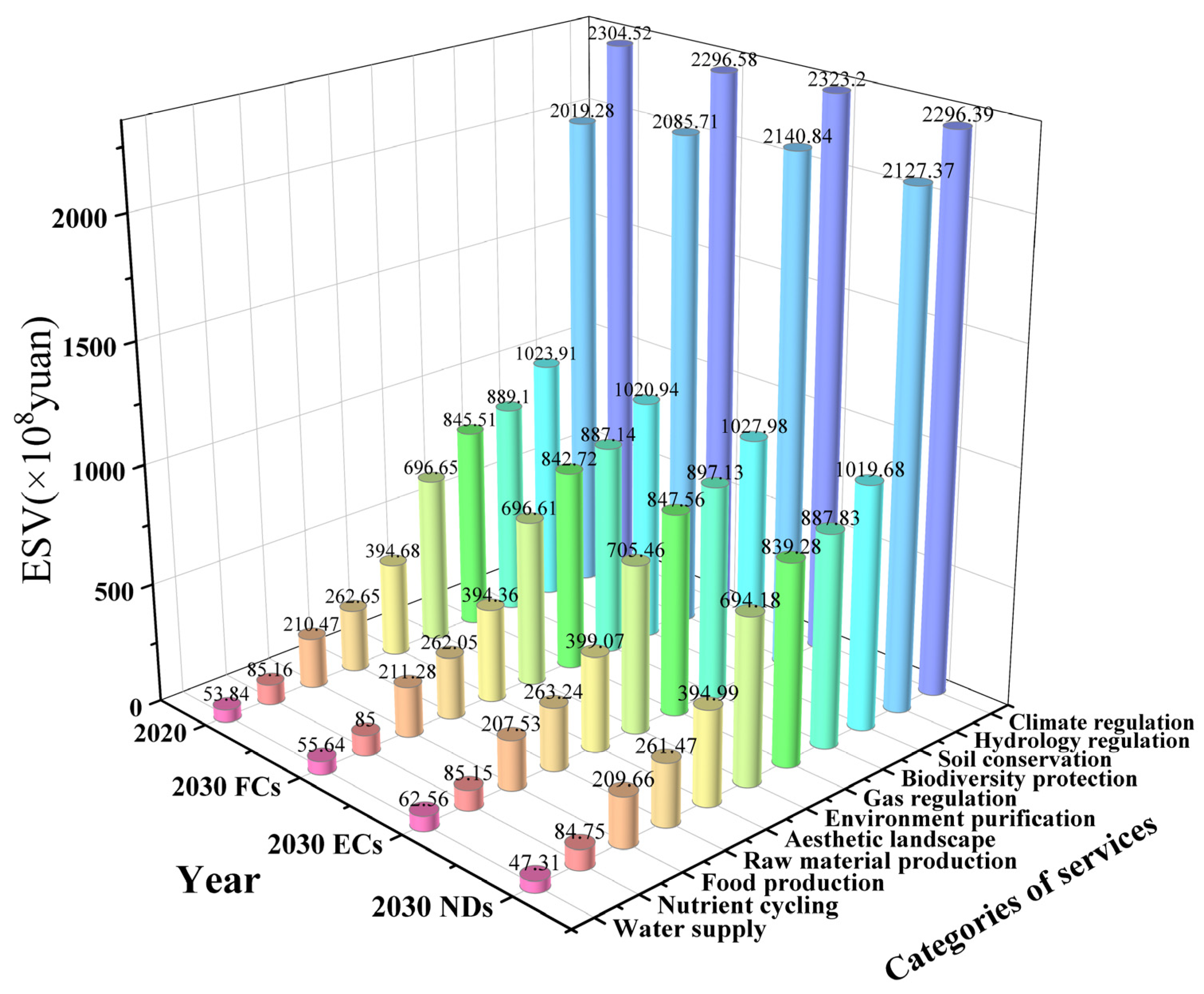
Under NDs in 2030, hydrological regulation and aesthetic landscape functions experienced increases of CNY 10.808 billion and 0.032 billion, respectively, while all other individual ESVs exhibited varying levels of decline compared to 2020 (Figure 10). In contrast, ECs exhibited entirely different trends. Only food production and water nutrient cycling functions decreased. All other functions showed increases, with notable changes in climate regulation and hydrological regulation functions, rising by CNY 1.868 billion and 12.156 billion, respectively. Under FCs, the ESVs for food production increased by CNY 0.082 billion, making this the only increase among the three scenarios. Other ESVs showed slight declines. Although the overall ESVs increased compared to 2020, the growth under this scenario was smaller than that in ECs and NDs.

Figure 10.
ESVs of different ecosystem service types under three scenarios.
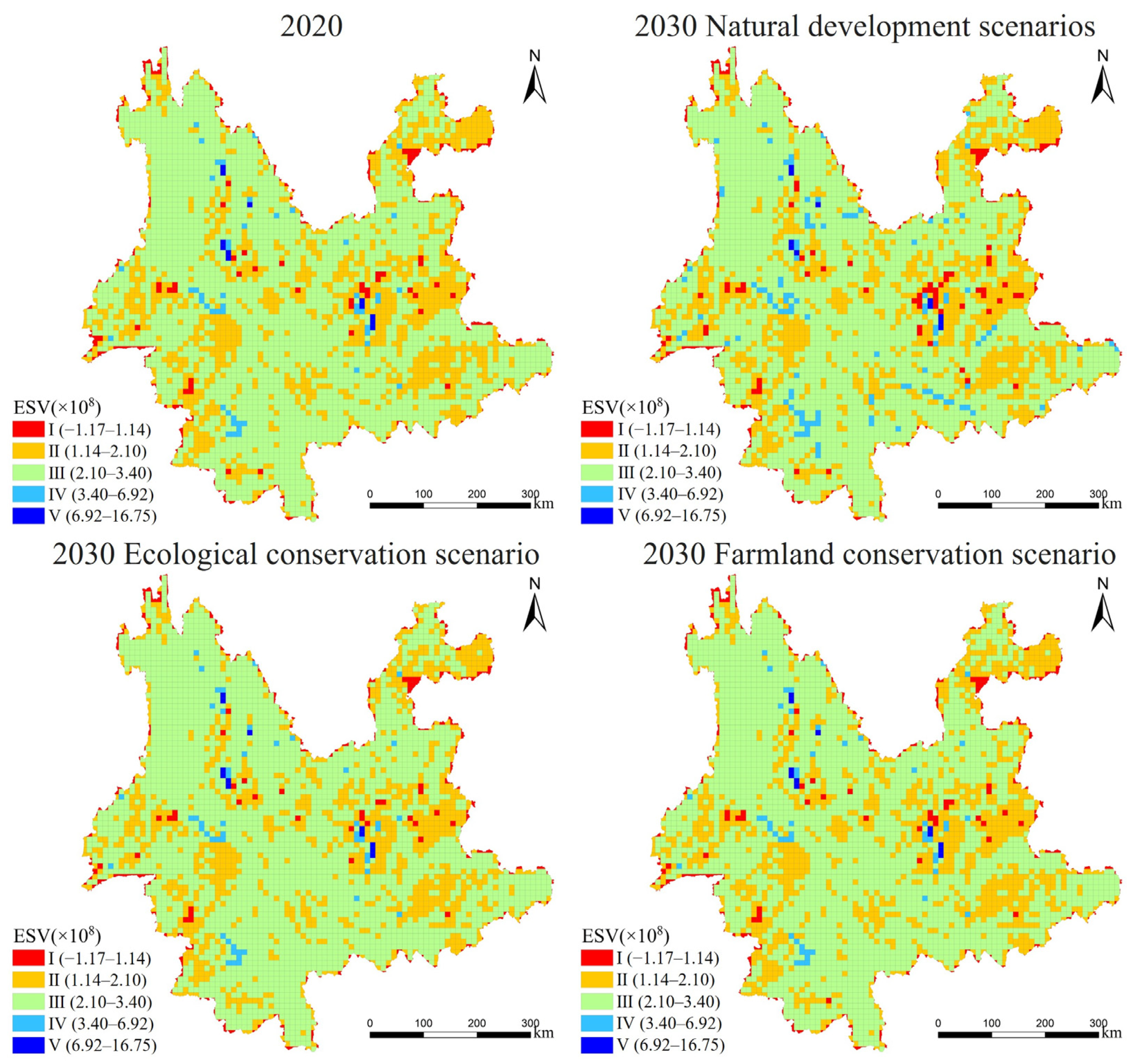
Spatially (Figure 11), compared to 2020, under NDs in 2030, the sub-high ESV regions in southern Puer City and Honghe Hani and Yi Autonomous Prefecture show a significant increase. Under ECs, the low-ESV regions in central Kunming City are noticeably smaller compared to NDs. In the western region, low-ESV areas shrink, and medium-value areas expand outward significantly. Although sub-high value areas in the south decrease slightly, the overall low-value areas are fewer, and ESVs see a clear overall increase. Under FCs, the spatial distribution of ESVs intensity is akin to that of ECs.

Figure 11.
ESV spatial distribution across various scenarios.
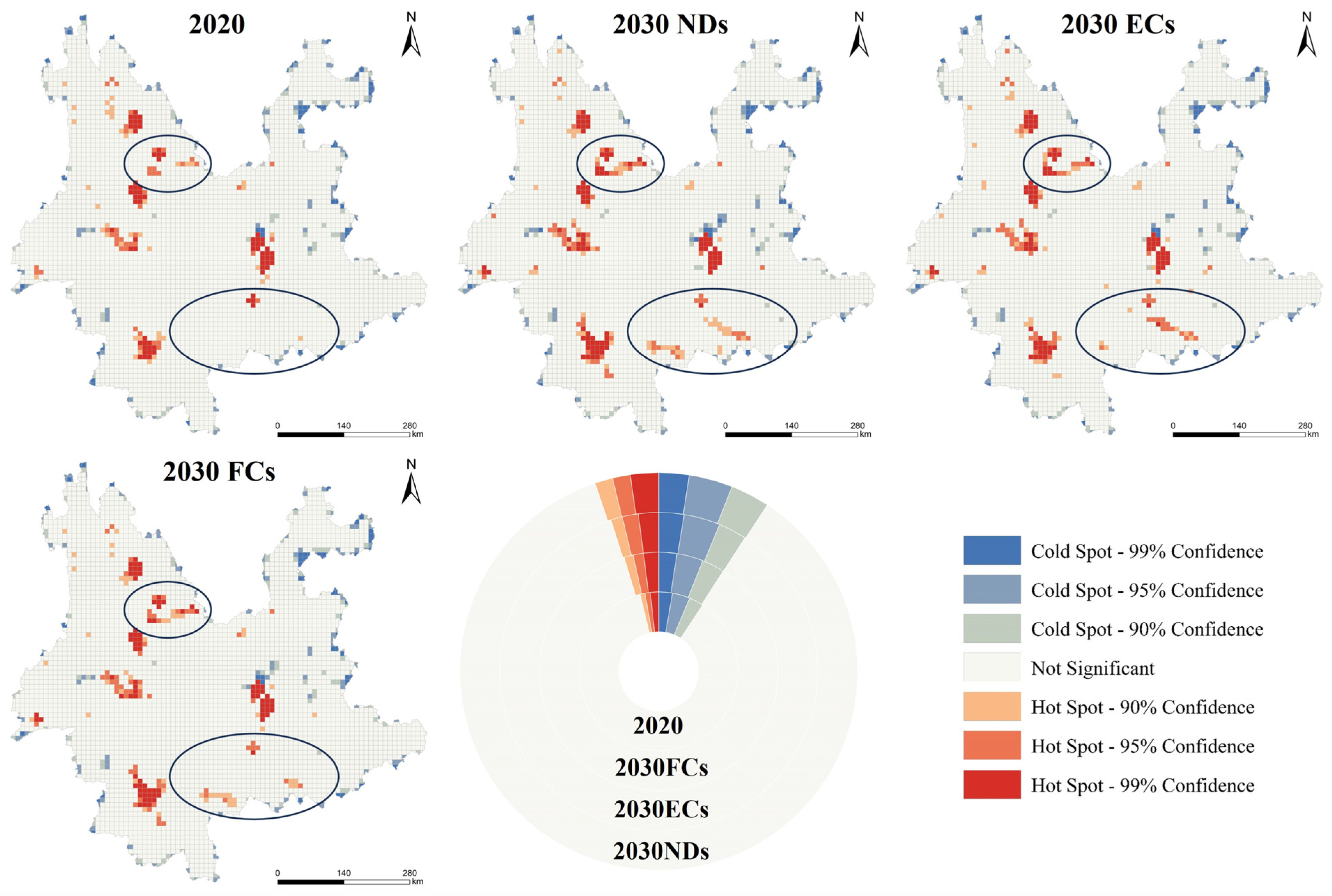
The analysis reveals that throughout the study period, Moran’s I index consistently hovered around 0.38, with Z-scores exceeding 30 and p-values below 0.001. These findings indicate a notable degree of clustering and strong spatial autocorrelation in the ESVs distribution. To further explore the spatial heterogeneity of ESVs changes across different scenarios, a hotspot analysis has bene performed using ESV values for each grid as spatial variables. As shown in Figure 12, hotspot areas in 2020 were mainly located in the northwest and central part, while cold spots were primarily located in areas with concentrated farmland along the study area boundaries. Compared to the spatial distributions of cold and hot spots in 2020, under all three scenarios in 2030, cold spot areas decreased, and the hotspot areas with 95% and 99% confidence intervals increased. Compared to NDs and ECs, FCs showed a reduction in hotspot areas in the southern region. This is mainly due to alterations in the spatial patterns of farmland and forest land.

Figure 12.
Spatial distribution of hot spot analysis.
5. Discussion
5.1. The Response of Ecosystem Service Values to Land Use Changes
Land use changes significantly influence the supply of ESs, thereby impacting ESVs [54,55]. Different land use transitions can exert both beneficial and adverse effects on ESVs [56]. In recent decades, rapid population growth, urbanization, and industrialization worldwide have led to the degradation or even disappearance of approximately 60% of ESs due to LULC changes. This negative trend is expected to continue throughout the first half of the 21st century [14,50]. However, through the active efforts of the Chinese government and the successful completion of various ecological restoration and conservation strategies, the Yunnan–Guizhou Plateau has achieved growth in forested areas and a significant increase in water bodies over the past two decades. This has partially alleviated the downward pressure on ESs caused by the expansion of built-up land and forest degradation [6].
This study, utilizing the ESVs coefficient adjusted by Xie [47], revealed that the total ESVs of YNP experienced an initial decline followed by a subsequent rise between 2005 and 2020, resulting in a net increase of CNY 8.152 billion. This finding is consistent with those from the research by Wang et al. on the Yunnan–Guizhou Plateau and global ESV trends [6,14]. Numerous studies indicate that an increase in farmland area can enhance certain ESs, such as food production, but it may also reduce others, particularly water supply and environmental purification [6,42,57,58]. In this study, the conversion of forestland and grassland to farmland had the most significant adverse effect on ESVs, resulting in losses of CNY 8.919 billion and 8.044 billion, respectively. Following this, the transformation of farmland and water bodies to built-up land caused losses of CNY 3.999 billion and 2.636 billion, respectively. These results are consistent with the existing understanding that urbanization-driven land use changes lead to substantial ESV reductions [29]. The most significant positive effect on ESVs came from the conversion of farmland to forestland, which contributed to an increase of CNY 9.390 billion. This transition can be attributed to the implementation of a series of ecological restoration projects in China, such as the Natural Forest Protection Program and the Grain for Green Program. These initiatives facilitated the reversion of farmland to grassland or forest, effectively mitigating ESV losses [59,60]. Water is essential for the provision of ESs [58], and water bodies have the highest unit-area ESVs among all land use types. YNP is rich in water resources, with six major river systems including the Jinsha, Nanpan, Yuan, Mekong, Salween, and Irrawaddy Rivers, as well as numerous lakes such as Dianchi and Erhai. Thanks to water resource management and conservation efforts, the water body area in YNP significantly increased by 36.20% from 2005 to 2020. The conversion of forestland and farmland to water bodies contributed to ESV increases of CNY 8.188 billion and 6.699 billion, respectively.
Moreover, it is noteworthy that ESVs exhibit significant spatial and temporal heterogeneity under the influence of LULC patterns. The ESVs hot spots are primarily located in the western and central regions of the YNP, which coincide with regions where water bodies and forestlands are concentrated. As the areas of these land use types increase, the hot spot regions tend to expand (Figure 12). Simultaneously, in areas with a high concentration of built-up land in the central region, ESV cold spot regions have shown a tendency to become more concentrated and enlarged over time. This indicates that the dynamic changes in YNP’s land use patterns, influenced by human activities, ecological restoration initiatives, and various natural environmental conditions, have substantially affected its ecosystem service values.
The mutual conversions among farmland, forestland, and built-up land are amongst the main drivers of the effects of land use changes on ESVs. Rapid urbanization has led to the conversion of extensive farmland into built-up land for urban and rural development, which is an irreversible LULC transition. The expansion of built-up land has had adverse effects on ESs. Meanwhile, the reduction in farmland has impacted food production services, posing a threat to food security. The Chinese government has implemented the “farmland balance policy” to ensure no net loss of farmland, with much of the newly added farmland coming from forestland. This has led to a conversion of forestland into farmland, contributing to a decrease in ESVs. However, a series of ecological restoration projects, such as the “Natural Forest Protection” and “Grain for Green” programs, have facilitated the transformation of low-quality farmland into forestland, thereby mitigating changes in ESVs. Additionally, the expansion of water areas and the improved connectivity of water systems have further enhanced the surrounding ecological environment [61,62], allowing ESs to be fully utilized and partially offsetting the ESVs losses caused by the expansion of built-up areas. Therefore, it is essential to focus on the impacts of rapid urbanization on ecosystems and recognize the irreversibility of farmland conversion into built-up land. Systematic land use optimization planning and measures should be implemented to balance reversible transitions among land use types. This approach can prevent human activities from further degrading ES functions and values, maintain ecological balance, and comprehensively promote the enhancement of ESVs.
5.2. Changes in Ecosystem Service Values Without Consideration of Built-Up Land
Since the start of the 21st century, the world has been experiencing unprecedented urbanization [63]. The rapid growth of built-up land has profoundly affected the structure and function of ecosystems at both regional and global scales [64]. Urban expansion and the proliferation of developed land have encroached on natural ecosystems, resulting in fragmentation, degradation, and a reduction in ESs [65]. Wu et al. demonstrated through multi-scale validation that changes in built-up land affect water-related ESs [66]. Similarly, Zhang et al. highlighted the gradient negative effects of built-up land on ESs during urbanization [8].
Currently, many scholars adopt the equivalent factor table proposed by Xie et al. to evaluate ESVs [47]. However, in this equivalent factor table, the ESVs of built-up land have not been independently calculated. Some researchers continue to use the ESVs per unit value for built-up land as set in this equivalent factor table, excluding it from ESVs calculations [7,10,21,22].
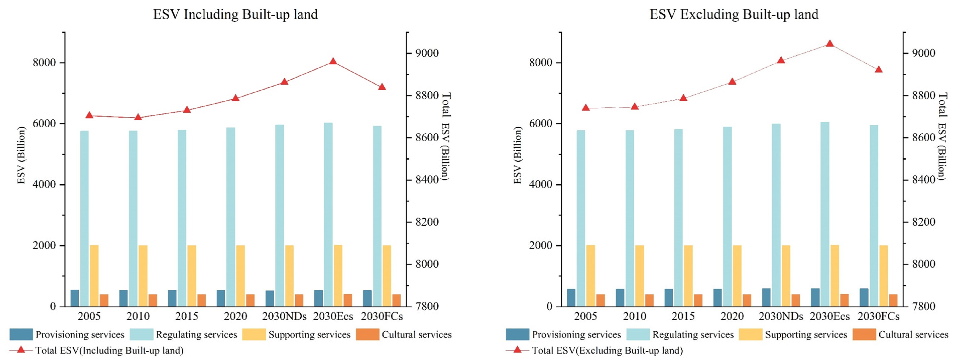
Shi et al. and Xing et al. considered the positive effects of artificial green spaces within built-up land on ESVs [67,68], while Zhao et al. analyzed the negative effects of built-up land on ESs from the perspectives of water resource supply, atmospheric conditions, and environmental purification [23]. Building on this foundation, this study incorporates the adverse effects of built-up land into the ESVs evaluation framework, and assesses and simulates past and future ESVs in YNP. By comparing the differences shown in Figure 13 between scenarios that include and exclude built-up land, we reveal distinct trends in ESV changes.

Figure 13.
Comparison of ESVs including and excluding built-up land.
From 2005 to 2020, when accounting for built-up land, the overall ESVs initially declined before increasing. It decreased to CNY 869.491 billion in 2010, and then increased to CNY 878.578 billion by 2020. From the perspectives of different service types, provisioning services and supporting services exhibited a gradual decline, while regulating services steadily increased, and cultural services showed a trend of first decreasing and then increasing. In contrast, excluding built-up land resulted in a steady increase in total ESVs from CNY 874.006 billion in 2005 to CNY 886.396 billion in 2020. Provisioning services, contrary to the case where built-up land is considered, increased annually to CNY 57.932 billion, while the trends for the other three service types remained consistent with those observed when built-up land was included.
For the 2030 simulation scenarios, the rankings of total ESVs were the same in both cases (with and without built-up land): ECs had the highest total ESVs, followed by NDs, with FCs having the lowest ESVs. In all three scenarios, the total ESVs excluding built-up land were higher than that including built-up land. When comparing individual service types, provisioning services showed a key difference—when accounting for built-up land, NDs had lower provisioning services than FCs, whereas the opposite was true without built-up land. This difference arises because, under the inclusion of built-up land, the negative effects of built-up land on water resource supply outweigh the impact of farmland on water resource supply.
In conclusion, land use changes, particularly changes in built-up land, significantly affect ESVs. Achieving sustainable development while maintaining high ecosystem service values requires balancing urbanization and ecological conservation.
5.3. Simulation of Different Scenarios Under Policy Spatial Constraints and Insights into the Future Development of YNP
Effective land use management is crucial for promoting sustainable development. Ecosystem service value assessment results can serve as an important reference for land use planning [41]. Rational decision-making, in turn, relies on accurate predictions of how different development scenarios impact ESVs. Previous studies have shown that the PLUS model outperforms other land use simulation models [16]. The PLUS model effectively simulates the spatial distribution of LULC in YNP by analyzing the driving variables of land expansion, and is widely applicable across different scales [39].
Based on a comprehensive analysis of natural geography, socioeconomic conditions, and accessibility, 15 key land use driving factors were selected. Considering YNP’s economic development and ecological protection needs, three simulation scenarios were carefully designed: NDs, ECs, and FCs. The study also incorporates spatial constraints from the ecological conservation red line and farmland conservation policies into the PLUS model, offering decision-makers insights into the potential effects of these policies on future land expansion.
Building on this, simulations of LULC distribution patterns in YNP under the three scenarios for 2030 have been conducted. The future trends in ESVs under these scenarios have been thoroughly analyzed, providing valuable insights for balancing urbanization, farmland protection, and ecological conservation in policymaking.
The results indicate that different land use policies (with varying land use conversion constraints) significantly impact the spatial distribution of land use, and have both beneficial and detrimental effects on ESVs. Under all three scenarios, total ESVs shows an increase compared to 2020, with overall improvements in ecological quality. This reflects the delayed effects of existing ecological measures, which continue to deliver benefits. In the ecological conservation scenario, forests are effectively preserved, and the quality of aquatic ecosystems significantly improves, with both forest and water body areas increasing. Under this scenario, YNP’s ESVs reach their maximum potential. However, the trend of declining farmland expands further compared to NDs, resulting in a significant decline in food production services. In the farmland conservation scenario, urban land expansion is restricted, halting the decline in farmland area and leading to its growth. Stable and high-quality farmland, particularly in flat areas near cities, is adequately protected. However, this limits urbanization-induced encroachment on farmland. At the same time, restrictions on certain farmland conversions suppress the expansion of water bodies, leading to a slight reduction in ESVs compared to NDs.
Overall, future land use policies are likely to have far-reaching impacts on regional ecosystem service functions, with protection policies for ecologically important areas significantly increasing total ESV while further restricting the supply of food production services, and protection policies for farmland limiting the growth rate of total ESV while increasing food production services. Balancing farmland protection, ecological conservation, and urbanization is essential. Decision-makers should carefully weigh the benefits and drawbacks to select land use development policies best suited to YNP, maximizing economic development, farmland protection, and ecological benefits.
5.4. Limitations and Future Prospects
This study has estimated the ESVs of YNP and predicted land use and ESVs under multiple scenarios. However, certain uncertainties and limitations remain.
Firstly, this study considers the adverse effects of built-up land on ecosystems and incorporates them into an improved equivalent coefficient table for ESVs. Nonetheless, given the intricate nature of human activities, a comprehensive assessment of their effects remains challenging. The study does not fully account for various elements included within built-up land, nor does it consider the positive contributions of built-up land to supporting services and cultural services. These aspects require further investigation in future research.
Secondly, spatial constraints such as stable high-quality farmland have been incorporated into the model’s scenario settings, identifying policy factors that could limit or guide land expansion. This provides valuable insights for future land use management. However, the spatial constraints are here not comprehensive enough. Future studies could enhance these constraints by integrating and adjusting them across scenarios to achieve win–win outcomes for different scenario objectives, and broaden the scope of application.
Thirdly, apart from land use changes, ESVs are shaped by several human factors (such as population distribution and socioeconomic policies) as well as natural elements (including topography, climate variations, and meteorological shifts). To better understand the mechanisms driving ESV changes and examine the synergies and trade-offs among various ESs, future studies should comprehensively integrate these human and natural factors.
6. Conclusions
In this study, the influence of built-up land has been accounted for by adjusting the ESVs coefficients, enabling the evaluation of ESVs in the YNP region from 2005 to 2020. Furthermore, spatial constraints from ecological conservation and farmland conservation policies were integrated into the scenario design. Three development scenarios for 2030 were established, and the PLUS model was utilized to predict the spatial distribution of LULC and ESVs in YNP under these scenarios with high accuracy. The findings indicate that forests, grasslands, and farmlands are the primary land use types in YNP. Between 2005 and 2020, while YNP experienced rapid urbanization, it also showed improving ESs. Against the backdrop of a number of ecological restoration methods, the ecological degradation caused by economic development was mitigated. The total ESVs exhibited an initial decline followed by a subsequent increase, rising from CNY 8704.26 billion to 8785.78 billion, representing a growth rate of 0.94%. Changes in the LULC patterns significantly impacted ESVs. Forest restoration and increased water area positively influenced regulating services, leading to significant growth. However, the expansion of built-up land and the reduction in farmland caused slight declines in provisioning services and supporting services. While the total ESVs increased, the risk of local ESV declines also rose. Simulating YNP’s ESVs in 2030 under different scenarios has revealed that continuing forest protection measures could maximize the total ESVs, but this would further reduce farmland area. The strict protection of stable, high-quality farmland slows the expansion of built-up land and ensures food production, but it also somewhat hinders the expansion of water areas, slowing the growth of total ESVs. Therefore, we suggest that when advancing ecological restoration efforts, equal attention should be given to protecting high-quality farmland. Balancing ecological conservation, farmland protection, and urbanization is essential to achieving regional coordinated and sustainable development. By predicting and comparing the distribution pattern of LULCs and the development trend of ESVs under different scenarios, and analyzing the possible impacts of existing policy constraints on LULCs and ESVs, the study can provide references to improve ESVs and optimize the pattern of LULCs, and can help managers to adjust policies in a targeted manner. In the future, further research can be conducted on factors other than land use change to better understand the mechanisms driving changes in ESV, and to test the synergies and trade-offs between various ESs for coordinated and sustainable regional development.
Supplementary Materials
The following supporting information can be downloaded at: https://www.mdpi.com/article/10.3390/land14030601/s1.
Author Contributions
Conceptualization, C.Z.; methodology, C.Z.; software, C.Z. and H.D.; validation, Z.W. and H.L.; formal analysis, C.Z.; investigation, C.Z. and H.L.; resources, Z.W.; data curation, C.Z.; writing—original draft preparation, C.Z.; writing—review and editing, C.Z., Z.W. and H.L.; visualization, C.Z.; supervision, Z.W.; project administration, C.Z., H.D. and H.L.; funding acquisition, Z.W. All authors have read and agreed to the published version of the manuscript.
Funding
This research was funded by the Key Project from the National Social Science Foundation of China, grant number 23AZD058.
Data Availability Statement
The original contributions presented in the study are included in the article; further inquiries can be directed to the corresponding author.
Conflicts of Interest
The authors declare no conflicts of interest.
References
- Qiu, H.; Hu, B.; Zhang, Z. Impacts of Land Use Change on Ecosystem Service Value Based on SDGs Report—Taking Guangxi as an Example. Ecol. Indic. 2021, 133, 108366. [Google Scholar] [CrossRef]
- Guan, Y.; Qiang, Y.; Qu, Y.; Lu, W.; Xiao, Y.; Chu, C.; Xiong, S.; Shao, C. Environmental Sustainability and Beautiful China: A Study of Indicator Identification and Provincial Evaluation. Environ. Impact Assess. Rev. 2024, 105, 107452. [Google Scholar] [CrossRef]
- Zhang, X.; Ren, W.; Peng, H. Urban Land Use Change Simulation and Spatial Responses of Ecosystem Service Value Under Multiple Scenarios: A Case Study of Wuhan, China. Ecol. Indic. 2022, 144, 109526. [Google Scholar] [CrossRef]
- Costanza, R.; d’Arge, R.; de Groot, R.; Farber, S.; Grasso, M.; Hannon, B.; Limburg, K.; Naeem, S.; ONeill, R.V.; Paruelo, J.; et al. The Value of the World’s Ecosystem Services and Natural Capital. Nature 1997, 387, 253–260. [Google Scholar] [CrossRef]
- Kulaixi, Z.; Chen, Y.; Wang, C.; Xia, Q. Spatial Differentiation of Ecosystem Service Value in an Arid Region: A Case Study of the Tarim River Basin, Xinjiang. Ecol. Indic. 2023, 151, 110249. [Google Scholar] [CrossRef]
- Wang, Z.-J.; Liu, S.-J.; Li, J.-H.; Pan, C.; Wu, J.-L.; Ran, J.; Su, Y. Remarkable Improvement of Ecosystem Service Values Promoted by Land Use/Land Cover Changes on the Yungui Plateau of China during 2001–2020. Ecol. Indic. 2022, 142, 109303. [Google Scholar] [CrossRef]
- Jing, X.; Tian, G.; He, Y.; Wang, M. Spatial and Temporal Differentiation and Coupling Analysis of Land Use Change and Ecosystem Service Value in Jiangsu Province. Ecol. Indic. 2024, 163, 112076. [Google Scholar] [CrossRef]
- Zhang, X.-L.; Niu, C.-H.; Ma, S.; Wang, L.-J.; Hu, H.-B.; Jiang, J. Exploring Ecological Compensation Standards in the Urbanization Process: An Ecosystem Service Value-Based Perspective. Ecol. Indic. 2024, 166, 112510. [Google Scholar] [CrossRef]
- Gu, Y.; Lin, N.; Cao, B.; Ye, X.; Pang, B.; Du, W.; Dou, H.; Zou, C.; Xu, C.; Xu, D.; et al. Assessing the Effectiveness of Ecological Conservation Red Line for Mitigating Anthropogenic Habitat Degradation in River Corridors. Ecol. Indic. 2023, 154, 110742. [Google Scholar] [CrossRef]
- Wen, X.; Wang, J.; Han, X. Impact of Land Use Evolution on the Value of Ecosystem Services in the Returned Farmland Area of the Loess Plateau in Northern Shaanxi. Ecol. Indic. 2024, 163, 112119. [Google Scholar] [CrossRef]
- Wu, Y.; Shan, L.; Guo, Z.; Peng, Y. Cultivated Land Protection Policies in China Facing 2030: Dynamic Balance System versus Basic Farmland Zoning. Habitat Int. 2017, 69, 126–138. [Google Scholar] [CrossRef]
- Goldstein, J.H.; Caldarone, G.; Duarte, T.K.; Ennaanay, D.; Hannahs, N.; Mendoza, G.; Polasky, S.; Wolny, S.; Daily, G.C. Integrating Ecosystem-Service Tradeoffs into Land-Use Decisions. Proc. Natl. Acad. Sci. USA 2012, 109, 7565–7570. [Google Scholar] [CrossRef]
- Staiano, L.; Camba Sans, G.H.; Baldassini, P.; Gallego, F.; Texeira, M.A.; Paruelo, J.M. Putting the Ecosystem Services Idea at Work: Applications on Impact Assessment and Territorial Planning. Environ. Dev. 2021, 38, 100570. [Google Scholar] [CrossRef]
- Costanza, R.; de Groot, R.; Sutton, P.; van der Ploeg, S.; Anderson, S.J.; Kubiszewski, I.; Farber, S.; Turner, R.K. Changes in the Global Value of Ecosystem Services. Glob. Environ. Change 2014, 26, 152–158. [Google Scholar] [CrossRef]
- Na, L.; Zhao, Y.; Feng, C.-C.; Guo, L. Regional Ecological Risk Assessment Based on Multi-Scenario Simulation of Land Use Changes and Ecosystem Service Values in Inner Mongolia, China. Ecol. Indic. 2023, 155, 111013. [Google Scholar] [CrossRef]
- Luan, C.; Liu, R.; Li, Y.; Zhang, Q. Comparison of Various Models for Multi-Scenario Simulation of Land Use/Land Cover to Predict Ecosystem Service Value: A Case Study of Harbin-Changchun Urban Agglomeration, China. J. Clean. Prod. 2024, 478, 144012. [Google Scholar] [CrossRef]
- Jiang, Y.; Du, G.; Teng, H.; Wang, J.; Li, H. Multi-Scenario Land Use Change Simulation and Spatial Response of Ecosystem Service Value in Black Soil Region of Northeast China. Land 2023, 12, 962. [Google Scholar] [CrossRef]
- Tolessa, T.; Senbeta, F.; Kidane, M. The Impact of Land Use/Land Cover Change on Ecosystem Services in the Central Highlands of Ethiopia. Ecosyst. Serv. 2017, 23, 47–54. [Google Scholar] [CrossRef]
- Rahman, M.M.; Szabó, G. Impact of Land Use and Land Cover Changes on Urban Ecosystem Service Value in Dhaka, Bangladesh. Land 2021, 10, 793. [Google Scholar] [CrossRef]
- Xie, G.; Lu, C.-X.; Leng, Y.-F.; Zheng, D.U.; Li, S. Ecological Assets Valuation of the Tibetan Plateau. J. Nat. Resour. 2003, 18, 189–196. [Google Scholar]
- Wei, R.; Fan, Y.; Wu, H.; Zheng, K.; Fan, J.; Liu, Z.; Xuan, J.; Zhou, J. The Value of Ecosystem Services in Arid and Semi-Arid Regions: A Multi-Scenario Analysis of Land Use Simulation in the Kashgar Region of Xinjiang. Ecol. Model. 2024, 488, 110579. [Google Scholar] [CrossRef]
- Xiao, J.; Zhang, Y.; Xu, H. Response of Ecosystem Service Values to Land Use Change, 2002–2021. Ecol. Indic. 2024, 160, 111947. [Google Scholar] [CrossRef]
- Zhao, Y.; Zhang, X.; Wu, Q.; Huang, J.; Ling, F.; Wang, L. Characteristics of Spatial and Temporal Changes in Ecosystem Service Value and Threshold Effect in Henan Along the Yellow River, China. Ecol. Indic. 2024, 166, 112531. [Google Scholar] [CrossRef]
- Song, W.; Deng, X. Land-Use/Land-Cover Change and Ecosystem Service Provision in China. Sci. Total Environ. 2017, 576, 705–719. [Google Scholar] [CrossRef]
- Abbasnezhad, B.; Abrams, J.B.; Wenger, S.J. The Impact of Projected Land Use Changes on the Availability of Ecosystem Services in the Upper Flint River Watershed, USA. Land 2024, 13, 893. [Google Scholar] [CrossRef]
- Anley, M.A.; Minale, A.S.; Haregeweyn, N.; Gashaw, T. Assessing the Impacts of Land Use/Cover Changes on Ecosystem Service Values in Rib Watershed, Upper Blue Nile Basin, Ethiopia. Trees For. People 2022, 7, 100212. [Google Scholar] [CrossRef]
- El-Hamid, H.T.A.; Nour-Eldin, H.; Rebouh, N.Y.; El-Zeiny, A.M. Past and Future Changes of Land Use/Land Cover and the Potential Impact on Ecosystem Services Value of Damietta Governorate, Egypt. Land 2022, 11, 2169. [Google Scholar] [CrossRef]
- Kindu, M.; Schneider, T.; Teketay, D.; Knoke, T. Changes of Ecosystem Service Values in Response to Land Use/Land Cover Dynamics in Munessa-Shashemene Landscape of the Ethiopian Highlands. Sci. Total Environ. 2016, 547, 137–147. [Google Scholar] [CrossRef]
- Hasan, S.S.; Zhen, L.; Miah, M.G.; Ahamed, T.; Samie, A. Impact of Land Use Change on Ecosystem Services: A Review. Environ. Dev. 2020, 34, 100527. [Google Scholar] [CrossRef]
- Chen, W.; Zhang, X.; Huang, Y. Spatial and Temporal Changes in Ecosystem Service Values in Karst Areas in Southwestern China Based on Land Use Changes. Environ. Sci. Pollut. Res. 2021, 28, 45724–45738. [Google Scholar] [CrossRef]
- Liu, X.; Li, Y.; Lu, J.; Song, T.; Zhang, S. Urban Growth Simulation Guided by Ecosystem Service Trade-Offs in Wuhan Metropolitan Area: Methods and Implications for Spatial Planning. Ecol. Indic. 2024, 167, 112687. [Google Scholar] [CrossRef]
- Li, Q.; Wang, L.; Gul, H.N.; Li, D. Simulation and Optimization of Land Use Pattern to Embed Ecological Suitability in an Oasis Region: A Case Study of Ganzhou District, Gansu Province, China. J. Environ. Manag. 2021, 287, 112321. [Google Scholar] [CrossRef] [PubMed]
- Beroho, M.; Briak, H.; Cherif, E.K.; Boulahfa, I.; Ouallali, A.; Mrabet, R.; Kebede, F.; Bernardino, A.; Aboumaria, K. Future Scenarios of Land Use/Land Cover (LULC) Based on a CA-Markov Simulation Model: Case of a Mediterranean Watershed in Morocco. Remote Sens. 2023, 15, 1162. [Google Scholar] [CrossRef]
- Mansour, S.; Al-Belushi, M.; Al-Awadhi, T. Monitoring Land Use and Land Cover Changes in the Mountainous Cities of Oman Using GIS and CA-Markov Modelling Techniques. Land Use Policy 2020, 91, 104414. [Google Scholar] [CrossRef]
- Li, L.; Huang, X.; Yang, H. Scenario-Based Urban Growth Simulation by Incorporating Ecological-Agricultural-Urban Suitability into a Future Land Use Simulation Model. Cities 2023, 137, 104334. [Google Scholar] [CrossRef]
- Lin, J.; He, P.; Yang, L.; He, X.; Lu, S.; Liu, D. Predicting Future Urban Waterlogging-Prone Areas by Coupling the Maximum Entropy and FLUS Model. Sustain. Cities Soc. 2022, 80, 103812. [Google Scholar] [CrossRef]
- Ma, S.; Huang, J.; Wang, X.; Fu, Y. Multi-Scenario Simulation of Low-Carbon Land Use Based on the SD-FLUS Model in Changsha, China. Land Use Policy 2025, 148, 107418. [Google Scholar] [CrossRef]
- Huang, C.; Zhou, Y.; Wu, T.; Zhang, M.; Qiu, Y. A Cellular Automata Model Coupled with Partitioning CNN-LSTM and PLUS Models for Urban Land Change Simulation. J. Environ. Manag. 2024, 351, 119828. [Google Scholar] [CrossRef]
- Liang, X.; Guan, Q.; Clarke, K.C.; Liu, S.; Wang, B.; Yao, Y. Understanding the Drivers of Sustainable Land Expansion Using a Patch-Generating Land Use Simulation (PLUS) Model: A Case Study in Wuhan, China. Comput. Environ. Urban Syst. 2021, 85, 101569. [Google Scholar] [CrossRef]
- Liu, Y.; Jing, Y.; Han, S. Multi-Scenario Simulation of Land Use/Land Cover Change and Water Yield Evaluation Coupled with the GMOP-PLUS-InVEST Model: A Case Study of the Nansi Lake Basin in China. Ecol. Indic. 2023, 155, 110926. [Google Scholar] [CrossRef]
- Luan, C.; Liu, R.; Zhang, Q.; Sun, J.; Liu, J. Multi-Objective Land Use Optimization Based on Integrated NSGA–II–PLUS Model: Comprehensive Consideration of Economic Development and Ecosystem Services Value Enhancement. J. Clean. Prod. 2024, 434, 140306. [Google Scholar] [CrossRef]
- Wu, C.; Wang, Z. Multi-Scenario Simulation and Evaluation of the Impacts of Land Use Change on Ecosystem Service Values in the Chishui River Basin of Guizhou Province, China. Ecol. Indic. 2024, 163, 112078. [Google Scholar] [CrossRef]
- Duan, J.; Shi, P.; Yang, Y.; Wang, D. Spatiotemporal Change Analysis and Multi-Scenario Modeling of Ecosystem Service Values: A Case Study of the Beijing-Tianjin-Hebei Urban Agglomeration, China. Land 2024, 13, 1791. [Google Scholar] [CrossRef]
- Zheng, X.; Yang, Z. Coordination or Contradiction? The Spatiotemporal Relationship between Ecological Environment and Tourism Development within the Tourism Ecological Security Framework in China. Ecol. Indic. 2023, 157, 111247. [Google Scholar] [CrossRef]
- Ge, W.; Han, J.; Zhang, D.; Wang, F. Divergent Impacts of Droughts on Vegetation Phenology and Productivity in the Yungui Plateau, Southwest China. Ecol. Indic. 2021, 127, 107743. [Google Scholar] [CrossRef]
- Zong, W.; Cheng, L.; Xia, N.; Jiang, P.; Wei, X.; Zhang, F.; Jin, B.; Zhou, J.; Li, M. New Technical Framework for Assessing the Spatial Pattern of Land Development in Yunnan Province, China: A “Production-Life-Ecology” Perspective. Habitat Int. 2018, 80, 28–40. [Google Scholar] [CrossRef]
- Xie, G.; Zhang, C.; Zhang, L.; Chen, W.; Li, S. Improvement of the Evaluation Method for Ecosystem Service Value Based on per Unit Area. J. Nat. Resour. 2015, 30, 1243–1254. [Google Scholar]
- Xie, G.; Zhen, L.; Lu, C.; Xiao, Y.; Chen, C. Expert Knowledge Based Valuation Method of Ecosystem Services in China. J. Nat. Resour. 2008, 23, 911–919. [Google Scholar]
- Wei, G.; He, B.-J.; Liu, Y.; Li, R. How Does Rapid Urban Construction Land Expansion Affect the Spatial Inequalities of Ecosystem Health in China? Evidence from the Country, Economic Regions and Urban Agglomerations. Environ. Impact Assess. Rev. 2024, 106, 107533. [Google Scholar] [CrossRef]
- Lyu, R.; Clarke, K.C.; Zhang, J.; Feng, J.; Jia, X.; Li, J. Dynamics of Spatial Relationships among Ecosystem Services and Their Determinants: Implications for Land Use System Reform in Northwestern China. Land Use Policy 2021, 102, 105231. [Google Scholar] [CrossRef]
- Lin, Z.; Peng, S. Comparison of Multimodel Simulations of Land Use and Land Cover Change Considering Integrated Constraints—A Case Study of the Fuxian Lake Basin. Ecol. Indic. 2022, 142, 109254. [Google Scholar] [CrossRef]
- Xiao, Y.; Huang, M.; Xie, G.; Zhen, L. Evaluating the Impacts of Land Use Change on Ecosystem Service Values under Multiple Scenarios in the Hunshandake Region of China. Sci. Total Environ. 2022, 850, 158067. [Google Scholar] [CrossRef] [PubMed]
- Li, C.; Wu, Y.; Gao, B.; Zheng, K.; Wu, Y.; Li, C. Multi-Scenario Simulation of Ecosystem Service Value for Optimization of Land Use in the Sichuan-Yunnan Ecological Barrier, China. Ecol. Indic. 2021, 132, 108328. [Google Scholar] [CrossRef]
- Lawler, J.J.; Lewis, D.J.; Nelson, E.; Plantinga, A.J.; Polasky, S.; Withey, J.C.; Helmers, D.P.; Martinuzzi, S.; Pennington, D.; Radeloff, V.C. Projected Land-Use Change Impacts on Ecosystem Services in the United States. Proc. Natl. Acad. Sci. USA 2014, 111, 7492–7497. [Google Scholar] [CrossRef]
- Pereira, P. Ecosystem Services in a Changing Environment. Sci. Total Environ. 2020, 702, 135008. [Google Scholar] [CrossRef]
- Sutton, P.C.; Anderson, S.J.; Costanza, R.; Kubiszewski, I. The Ecological Economics of Land Degradation: Impacts on Ecosystem Service Values. Ecol. Econ. 2016, 129, 182–192. [Google Scholar] [CrossRef]
- Gashaw, T.; Tulu, T.; Argaw, M.; Worqlul, A.W.; Tolessa, T.; Kindu, M. Estimating the Impacts of Land Use/Land Cover Changes on Ecosystem Service Values: The Case of the Andassa Watershed in the Upper Blue Nile Basin of Ethiopia. Ecosyst. Serv. 2018, 31, 219–228. [Google Scholar] [CrossRef]
- Tan, Z.; Guan, Q.; Lin, J.; Yang, L.; Luo, H.; Ma, Y.; Tian, J.; Wang, Q.; Wang, N. The Response and Simulation of Ecosystem Services Value to Land Use/Land Cover in an Oasis, Northwest China. Ecol. Indic. 2020, 118, 106711. [Google Scholar] [CrossRef]
- Bryan, B.A.; Gao, L.; Ye, Y.; Sun, X.; Connor, J.D.; Crossman, N.D.; Stafford-Smith, M.; Wu, J.; He, C.; Yu, D.; et al. China’s Response to a National Land-System Sustainability Emergency. Nature 2018, 559, 193–204. [Google Scholar] [CrossRef]
- Peng, J.; Hu, X.; Wang, X.; Meersmans, J.; Liu, Y.; Qiu, S. Simulating the Impact of Grain-for-Green Programme on Ecosystem Services Trade-Offs in Northwestern Yunnan, China. Ecosyst. Serv. 2019, 39, 100998. [Google Scholar] [CrossRef]
- Grizzetti, B.; Liquete, C.; Pistocchi, A.; Vigiak, O.; Zulian, G.; Bouraoui, F.; De Roo, A.; Cardoso, A.C. Relationship between Ecological Condition and Ecosystem Services in European Rivers, Lakes and Coastal Waters. Sci. Total Environ. 2019, 671, 452–465. [Google Scholar] [CrossRef]
- Wang, Y.; Zhao, J.; Fu, J.; Wei, W. Effects of the Grain for Green Program on the Water Ecosystem Services in an Arid Area of China—Using the Shiyang River Basin as an Example. Ecol. Indic. 2019, 104, 659–668. [Google Scholar] [CrossRef]
- Wu, W.; Zhao, S.; Zhu, C.; Jiang, J. A Comparative Study of Urban Expansion in Beijing, Tianjin and Shijiazhuang over the Past Three Decades. Landsc. Urban Plan. 2015, 134, 93–106. [Google Scholar] [CrossRef]
- Hu, T.; Dong, J.; Hu, Y.; Qiu, S.; Yang, Z.; Zhao, Y.; Cheng, X.; Peng, J. Stage Response of Vegetation Dynamics to Urbanization in Megacities: A Case Study of Changsha City, China. Sci. Total Environ. 2023, 858, 159659. [Google Scholar] [CrossRef] [PubMed]
- Peng, J.; Tian, L.; Liu, Y.; Zhao, M.; Hu, Y.; Wu, J. Ecosystem Services Response to Urbanization in Metropolitan Areas: Thresholds Identification. Sci. Total Environ. 2017, 607–608, 706–714. [Google Scholar] [CrossRef] [PubMed]
- Wu, D.; Zheng, L.; Wang, Y.; Gong, J.; Li, J.; Chen, Q. Dynamics in Construction Land Patterns and Its Impact on Water-Related Ecosystem Services in Chengdu-Chongqing Urban Agglomeration, China: A Multi-Scale Study. J. Clean. Prod. 2024, 469, 143022. [Google Scholar] [CrossRef]
- Shi, J.; Shi, P.; Wang, Z.; Wang, L.; Li, Y. Multi-Scenario Simulation and Driving Force Analysis of Ecosystem Service Value in Arid Areas Based on PLUS Model: A Case Study of Jiuquan City, China. Land 2023, 12, 937. [Google Scholar] [CrossRef]
- Xing, L.; Xue, M.; Wang, X. Spatial Correction of Ecosystem Service Value and the Evaluation of Eco-Efficiency: A Case for China’s Provincial Level. Ecol. Indic. 2018, 95, 841–850. [Google Scholar] [CrossRef]
Disclaimer/Publisher’s Note: The statements, opinions and data contained in all publications are solely those of the individual author(s) and contributor(s) and not of MDPI and/or the editor(s). MDPI and/or the editor(s) disclaim responsibility for any injury to people or property resulting from any ideas, methods, instructions or products referred to in the content. |
© 2025 by the authors. Licensee MDPI, Basel, Switzerland. This article is an open access article distributed under the terms and conditions of the Creative Commons Attribution (CC BY) license (https://creativecommons.org/licenses/by/4.0/).